2SLS with Multiple Treatments

Abstract: We study what two-stage least squares (2SLS) identifies in models with multiple treatments under treatment effect heterogeneity. Two conditions are shown to be necessary and sufficient for the 2SLS to identify positively weighted sums of agent-specific effects of each treatment: average conditional monotonicity and no cross effects. Our identification analysis allows for any number of treatments, any number of continuous or discrete instruments, and the inclusion of covariates. We provide testable implications and present characterizations of choice behavior implied by our identification conditions.

Keywords: multiple treatments, monotonicity, instrumental variables, two-stage least squares
JEL codes: C36

Acknowledgments: We thank Gaurab Aryal, Brigham Frandsen, Magne Mogstad, Elie Tamer, the associate editor, and four anonymous referees for useful comments.

1 Introduction

In many settings—e.g., education, career choices, and migration decisions—estimating the causal effects of a series of different treatments is valuable. For instance, in the context of criminal justice, one might be interested in separately estimating the effects of conviction and incarceration on defendant outcomes. Identifying treatment effects in settings with multiple treatments using instruments has, however, proven challenging (Heckman et al.,, 2008). A common approach in the applied literature is to estimate a “multivariate” two-stage least squares (2SLS) regression with indicators for receiving various treatments as multiple endogenous variables and at least as many instruments. While such an approach is valid under homogenous treatment effects, it does not generally identify meaningful treatment effects under treatment effect heterogeneity.

To fix ideas about the identification problem, consider a case with three mutually exclusive treatments—$T\in\left\{0,1,2\right\}$—and a vector of valid instruments $Z$. Let $\beta_{1i}$ and $\beta_{2i}$ be the causal effects of receiving treatments $1$ and $2$ relative to receiving treatment $0$ for agent $i$ on an outcome variable. Then, the 2SLS estimate of the causal effect of receiving treatment $1$ is, in general, a weighted sum of $\beta_{1i}$ and $\beta_{2i}$ across agents, where the weights can be negative. Thus, the estimated effect of treatment $1$ can both put negative weight on the effect of treatment $1$ for some agents and be contaminated by the effect of treatment $2$. In severe cases, the estimated effect of treatment $1$ can be negative even though $\beta_{1i}>0$ for all agents. The existing literature has, however, not clarified which conditions are necessary for the 2SLS estimate of the effect of treatment $1$ to assign proper weights—non-negative weight on $\beta_{1i}$ and zero weight on $\beta_{2i}$.

In this paper, we present two necessary and sufficient conditions—besides the standard rank, exclusion, and exogeneity assumptions—for multivariate 2SLS to assign proper weights: average conditional monotonicity and no cross effects. Our results apply in the general case with $n$ treatments and $m\geq n$ continuous or discrete instruments. We also provide results for settings where exogeneity holds only conditional on covariates—a common feature in applied work that complicates the analysis of 2SLS already in the binary treatment case (Słoczyński,, 2020; Blandhol et al.,, 2022). Finally, our results allow the researcher to specify any set of relative treatment effects, not just effects relative to an excluded treatment (treatment $0$).

For expositional ease, we continue with the three-treatment example. When does the 2SLS estimate of receiving treatment $1$ put non-negative weight on $\beta_{1i}$ and zero weight on $\beta_{2i}$? To develop intuition about the required conditions, assume we run 2SLS with the following two instruments: the linear projection of an indicator for receiving treatment $1$ on the instrument vector $Z$, which we refer to as “instrument 1”, and the linear projection of an indicator for receiving treatment $2$ on the instrument vector $Z$, i.e., “instrument 2”. Using instruments 1 and 2—the predicted treatments from the 2SLS first stage—as instruments is numerically equivalent to using the full vector $Z$ as instruments. The first condition—average conditional monotonicity—requires that, conditional on instrument 2, instrument 1 does not, on average, induce agent $i$ out of treatment $1$. The second condition—no cross effects—requires that, conditional on instrument 1, instrument 2 does not, on average, induce agent $i$ into or out of treatment $1$. The latter condition is necessary to ensure zero weight on $\beta_{2i}$ and is particular to the case with multiple treatments. We show that this condition is equivalent to assuming homogeneity in agents’ relative responses to the instruments: How instrument $1$ affects treatment $2$ compared to how instrument $2$ affects treatment $2$ can not differ between agents.

We derive two sets of testable implications of our conditions. First, in a generalization of Kitagawa, (2015), we show that when outcome variable transformations interacted with a treatment $1$ indicator are regressed on the instruments, the coefficient on instrument $1$ should be non-negative and the coefficient on instrument $2$ should be zero. Second, we show that the same must hold when regressing an indicator for treatment $1$ on the instruments in subsamples that are constructed using pre-determined covariates. Using data from Bhuller et al., (2020), we show how these tests can be implemented in practice.

Building upon our general identification results, we consider a prominent special case: the just-identified 2SLS with $n$ mutually exclusive treatments and $n$ mutually exclusive binary instruments. This case is a natural generalization of the canonical case with a binary treatment and a binary instrument to multiple treatments. A typical application is a randomized controlled trial where each agent is randomly assigned to one of $n$ treatments, but compliance is imperfect. In this setting, our two conditions require that each instrument affects exactly one treatment indicator. In particular, there must be a labeling of the instruments such that instrument $k$ moves agents only from the excluded treatment $0$ into treatment $k$. This result gives rise to a more powerful test in just-identified models: If 2SLS assigns proper weights, each instrument must affect exactly one treatment indicator in a first-stage IV regression. This test can be applied both in the whole population and in subsamples.

The requirement that each instrument affects exactly one choice margin restricts choice behavior in a particular way. In particular, 2SLS assigns proper weights only when choice behavior can be described by a selection model where the excluded treatment is always the preferred alternative or the next-best alternative. It is thus not sufficient that each instrument influences the utility of only one choice alternative. For instance, an instrument that affects only the utility of receiving treatment $1$ could still affect the take-up of treatment $2$ by inducing agents who would otherwise have selected treatment $2$ to select treatment $1$. Such cross effects are avoided if the excluded treatment is always at least the next-best alternative. To apply 2SLS in this just-identified case, the researcher must argue why the excluded treatment is always the best or the next-best alternative. Our results essentially imply that unless researchers can infer next-best alternatives—as in Kirkeboen et al., (2016) and the following literature—2SLS in just-identified models does not identify a meaningful causal effect under arbitrary heterogeneous effects.

Until now, we have considered unordered treatment effects—treatment effects relative to an excluded treatment. Our results, however, also apply to any other relative treatment effects a researcher might seek to estimate through 2SLS. An important case is ordered treatment effects—the effect of treatment $k$ relative to treatment k-1. In the ordered case, the just-identified 2SLS assigns proper weights if and only if there exists a labeling of the instruments such that instrument $k$ moves agents only from treatment k-1 to treatment $k$. As in the unordered case, this condition can be tested both in the full population and in subsamples. The condition also imposes a particular restriction on agents’ choice behavior: we show that 2SLS assigns proper weights in just-identified ordered choice models only when agents’ preferences can be described as single-peaked over the treatments. When treatments have a natural ordering—such as years of schooling—the researcher might be able to make a strong theoretical case in favor of such preferences.

We finally present another special case of ordered choice where our conditions are satisfied: a classical threshold-crossing model applicable when treatment assignment depends on a single index crossing multiple thresholds. For instance, treatments can be grades and the latent index the quality of the student’s work, or treatments might be years of prison and the latent index the severity of the committed crime. Suppose the researcher has access to exogenous shocks to these thresholds, for instance through random assignment to judges or graders that agree on ranking but use different cutoffs. Then 2SLS assigns proper weights provided that there is a linear relationship between the predicted treatments—an easily testable condition.

Our paper contributes to a growing literature on the use of instruments to identify causal effects in settings with multiple treatments (Heckman et al.,, 2008; Kline & Walters,, 2016; Kirkeboen et al.,, 2016; Heckman & Pinto,, 2018; Lee & Salanié,, 2018; Galindo,, 2020; Pinto,, 2021) or multiple instruments (Mogstad et al.,, 2021; Goff,, 2020; Mogstad et al.,, forthcoming). Our main contribution is to provide the exact conditions under which 2SLS with multiple treatments assigns proper weights under arbitrary treatment effect heterogeneity. We allow for any number of treatments, any number of continuous or discrete instruments, any definition of treatment indicators, and covariates. Moreover, we show how the conditions can be tested. By comparison, the existing literature provides only sufficient conditions in the just-identified case with three treatments, three instrument values, and no controls (Behaghel et al.,, 2013; Kirkeboen et al.,, 2016).

In the case of just-identified models with unordered treatments, we show that the extended monotonicity condition provided by Behaghel et al., (2013) is not only sufficient but also necessary for 2SLS to assign proper weights, after a possible permutation of the instruments. This non-trivial result gives rise to a new test in just-identified models: For 2SLS to assign proper weights each instrument can only affect one treatment. Furthermore, we show that knowledge of agents’ next-best alternatives—as in Kirkeboen et al., (2016)—is implicitly assumed whenever estimates from just-identified 2SLS models with multiple treatments are interpreted as a positively weighted sum of individual treatment effects. We thus show that the assumption that next-best alternatives are observed or can be inferred is not only sufficient but also essentially necessary for 2SLS to identify a meaningful causal parameter.

We also provide new identification results for ordered treatments. First, we show when 2SLS with multiple ordered treatments identifies separate treatment effects in a standard threshold-crossing model considered in the ordered choice literature (e.g., Carneiro et al., 2003; Cunha et al., 2007; Heckman & Vytlacil, 2007). While Heckman & Vytlacil, (2007) show that local IV identifies ordered treatment effects in such a model, we show that 2SLS can also identify the effect of each treatment transition under an easily testable linearity condition. We also show how the result of Behaghel et al., (2013) extends to ordered treatment effects. Finally, we show that for 2SLS to assign proper weights in just-identified models with ordered treatment effects, it must be possible to describe agents’ preferences as single-peaked over the treatments.

In contrast to Heckman & Pinto, (2018), who provide general identification results in a setting with multiple treatments and discrete instruments, we focus specifically on the properties of 2SLS—a standard and well-known estimator common in the applied literature. Other contributions to the literature on the use of instrumental variables to separately identify multiple treatments (Lee & Salanié,, 2018; Galindo,, 2020; Lee & Salanié,, 2023; Mountjoy,, 2022; Pinto,, 2021) focus on developing new approaches to identification. We do not necessarily recommend 2SLS over these alternative methods. Given the popularity of 2SLS among practitioners, we still see a need to clarify the exact conditions under which this is a valid approach—contributing to a recent body of research assessing the robustness of standard estimators to heterogeneous effects (e.g., de Chaisemartin & d’Haultfoeuille, 2020, 2023; Callaway & Sant’Anna, 2021; Goodman-Bacon, 2021; Sun & Abraham, 2021; Borusyak et al., 2021; Goldsmith-Pinkham et al., 2022).

In Section 2, we develop the exact conditions for the multivariate 2SLS to assign proper weights to agent-specific causal effects and discuss how these conditions can be tested. In Section 3, we consider two special cases—the just-identified case and a threshold-crossing model. Section 4 discusses implications when the conditions fail and alternatives to 2SLS. Section 5 provides an illustration of our conditions for the random judge IV design and tests these conditions using data from Bhuller et al., (2020). We conclude in Section 6. Proofs and additional results are in the Appendix.

2 Multivariate 2SLS with Heterogeneous Effects

In this section, we develop sufficient and necessary conditions for the multivariate 2SLS to identify a positively weighted sum of individual treatment effects under heterogeneous effects and explain how these conditions can be tested.

2.1 Definitions

Fix a probability space where an outcome corresponds to a randomly drawn agent $i$. Define the following random variables: A multi-valued treatment $T\in\mathcal{T}\equiv\left\{0,1,2\right\}$, an outcome $Y\in\mathbb{R}$, and a vector-valued instrument $Z\in\mathcal{Z}\subseteq\mathbb{R}^{m}$ with $m\geq 2$. For expositional ease, we focus on the case with three treatments and no control variables. In Section B.2, we show that all our results generalize to an arbitrary number of treatments, and in Section B.3, we show how our results extend to the case with control variables.

Define $\mathcal{S}$ as all possible mappings $f:\mathcal{Z}\rightarrow\mathcal{\mathcal{T}}$ from instrument values to treatments—all possible ways the instrument can affect treatment. Following Heckman & Pinto, (2018), we refer to the elements of $\mathcal{S}$ as response types. The random variable $S\in\mathcal{S}$ describes agents’ potential treatment choices: If agent $i$ has $S=s$, then $s\left(z\right)$ for $z\in\mathcal{Z}$ indicates the treatment selected by agent $i$ if $Z$ is set to $z$. The response type of an agent describes how the agent’s choice of treatment reacts to changes in the instrument. For example, in the case with a binary treatment and a binary instrument, the possible response types are never-takers ($s\left(0\right)=s\left(1\right)=0$), always-takers ($s\left(0\right)=s\left(1\right)=1$), compliers ($s\left(0\right)=0$, $s\left(1\right)=1$), and defiers ($s\left(0\right)=1$, $s\left(1\right)=0$). Similarly, define $Y\left(k\right)$ for $k\in\mathcal{\mathcal{T}}$ as the agent’s potential outcome when $T$ is set to $k$.

Using 2SLS, a researcher can aim to estimate two out of three relative treatment effects. We focus on two special cases: the unordered and ordered case. In the unordered case, the researcher seeks to estimate the effects of treatment 1 and 2 relative to treatment 0 by estimating 2SLS with treatment indicators $D_{1}^{\text{unordered}}\equiv\mathbf{1}\left[T=1\right]$ and $D_{2}^{\text{unordered}}\equiv\mathbf{1}\left[T=2\right]$. In that case, the treatment effects of interest are represented by the random vector $\beta^{\text{unordered}}\equiv\left(Y\left(1\right)-Y\left(0\right),Y\left(2\right)-Y\left(0\right)\right)^{T}$. In the ordered case, the researcher is interested in $\beta^{\text{ordered}}\equiv\left(Y\left(1\right)-Y\left(0\right),Y\left(2\right)-Y\left(1\right)\right)^{T}$ and uses treatment indicators $D_{1}^{\text{ordered}}\equiv\mathbf{1}\left[T\geq 1\right]$ and $D_{2}^{\text{ordered}}\equiv\mathbf{1}\left[T=2\right]$. In general terms, we let $\beta\equiv\left(\beta_{1},\beta_{2}\right)^{T}$ denote the treatment effects of interest and $D\equiv\left(D_{1},D_{2}\right)^{T}$ the corresponding treatment indicators. Unless otherwise specified, our results hold for any definition of $\beta$. But to ease exposition we focus on the unordered case when interpreting our results. We maintain the following standard IV assumptions throughout:

Assumption 1.

(Exogeneity and Exclusion). $\left\{Y\left(0\right),Y\left(1\right),Y\left(2\right),S\right\}\perp Z$

Assumption 2.

(Rank). $\operatorname{Cov}\left(Z,D\right)$ has full rank.

For a response type $s\in\mathcal{S}$, let $s_{1}$ and $s_{2}$ be the induced mapping between instruments and treatment indicators. For instance, $s_{k}\left(z\right)\equiv\mathbf{1}\left[s\left(z\right)=k\right]$ if we use unordered treatment indicators, and $s_{k}\left(z\right)\equiv\mathbf{1}\left[s\left(z\right)\geq k\right]$ if we use ordered treatment indicators. Define the 2SLS estimand $\beta^{\text{2SLS}}=\left(\beta_{1}^{\text{2SLS}},\beta_{2}^{\text{2SLS}}\right)^{T}$by

$$\beta^{\text{2SLS}}\equiv\operatorname{Var}\left(P\right)^{-1}\operatorname{Cov}\left(P,Y\right)$$

where $P$ is the linear projection of $D$ on $Z$

$$P=\left(P_{1},P{}_{2}\right)^{T}\equiv\operatorname{E}\left[D\right]+\operatorname{Var}\left(Z\right)^{-1}\operatorname{Cov}\left(Z,D\right)\left(Z-\operatorname{E}\left[Z\right]\right).$$

We refer to $P$ as the predicted treatments—the best linear prediction of the treatment indicators given the value of the instruments. Similarly, we refer to $P_{k}$ for $k\in\left\{1,2\right\}$ as predicted treatment $k$. Since 2SLS using predicted treatments as instruments is numerically equivalent to using the original instruments, we can think of $P$ as our instruments. In particular, $P$ is a linear transformation of the original instruments $Z$ such that we get one instrument corresponding to each treatment indicator. We will occasionally refer to $P_{1}$ and $P_{2}$ as “instrument $1$” and “instrument $2$”. Let $\tilde{P}_{1}\equiv P_{1}-\frac{\operatorname{Cov}\left(P_{1},P_{2}\right)}{\operatorname{Var}\left(P_{2}\right)}P_{2}$ be the residualized instrument $1$ after netting out any linear association with instrument $2$.

2.2 Identification Results

What does multivariate 2SLS identify under Assumptions 1 and 2 when treatment effects are heterogeneous across agents? The following proposition expresses the 2SLS estimand as a weighted sum of average treatment effects across response types:

Proposition 1.

Under Assumptions 1 and 2

$$\beta_{1}^{\text{2SLS}}=\operatorname{E}\left[w_{1}^{S}\beta_{1}^{S}+w_{2}^{S}\beta_{2}^{S}\right]$$

where, for a realization $s\in\mathcal{S}$ of $S$ and $k\in\left\{1,2\right\}$

$$w_{k}^{s}\equiv\frac{\operatorname{Cov}\left(\tilde{P}_{1},s_{k}\left(Z\right)\right)}{\operatorname{Var}\left(\tilde{P}_{1}\right)}; \beta_{k}^{s}\equiv\operatorname{E}\left[\beta_{k}\mid S=s\right].$$

In the case of a binary treatment and a binary instrument, $\beta^{\text{2SLS}}$ is a weighted sum of average treatment effects for compliers and defiers. Proposition 1 is a generalization of this result to the case with three treatments and $m$ instruments. In this case, $\beta_{1}^{\text{2SLS}}$ is a weighted sum of the average treatment effects of all response types present in the population. The parameter $\beta_{k}^{s}$ describes the average effects of treatment $k$ for agents of response type $s$. The weight $w_{k}^{s}$ indicates how the average effects of treatment $k$ of agents with response type $s$ contribute to the estimated effect of treatment $1$. Without further restrictions, these weights could be both positive and negative. Thus, in general, both treatment effects for response type $s$ might contribute, either positively or negatively, to the estimated effect of treatment $1$.

In the canonical case of a binary treatment and a binary instrument, identification is ensured when there are no defiers. Proposition 1 generates similar restrictions on the possible response types in the case of multiple treatments. To become familiar with our notation and the implications of Proposition 1, consider the following example.

Example 1.

Consider the case of three treatments and two mutually exclusive binary instruments: $\left(Z_{1},Z_{2}\right)\in\left\{\left(0,0\right),\left(1,0\right),\left(0,1\right)\right\}$. Assume we are interested in unordered treatment effects, $\beta^{\text{unordered}}=\left(Y\left(1\right)-Y\left(0\right),Y\left(2\right)-Y\left(0\right)\right)^{T}$, with corresponding treatment indicators $D_{1}=\mathbf{1}\left[T=1\right]$ and $D_{2}=\mathbf{1}\left[T=2\right]$. One possible response type in this case is defined by

$$s\left(z\right)=\begin{cases}2&\text{if }z=\left(0,0\right)\\ 1&\text{if }z=\left(1,0\right)\\ 2&\text{if }z=\left(0,1\right)\end{cases}.$$

Response type $s$ thus selects treatment 2 unless $Z_{1}$ is turned on. When $Z_{1}=1$, $s$ selects treatment $1$. Assume the best linear predictors of the treatments indicators are $P_{1}=0.1+0.4Z_{1}$ and $P_{2}=0.2+0.5Z_{2}$ and that all instrument values are equally likely. By Proposition 1, this response type’s contribution to $\beta_{1}^{\text{2SLS}}$ would be $w_{1}^{s}\beta_{1}^{s}+w_{2}^{s}\beta_{2}^{s}=2\beta_{1}^{s}-2\beta_{2}^{s}$. The average effect of treatment $2$ for response type $s$ thus contributes negatively to the estimated effect of treatment $1$. The presence of this response type in the population would be problematic. The response type

$$s\left(z\right)=\begin{cases}0&\text{if }z=\left(0,0\right)\\ 1&\text{if }z=\left(1,0\right)\\ 0&\text{if }z=\left(0,1\right)\end{cases}$$

on the other hand, has weights $w_{1}^{s}=2$ and $w_{2}^{s}=0$. This response type’s effect of treatment $2$ does not contribute to the estimated effect of treatment $1$. Two-stage least squares assigns proper weights on this response type’s average treatment effects. $\square$

Under homogeneous effects, or homogenous responses to the instruments, the weight 2SLS assigns on the treatment effects of a particular response type is not a cause of concern. By the following corollary of Proposition 1, the “cross” weights $w_{2}^{s}$ are zero on average and the “own” weights $w_{1}^{s}$ are, on average, positive:

Corollary 1.

Under Assumptions 1 and 2, the 2SLS estimand $\beta_{1}^{\text{2SLS}}$ is a weighted sum of $\beta_{1}^{s}$ and $\beta_{2}^{s}$ where the weights on the first sum to one and the weights on the latter sum to zero.

Thus, if $\beta_{1}^{s}=\beta_{1}$ and $\beta_{2}^{s}=\beta_{2}$ for all $s\in\mathcal{S}$, we get $\beta_{1}^{\text{2SLS}}=\operatorname{E}\left[w_{1}^{S}\beta_{1}+w_{2}^{S}\beta_{2}\right]=\beta_{1}$. Also, if the population consists of only one response type $s$, we get $\beta_{1}^{\text{2SLS}}=\beta_{1}^{s}$. But under heterogeneous effects and heterogeneous responses to the instruments, the estimated effect of treatment $1$ might be contaminated by the effect of treatment $2$. This makes interpreting 2SLS estimates hard. Ideally, we would like $w_{1}^{s}$ to be non-negative, and $w_{2}^{s}$ to be zero for all $s$. Only in that case can we interpret the 2SLS estimate of the effect of treatment $1$ as a positively weighted average of the effect of treatment $1$ under heterogeneous effects. Throughout the rest of the paper, we say that the 2SLS estimate of the effect of treatment $1$ assigns proper weights if the following holds:

Definition 1.

The 2SLS estimate of the effect of treatment 1 assigns proper weights if for each $s\in\operatorname{supp}\left(S\right)$, the 2SLS estimand $\beta_{1}^{\text{2SLS}}$ places non-negative weight on $\beta_{1}^{s}$ and zero weight on $\beta_{2}^{s}$.

We say that 2SLS assigns proper weights if it assigns proper weights for both treatment effect estimates. When is the weight $w_{1}^{s}$ on $\beta_{1}^{s}$ non-negative for all $s$? The formula for the weight $w_{1}^{s}$ equals the coefficient in a hypothetical linear regression of $s_{1}\left(Z\right)$ on $\tilde{P}_{1}$ across realizations of $Z$. Thus $\beta_{1}^{\text{2SLS}}$ puts more weight on $\beta_{1}^{s}$ the more $\tilde{P}_{1}$ tends to push response type $s$ into treatment $1$. If $\tilde{P}_{1}$ tends to push the response type out of treatment $1$, the weight $w_{1}^{s}$ will be negative. The condition that ensures that $\beta_{1}^{\text{2SLS}}$ assigns non-negative weights on $\beta_{1}^{s}$ for all $s$ can be written succintly as follows.

Assumption 3.

(Average Conditional Monotonicity). For all $s\in\mathcal{S}$

$$\operatorname{E}\left[\tilde{P}_{1}\mid s\left(Z\right)=1\right]\geq\operatorname{E}\left[\tilde{P}_{1}\mid s\left(Z\right)\neq 1\right].$$

Corollary 2.

Under Assumptions 1 and 2, the weight on $\beta_{1}^{s}$ in $\beta_{1}^{\text{2SLS}}$ is non-negative for all $s$ if and only if Assumption 3 holds.

Assumption 3 requires that, after controlling linearly for predicted treatment $2$, the average predicted treatment $1$ can not be lower at instrument values where a given agent selects treatment $1$ than at other instrument values. Intuitively, Assumption 3 requires that, controlling linearly for predicted treatment 2, there is a non-negative correlation between predicted treatment $1$ and potential treatment $1$ for each agent across values of the instruments. We refer to the condition as average conditional monotonicity since it generalizes the average monotonicity condition defined by Frandsen et al., (2023) to multiple treatments. In particular, the positive relationship between predicted treatment and potential treatment only needs to hold “on average” across realizations of the instruments. Thus, an agent might be a “defier” for some pairs of instrument values as long as she is a “complier” for sufficiently many other pairs. Informally, we can think of Assumption 3, as requiring the partial effect of $P_{1}$—instrument $1$—on treatment $1$ to be, on average, non-negative for all agents.

The weight $w_{2}^{s}$ on $\beta_{2}^{s}$ in $\beta_{1}^{\text{2SLS}}$ equals the coefficient in a hypothetical linear regression of $s_{2}\left(Z\right)$ on $\tilde{P}_{1}$. Intuitively, if $P_{1}$ has a tendency to push certain agents into or out of treatment $2$—even after controlling linearly for $P_{2}$—the estimated effect of treatment $1$ will be contaminated by the effect of treatment $2$ on these agents. The following condition is necessary and sufficient to avoid such contamination:

Assumption 4.

(No Cross Effects). For all $s\in\mathcal{S}$

$$\operatorname{E}\left[\tilde{P}_{1}\mid s\left(Z\right)=2\right]=\operatorname{E}\left[\tilde{P}_{1}\mid s\left(Z\right)\neq 2\right].$$

Corollary 3.

Under Assumptions 1 and 2, the weight on $\beta_{2}^{s}$ in $\beta_{1}^{\text{2SLS}}$ is zero for all $s$ if and only if Assumption 4 holds.

Assumption 4 requires that, after controlling linearly for predicted treatment $2$, the average predicted treatment $1$ can not be different at instrument values where a given agent selects treatment $2$ than at other instrument values. In other words, after linearly controlling for predicted treatment $2$, there can be no correlation between predicted treatment $1$ and potential treatment $2$ for any agent. Informally, we can think of Assumption 4 as requiring there to be no partial effect of instrument 1 on treatment $2$ for any agent. The following restatement of Assumption 4 provides further intuition:

Proposition 2.

Assumption 4 is equivalent under Assumption 1 to

$$\operatorname{Cov}\left(P_{1},s_{2}\left(Z\right)\right)=\rho\operatorname{Cov}\left(P_{2},s_{2}\left(Z\right)\right)$$

for all $s\in\mathcal{S}$ and a constant $\rho$.

Thus, Assumption 4 does not require $\operatorname{Cov}\left(P_{1},s_{2}\left(Z\right)\right)=0$—that take-up of treatment $2$ is (unconditionally) unaffected by instrument $1$. Instead, the condition requires that the extent that instrument $1$ affects treatment $2$ compared to how instrument $2$ affects treatment $2$ is constant across response types. Assumption 4 thus imposes a certain homogeneity in agents’ responses to the instruments. In particular, it is not allowed that some agents react strongly to instrument $1$ but weakly to instrument $2$ in the take-up of treatment $2$, while the opposite is true for other agents. It is important to note that Assumption 4 is a knife-edge condition—requiring an exact zero partial effect. Small deviations from Assumption 4 will, however—in combination with moderate heterogeneous effects—lead only to a small asymptotic 2SLS bias (see Section B.4).

Assumptions 3 and 4 are necessary and sufficient conditions for 2SLS to assign proper weights. This is our main result:

Corollary 4.

The 2SLS estimate of the effect of treatment 1 assigns proper weights under Assumptions 1 and 2 if and only if Assumptions 3 and 4 hold.

Informally, 2SLS assigns proper weights if and only if for all agents and treatments $k$, (i) increasing instrument $k$ tends to weakly increase adoption of treatment $k$ and (ii) conditional on instrument $k$, increases in instrument $l\neq k$ do not tend to push the agent into or out of treatment $k$. In Sections B.5 and B.6, we show how our conditions relate to Imbens & Angrist, (1994)’s monotonicity condition and Heckman & Pinto, (2018)’s unordered monotonicity. In particular, we show that if Imbens & Angrist, (1994) monotonicity or unordered monotonicity holds, then 2SLS assigns proper weights under an easily testable linearity condition.

2.3 Testing the Identification Conditions

Assumptions 3 and 4 can not be directly assessed since we only observe $s\left(z\right)$ for the observed instrument values. But the assumptions do have testable implications. We here provide two testable predictions. The first is a generalization of Kitagawa, (2015). For simplicity, we consider the case with unordered treatment effects $D_{k}=\mathbf{1}\left[T=k\right]$.

Proposition 3.

Maintain Assumptions 1 and 2 and let $\mathcal{B}\subset\operatorname{supp}\left(Y\right)$. If 2SLS with $D_{k}=\mathbf{1}\left[T=k\right]$ assigns proper weights then

$$\operatorname{Var}\left(P\right)^{-1}\operatorname{Cov}\left(P,\mathbf{1}_{Y\in\mathcal{B}}D\right)$$

is a non-negative diagonal matrix.

For instance, for a binary outcome variable $Y\in\left\{0,1\right\}$, Proposition 3 implies that $\operatorname{Var}\left(P\right)^{-1}\operatorname{Cov}\left(P,YD\right)$ and $\operatorname{Var}\left(P\right)^{-1}\operatorname{Cov}\left(P,\left(1-Y\right)D\right)$ are non-negative diagonal matrices. That $\operatorname{Var}\left(P\right)^{-1}\operatorname{Cov}\left(P,YD\right)$ is non-negative diagonal can be tested by running the following regressions:

$$YD_{1}=\varphi_{1}+\vartheta_{11}P_{1}+\vartheta_{12}P_{2}+\upsilon_{1}$$

$$YD_{2}=\varphi_{2}+\vartheta_{21}P_{1}+\vartheta_{22}P_{2}+\upsilon_{2}$$

and test whether $\vartheta_{11}$ and $\vartheta_{22}$ are non-negative and whether $\vartheta_{12}=\vartheta_{21}=0$. Intuitively, if no-cross-effects is satisfied, $P_{2}$ can not increase nor decrease the share of agents with $T=1$ and $Y\left(1\right)=1$, after controlling for $P_{1}$. For a continuous outcome variable, the implications could be tested using the method of Mourifié & Wan, (2017)—first transforming the Proposition 3 condition to conditional moment inequalities and then applying Chernozhukov et al., (2013). In that case, the relevant conditional moment conditions are that

$$\operatorname{Var}\left(P\right)^{-1}\operatorname{E}\left[\left(P-\operatorname{E}\left[P\right]\right)D\mid Y=y\right]$$

is non-negative diagonal for all $y\in\operatorname{supp}\left(Y\right)$. Note that this test is a joint test of Assumptions 1, 3, and 4. If the test rejects, it could be due to a violation of exogeneity or the exclusion restriction.

The second test relies on having access to “pre-determined” covariates. In particular, let $X\in\left\{0,1\right\}$ be a random variable such that $Z\perp\left(X,S\right)$. Informally, $X$ is a pre-determined variable not influenced by or correlated with the instrument. We then have the following testable prediction.

Proposition 4.

Maintain Assumption 2, and assume $X\in\left\{0,1\right\}$ with $Z\perp\left(X,S\right)$. If Assumptions 3–4 hold then

$$\operatorname{Var}\left(P\mid X=1\right)^{-1}\operatorname{Cov}\left(P,D\mid X=1\right)$$

is a diagonal non-negative matrix.

This prediction can be tested by running the following regressions:

$$D_{1}=\gamma_{1}+\eta_{11}P_{1}+\eta_{12}P_{2}+\varepsilon_{1}$$

$$D_{2}=\gamma_{2}+\eta_{21}P_{1}+\eta_{22}P_{2}+\varepsilon_{2}$$

for the sub-sample $X=1$ and testing whether $\eta_{11}$ and $\eta_{22}$ are non-negative and whether $\eta_{12}=\eta_{21}=0$. The predicted treatments $P$ can be estimated from a linear regression of the treatments on the instruments on the whole sample—a standard first-stage regression. This test thus assesses the relationship between predicted treatments and selected treatments in subsamples. If Assumptions 3–4 hold, we should see a positive relationship between treatment $k$ and predicted treatment $k$ and no statistically significant relationship between treatment $k$ and predicted treatment $l\neq k$ in (pre-determined) subsamples. Note that failing to reject that $\operatorname{Var}\left(P\mid X=1\right)^{-1}\operatorname{Cov}\left(P,D\mid X=1\right)$ is non-negative diagonal across all observable pre-determined $X$ does not prove that 2SLS assigns proper weights, even in large samples: There might always be unobserved pre-determined characteristics $X$ such that $\operatorname{Var}\left(P\mid X=1\right)^{-1}\operatorname{Cov}\left(P,D\mid X=1\right)$ is not non-negative diagonal. Also, note that the test is a joint test of Assumptions 3–4 and the assumption that $X$ is pre-determined. Thus, if the test rejects, the reason might be that $X$ is not pre-determined.

3 Special Cases

In this section, we first provide general identification results in the just-identified case and derive the implied restrictions on choice behavior under ordered or unordered treatment effects. Then, we provide identification results for a standard threshold-crossing model—an example of an overidentified model with ordered treatment effects.

3.1 The Just-Identified Case

3.1.1 Identification Results

The standard application of 2SLS involves one binary instrument and one binary treatment. In this section, we apply the results in Section 2 to show how this canonical case generalizes to the case with three possible treatments and three possible values of the instrument. This case is the just-identified case with multiple treatments: the number of distinct values of the instruments equals the number of treatments. In particular, assume we have an instrument, $V\in\left\{0,1,2\right\}$, from which we create two mutually exclusive binary instruments $Z=\left(Z_{1},Z_{2}\right)^{T}$with $Z_{v}\equiv\mathbf{1}\left[V=v\right]$. We maintain Assumptions 1 and 2. This setting is common in applications. For instance, $Z_{v}$ might be an inducement to take up treatment $v$, as considered by Behaghel et al., (2013). Under which conditions does the multivariate 2SLS assign proper weights in this setting? It turns out that proper identification is achieved only when each instrument affects only one treatment. For simpler exposition, we represent in this section the response types $s$ as functions $s:\left\{0,1,2\right\}\rightarrow\left\{0,1,2\right\}$ where $s\left(v\right)$ is the treatment selected by response type $s$ when $V$ is set to $v$. Thus, $s\left(v\right)$ is the potential treatment when $Z_{v}=1$.

Proposition 5.

2SLS assigns proper weights in the above model if and only if there exists a one-to-one mapping $f:\left\{0,1,2\right\}\rightarrow\left\{0,1,2\right\}$ between instruments and treatments, such that for all $k\in\left\{1,2\right\}$ and $s\in\mathcal{S}$ either $s_{k}\left(v\right)=0$ for all $v\in\left\{0,1,2\right\}$, $s_{k}\left(v\right)=1$ for all $v\in\left\{0,1,2\right\}$, or $s_{k}\left(v\right)=1\Leftrightarrow f\left(v\right)=k$.

In words, for each agent $i$ and treatment $k$, either $i$ never takes up treatment $k$, always takes up treatment $k$, or takes up treatment $k$ if and only if $f\left(V\right)=k$. Each instrument $Z_{v}$ is thus associated with exactly one treatment $D_{f\left(v\right)}$. For ease of exposition, we can thus, without loss of generality, assume that the treatments and instruments are ordered in the same way:

Assumption 5.

Assume instrument values are labeled such that $f\left(k\right)=k$ for all $k\in\left\{0,1,2\right\}$ where $f$ is the unique mapping defined in Proposition 5.

To see the implications of Proposition 5, consider the response types defined in Table 1. It turns out that, for 2SLS to assign proper weights, the population can not consist of any other response type:

Table 1: Allowed Response Types in the Just-Identified Case.

Response Type	$\left(s\left(0\right),s\left(1\right),s\left(2\right)\right)$
Never-taker	$\left(0,0,0\right)$
Always-1-taker	$\left(1,1,1\right)$
Always-2-taker	$\left(2,2,2\right)$
1-complier	$\left(0,1,0\right)$
2-complier	$\left(0,0,2\right)$
Full complier	$\left(0,1,2\right)$

Corollary 5.

2SLS with $D_{k}=\mathbf{1}\left[T=k\right]$ assigns proper weights under Assumption 5 if and only if all agents are either never-takers, always-1-takers, always-2-takers, 1-compliers, 2-compliers, or full compliers.

Behaghel et al., (2013) show that these assumptions are sufficient to ensure that 2SLS assigns proper weights. See also Kline & Walters, (2016) for similar conditions in the case of multiple treatments and one instrument. Proposition 5 shows that these conditions are not only sufficient but also necessary, after a possible permutation of the instruments. These response types are characterized by instrument $k$ not affecting treatment $l\neq k$—no cross effects. Under the response type restrictions of Table 1, 2SLS identifies the average treatment effect of treatment $1$ for the combined population of 1-compliers and full compliers and the average treatment effect of treatment $2$ for the combined population of 2-compliers and full compliers. These treatment effects coincide with the treatment effects identified by the method of Heckman & Pinto, (2018).

3.1.2 Testing For Proper Weighting in Just-Identified Models

By Proposition 5, there must exist a permutation of the instruments such that instrument $k$ affects only treatment $k$. This result gives rise to a more powerful test applicable in just-identified models: Testing whether, possibly after a permutation of the instruments, treatment $k$ is affected only by instrument $k$ in first-stage regressions. This test can be applied both in the full population and in subsamples. Formally:

Proposition 6.

Assume $X\in\left\{0,1\right\}$ with $V\perp X\mid S$. If Assumptions 3 and 4 hold then there is a permutation of the instruments $f:\left\{0,1,\dots,n\right\}\rightarrow\left\{0,1,\dots,n\right\}$ such that

$$\operatorname{Var}\left(Z^{\ast}\mid X=1\right)^{-1}\operatorname{Cov}\left(Z^{\ast},D\mid X=1\right)$$

is a diagonal non-negative matrix where $Z^{\ast}=\left(Z_{1}^{\ast},Z_{2}^{\ast},...,Z_{n}^{\ast}\right)^{T}$with $Z_{v}^{\ast}\equiv\mathbf{1}\left[V=f\left(v\right)\right]$.

As in Section 2.3, this prediction can be tested by running a first-stage regression:

$$D=\gamma+\eta Z^{\ast}+\varepsilon$$

on the sub-sample $X=1$ and testing whether $\eta$ is a non-negative diagonal matrix. In other words, for 2SLS to assign proper weights, there must exist a permutation of the instruments such that there is a positive relationship between treatment $k$ and instrument $k$ and no statistically significant relationship between treatment $k$ and instrument $l\neq k$ in all (pre-determined) subsamples.

3.1.3 Choice-Theoretic Characterization

What does the condition in Proposition 5 imply about choice behavior? To analyze this, we use a random utility model. Assume that response type $s$’s indirect utility from choosing treatment $k$ when $V=v$ is $I_{ks}\left(v\right)$ and that $s$ selects treatment $k$ if $I_{ks}\left(v\right)>I_{ls}\left(v\right)$ for all $l\neq k$. The implicit assumptions about choice behavior differ according to which treatment effects we seek to estimate. We here consider the cases of ordered and unordered treatment effects.

Unordered Treatment Effects.

What are the implicit assumptions on choice behavior when $\beta=\left(Y\left(1\right)-Y\left(0\right),Y\left(2\right)-Y\left(0\right)\right)^{T}$? In this case, instrument $k$ can affect only treatment $k$. Thus, instrument $k$ can not impact the utility of treatment $l\neq k$ in any way that changes choice behavior. Also, for instrument $k$ to impact treatment $k$ without impacting treatment $l$, it must be that instrument $k$ can change treatment status only from treatment $0$ to treatment $k$ and vice versa. Thus, essentially, Proposition 5 requires that only instrument $k$ affects the indirect utility of treatment $k$, and that the excluded treatment always is at least the next-best alternative:

Proposition 7.

2SLS with $D_{k}=\mathbf{1}\left[T=k\right]$ assigns proper weights if and only if there exists $u_{ks}\in\mathbb{R}$ and $\mu_{ks}\geq 0$ such that $s\left(v\right)=\arg\max_{k}I_{ks}\left(v\right)$ with

$$I_{0s}\left(v\right)=0$$

$$I_{ks}\left(v\right)=u_{ks}+\mu_{ks}\mathbf{1}\left[v=k\right]$$

$$I_{ks}\left(v\right)>I_{0s}\left(v\right)\Rightarrow I_{ls}\left(v\right)<I_{0s}\left(v\right)$$

for all $s\in\mathcal{S}$, $v\in\left\{0,1,2\right\}$, $k,l\in\left\{1,2\right\}$ with $l\neq k$.

The excluded treatment is, thus, always “in between” the selected treatment and all other treatments in this selection model. Since next-best alternatives are not observed, there are selection models consistent with 2SLS assigning proper weights where other alternatives than the excluded treatment are occasionally next-best alternatives. But when indirect utilities are given by $I_{0s}=0$ and $I_{ks}=u_{ks}+\mu_{ks}\mathbf{1}\left[v=k\right]$, this can only happen when $s$ always selects the same treatment, in which case the identity of the next-best alternative is irrelevant.

Figure 1: Excluded Treatment Always the Best or the Next-Best Alternative.

Note: Example of setting where the excluded treatment could plausibly be argued to be the best or the next-best alternative for all agents. Here the treatments are schools, with School 0 being the excluded treatment. Agents are students choosing which school to attend. The open dots indicate locations of schools, and the closed dots indicate the location of two example students. If students care sufficiently about travel distance, School 0 will be either the best or the next-best alternative for all students.

In which settings can a researcher plausibly argue that the excluded treatment is always the best or the next-best alternative? A natural type of setting is when there are three treatments and the excluded treatment is “in the middle”. For example, consider estimating the causal effect of attending “School 1” and “School 2” compared to attending “School 0” on student outcomes. Here, School 0 is the excluded treatment. Assume students are free to choose their preferred school. If School 0 is geographically located in between School 1 and School 2, as depicted in Figure 1, and students care sufficiently about travel distance, it is plausible that School 0 is the best or the next-best alternative for all students. For instance, student A in Figure 1, who lives between School 1 and School 0, is unlikely to prefer School 2 over School 0. Similarly, student B in Figure 1 is unlikely to have School 1 as her preferred school. If we believe no students have School 0 as their least favorite alternative and we have access to random shocks to the utility of attending Schools 1 and 2 multivariate 2SLS can be safely applied.

Kirkeboen et al., (2016) and a literature that followed exploit knowledge of next-best alternatives for identification in just-identified models. In the Section B.7, we show that the conditions invoked in this literature are not only sufficient for 2SLS to assign proper weights but also essentially necessary. Thus, to apply 2SLS in just-identified models with arbitrary heterogeneous effects, researchers have to either directly observe next-best alternatives or make assumptions about next-best alternatives based on institutional and theoretical arguments.

Ordered Treatment Effects.

What are the implicit assumptions on choice behavior when $\beta=\left(Y\left(1\right)-Y\left(0\right),Y\left(2\right)-Y\left(1\right)\right)^{T}$? In that case, instrument $k$ can influence only treatment indicator $D_{k}=\mathbf{1}\left[T\geq k\right]$. Thus, instrument $k$ can not impact relative utilities other than $I_{si}-I_{li}$ for $s\geq k$ and $l<k$ in a way that changes choice behavior. Thus, without loss of generality, we can assume that instrument $k$ increases the utility of treatments $t\geq k$ by the same amount while keeping the utility of treatments $t<k$ constant. But this assumption is not sufficient to prevent instrument $k$ from influencing treatment indicators other than $D_{k}$. In addition, we need that preferences are single-peaked:

Definition 2 (Single-Peaked Preferences).

Preferences are single-peaked if for all $s\in\mathcal{S}$, $z\in\mathcal{Z}$, and $k,l,r\in\left\{1,\dots,n\right\}$

$$k>l>r\text{ and }I_{ks}\left(v\right)>I_{ls}\left(v\right)\Rightarrow I_{ls}\left(v\right)\geq I_{rs}\left(v\right),$$

$$k<l<r\text{ and }I_{ls}\left(v\right)<I_{rs}\left(v\right)\Rightarrow I_{ks}\left(v\right)\geq I_{ls}\left(v\right).$$

Figure 2: Single-Peaked Preferences and Ordered Treatment Effects.

(a) Preferences not Single-Peaked.

(b) Single-Peaked Preferences.

Note: Indirect utilities of response type $s$ over treatments 0–2 when instrument 1 is turned off (solid dots) and on (open dots). Figure (a) shows how instrument 1 might affect $D_{2}=\mathbf{1}\left[T\geq 2\right]$ when preferences are not single-peaked.

To see this, consider Figure 2a. The solid dots indicate the indirect utilities of agent $i$ over treatments 0–2 when instrument 1 is turned off ($V=0$). In this case, the agent’s preferences has two peaks: one at $k=0$ and another at $k=2$. If instrument $1$ increases the utilities of treatments $k\geq 1$ by the same amount, the agent might change the selected treatment from $T=0$ to $T=2$ as indicated by the open dots. This change impacts both $D_{1}$ and $D_{2}$. In Figure 2b, however, where preferences are single-peaked, a homogeneous increase in the utility of treatments $k\geq 1$ can never impact any other treatment indicator than $D_{1}$. We thus have the following result.

Proposition 8.

2SLS with $D_{k}=\mathbf{1}\left[T\geq k\right]$ assigns proper weights if and only if there exists $u_{ks}\in\mathbb{R}$ and $\mu_{ks}\geq 0$ such that $s\left(v\right)=\arg\max_{k}I_{ks}\left(v\right)$ with

$$I_{0s}=0$$

$$I_{ks}\left(v\right)=u_{ks}+\mu_{vs}\mathbf{1}\left[k\geq v\right]$$

for all $s\in\mathcal{S},$ $v\in\left\{0,1,2\right\}$, and $k\in\left\{1,2\right\}$ and the preferences are single-peaked.

3.2 A Threshold-Crossing Model

In several settings, treatments have a clear ordering, and assignment to treatment could be described by a latent index crossing multiple thresholds. For instance, treatments could be grades and the latent index the quality of the student’s work. When estimating returns to education, treatments might be different schools, thresholds the admission criteria, and the latent index the quality of the applicant. In the context of criminal justice, treatments might be conviction and incarceration as in Humphries et al., (2023) or years of prison as in Rose & Shem-Tov, (2021a) and the latent index the severity of the crime committed. If the researcher has access to random variation in these thresholds, for instance through random assignment to graders or judges who agree on ranking but use different cutoffs, then the identification of the causal effect of each consecutive treatment by 2SLS could be possible.

We here present a simple and easily testable condition under which 2SLS assigns proper weights in such a threshold-crossing model. Our model is a simplified version of the model considered by Heckman & Vytlacil, (2007), Section 7.2. We assume agents differ by an unobserved latent index $U$ and that treatment depends on whether $U$ crosses certain thresholds. In particular, assume there are thresholds $g_{1}\left(Z\right)<g_{2}\left(Z\right)$ such that

$$T=\begin{cases}0&\text{if }U<g_{1}\left(Z\right)\\ 1&\text{if }g_{1}\left(Z\right)\leq U<g_{2}\left(Z\right)\\ 2&\text{if }U\geq g_{2}\left(Z\right)\end{cases}$$

We are interested in the ordered treatment effects $\beta=\left(Y\left(1\right)-Y\left(0\right),Y\left(2\right)-Y\left(1\right)\right)^{T}$, using as treatment indicators $D_{k}=\mathbf{1}\left[U\geq g_{k}\left(Z\right)\right]$ for $k\in\left\{1,2\right\}$. Assume the first stage is correctly specified:

Assumption 6.

(First Stage Correctly Specified.) Assume that $\operatorname{E}\left[D_{k}\mid Z\right]$ is a linear function of $Z$ for all $k$.

This assumption is always true, for instance, when $Z$ is a set of mutually exclusive binary instruments. We maintain Assumptions 1 and 2. We then have:

Proposition 9.

2SLS assigns proper weights in the above model if $E\left[P_{k}\mid P_{l}\right]$ is linear in $P_{l}$ for all $k,l\in\left\{1,2\right\}$.

Thus, when treatment can be described by a single index crossing multiple thresholds, and we have access to random shocks to these thresholds, multivariate 2SLS estimates of the effect of crossing each threshold will be a positively weighted sum of individual treatment effects. The required linearity condition between predicted treatments can easily be tested empirically. In Proposition B.8, we show that 2SLS does not assign proper weights if $E\left[P_{k}\mid P_{l}\right]$ is non-linear for one $k$ and $l$ and there is a positive density of agents at all values of $U\in\left[0,1\right]$. A linear relationship between predicted treatments is thus close to necessary for 2SLS to assign proper weights in the above model.

While an exact linear relationship between $P_{1}$ and $P_{2}$ is unrealistic, small deviations from linearity are unlikely to lead to a large 2SLS bias: Deviations from linearity will lead some agents to be pushed out of treatment $2$ by $P_{1}$ and others to be pushed into treatment $2$ by $P_{1}$. If the deviations from linearity are “local”—small irregularities in an otherwise linear relationship—the agents pushed into treatment $2$ will have similar $U$s as those pushed out of treatment $2$. If agents with similar $U$s tend to have similar treatment effects, the bias will be small. But large global deviations from linearity have the potential to induce significant 2SLS bias in the presence of heterogeneous effects. If such non-linearities are detected, one solution is to follow the suggestion of Humphries et al., (2023): Run 2SLS with one endogenous variable $D_{1}$, $P_{1}$ as instrument, and control non-linearly for $P_{2}$. In Section 5, we discuss what linearity between $P_{1}$ and $P_{2}$ means in a real application and show how it can be tested using data from Bhuller et al., (2020).

4 If the Conditions Fail

Our identification results show that if either Assumption 3 or 4 is violated, then 2SLS does not assign proper weights. If this turns out to be the case, the researcher has two choices: Either impose assumptions on treatment effect heterogeneity or select an alternative estimator.

4.1 Assumptions on Treatment Effect Heterogeneity

As we show in Section B.1, 2SLS assigning proper weights is equivalent to 2SLS being weakly causal (Blandhol et al.,, 2022)—giving estimates with the correct sign—under arbitrary heterogeneous effects. But correctly signed estimates could also be ensured by imposing assumptions on treatment effect heterogeneity. For instance, if treatment effects do not systematically differ across response types or if the amount of “selection on gains” and the violations of Assumptions 3 and 4 are both moderate, 2SLS could still be weakly causal. See Section B.4 for a formal analysis.

4.2 Alternative Estimators

The econometrics literature has proposed several ways to identify multiple treatment effects when 2SLS fails. The most general method is provided by Heckman & Pinto, (2018). Their method allows the researcher to learn which treatment effects are identified—and how they are identified—for any given restriction on response types. The identification results apply to all settings with discrete-valued instruments—also in cases where 2SLS is not valid. For instance, if we allow for the presence of the response type $\left(s\left(0\right),s\left(1\right),s\left(2\right)\right)=\left(2,1,2\right)$ in addition to the response types in Table 1 in the Section 3.1 model, 2SLS no longer assigns proper weights, but the method of Heckman & Pinto, (2018) still recovers causal effects. Heckman & Pinto, (2018) and Pinto, (2021) discuss how to use revealed preference analysis to restrict the possible response types. In a related approach, Lee & Salanié, (2023) show how assuming that certain instrument values target certain treatments can lead to partial identification of treatment effects.

Another important strand of methods to identify multiple treatment effects relies on continuous instruments and the marginal treatment effects framework brought forward by Heckman & Vytlacil, (1999, 2005). In the case of ordered treatment effects, Heckman & Vytlacil, (2007) show how separate treatment effects can be identified if treatment is determined by a single latent index crossing multiple thresholds and the researcher has access to shocks to each threshold. Using this method, separate treatment effects can be recovered in the Section 3.2 model also when predicted treatments are not linearly related. Another advantage of the methods based on marginal treatment effects is that they allow for the calculation of treatment effects that are more policy-relevant than the weighted average produced by 2SLS. In the context of unordered treatments, Heckman & Vytlacil, (2007) and Heckman et al., (2008) show that analogous assumptions can recover the causal effect of a given treatment versus the next-best alternative. In their framework, causal effects between two specified treatments can be identified by focusing on instrument realizations for which the probability of taking up all other treatments is zero—if such instrument realizations exist. Lee & Salanié, (2018) show how knowledge of the exact threshold rules can be used to identify the effect of one treatment versus another treatment without relying on such “identification at infinity” arguments. Mountjoy, (2022) provides a method using continuous instruments where knowledge of the exact threshold rules is not required either, and identification is achieved by two relatively weak assumptions: Partial unordered monotonicity and comparative compliers.

A final alternative to 2SLS is to explicitly model the selection into treatment using the method of Heckman, (1979) (see, e.g., Kline & Walters, 2016). This approach, however, requires the researcher to make distributional assumptions about unobservables.

5 Application: The Effects of Incarceration and Conviction

In this section, we show how our results can be applied in practice. In particular, we consider identifying the effects of conviction and incarceration on defendant recidivism in a random judge IV design. The application of 2SLS to this case has recently been considered in several studies (Bhuller et al.,, 2020; Humphries et al.,, 2023; Kamat et al.,, 2023a). We first discuss the conditions required for 2SLS to assign proper weights in this setting and then test these conditions using data from Bhuller et al., (2020).

5.1 When Does 2SLS Assign Proper Weights?

Assume the possible treatments are

$$T\in\left\{0,1,2\right\}=\left\{\text{acquittal},\text{non-incarceration conviction},\text{incarceration}\right\}$$

We consider the treatment indicators $D_{1}=\mathbf{1}\left[T\geq 1\right]$ (conviction) and $D_{2}=\mathbf{1}\left[T=2\right]$ (incarceration). We thus seek to separately identify the effect of conviction versus acquittal and the effect of incarceration versus conviction. As instruments $Z$, we use randomly assigned judges. The predicted treatments $P_{1}$ and $P_{2}$ then equal the rate at which the randomly assigned judge convicts and incarcerates defendants, respectively.

When does 2SLS assign proper weights in this setting? Applying the Section 3.2 model, we get that 2SLS assigns proper weights if judges agree on how to rank cases but use different cutoffs for conviction and incarceration and there is a linear relationship between the judges’ incarceration and conviction rates. In the Figure 3 example, the relationship between judges’ incarceration and conviction rates is linear.

Figure 3: Examples of Response Types in the Random Judge IV Design.

(a) Response Type Satisfying Assumptions 3–4

(b) Response Type Satisfying Assumptions 3–4

(c) Response Type Violating Assumption 4

(d) Response Type Violating Assumption 3

Note: Each dot represents a judge. The letters indicate how the judge will decide if assigned the case: aquit (A), convict without incarceration (C), or incarcerate (I). The $x$-axis ($y$-axis) shows the judge’s conviction (incarceration) rate $P_{1}$ ($P_{2}$). The blue line is a linear regression of $P_{2}$ on $P_{1}$. The green and the dotted red lines show the distance to the blue line for the judges that convicts. “No cross effects” requires that the sum of the green lines equals the sum of the dotted red lines.

It is, however, not necessary to assume that judges agree on how to rank cases for 2SLS to assign proper weights. An example of a response type not allowed by the single-index model but satisfying Assumptions 3–4 is given in Figure 3a. Here, there are nine judges with their conviction rate ($P_{1}$) on the $x$-axis and their incarceration rate ($P_{2}$) on the $y$-axis. After controlling linearly for the conviction rate (the blue line), the judges convicting the defendant do not, on average, have a higher nor lower incarceration rate than the judges acquitting the defendant. Thus, by Corollary 3, the 2SLS estimate of the effect of incarceration places zero weight on this defendant’s effect of conviction. In fact, Assumptions 3–4 admit a wide range of response types beyond the Figure 3a response type. For instance, the Figure 3b response type also satisfies Assumptions 3–4.

However, Assumption 4 (“no cross effects”) is a knife-edge condition that can easily be violated by small deviations from the allowed response types. For instance, the response type in Figure 3c violates no cross effects. One way to see why “no cross effects” must be violated for either the Figure 3a response type or the Figure 3c response type is that the two response types are heterogeneous in their relative responses to the instruments. Instrument $2$—the judge’s incarceration rate—has the same tendency to push the two response types into conviction. But instrument $1$—the judge’s conviction rate—has a higher tendency to push a Figure 3b agent than a Figure 3a agent into conviction. Thus, the relative responses to the two instruments are not homogeneous. By Proposition 2, “no cross effects” is violated for at least one of the response types. Note, however, that if response types do not deviate much from the allowed response types and heterogeneous effects are moderate, the bias would still be small; see Section B.4.

Finally, we note that “average conditional monotonicity” (Assumption 3) is satisfied in all of Figures 3a–3c. For this condition to be violated, it must be that the relationship between the judge’s incarceration rate and whether the agent is incarcerated is flipped for certain cases. The Figure 3d response type violates average conditional monotonicity: After controlling for the conviction rate, the judges incarcerating the agent have, on average, a lower incarceration rate than the other judges. While unlikely to be widespread, such violations might happen. For example, assume that—conditional on their conviction rate—judges with higher incarceration rates are more “conservative”. If conservative judges tend to be less likely to incarcerate defendants for gun law violations, average conditional monotonicity might be violated in gun law cases.

5.2 Applying Our Tests

To illustrate the application of the Section 2.3 tests, we use data from Bhuller et al., (2020). That paper used a sample of 31,428 criminal cases that were quasi-randomly assigned to judges in Norwegian courts from 2005–2009 and provided an IV estimate of the effect of incarceration on the five-year recidivism rate for defendants. Using exactly the same sample, we consider the causal effects of conviction and incarceration on the same recidivism outcome. Our 2SLS estimates are provided in Table B.2, where Column (1) replicates the baseline single treatment 2SLS estimate in Bhuller et al., (2020) (for comparison, see Table 4, Column (3), on p. 1297 in that paper), while Column (2) provides our multivariate 2SLS estimates of conviction and incarceration treatments.

We now test our conditions using this data. Let $Y$ be an indicator for the defendant’s five-year recidivism outcome, as used in the estimation above. The Proposition 3 test, which we generalize to ordered treatment indicators in Section B.2.1, requires that $\vartheta_{11},\psi_{11},\vartheta_{22},\psi_{22}\geq 0$, $\vartheta_{22}+\vartheta_{12}=\psi_{22}+\psi_{12}=0$, and $\vartheta_{21}=\psi_{21}=0$ in the regressions

$$Y\left(D_{1}-D_{2}\right) = \varphi_{1X}+\vartheta_{11}P_{1}+\vartheta_{12}P_{2}+\upsilon_{1}$$

$$YD_{2} = \varphi_{2X}+\vartheta_{21}P_{1}+\vartheta_{22}P_{2}+\upsilon_{2}$$

$$\left(1-Y\right)\left(D_{1}-D_{2}\right) = \varphi_{3X}+\psi_{11}P_{1}+\psi_{12}P_{2}+\upsilon_{3}$$

$$\left(1-Y\right)D_{2} = \varphi_{4X}+\psi_{21}P_{1}+\psi_{22}P_{2}+\upsilon_{4}$$

where $\left\{\varphi_{1X},\dots,\varphi_{4X}\right\}$ are court-by-year fixed effects. The results from these regressions are presented in Table B.3, Panel A. While we are unable to statistically reject the required conditions at the 5% level, the $\vartheta_{22}+\vartheta_{12}=0$ and $\psi_{22}+\psi_{12}=0$ conditions are close to rejection ($p$-values at 0.12 and 0.08). Also, while we are unable to reject $\psi_{11}\geq 0$, this estimate has a negative sign. These results suggest that in a larger sample we could have concluded that either Assumption 1, Assumption 3, or Assumption 4 is violated.

In Table B.3, Panel B, we apply the subsample test of Proposition 4 on 12 different subsamples based on the defendant’s past employment, past incarceration, age, education, parental status, and the predicted likelihood of incarceration based on pre-determined case and defendant characteristics. In each subsample, we run the regessions

$$D_{1}=\gamma_{1X}+\eta_{11}P_{1}+\eta_{12}P_{2}+\varepsilon_{1}$$

$$D_{2}=\gamma_{2X}+\eta_{21}P_{1}+\eta_{22}P_{2}+\varepsilon_{2}$$

where $\gamma_{1X}$ and $\gamma_{2X}$ are court-by-year fixed effects. We can not reject $\eta_{11},\eta_{22}\geq 0$ or $\eta_{12}=\eta_{21}=0$ in any subsample. With this test, we are unable to reject Assumptions 3–4.

Finally, in Figure B.2, we assess whether the relationship between incarceration rates and conviction rates among the judges in our data is linear, as required for 2SLS to assign proper weights in the Section 3.2 model. While we can statistically reject that the relationship is exactly linear, the deviations from linearity are surprisingly small. Thus, if judges agree on the ranking of cases but use different cutoffs for conviction and incarceration, any bias in 2SLS due to heterogeneous effects is likely to be negligible.

6 Conclusion

Two-stage least squares (2SLS) is a common approach to causal inference. We have presented necessary and sufficient conditions for the 2SLS to identify a properly weighted sum of individual treatment effects when there are multiple treatments and arbitrary treatment effect heterogeneity. The conditions require in just-identified models that each instrument only affects one choice margin. In overidentified models, 2SLS identifies ordered treatment effects in a general threshold-crossing model conditional on an easily verifiable linearity condition. Whether 2SLS with multiple treatments should be used depends on the setting. Justifying its use in the presence of heterogeneous effects requires both running systematic empirical tests of the average conditional monotonicity and no-cross-effects conditions and a careful discussion of why the conditions are likely to hold.

Appendix A Appendix: Proofs

In the proofs below we consider the general case with $n$ treatments: $T\in\left\{0,1,\dots,n\right\}$. We use the notation $v_{s}\left(Z\right)\equiv\left[\begin{array}[]{ccc}s_{1}\left(Z\right)&\dots&s_{n}\left(Z\right)\end{array}\right]^{\prime}$ to capture the vector of potential treatment indicator of response type $s\in\mathcal{S}$. Our main results use the following Lemma.

Lemma A.1.

Under Assumptions 1 and 2, $\beta^{\text{2SLS}}=\operatorname{E}\left[w^{S}\beta^{S}\right]$ where for $s\in\mathcal{S}$

$$w^{s}\equiv\operatorname{Var}\left(P\right)^{-1}\operatorname{Cov}\left(P,v_{s}\left(Z\right)\right)\text{ and }\beta^{s}\equiv\operatorname{E}\left[\beta\mid S=s\right].$$

Proof.

We have

$$\operatorname{Cov}\left(P,Y\right) = \operatorname{E}\left[\left(P-\operatorname{E}\left[P\right]\right)\left(Y-\operatorname{E}\left[Y\right]\right)\right]$$

$$= \operatorname{E}\left[\left(P-\operatorname{E}\left[P\right]\right)Y\right]$$

$$= \operatorname{E}\left[\operatorname{E}\left[\left(P-\operatorname{E}\left[P\right]\right)Y\mid Z,S\right]\right]$$

$$= \operatorname{E}\left[\left(P-\operatorname{E}\left[P\right]\right)\operatorname{E}\left[Y\mid Z,S\right]\right]$$

$$= \operatorname{E}\left[\left(P-\operatorname{E}\left[P\right]\right)\operatorname{E}\left[Y\left(0\right)+v_{S}\left(Z\right)\beta\mid Z,S\right]\right]$$

$$= \operatorname{E}\left[\left(P-\operatorname{E}\left[P\right]\right)\left(\operatorname{E}\left[Y\left(0\right)\mid S\right]+v_{S}\left(Z\right)\operatorname{E}\left[\beta\mid S\right]\right)\right]$$

$$= \operatorname{E}\left[\left(P-\operatorname{E}\left[P\right]\right)v_{S}\left(Z\right)\operatorname{E}\left[\beta\mid S\right]\right]$$

$$= \operatorname{E}\left[\operatorname{Cov}\left(P,v_{S}\left(Z\right)\mid S\right)\operatorname{E}\left[\beta\mid S\right]\right]$$

where $v_{s}\left(Z\right)\equiv\left[\begin{array}[]{ccc}s_{1}\left(Z\right)&\dots&s_{n}\left(Z\right)\end{array}\right]^{\prime}$. The third equality uses the law of iterated expectations. The fourth equality uses that $P$ is a deterministic function of $Z$. The sixth and the seventh equality invokes Assumption 1. Thus $\beta^{\text{2SLS}}=\operatorname{E}\left[w^{S}\beta^{S}\right]$ where $w^{s}\equiv\operatorname{Var}\left(P\right)^{-1}\operatorname{Cov}\left(P,v_{s}\left(Z\right)\right)$ and $\beta^{s}\equiv\operatorname{E}\left[\beta\mid S=s\right]$. ∎

Proof.

(Proposition 1). By Lemma A.1, $\beta^{\text{2SLS}}=\operatorname{E}\left[w^{S}\beta^{S}\right]$ where $w^{s}\equiv\operatorname{Var}\left(P\right)^{-1}\operatorname{Cov}\left(P,v_{s}\left(Z\right)\right)$. Thus $\beta_{1}^{\text{2SLS}}=\operatorname{E}\left[w_{1}^{S}\beta_{1}^{S}+\dots+w_{n}^{S}\beta_{n}^{S}\right]$ where $w_{k}^{s}$ is the $k$th element in the first row of $w^{s}$. The parameter $w_{k}^{s}$ equals the coefficient on $P_{1}$ in a regression of $s_{k}\left(Z\right)$ on $P$. Applying the Frisch-Waugh-Lovell theorem, we thus get

$$w_{k}^{s}=\frac{\operatorname{Cov}\left(\tilde{P}_{1},s_{k}\left(Z\right)\right)}{\operatorname{Var}\left(\tilde{P}_{1}\right)}$$

where $\tilde{P}_{1}$ is the residual in a regression of $P_{1}$ on $\left\{P_{2},\dots,P_{n}\right\}$. ∎

Proof.

(Corollary 1). We have

$$\operatorname{E}\left[\operatorname{Cov}\left(P,v_{S}\left(Z\right)\mid S\right)\right] = \operatorname{Cov}\left(P,\operatorname{E}\left[v_{S}\left(Z\right)\mid Z\right]\right)$$

$$= \operatorname{Cov}\left(P,\operatorname{E}\left[D\mid Z\right]\right)$$

$$= \operatorname{Var}\left(P\right)$$

where $v_{s}\left(Z\right)\equiv\left[\begin{array}[]{ccc}s_{1}\left(Z\right)&\dots&s_{n}\left(Z\right)\end{array}\right]^{\prime}$. The first equality uses the distributive property of covariances of sums. The third equality uses that, by a standard property of linear projections, $\operatorname{Cov}\left(Z,D-P\right)=0$. This property implies $\operatorname{Cov}\left(Z,P\right)=\operatorname{Cov}\left(Z,D\right)=\operatorname{Cov}\left(Z,\operatorname{E}\left[D\mid Z\right]\right)$ which gives $\operatorname{Cov}\left(P,\operatorname{E}\left[D\mid Z\right]\right)=\operatorname{Cov}\left(P,P\right)=\operatorname{Var}\left(P\right)$ since $P$ is a linear function of $Z$. Thus $\operatorname{E}\left[w^{S}\right]=I_{2}$ where $I_{2}$ is the $2\times 2$ identity matrix. ∎

Proof.

(Corollary 2). By Proposition 1

$$w_{1}^{s}\geq 0\Leftrightarrow\operatorname{Cov}\left(\tilde{P}_{1},s_{1}\left(Z\right)\right)\geq 0\Leftrightarrow\operatorname{E}\left[\tilde{P}_{1}\mid s_{1}\left(Z\right)=1\right]\geq\operatorname{E}\left[\tilde{P}_{1}\mid s_{1}\left(Z\right)=0\right]$$

∎

Proof.

(Corollary 3). By Proposition 1

$$w_{2}^{s}=0\Leftrightarrow\operatorname{Cov}\left(\tilde{P}_{1},s_{2}\left(Z\right)\right)=0\Leftrightarrow\operatorname{E}\left[\tilde{P}_{1}\mid s_{2}\left(Z\right)=1\right]=\operatorname{E}\left[\tilde{P}_{1}\mid s_{2}\left(Z\right)=0\right]$$

∎

Proof.

(Proposition 2). Assumption 4 is equivalent to $\operatorname{Cov}\left(\tilde{P}_{1},s_{2}\left(Z\right)\right)=0$ for all $s\in\mathcal{S}$. We have

$$\operatorname{Cov}\left(\tilde{P}_{1},s_{2}\left(Z\right)\right)=\operatorname{Cov}\left(P_{1},s_{2}\left(Z\right)\right)-\frac{\operatorname{Cov}\left(P_{1},P_{2}\right)}{\operatorname{Var}\left(P_{2}\right)}\operatorname{Cov}\left(P_{2},s_{2}\left(Z\right)\right)$$

Thus, Assumption 4 implies $\operatorname{Cov}\left(P_{1},s_{2}\left(Z\right)\right)=\rho\operatorname{Cov}\left(P_{2},s_{2}\left(Z\right)\right)$ for all $s\in\mathcal{S}$ with $\rho\equiv\operatorname{Cov}\left(P_{1},P_{2}\right)/\operatorname{Var}\left(P_{2}\right)$. To prove the other direction of the equivalence, assume $\operatorname{Cov}\left(P_{1},s_{2}\left(Z\right)\right)=\rho\operatorname{Cov}\left(P_{2},s_{2}\left(Z\right)\right)$ for all $s\in\mathcal{S}$. Applying the law of iterated expectation and using that $P\perp S$, we get $\operatorname{Cov}\left(P_{1},D_{2}\right)=\rho\operatorname{Cov}\left(P_{2},D_{2}\right)$. By a standard property of linear projections, $\operatorname{Cov}\left(Z,P-D\right)=0$. Since $P$ is a linear transformation of $Z$, we further get $\operatorname{Cov}\left(P,P-D\right)=0\Rightarrow\operatorname{Var}\left(P\right)=\operatorname{Cov}\left(P,D\right)$. We thus have

$$\rho=\frac{\operatorname{Cov}\left(P_{1},D_{2}\right)}{\operatorname{Cov}\left(P_{2},D_{2}\right)}=\frac{\operatorname{Cov}\left(P_{1},P_{2}\right)}{\operatorname{Var}\left(P_{2}\right)}$$

which gives

$$\operatorname{Cov}\left(\tilde{P}_{1},s_{2}\left(Z\right)\right)=\operatorname{Cov}\left(P_{1},s_{2}\left(Z\right)\right)-\frac{\operatorname{Cov}\left(P_{1},P_{2}\right)}{\operatorname{Var}\left(P_{2}\right)}\operatorname{Cov}\left(P_{2},s_{2}\left(Z\right)\right)=0$$

∎

Proof.

(Corollary 4). This result follows immediately from Corollaries 2–3. ∎

In our remaining proofs, we will also refer to the following corollary of Lemma A.1.

Corollary A.1.

2SLS assigns proper weights under Assumptions 1–2 if and only if $w^{s}\equiv\operatorname{Var}\left(P\right)^{-1}\operatorname{Cov}\left(P,v_{s}\left(Z\right)\right)$ is a non-negative diagonal matrix for all $s\in\mathcal{S}$.

Proof.

The diagonal elements of $w^{s}$ correspond to the weights on $\beta_{k}^{s}$ in $\beta_{k}^{\text{2SLS}}$ for $k\in\left\{1,\dots,n\right\}$. Assumption 3 requires these weights to be non-negative. The non-diagonal elements of $w^{s}$ correspond to the weights on $\beta_{k}^{s}$ in $\beta_{l}^{\text{2SLS}}$ for $l\neq k$. Assumption 4 requires these weights to be zero. ∎

Proof.

(Proposition 3.) For $k\in\left\{1,\dots,n\right\}$, we have

$$\operatorname{Cov}\left(P,\mathbf{1}_{Y\in\mathcal{B}}D_{k}\right) = \operatorname{Cov}\left(P,\mathbf{1}_{Y\left(k\right)\in\mathcal{B}}D_{k}\right)$$

$$= \operatorname{E}\left[\operatorname{Cov}\left(P,\mathbf{1}_{Y\left(k\right)\in\mathcal{B}}D_{k}\mid S\right)\right]$$

$$= \operatorname{E}\left[\operatorname{Cov}\left(P,\mathbf{1}_{Y\left(k\right)\in\mathcal{B}}S_{k}\left(Z\right)\mid S\right)\right]$$

$$= \operatorname{E}\left[\operatorname{Cov}\left(P,S_{k}\left(Z\right)\mid S\right)\Pr\left[Y\left(k\right)\in\mathcal{B}\mid S\right]\right]$$

where the second equality uses the law of iterated expectations and $P\perp S$. The fourth equality invokes Assumption 1. Thus

$$\operatorname{Var}\left(P\right)^{-1}\operatorname{Cov}\left(P,\mathbf{1}_{Y\in\mathcal{B}}D\right)=\operatorname{E}\left[w^{S}c^{S}\right]$$

where $w^{s}\equiv\operatorname{Var}\left(P\right)^{-1}\operatorname{Cov}\left(P,v_{s}\left(Z\right)\right)$ and $c^{s}$ is a non-negative matrix. If 2SLS assigns proper weights, then $w^{s}$ is non-negative diagonal for all $s\in\mathcal{S}$ by Corollary A.1. We thus must have that $\operatorname{E}\left[w^{S}c^{S}\right]$ is also a non-negative diagonal matrix. ∎

Proof.

(Proposition 4). Assume Assumptions 3 and 4 hold. Then $\operatorname{Var}\left(P\right)^{-1}\operatorname{Cov}\left(P,v_{s}\left(Z\right)\right)$ is a non-negative diagonal matrix for all $s\in\mathcal{S}$. Since $Z\perp X\mid S$, we have

$$\operatorname{Cov}\left(P,v_{s}\left(Z\right)\mid X=1\right)=\operatorname{Cov}\left(P,v_{s}\left(Z\right)\right)$$

for each response type $s$ present in the subsample $X=1$ where $v_{s}\left(Z\right)\equiv\left[\begin{array}[]{ccc}s_{1}\left(Z\right)&\dots&s_{n}\left(Z\right)\end{array}\right]^{\prime}$. Furthermore, $\operatorname{Var}\left(P\mid X=1\right)=\operatorname{Var}\left(P\right)$. Thus

$$\operatorname{Var}\left(P\mid X=1\right)^{-1}\operatorname{Cov}\left(P,v_{s}\left(Z\right)\mid X=1\right)=\operatorname{Var}\left(P\right)^{-1}\operatorname{Cov}\left(P,v_{s}\left(Z\right)\right)$$

is also non-negative diagonal. Noting that $\operatorname{Cov}\left(P,v_{s}\left(Z\right)\mid X=1\right)=\operatorname{Cov}\left(P,D\mid X=1,S=s\right)$, we then have that

$$\operatorname{Var}\left(P\mid X=1\right)^{-1}\operatorname{Cov}\left(P,D\mid X=1\right)=\operatorname{E}\left[\operatorname{Var}\left(P\mid X=1\right)^{-1}\operatorname{Cov}\left(P,D\mid X=1,S\right)\right]$$

is a non-negative diagonal matrix. ∎

To prove Proposition 5, the following lemma is useful.

Lemma A.2.

When n=m, 2SLS assigns proper weights if and only if for all $s$, $k$, and $l$

$$\frac{\operatorname{Cov}\left(Z_{k},s_{l}\left(Z\right)\right)}{\operatorname{Cov}\left(Z_{k},D_{l}\right)}=\frac{\operatorname{Cov}\left(Z_{l},s_{l}\left(Z\right)\right)}{\operatorname{Cov}\left(Z_{l},D_{l}\right)}\geq 0$$

Proof.

By Corollary A.1, the 2SLS assigns proper weights if and only if the matrix $w^{s}=\operatorname{Var}\left(P\right)^{-1}\operatorname{Cov}\left(P,v_{s}\left(Z\right)\right)$ is non-negative diagonal for all $s$ where $v_{s}\left(Z\right)\equiv\left[\begin{array}[]{ccc}s_{1}\left(Z\right)&\dots&s_{n}\left(Z\right)\end{array}\right]^{\prime}$. When $n=m$, we can simplify to

$$w^{s}=\operatorname{Cov}\left(Z,D\right)^{-1}\operatorname{Cov}\left(Z,v_{s}\left(Z\right)\right)\Rightarrow\operatorname{Cov}\left(Z,D\right)w^{s}=\operatorname{Cov}\left(Z,v_{s}\left(Z\right)\right)$$

Thus, for all $s$, $k$, and $l$, $\operatorname{Cov}\left(Z_{k},D_{l}\right)w_{sll}=\operatorname{Cov}\left(Z_{k},s_{l}\left(Z\right)\right)$ where $w_{sll}\geq 0$ is the $l$th diagonal element of $w^{s}$. ∎

Proof.

(Proposition 5). Consider a treatment $k$. Defining $\pi_{l}\equiv\Pr\left[V=l\right]$, we have

$$\operatorname{Cov}\left(Z_{l},s_{k}\left(V\right)\right) = \left(\Pr\left[s_{k}\left(V\right)=1\mid V=l\right]-\Pr\left[s_{k}\left(V\right)=1\mid V\neq l\right]\right)\Pr\left[V=l\right]\Pr\left[V\neq l\right]$$

$$= \left(s_{k}\left(l\right)-\sum_{r\neq l}\frac{\pi_{r}s_{k}\left(r\right)}{1-\pi_{l}}\right)\pi_{l}\left(1-\pi_{l}\right)$$

$$= \left(s_{k}\left(l\right)-\sum_{r}\pi_{r}s_{k}\left(r\right)\right)\pi_{l}$$

$$= \left(s_{k}\left(l\right)-\operatorname{E}\left[s_{k}\left(V\right)\right]\right)\pi_{l}$$

By Lemma A.2, for all $l$ and $r$, we must have that

$$\frac{\left(s_{k}\left(l\right)-\operatorname{E}\left[s_{k}\left(V\right)\right]\right)\pi_{l}}{\operatorname{Cov}\left(Z_{l},D_{k}\right)}=\frac{\left(s_{k}\left(r\right)-\operatorname{E}\left[s_{k}\left(V\right)\right]\right)\pi_{r}}{\operatorname{Cov}\left(Z_{r},D_{k}\right)}\geq 0$$

is constant across $s$. These equations are satisfied for never-$k$-takers—agents with $s_{k}\left(l\right)=0$ for all $l$—and always-$k$-takers—agents with $s_{k}\left(l\right)=1$ for all $l$. Beyond never-$k$-takers and always-$k$-takers, there can only be one response type for treatment indicator $k$. To see this, assume response types $s$ and $s^{\prime}$ are neither never-$k$-takers nor always-$k$-takers. We then must have $s_{k}\left(l\right)=s_{k}\left(r\right)\Rightarrow\operatorname{Cov}\left(Z_{l},D_{k}\right)\pi_{r}=\operatorname{Cov}\left(Z_{r},D_{k}\right)\pi_{l}\Rightarrow s^{\prime}_{k}\left(l\right)=s^{\prime}_{k}\left(r\right)$. Thus, either $s_{k}\left(l\right)=s^{\prime}_{k}\left(l\right)$ or $s_{k}\left(l\right)=1-s_{k}^{\prime}\left(l\right)$ for all $l$. The latter case is not possible since $s_{k}\left(l\right)-\operatorname{E}\left[s_{k}\left(V\right)\right]$ and $s_{k}^{\prime}\left(l\right)-\operatorname{E}\left[s_{k}^{\prime}\left(V\right)\right]$ will then have opposite signs. Thus $s_{k}\left(l\right)=s^{\prime}_{k}\left(l\right)$ for all $l$. Since, for all treatments $k$, there must exist at least one response type that is neither an always-$k$-taker nor a never-$k$-taker for the rank condition (Assumption 2) to hold and $n=m$, the response type for treatment $k$ must have $s_{k}\left(l\right)=1$ for exactly one $l$. This defines a one-to-one mapping $f:\left\{0,1,\dots,n\right\}\rightarrow\left\{0,1,\dots,n\right\}$ such that, for all $k$, the only non-trivial response type for treatment indicator $k$ is defined by $s_{k}\left(v\right)=1\Leftrightarrow f\left(v\right)=k$. ∎

Proof.

(Corollary 5). This result follows directly from Proposition 5. ∎

Proof.

(Proposition 6). Assume Assumptions 3 and 4 hold. Let $f$ be the mapping defined in Proposition 5. Let $a_{k}$ denote the share of always-$k$-takers and $b_{k}$ the share of $k$-compliers in the population. Since these are the only possible response types for treatment $k$, predicted treatments based on the instruments $Z^{\ast}$ equals $P=a+bZ^{\ast}$ where $a\equiv\left(a_{1},\dots,a_{n}\right)^{\prime}$ and $b$ is a diagonal matrix with diagonal elements $b_{k}$. By Proposition 4, the following matrix must be non-negative diagonal:

$$\operatorname{Var}\left(P\mid X=1\right)^{-1}\operatorname{Cov}\left(P,D\mid X=1\right) = \operatorname{Var}\left(bZ^{\ast}\mid X=1\right)^{-1}\operatorname{Cov}\left(bZ^{\ast},D\mid X=1\right)$$

$$= b^{-1}\operatorname{Var}\left(Z^{\ast}\mid X=1\right)^{-1}\operatorname{Cov}\left(Z^{\ast},D\mid X=1\right)$$

Since $b^{-1}$ is a positive diagonal matrix, $\operatorname{Var}\left(Z^{\ast}\mid X=1\right)^{-1}\operatorname{Cov}\left(Z^{\ast},D\mid X=1\right)$ must also be a non-negative diagonal matrix. ∎

Proof.

(Proposition 7). We first show that indirect utilities of the stated form satisfy the assumptions in Proposition 5 required for 2SLS to assign proper weights. We need to show that (i) a response type never selects $k$ unless she selects it at $V=k$ and (ii) a response type that selects $k$ when $V=l\neq k$ always selects $k$. To show (i), assume $s$ selects $l\neq k$ when $V=k$. Then $I_{ls}\left(k\right)=u_{ls}>I_{ks}\left(k\right)=u_{ks}+\mu_{ks}$. Since $\mu_{ks}\geq 0$, we must then have $I_{ls}\left(v\right)>I_{ks}\left(v\right)$ for all $v$—response type $s$ never selects $k$. To show (ii), assume $s$ selects $k$ when $V=l\neq k$. Then $I_{ks}\left(l\right)=u_{ks}>0=I_{0s}\left(l\right)$. Thus $I_{ks}\left(v\right)>I_{0s}\left(v\right)=0$ for all $v$. By the last stated property of the indirect utilities in the proposition, we must then have $I_{rs}\left(v\right)<I_{0s}\left(v\right)=0$ for all $v$ and $r\notin\left\{0,k\right\}$. Thus $k$ is always selected.

To prove the other direction of the equivalence, assume that 2SLS assigns proper weights. We want to show that choice behavior can be described by indirect utilities of the form given in the proposition. To do this, define indirect utilities $I_{ks}\left(v\right)=u_{ks}+\mu_{ks}\mathbf{1}\left[v=k\right]$ where

$$\left(u_{ks},\mu_{ks}\right)=\begin{cases}\left(1,0\right)&\text{if $s$ always selects $k$}\\ \left(-1,0\right)&\text{if $s$ never selects $k$}\\ \left(-1,2\right)&\text{if $s$ selects $k$ if and only if $V=k$}\end{cases}$$

By Proposition 5, these cases cover all possible response types when 2SLS assigns proper weights. It is straightforward to verify that $s\left(v\right)=\arg\max_{k}I_{ks}\left(v\right)$ with these values of $u_{ks}$ and $\mu_{ks}$. Note that no response type is ever indifferent, so $\arg\max_{k}I_{ks}\left(v\right)$ is indeed a singleton. The indirect utilities also satisfy $I_{ks}\left(v\right)>I_{0s}\left(v\right)\Rightarrow I_{ls}\left(v\right)<I_{0s}\left(v\right)$ for $l\notin\left\{0,k\right\}$: We only have $I_{ks}\left(v\right)>0=I_{0s}\left(v\right)$ when $s$ selects $k$ at $V=v$. In that case $l$ is not selected at $V=v$ and $I_{ls}\left(v\right)=-1<0=I_{0s}\left(v\right)$. ∎

Proof.

(Proposition 8). We first show that indirect utilities of the stated form satisfy the assumptions in Proposition 5 required for 2SLS to assign proper weights. Under ordered treatment effects, we have $s_{k}\left(v\right)=\mathbf{1}\left[s\left(v\right)\geq k\right]$. The required conditions are thus that, for each $k$, a response type $s$ either always selects $k$ or above, never selects $k$ or above, or selects $k$ or above if and only if $V=k$. These conditions together imply that $s$ either always select the same treatment or selects treatment $k$ if $V=k$ and treatment $k-1$ if $V\neq k$ for some $k$.

Assume $s$ selects $k-1$ when $V=0$. Thus $u_{k-1,s}>u_{ls}$ for all $l\neq k-1$. We need to show that (i) $s$ always selects $k-1$ when $V\neq k$ and (ii) $s$ selects either $k$ or $k-1$ when $V=k$. To show (i), consider first the case when $V=r<k$. Then $I_{k-1,s}\left(r\right)=u_{k-1,s}+\mu_{rs}$ is still the largest indirect utility, so $k-1$ is still selected. Now, consider the case when $V=r>k$. Then, $I_{k-1,s}\left(r\right)=u_{k-1,s}>u_{ks}=I_{ks}\left(r\right)$ and $I_{k-1,s}\left(r\right)=u_{k-1,s}>u_{k-2,s}=I_{k-2,s}\left(r\right)$. Informally, there is a “peak” at treatment $k-1$. By single-peakedness, $I_{k-1,s}\left(r\right)$ must then be the largest indirect utility when $V=r$. Thus $s$ always selects $k-1$ when $V\neq k$. To show (ii), assume that $r\neq k$ is selected when $V=k$. Since $V=k$ only increases the utility of treatment $k$ and above we must have $r\geq k-1$. If $r>k$, then $I_{rs}\left(k\right)=u_{rs}+\mu_{ks}>u_{ks}+\mu_{ks}=I_{ks}\left(k\right)\Rightarrow u_{rs}>u_{ks}$. But then $I_{rs}\left(0\right)>I_{ks}\left(0\right)$ and $I_{k-1,s}\left(0\right)>I_{ks}\left(0\right)$, violating single-peakedness at $V=0$. Thus, we must have $r=k-1$.

To prove the other direction of the equivalence, assume that 2SLS assigns proper weights. We want to show that choice behavior can be described by indirect utilities of the form given in the proposition. To do this, define indirect utilities $I_{ks}\left(v\right)=u_{ks}+\mu_{vs}\mathbf{1}\left[k\geq v\right]$ where

$$\left(u_{ks},\mu_{ks}\right)=\begin{cases}\left(1,0\right)&\text{if $s$ selects $k$ when $V=0$}\\ \left(-1,0\right)&\text{if $s$ never selects $k$}\\ \left(0,2\right)&\text{if $s$ selects $k$ if $V=k$ and $k-1$ otherwise}\end{cases}$$

These cases cover all possible response types when 2SLS assigns proper weights: As argued above, under ordered treatment effects, the conditions in Proposition 5 require that each a response type either always select the same treatment or selects treatment $k$ if $V=k$ and treatment $k-1$ if $V\neq k$ for some $k$. It is straightforward to verify that $s\left(v\right)=\arg\max_{k}I_{ks}\left(v\right)$ with these values of $u_{ks}$ and $\mu_{ks}$. Note that no response type is ever indifferent, so $\arg\max_{k}I_{ks}\left(v\right)$ is indeed a singleton.

We now verify that the indirect utilities given above are always single peaked. First, consider the case when response type $s$ always selects treatment $k$. Then $I_{ks}\left(v\right)=1$ and $I_{ls}\left(v\right)=-1$ for all $v$ and $l\neq k$ and the response type’s preferences have a single peak at $k$. Second, consider the case when response type $s$ selects $k$ if $V=k$ and $k-1$ otherwise. We have $I_{ks}\left(k\right)=2$, $I_{k-1,s}\left(k\right)=1$, $I_{ls}\left(k\right)=1$ for $l>k$, and $I_{ls}$$\left(k\right)=-1$ for $l<k-1$. Thus preferences have a single peak at treatment $k$ when $V=k$. Moreover, for $l\neq k$ we have $I_{k-1,s}$$\left(l\right)=1$, $I_{ks}\left(l\right)=0$, and $I_{rs}\left(l\right)=-1$ for $r\notin\left\{k,k-1\right\}$. Thus preferences have a single peak (at treatment $k-1$) also when $V=l\neq k$.

∎

Proof.

(Proposition 9). This result follows directly from Proposition B.9. ∎

Proof.

(Corollary B.1). This result follows directly from Proposition 5. ∎

Proof.

(Proposition B.1). We have

$$\operatorname{Cov}\left(\ddot{P},\ddot{Y}\right) = \operatorname{E}\left[\ddot{P}\ddot{Y}\right]-\operatorname{E}\left[\ddot{P}\right]\operatorname{E}\left[\ddot{Y}\right]$$

$$= \operatorname{E}\left[\ddot{P}\ddot{Y}\right]$$

$$= \operatorname{E}\left[\ddot{P}Y\right]$$

$$= \operatorname{E}\left[\operatorname{E}\left[\ddot{P}Y\mid Z,X,S\right]\right]$$

$$= \operatorname{E}\left[\ddot{P}\operatorname{E}\left[Y\mid Z,X,S\right]\right]$$

$$= \operatorname{E}\left[\ddot{P}\left(\operatorname{E}\left[\alpha\mid X,S\right]+v_{S}\left(Z\right)\operatorname{E}\left[\beta\mid X,S\right]\right)\right]$$

$$= \operatorname{E}\left[\ddot{P}v_{S}\left(Z\right)\operatorname{E}\left[\beta\mid X,S\right]\right]$$

$$= \operatorname{E}\left[\operatorname{Cov}\left(\ddot{P},v_{S}\left(Z\right)\mid X,S\right)\operatorname{E}\left[\beta\mid X,S\right]\right]$$

where $v_{s}\left(Z\right)\equiv\left[\begin{array}[]{ccc}s_{1}\left(Z\right)&\dots&s_{n}\left(Z\right)\end{array}\right]^{\prime}$. The second equality uses that $\operatorname{E}\left[\ddot{P}\right]=0$. The third equality uses that

$$\operatorname{E}\left[\ddot{P}\ddot{Y}\right]=\operatorname{E}\left[\ddot{P}Y\right]-\operatorname{E}\left[\ddot{P}\operatorname{E}\left[Y\mid X\right]\right]$$

and, using $\operatorname{E}\left[\ddot{P}\mid X\right]=0$ and the law of iterated expectations

$$\operatorname{E}\left[\ddot{P}\operatorname{E}\left[Y\mid X\right]\right] = \operatorname{E}\left[\operatorname{E}\left[\ddot{P}\operatorname{E}\left[Y\mid X\right]\mid X\right]\right]$$

$$= \operatorname{E}\left[\operatorname{E}\left[Y\mid X\right]\operatorname{E}\left[\ddot{P}\mid X\right]\right]=0$$

The fourth equality applies the law of iterated expectations. The sixth equality uses

$$\operatorname{E}\left[Y\mid Z,X,S\right] = \operatorname{E}\left[\alpha+D\beta\mid Z,X,S\right]$$

$$= \operatorname{E}\left[\alpha+v_{S}\left(Z\right)\beta\mid Z,X,S\right]$$

$$= \operatorname{E}\left[\alpha\mid X,S\right]+v_{S}\left(Z\right)\operatorname{E}\left[\beta\mid X,S\right]$$

where the third equality invokes the conditional independence assumption. The seventh equality uses $\operatorname{E}\left[\ddot{P}\mid X\right]=0$ combined with the law of iterated expecations. We thus have

$$\beta^{2SLS}=\operatorname{Var}\left(\ddot{P}\right)^{-1}\operatorname{Cov}\left(\ddot{P},\ddot{Y}\right)=\operatorname{E}\left[w^{S,X}\beta^{S,X}\right]$$

where $w^{s,x}\equiv\operatorname{Var}\left(\ddot{P}\right)^{-1}\operatorname{Cov}\left(\ddot{P},v_{s}\left(Z\right)\mid X=x\right)$ and $\beta^{s,x}\equiv\left(\beta_{1}^{s,x},\dots,\beta_{n}^{s,x}\right)^{T}\equiv\operatorname{E}\left[\beta\mid S=s,X=x\right]$. ∎

Proof.

(Proposition B.2). For $k\in\left\{1,\dots,n\right\}$, we have

$$\operatorname{Cov}\left(\ddot{P},\mathbf{1}_{Y\in\mathcal{B}}D_{k}\right) = \operatorname{Cov}\left(\ddot{P},\mathbf{1}_{Y\left(k\right)\in\mathcal{B}}D_{k}\right)$$

$$= \operatorname{E}\left[\ddot{P}\mathbf{1}_{Y\left(k\right)\in\mathcal{B}}D_{k}\right]$$

$$= \operatorname{E}\left[\operatorname{E}\left[\ddot{P}\mathbf{1}_{Y\left(k\right)\in\mathcal{B}}D_{k}\mid S,X\right]\right]$$

$$= \operatorname{E}\left[\operatorname{E}\left[\ddot{P}\mathbf{1}_{Y\left(k\right)\in\mathcal{B}}S_{k}\left(Z\right)\mid S,X\right]\right]$$

$$= \operatorname{E}\left[\operatorname{E}\left[\ddot{P}S_{k}\left(Z\right)\mid S,X\right]\Pr\left[Y\left(k\right)\in\mathcal{B}\mid S,X\right]\right]$$

$$= \operatorname{E}\left[\operatorname{Cov}\left(\ddot{P},S_{k}\left(Z\right)\mid S,X\right)\Pr\left[Y\left(k\right)\in\mathcal{B}\mid S,X\right]\right]$$

where the second equality uses $\operatorname{E}\left[\ddot{P}\right]=0$, the third equality uses the law of iterated expectations, and the fifth equality applies Assumption B.1. The last equality uses $\operatorname{E}\left[\ddot{P}\mid S,X\right]=\operatorname{E}\left[\ddot{P}\mid X\right]=0$. Thus

$$\operatorname{Var}\left(\ddot{P}\right)^{-1}\operatorname{Cov}\left(\ddot{P},\mathbf{1}_{Y\in\mathcal{B}}D\right)=\operatorname{E}\left[w^{S,X}c^{S,X}\right]$$

where $w^{s,x}\equiv\operatorname{Var}\left(\ddot{P}\right)^{-1}\operatorname{Cov}\left(\ddot{P},v_{s}\left(Z\right)\mid X=x\right)$ and $c^{s,x}$ is a non-negative matrix. If 2SLS assigns proper weights then $w^{s,x}$ is non-negative diagonal for all $s$ and $x$ by Proposition B.1. We thus have that $\operatorname{E}\left[w^{S,X}c^{S,X}\right]$ is also a non-negative diagonal matrix. ∎

Proof.

(Proposition B.3). Assume 2SLS assigns proper weights. We then have that

$$w^{s,x} = \operatorname{Var}\left(\ddot{P}\right)^{-1}\operatorname{Cov}\left(\ddot{P},v_{s}\left(Z\right)\mid X=x\right)$$

$$= \operatorname{Var}\left(\ddot{P}\right)^{-1}\operatorname{Cov}\left(\ddot{P},v_{s}\left(Z\right)\mid W=1,X=x\right)$$

$$= \operatorname{Var}\left(\ddot{P}\right)^{-1}\operatorname{Cov}\left(\ddot{P},D\mid W=1,X=x,S=s\right)$$

is non-negative diagonal for all $x$ and $s$. The second equation uses $Z\perp W\mid S,X$. Thus,

$$\operatorname{E}\left[w^{S,X}\right] = \operatorname{Var}\left(\ddot{P}\right)^{-1}\operatorname{E}\left[\operatorname{Cov}\left(\ddot{P},D\mid W=1,X,S\right)\right]$$

$$= \operatorname{Var}\left(\ddot{P}\right)^{-1}\operatorname{Cov}\left(\ddot{P},D\mid W=1\right)$$

$$= \operatorname{Var}\left(\ddot{P}\right)^{-1}\operatorname{Cov}\left(\ddot{P},\ddot{D}\mid W=1\right)$$

is non-negative diagonal.

∎

Proof.

(Proposition B.4). Under Assumptions B.1–B.4, we have

$$w^{s,x} = \operatorname{Var}\left(\ddot{P}\right)^{-1}\operatorname{Cov}\left(\ddot{P},v_{s}\left(Z\right)\mid X=x\right)$$

$$= a_{x}\operatorname{Var}\left(\ddot{P}\mid X=x\right)^{-1}\operatorname{Cov}\left(\ddot{P},v_{s}\left(Z\right)\mid X=x\right)$$

$$= a_{x}\operatorname{Var}\left(P_{X}+E\left[D\mid X\right]\mid X=x\right)^{-1}\operatorname{Cov}\left(P_{X}+E\left[D\mid X\right],v_{s}\left(Z\right)\mid X=x\right)$$

$$= a_{x}\operatorname{Var}\left(P_{X}\mid X=x\right)^{-1}\operatorname{Cov}\left(P_{X},v_{s}\left(Z\right)\mid X=x\right)$$

where $v_{s}\left(Z\right)\equiv\left[\begin{array}[]{ccc}s_{1}\left(Z\right)&\dots&s_{n}\left(Z\right)\end{array}\right]^{\prime}$. The result then follows by an application of Proposition 5 on each subsample $X=x$. The permutation $f$ must be the same across values of $X$ since Assumption B.4 requires that $\operatorname{E}\left[D\mid Z,X\right]=\gamma Z+\phi_{X}$, i.e., the relationship between $Z$ and $D$ can not differ across $X$. ∎

Proof.

(Proposition B.5). As shown in the proof of Proposition B.4, we have

$$w^{s,x} = a_{x}\operatorname{Var}\left(P_{X}\mid X=x\right)^{-1}\operatorname{Cov}\left(P_{X},v_{s}\left(Z\right)\mid X=x\right)$$

under Assumptions B.1–B.4 where $v_{s}\left(Z\right)\equiv\left[\begin{array}[]{ccc}s_{1}\left(Z\right)&\dots&s_{n}\left(Z\right)\end{array}\right]^{\prime}$. The result then follows by applying Proposition 6 on each subsample $X=x$. The permutation $f$ must be the same across values of $X$ since Assumption B.4 requires that $\operatorname{E}\left[D\mid Z,X\right]=\gamma Z+\phi_{X}$, i.e., the relationship between $Z$ and $D$ can not differ across $X$.

∎

Proof.

(Proposition B.6). As in the proof of Proposition B.4, Assumptions B.1–B.4 imply

$$w^{s,x} = a_{x}\operatorname{Var}\left(P_{X}\mid X=x\right)^{-1}\operatorname{Cov}\left(P_{X},v_{s}\left(Z\right)\mid X=x\right)$$

where $v_{s}\left(Z\right)\equiv\left[\begin{array}[]{ccc}s_{1}\left(Z\right)&\dots&s_{n}\left(Z\right)\end{array}\right]^{\prime}$. The result then follows by applying Proposition 9 on each subsample $X=x$. ∎

Proof.

(Proposition B.7). To see that IA is not sufficient for Assumption 4, consider the following example. In the model of Section 3.1 with unordered treatment effects, assume there are only two response types, $s$ and $s^{\prime}$, defined by

$$s\left(v\right)=\begin{cases}0&v=0\\ 1&v=1\\ 2&v=2\end{cases}\text{ \,\,\,\,\,\,\,\,\,\,\,\,\,\,\,\,\,\,\,\,\, }s^{\prime}\left(v\right)=\begin{cases}0&v=0\\ 2&v=1\\ 2&v=2\end{cases}$$

In a population composed of $s$ and $s^{\prime}$, IA monotonicity is trivially satisfied. But the no-cross effect condition (Assumption 4) is not satisfied. Instrument 2 affects both treatment $1$ and treatment $2$ violating the conditions in Proposition 5. In particular, response type $s^{\prime}$ is not among the allowed response types in Corollary 5.

To see that IA monotonicity does not imply Assumption 3, assume $Z=\left\{Z_{1},Z_{2}\right\}$ is composed of two continuous instruments taking values between $0$ and $\bar{z}$. For simplicity, assume only $Z_{1}$ affects treatment $1$ and $P_{1}\perp P_{2}$. Assume the linear relationship between $Z_{1}$ and $D_{1}$ is increasing but the highest propensity to take up treatment $1$ occurs at $Z_{1}=0$. In other words, the linear relationship between the instrument and treatment imposed by the first stage is misspecified. Then a response type that selects $D_{1}$ if and only if $Z_{1}=0$ satisfies IA monotonicity but violates average conditional monotonicity.

To prove ii), consider the case when Assumption 6 holds and $P_{1}\perp P_{2}$. IA monotonicity then requires that the selection of treatment $1$ is strictly non-decreasing in $P_{1}$ for all agents. But Assumption 3 is weaker and only requires the selection of treatment $1$ to have a non-negative correlation with $P_{1}$ for all agents. ∎

Proof.

(Proposition B.8). When Assumption 6 holds, $P_{k}$—the best linear prediction of $D_{k}$ given $Z$—equals $\operatorname{E}\left[D_{k}\mid Z\right]$, the propensity of crossing threshold $k$ given $Z$. For each response type $s$ there must then exist a threshold $u_{ks}\in\left[0,1\right]$ such that $P_{k}\geq u_{ks}\Leftrightarrow s_{k}\left(Z\right)=1$. By Lemma A.2, 2SLS assigns proper weights if and only if

$$\frac{\operatorname{Cov}\left(P_{k},s_{l}\left(Z\right)\right)}{\operatorname{Cov}\left(P_{k},D_{l}\right)}=\frac{\operatorname{Cov}\left(P_{l},s_{l}\left(Z\right)\right)}{\operatorname{Cov}\left(P_{l},D_{l}\right)}\geq 0$$

for all $l$ and $k$. Since

$$\operatorname{Cov}\left(P_{k},s_{l}\left(Z\right)\right)=\left(\operatorname{E}\left[P_{k}\mid P_{l}\geq u_{ls}\right]-\operatorname{E}\left[P_{k}\mid P_{l}<u_{ls}\right]\right)\Pr\left[s_{l}\left(Z\right)=1\right]\Pr\left[s_{l}\left(Z\right)=0\right]$$

this is equivalent to

$$\frac{\operatorname{E}\left[P_{k}\mid P_{l}\geq u_{ls}\right]-\operatorname{E}\left[P_{k}\mid P_{l}<u_{ls}\right]}{\operatorname{Cov}\left(P_{k},D_{l}\right)}=\frac{\operatorname{E}\left[P_{l}\mid P_{l}\geq u_{ls}\right]-\operatorname{E}\left[P_{l}\mid P_{l}<u_{ls}\right]}{\operatorname{Cov}\left(P_{l},D_{l}\right)}\geq 0$$ (A.1)

We want to show that this condition is equivalent to

$$\operatorname{E}\left[P_{k}\mid P_{l}\right]=\gamma_{kl}+\delta_{kl}P_{l}$$ (A.2)

for constants $\gamma_{kl}$ and $\delta_{kl}.$ First, assume Equation A.2. We then have

$$\operatorname{E}\left[P_{k}\mid P_{l}\geq u_{ls}\right]-\operatorname{E}\left[P_{k}\mid P_{l}<u_{ls}\right]=\delta_{kl}\left(\operatorname{E}\left[P_{l}\mid P_{l}\geq u_{ls}\right]-\operatorname{E}\left[P_{l}\mid P_{l}<u_{ls}\right]\right)$$

and

$$\frac{\operatorname{Cov}\left(P_{k},D_{l}\right)}{\operatorname{Cov}\left(P_{l},D_{l}\right)} = \frac{\operatorname{E}\left[\operatorname{Cov}\left(P_{k},S_{l}\left(Z\right)\mid S\right)\right]}{\operatorname{E}\left[\operatorname{Cov}\left(P_{l},S_{l}\left(Z\right)\mid S\right)\right]}=\delta_{kl}$$

Thus Equation A.1 holds. To prove the opposite direction of the equivalence, assume Equation A.1 holds. Rearranging Equation A.1 gives

$$\operatorname{E}\left[P_{k}\mid P_{l}\geq u_{ls}\right]=\gamma+\delta\operatorname{E}\left[P_{l}\mid P_{l}\geq u_{ls}\right]$$

where $\gamma\equiv\operatorname{E}\left[P_{k}\right]-\delta\operatorname{E}\left[P_{l}\right]$ and $\delta\equiv\frac{\operatorname{Cov}\left(P_{k},D_{l}\right)}{\operatorname{Cov}\left(P_{l},D_{l}\right)}$. Thus, defining $f_{kl}\left(p_{k},p_{l}\right)$ as the joint distribution of $P_{k}$ and $P_{l}$ and $f_{l}\left(p_{l}\right)$ as the distribution of $P_{l}$, we get

$$\frac{\int_{p_{l}\leq u_{ls}}p_{k}f_{kl}\left(p_{k},p_{l}\right)dp_{k}dp_{l}}{\int_{0}^{u_{ls}}f_{l}\left(p_{l}\right)dp_{l}}=\gamma-\delta\frac{\int_{0}^{u_{ls}}p_{l}f_{l}\left(p_{l}\right)dp_{l}}{\int_{0}^{u_{ls}}f_{l}\left(p_{l}\right)dp_{l}}$$

$$\Leftrightarrow\int_{p_{l}\leq u_{ls}}p_{k}f_{kl}\left(p_{k},p_{l}\right)dp_{k}dp_{l}=\gamma\int_{0}^{u_{ls}}f_{l}\left(p_{l}\right)dp_{l}-\delta\int_{0}^{u_{ls}}p_{l}f_{l}\left(p_{l}\right)dp_{l}$$

Invoking Assumption B.6, we can differentiate this equation with respect to $u_{ls}$, giving $\operatorname{E}\left[P_{k}\mid P_{l}=u_{ls}\right]=\gamma+\delta u_{ls}$. Thus, Equation A.2 is satisfied. ∎

Proof.

(Proposition B.9). This follows from the proof of Proposition B.8: Assumption B.6 is used in the proof only to prove that the linearity condition is necessary. ∎

Proof.

(Corollary B.2.) Assumption B.7 implies that Assumption B.5 holds for all possible choices for the excluded treatment. We can thus apply Proposition B.9 for each choice for the excluded treatment. ∎

Proof.

(Proposition B.10). First, assume the conditions in the Proposition are true and fix a pair $\left\{s,k\right\}$ for which neither $s_{k}\left(v\right)=0$ for all $v$ nor $s_{k}\left(v\right)=1$ for all $v$ ($s$ is neither an always-$k$-taker nor a never-$k$-taker). We need to show that $s\left(k\right)=k$. By Condition 3, we must have $s\left(0\right)=0$. If $s\left(k\right)=l$ with $l\neq k$ we must have, by Condition 2 (irrelevance), that $s_{l}\left(k\right)=s_{l}\left(0\right)=0\Rightarrow s\left(k\right)\neq l$, a contradiction. Thus $s\left(k\right)=k$. The reverse direction of the equivalence is straightforward to verify. ∎

Appendix B Appendix: Additional Results

B.1 Relationship to Weak Causality

Blandhol et al., (2022) call an estimand weakly causal if it has the correct sign when the treatment effects have the same sign across all agents. In our setting, 2SLS is weakly causal if $\beta_{k}^{2SLS}\geq 0$ ($\leq 0$) whenever $\beta_{k}^{s}\geq 0$ ($\leq 0$) for all $s\in\mathcal{S}$ for $k\in\left\{1,2\right\}$. In this section, we show that 2SLS assigns proper weights if and only if 2SLS is weakly causal for all possible heterogeneous effects.

First, assume 2SLS is weakly causal for all possible heterogeneous effects. Assume the causal effect of treatment $1$ for response type $s$ is $\beta_{1}^{s}=1$ and all other causal effects are $0$. Weak causality then requires that $\beta_{1}^{\text{2SLS}}$ is non-negative. Since, by Proposition 1, $\beta_{1}^{\text{2SLS}}=\operatorname{E}\left[w_{11}^{S}\beta_{1}^{S}+w_{12}^{S}\beta_{2}^{S}\right]=w_{11}^{s}\Pr\left[S=s\right]$ in this case, weak causality implies that $w_{11}^{s}$ is non-negative. Similarly, weak causality requires that the 2SLS estimate for treatment $2$ is zero. Since, by Proposition 1 applied to $\beta_{2}^{\text{2SLS}}$, we have $\beta_{2}^{\text{2SLS}}=\operatorname{E}\left[w_{21}^{S}\beta_{1}^{S}+w_{22}^{S}\beta_{2}^{S}\right]=w_{21}^{s}\Pr\left[S=s\right]$, weak causality implies that $w_{21}^{s}$ is zero. The argument can be repeated for all response types and for the remaining two elements of the weight matrix. Thus, if 2SLS is weakly causal for all possible heterogeneous effects, we must have that the weight matrix $w^{s}$ is non-negative diagonal for all response types $s$. The proof that proper weights imply weak causality is trivial.

B.2 Generalization to More Than Three Treatments

In this section, we show how our results generalize to the case with more than three treatments. Assume there are $n+1$ treatments: $T\in\mathcal{T}\equiv\left\{0,1,\dots,n\right\}$. Otherwise, the notation remains the same. In particular, the treatment effect of treatment $k$ relative to treatment $l$ is given by $Y\left(k\right)-Y\left(l\right)$. Using 2SLS, we can seek to estimate $n$ of these treatment effects denoted by the random vector $\beta\equiv\left(\delta_{1},\delta_{2},\dots,\delta_{n}\right)^{T}$. For instance, we might be interested in unordered treatment effects—the causal effect of each treatment $T>0$ compared to the excluded treatment $T=0$. In that case, we choose $\delta_{k}=Y\left(k\right)-Y\left(0\right)$. Alternatively, we might be interested in estimating ordered treatment effects—the casual effect of treatment $T=k$ compared to treatment $T=k-1$—in which case we define $\delta_{k}=Y\left(k\right)-Y\left(k-1\right)$.

Figure B.1: Treatment Effects Corresponding to Different 2SLS Specifications.

(a) Unordered Treatment Effects.

(b) Ordered Treatment Effects.

(c) Generic Example.

Note: Three possible choices for the set of treatment effects of interest $\beta$. An arrow from $T=k$ to $T=l$ means that the researcher is interested in the treatment effect $Y\left(k\right)-Y\left(l\right)$. In Figure (a), the treatment effects of interest are $\delta_{k}=Y\left(k\right)-Y\left(0\right)$. The corresponding treatment indicators are $D_{k}=\mathbf{1}\left[T=k\right]$. In Figure (b), the treatment effects of interest are $\delta_{k}=Y\left(k\right)-Y\left(k-1\right)$ and the corresponding treatment indicators are $D_{k}=\mathbf{1}\left[T\geq k\right]$. In Figure (c),

$$\beta=\left[\begin{array}[]{c}Y\left(1\right)-Y\left(2\right)\\ Y\left(0\right)-Y\left(2\right)\\ Y\left(0\right)-Y\left(3\right)\\ Y\left(4\right)-Y\left(0\right)\end{array}\right]\text{ and }D=\left[\begin{array}[]{c}\mathbf{1}\left[T=1\right]\\ \mathbf{1}\left[T\in\left\{0,3,4\right\}\right]\\ \mathbf{1}\left[T\in\left\{0,1,2,4\right\}\right]\\ \mathbf{1}\left[T=4\right]\end{array}\right].$$

Once we have determined the treatment effects of interest, we define corresponding treatment indicators $D\equiv\left\{D_{1},\dots,D_{n}\right\}$ where $D_{k}=\mathbf{1}\left[T\in R_{k}\right]$ for a subset $R_{k}\subset\left\{0,\dots,n\right\}$. The subsets $R_{k}$ are chosen by the researcher to correspond to the treatment effects of interest. In particular, the sets $R_{k}$ are selected such that $Y=\alpha+D\beta$ where $\alpha$ is a function of $\left\{Y\left(0\right),Y\left(1\right),\dots,Y\left(n\right)\right\}$. For instance, if $\delta_{k}=Y\left(k\right)-Y\left(0\right)$ we define $D_{k}=\mathbf{1}\left[T=k\right]$ (i.e., $R_{k}=\left\{k\right\}$) such that $Y=Y\left(0\right)+D\beta$. Alternatively, if $\delta_{k}=Y\left(k\right)-Y\left(k-1\right)$ we define $D_{k}=\mathbf{1}\left[T\geq k\right]$ (e.g., $R_{k}=\left\{k,k+1,\dots,n\right\})$. In Figure B.1, we show these two special cases and a third generic case as directed graphs where an arrow from $T=l$ to $T=k$ indicates that we are interested in estimating the treatment effect $Y\left(k\right)-Y\left(l\right)$. By using different treatment indicators one can estimate any subset of $n$ treatment effects that connects the treatments in an acyclic graph.

For a response type $s\in\mathcal{S}$, define by $v_{s}$ the induced mapping between instruments and treatment indicators: $v_{s}\left(z\right)\equiv\left(s_{1}\left(z\right),\dots,s_{n}\left(z\right)\right)^{T}$ for all $z\in\mathcal{Z}$ with $s_{k}\left(z\right)\equiv\mathbf{1}\left[s\left(z\right)\in R_{k}\right]$. Proposition 1 generalizes directly to this setting with more than three treatments—the only required modification to the proof is to replace $Y\left(0\right)$ with $\alpha$. Corollaries 2–3 generalize as follows: The weight on $\beta_{sk}$ in $\beta_{k}^{2SLS}$ is non-negative for all $s$ if and only if, for all $s$, the partial correlation between $P_{k}$ and $s_{k}\left(Z\right)$ given $\left(P_{1},\dots,P_{k-1},P_{k+1},\dots,P_{n}\right)^{T}$ is non-negative. And the weight on $\beta_{sl}$ in $\beta_{k}^{2SLS}$ is zero for all $s$ and $l\neq k$ if and only if, for all $s$ and $l\neq k$, the partial correlation between $P_{k}$ and $s_{l}\left(Z\right)$ given $\left(P_{1},\dots,P_{k-1},P_{k+1},\dots,P_{n}\right)^{T}$ is zero.

B.2.1 Generalization of Proposition 3 to Alternative Treatment Indicators

To see how Proposition 3 generalizes to treatment indicators beyond $D_{k}=\mathbf{1}\left[T=k\right]$, consider the case with four treatments and ordered treatment indicators: $D_{1}=\mathbf{1}\left[T\geq 1\right]$, $D_{2}=\mathbf{1}\left[T\geq 2\right]$, and $D_{3}=\mathbf{1}\left[T=3\right]$. From these indicators, we can reconstruct the unordered treatment indicators as follows: $\mathbf{1}\left[T=1\right]=D_{1}-D_{2}$, $\mathbf{1}\left[T=2\right]=D_{2}-D_{3}$, and $\mathbf{1}\left[T=3\right]=D_{3}$. We can then apply the steps of the Proposition 3 proof and obtain, for instance

$$\operatorname{Cov}\left(P,\mathbf{1}_{Y\in\mathcal{B}}\left(D_{2}-D_{3}\right)\right)=\operatorname{E}\left[\operatorname{Cov}\left(P,S_{2}\left(Z\right)-S_{3}\left(Z\right)\mid S\right)\Pr\left[Y\left(2\right)\in\mathcal{B}\mid S\right]\right]$$

By Corollary A.1, if 2SLS assigns proper weights, we must have

$$\operatorname{Var}\left(P\right)^{-1}\left[\begin{array}[]{ccc}\operatorname{Cov}\left(P,s_{1}\left(Z\right)\right)&\operatorname{Cov}\left(P,s_{2}\left(Z\right)\right)&\operatorname{Cov}\left(P,s_{3}\left(Z\right)\right)\end{array}\right]=\left[\begin{array}[]{ccc}a_{1s}&0&0\\ 0&a_{2s}&0\\ 0&0&a_{3s}\end{array}\right]$$

for all $s\in\mathcal{S}$ and some $a_{1s},a_{2s},a_{3s}\geq 0$. This equation implies

$$\operatorname{Var}\left(P\right)^{-1}\left[\begin{array}[]{ccc}\operatorname{Cov}\left(P,s_{1}\left(Z\right)-s_{2}\left(Z\right)\right)&\operatorname{Cov}\left(P,s_{2}\left(Z\right)-s_{3}\left(Z\right)\right)&\operatorname{Cov}\left(P,s_{3}\left(Z\right)\right)\end{array}\right]$$

$$=\left[\begin{array}[]{ccc}a_{1s}&0&0\\ -a_{2s}&a_{2s}&0\\ 0&-a_{3s}&a_{3s}\end{array}\right]$$

Thus, if

$$\operatorname{Var}\left(P\right)^{-1}\left[\begin{array}[]{ccc}\operatorname{Cov}\left(P,\mathbf{1}_{Y\in\mathcal{B}}\left(D_{1}-D_{2}\right)\right)&\operatorname{Cov}\left(P,\mathbf{1}_{Y\in\mathcal{B}}\left(D_{2}-D_{3}\right)\right)&\operatorname{Cov}\left(P,\mathbf{1}_{Y\in\mathcal{B}}D_{3}\right)\end{array}\right]$$

$$=\left[\begin{array}[]{ccc}c_{11}&c_{12}&c_{13}\\ c_{21}&c_{22}&c_{23}\\ c_{31}&c_{32}&c_{33}\end{array}\right]$$

we get the following testable implications: $c_{11}\geq 0$, $c_{12}=0$, $c_{13}=0$, $c_{21}+c_{22}=0$, $c_{22}\geq 0$, $c_{31}=0$, $c_{32}+c_{33}=0$, and $c_{33}\geq 0$.

B.2.2 The Just-Identified Case with More than Three Treatments

The proof of Proposition 5 is stated in terms of $n$ treatments and the result thus trivially extends to more than three treatments. To interpret Proposition 5 with more than three treatments, introduce the following terminology: For each $k$, call response type $s$ an always-$k$-taker if $s_{k}\left(v\right)=1$ for all $v$, a never-$k$-taker if $s_{k}\left(v\right)=0$ for all $v$, and a $k$-complier if $s_{k}\left(v\right)=1\Leftrightarrow v=k$. A $k$-complier thus selects treatment $k$ only when instrument $k$ is turned on.

Corollary B.1.

Under Assumption 5, 2SLS assigns proper weights if and only if, for all $k\neq 0$, all agents are either always-$k$-takers, never-$k$-takers, or $k$-compliers.

Table B.1: Allowed Response Types in the Just-Identified Case with Four Treatments.

Response Type	$\left(s\left(0\right),s\left(1\right),s\left(2\right),s\left(3\right)\right)$
Never-taker	$\left(0,0,0,0\right)$
Always-1-taker	$\left(1,1,1,1\right)$
Always-2-taker	$\left(2,2,2,2\right)$
Always-3-taker	$\left(3,3,3,3\right)$
1-complier	$\left(0,1,0,0\right)$
2-complier	$\left(0,0,2,0\right)$
3-complier	$\left(0,0,0,3\right)$
1+2-complier	$\left(0,1,2,0\right)$
1+3-complier	$\left(0,1,0,3\right)$
2+3-complier	$\left(0,0,2,3\right)$
Full complier	$\left(0,1,2,3\right)$

In words, only instrument $k$ can influence treatment $k$. For instance, in Table B.1 we show all allowed response types in the case with four treatments. In the case of unordered treatments effects, $D_{k}=\mathbf{1}\left[T=k\right]$, treatment $0$ must play a special role: Unless response type $s$ always selects the same treatment, we must have either $s\left(k\right)=k$ or $s\left(k\right)=0$, for all $k$. If instrument $k$ is an inducement to take up treatment $k$, an agent can thus never select any other treatment $l\notin\left\{0,k\right\}$ when induced to take up treatment $k$, unless the agent always selects treatment $l$.

B.3 Multivariate 2SLS with Covariates

In this section, we show how our results generalize to 2SLS with multiple treatments and control variables. In particular, assume we have access to a vector of controls $X$ with finite support such that the instruments $Z$ are exogenous only conditional on $X$:

Assumption B.1.

(Conditional Exogeneity and Exclusion). $\left\{Y\left(0\right),\dots,Y\left(n\right),S\right\}\perp Z\mid X$

We will consider the case of running 2SLS while flexibly controlling for $X$ using fully saturated fixed effects. In particular, define the demeaned variables $\ddot{Y}=Y-\operatorname{E}\left[Y\mid X\right]$, $\ddot{D}=D-\operatorname{E}\left[D\mid X\right]$, and $\ddot{Z}=Z-\operatorname{E}\left[Z\mid X\right]$. The 2SLS estimand, controlling for $X$-specific fixed effects, is then $\beta^{\text{2SLS}}\equiv\operatorname{Var}\left(\ddot{P}\right)^{-1}\operatorname{Cov}\left(\ddot{P},\ddot{Y}\right)$ where $\ddot{P}\equiv\operatorname{Var}\left(\ddot{Z}\right)^{-1}\operatorname{Cov}\left(\ddot{Z},\ddot{D}\right)\ddot{Z}$ is the linear projection of $\ddot{D}$ on $\ddot{Z}$. This estimand is equivalent to the one obtained from 2SLS while controlling for indicator variables for each possible value of $X$ in the first and the second stage. Let $\mathcal{S}_{x}$ be the set of all response types $s$ such that $\Pr\left[S=s\mid X=x\right]>0$. We maintain the following assumption.

Assumption B.2.

(Rank). $\operatorname{Cov}\left(\ddot{Z},\ddot{D}\right)$ has full rank.

Proposition 1 then generalizes as follows:

Proposition B.1.

Under Assumptions B.1 and B.2

$$\beta^{2SLS}=\operatorname{E}\left[w^{S,X}\beta^{S,X}\right]$$

where, for $s\in\mathcal{S}_{x}$ and $x\in X$

$$w^{s,x}\equiv\operatorname{Var}\left(\ddot{P}\right)^{-1}\operatorname{Cov}\left(\ddot{P},v_{s}\left(Z\right)\mid X=x\right)$$

$$\beta^{s,x}\equiv\left(\beta_{1}^{s,x},\dots,\beta_{n}^{s,x}\right)^{T}\equiv\operatorname{E}\left[\beta\mid S=s,X=x\right]$$

with $v_{s}\left(Z\right)\equiv\left[\begin{array}[]{ccc}s_{1}\left(Z\right)&\dots&s_{n}\left(Z\right)\end{array}\right]^{\prime}$.

Thus, 2SLS with controls assigns proper weights if and only if $w^{s,x}$ is a non-negative diagonal matrix for all $s\in\mathcal{S}_{x}$ and $x\in X$. This condition is, in general, hard to interpret. But the condition has a straightforward interpretation under the following assumption:

Assumption B.3 (Predicted treatments covary similarly across $X$).

$$\operatorname{Var}\left(\ddot{P}\mid X=x\right)=a_{x}\operatorname{Var}\left(\ddot{P}\right)\text{ for all $x\in\mathcal{X}$ and constants $a_{x}>0$.}$$

Then the condition reduces to Assumption 3 and 4 holding conditional on $X$: The 2SLS estimate of the effect of treatment $k$ assigns proper weights if and only if, for all agents, there is a non-negative (zero) partial correlation between predicted treatment $k$ and potential treatment $k$ ($l\neq k$) conditional on $X$. For instance, consider a random judge design where random assignment of cases to judges holds only within courts, and we are interested in separately estimating the effect of incarceration and conviction on defendants’ future outcomes. Assume incarceration rates and conviction rates covary in a similar way across courts. Then, the 2SLS estimate of the effect of incarceration assigns proper weights if and only if the following holds for each case $i$ among the judges sitting in the court where the case is filed (i.e., conditional on $X$):

1. There is a non-negative correlation between incarerating in case $i$ and the judge’s incarceration rate conditional on the judge’s conviction rate,

2. There is no correlation between convicting in case $i$ and the judge’s incarceration rate conditional on the judge’s conviction rate.

Note that 2SLS could assign proper weights even though Assumptions 3 and 4 do not hold conditional on $X$: It might be that the bias from such violations are counteracted by bias coming from predicted treatments covarying differently across values of $X$. This case, however, seems hard to characterize in an interpretable way. Also, note that Assumption B.3 only depends on population moments and can thus be easily tested.

It is useful to contrast 2SLS with multiple treatments and covariates to ordinary least squares (OLS) with multiple treatments and covariates. Goldsmith-Pinkham et al., (2022) show that OLS with multiple treatments and controls is generally affected by “contamination bias”—the estimated effect of one treatment being contaminated by the effects of other treatments. OLS can be seen as a special case of 2SLS with $Z=D$. Proposition B.1 then implies that there is no contamination bias in OLS whenever $\operatorname{Var}\left(\ddot{D}\mid X=x\right)=a_{x}\operatorname{Var}\left(\ddot{D}\right)$ for constants $a_{x}>0$. Since $D$ is restricted to be either zero or one, this condition can only hold when $\operatorname{E}\left[D\mid X\right]=\operatorname{E}\left[D\right]$—when treatment is unconditionally independent. Goldsmith-Pinkham et al., (2022) show that this is the only case in which OLS does not suffer from contamination bias under arbitrary treatment effect heterogeneity. This result, however, does not generalize to 2SLS. In the case of 2SLS, the predicted treatments $P$ are not restricted to be either zero or one. One can easily show that it is possible that Assumption B.3 is satisfied without instruments being unconditionally independent. It is thus possible for 2SLS with multiple treatments and covariates to not suffer from contamination bias even though the instruments are independent only when conditioning on the controls.

If Assumptions 3 and 4 hold conditional on $X$ but Assumption B.3 is violated, 2SLS will suffer from contamination bias. In particular, if Assumptions 3 and 4 hold within the cell $X=x$ and

$$\operatorname{Var}\left(\ddot{P}\right)^{-1}\operatorname{Var}\left(\ddot{P}\mid X=x\right)=\left[\begin{array}[]{cc}c_{11}^{x}&c_{21}^{x}\\ c_{12}^{x}&c_{22}^{x}\end{array}\right]$$

the extent that the estimated effect of $D_{1}$ is “contaminated” by the effect of $D_{2}$ in this cell is given by $c_{12}^{x}/c_{11}^{x}$. The overall 2SLS bias due to non-zero contamination weights $c_{12}^{x}$ depends on the extent that heterogeneous effects across $X$-cells are correlated with $c_{12}^{x}$. One way to avoid contamination bias is to run 2SLS fully interacted with $X$. Such an approach, however, requires a large number of observations per value of $X$ to avoid issues of weak instruments.

In the case of a binary treatment, Blandhol et al., (2022) show that 2SLS with flexible controls assigns proper weights under a monotonicity-correctness condition. The requirement that average conditional monotonicity (Assumption 3) needs to hold conditional on each value of $X$ can be seen as a weakening of monotonicity-correctness.

Propositions 3 and 4 generalize to 2SLS with covariates as follows:

Proposition B.2.

Maintain Assumptions B.1 and B.2 and let $\mathcal{B}\subset\operatorname{supp}\left(Y\right)$. If 2SLS assigns proper weights then

$$\operatorname{Var}\left(\ddot{P}\right)^{-1}\operatorname{Cov}\left(\ddot{P},\mathbf{1}_{Y\in\mathcal{B}}D\right)$$

is a non-negative diagonal matrix.

Proposition B.3.

Assume $W\in\left\{0,1\right\}$ with $Z\perp W\mid S,X$. If 2SLS with flexible controls for $X$ assigns proper weights then $\operatorname{Var}\left(\ddot{P}\right)^{-1}\operatorname{Cov}\left(\ddot{P},\ddot{D}\mid W=1\right)$ is a diagonal non-negative matrix.

The Proposition B.2 test can be implemented in the same way as the Proposition 3 test. The prediction of Proposition B.3, however, can not be tested by a linear regression in the same way as the prediction in Proposition 4 can (unless Assumption B.3 holds). The reason is that the covariance between $\ddot{P}$ and $\ddot{D}$ in the sample $W=1$ is related to the variance of $\ddot{P}$ in a different sample—the full population. Instead, one can test this prediction by, e.g., comparing the sample analog of $\operatorname{Var}\left(\ddot{P}\right)^{-1}\operatorname{Cov}\left(\ddot{P},\ddot{D}\mid W=1\right)$ to critical values obtained through resampling methods.

Due to the potential presence of contamination bias, Propositions 5, 6, and 9 do not immediately generalize to the case with covariates. The results, however, do hold if one is willing to maintain Assumption B.3 and that the first stage is sufficiently flexible to capture differences in how agents respond to the instruments across $X$:

Assumption B.4 (First stage capturing heterogeneity across $X$).

$$\ddot{P}=P_{X}-E\left[D\mid X\right]$$

where $P_{X}\equiv\operatorname{E}\left[D\mid X\right]+\operatorname{Var}\left(Z\mid X\right)^{-1}\operatorname{Cov}\left(Z,D\mid X\right)\left(Z-\operatorname{E}\left[Z\mid X\right]\right)$.

This assumption requires that the predicted treatments estimated on the full sample coincide with predicted treatments estimated separately for each value of $X$. Assumption B.4 holds trivially when the instruments are flexibly interacted with $X$. In the just-identified case, Assumption B.4 is equivalent to

$$\operatorname{E}\left[D\mid Z,X\right]=\gamma Z+\phi_{X}$$

for a matrix of constants $\gamma$ and vectors of constants $\phi_{x}$. We then have

Proposition B.4.

Proposition 5 holds under Assumptions B.1–B.4 when $X$ is being flexibly controlled for in the 2SLS specification.

Again, if the conditions in Proposition 5 hold but Assumption B.3 or Assumption B.4 is violated, 2SLS might suffer from contamination bias. If one has enough observations per value of $X$ this contamination bias can be avoided by running 2SLS fully interacted with $X$.

Proposition 6 generalizes to:

Proposition B.5.

Maintain Assumptions B.1–B.4. Assume $W\in\left\{0,1\right\}$ with $V\perp W\mid S,X$. If 2SLS assigns proper weights when controlling flexibly for $X$ then there is a permutation of the instruments $f:\left\{0,1,\dots,n\right\}\rightarrow\left\{0,1,\dots,n\right\}$ such that

$$\operatorname{Var}\left(Z^{\ast}\mid W=1,X=x\right)^{-1}\operatorname{Cov}\left(Z^{\ast},D\mid W=1,X=x\right)$$

is a diagonal non-negative matrix where $Z^{\ast}=\left(Z_{1}^{\ast},Z_{2}^{\ast},...,Z_{n}^{\ast}\right)^{T}$with $Z_{v}^{\ast}\equiv\mathbf{1}\left[V=f\left(v\right)\right]$.

Finally, Proposition 9 generalizes as follows:

Proposition B.6.

Maintain Assumptions B.1–B.4. Then 2SLS assigns proper weights when controlling flexibly for $X$ in the Section 3.2 model if $E\left[\ddot{P}_{k}\mid\ddot{P}_{l},X=x\right]$ is linear in $\ddot{P}_{l}$ for all $k$, $l$, and $x$.

B.4 Assumptions About Heterogeneous Effects

Average conditional monotonicity and no cross effects (Assumptions 3 and 4) make sure that 2SLS is weakly causal for arbitrary heterogeneous effects (see Section B.1). But these assumptions can be relaxed if we are willing to make some assumptions about heterogeneous effects.

To analyze this case, define compliers (defiers) as the response types pushed into (out of) treatment $1$ by instrument $1$. To simplify language, we here refer to $P_{1}$ as “instrument 1” and $P_{2}$ as “instrument 2”. Define the following parameters:

$\beta_{1}^{\text{compliers}}$	$\equiv$	$\frac{\operatorname{E}\left[w_{11}^{S}\beta_{1}^{S}\mid w_{11}^{S}>0\right]}{\operatorname{E}\left[w_{11}^{S}\mid w_{11}^{S}>0\right]}$	weighted average effect of treatment 1 for compliers
$\beta_{1}^{\text{defiers}}$	$\equiv$	$\frac{\operatorname{E}\left[w_{11}^{S}\beta_{1}^{S}\mid w_{11}^{S}<0\right]}{\operatorname{E}\left[w_{11}^{S}\mid w_{11}^{S}<0\right]}$	weighted average effect of treatment 1 for defiers
$\beta_{2}^{\text{pushed in}}$	$\equiv$	$\frac{\operatorname{E}\left[w_{12}^{S}\beta_{2}^{S}\mid w_{12}^{S}>0\right]}{\operatorname{E}\left[w_{12}^{S}\mid w_{12}^{S}>0\right]}$	weighted average effect of treatment $2$ for response types
			pushed out of treatment $2$ by instrument $1$
$\beta_{2}^{\text{pushed out}}$	$\equiv$	$\frac{\operatorname{E}\left[w_{12}^{S}\beta_{2}^{S}\mid w_{12}^{S}<0\right]}{\operatorname{E}\left[w_{12}^{S}\mid w_{12}^{S}<0\right]}$	weighted average effect of treatment $2$ for response types
			pushed out of treatment $2$ by instrument $1$
$w^{\text{negative}}$	$\equiv$	$\frac{\operatorname{E}\left[w_{11}^{S}\mid w_{11}^{S}<0\right]}{\Pr\left[w_{11}^{S}<0\right]}$	sum of the negative weights on treatment $1$ in $\beta_{1}^{\text{2SLS}}$
$w^{\text{cross}}$	$\equiv$	$\frac{\operatorname{E}\left[w_{12}^{S}\mid w_{12}^{S}>0\right]}{\Pr\left[w_{12}^{S}>0\right]}$	sum of the positive weights on treatment $2$ in $\beta_{1}^{\text{2SLS}}$

We then obtain the following decomposition:

$$\beta_{1}^{\text{2SLS}}=\beta_{1}^{\text{compliers}}-\left(\beta_{1}^{\text{defiers}}-\beta_{1}^{\text{compliers}}\right)w^{\text{negative}}-\left(\beta_{2}^{\text{pushed out}}-\beta_{2}^{\text{pushed in}}\right)w^{\text{cross}}$$

The 2SLS estimate thus equals the weighted average treatment effect among the compliers and two “bias terms”: The first bias term is non-zero if there are defiers and defiers have a different weighted average treatment effect than the compliers. The second bias term is non-zero if there exist response types pushed into or out of treatment $2$ by instrument $1$, and the weighted average effect of treatment $2$ differ between those pushed into and out of treatment $2$. We thus see that if we are willing to assume $\beta_{1}^{\text{defiers}}=\beta_{1}^{\text{compliers}}$ and $\beta_{2}^{\text{pushed out}}=\beta_{2}^{\text{pushed in}}$—“no selection on gains”—2SLS is weakly causal without any restrictions on response types. This is, for instance, accomplished if $\beta\perp S$—treatment effects do not systematically differ across response types.

The 2SLS estimand is also weakly causal if we are willing to impose some restrictions on both response types and the amount of selection on gains. For instance, if we maintain $w^{\text{cross}}=0$ (no cross effects) then 2SLS is weakly causal if and only if

$$\frac{1+w^{\text{negative}}}{w^{\text{negative}}}\geq\frac{\beta_{1}^{\text{defiers}}}{\beta_{1}^{\text{compliers}}}$$

Thus, if $w^{\text{negative}}=0.1$ (roughly 8% defiers), 2SLS is weakly causal unless the treatment effect for defiers is more than 11 times the treatment effect for compliers. Similarly, if we maintain $w^{\text{negative}}=0$ (average conditional monotonicity) then 2SLS is weakly causal if and only if

$$\frac{1}{w^{\text{cross}}}\geq\frac{\beta_{2}^{\text{pushed out}}-\beta_{2}^{\text{pushed in}}}{\beta_{1}^{\text{compliers}}}$$

Thus, if $w^{\text{cross}}=0.1$ (20% are pushed into or out of treatment 2 by instrument 1), 2SLS is weakly causal unless the difference in the treatment effects between those pushed into and out of treatment 2 is above ten times the treatment effect for compliers.

B.5 Relationship to Imbens-Angrist Monotonicity

In this section, we show how the conditions in Section 2.2 relate to the classical Imbens & Angrist, (1994) monotonicity condition. We focus on the following natural generalization of this monotonicity condition to the case of multiple treatments:

Assumption B.5.

(IA Monotonicity.) IA monotonicity is satisfied if for each treatment $k\in\left\{1,\dots,n\right\}$ and instrument values $z$ and $z^{\prime}$ either $s_{k}\left(z\right)\geq s_{k}\left(z^{\prime}\right)$ for all $s\in\mathcal{S}$ or $s_{k}\left(z\right)\leq s_{k}\left(z^{\prime}\right)$ for all $s\in\mathcal{S}$.

This assumption requires Imbens & Angrist, (1994) monotonicity to hold for all the treatment indicators $\left\{D_{1},\dots,D_{k}\right\}$. It turns out that IA monotonicity is neither sufficient nor necessary for 2SLS to assign proper weights under multiple treatments. On the one hand, IA monotonicity is not sufficient to ensure proper weights since it does not rule out cross effects (Assumption 4). IA monotonicity might also fail to ensure average conditional monotonicity (Assumption 3) if the first stage is incorrectly specified. On the other hand, IA monotonicity is not necessary for 2SLS to assign proper weights since Assumption 3 only requires potential treatment $k$ to be non-decreasing, on average, in predicted treatment $k$. Thus, to summarize

Proposition B.7.

i)

IA monotonicity does not imply Assumption 3 or Assumption 4.

        ii)

Assumptions 3 and 4 do not imply IA monotonicity.

But we can ask under which additional conditions IA monotonicity is sufficient to ensure that Assumptions 3 and 4 hold. To answer this question, consider the ideal case when Assumption 6 holds—the first stage equation is correctly specified. Under Assumption 6, IA monotonicity is equivalent to each agent selecting treatment $k$ if predicted treatment $k$ is above a certain threshold. Thus, for each response type $s$ in the population there exists a value $u\in\left[0,1\right]$ such that $P_{k}\geq u\Leftrightarrow s_{k}\left(Z\right)=1.$ It turns out that, even in this ideal case, IA monotonicity is not sufficient to ensure that Assumptions 3 and 4 hold—an additional linearity assumption is needed. In particular, if all possible thresholds are in use, multivariate 2SLS assigns proper weights under IA monotonicity and Assumption 6 if and only if the predicted treatments are linearly related:

Assumption B.6.

(All Thresholds in Use.) For each $k\in\left\{1,\dots,n\right\}$ and threshold $u\in\left[0,1\right]$ there exists a response type $s$ in the population with $P_{k}\geq u\Leftrightarrow s_{k}\left(Z\right)=1$.

Proposition B.8.

Under Assumptions 1, 2, 6, B.5, and B.6, 2SLS assigns proper weights if and only if $\operatorname{E}\left[P_{k}\mid P_{l}\right]=\gamma_{kl}+\delta_{kl}P_{l}$ for all $k,l\in\left\{1,\dots,n\right\}$ for constants $\gamma_{kl}$ and $\delta_{kl}$.

To see why the predicted treatments need to be linearly related, consider the following example. Assume there are three treatments and that the relationship between $P_{2}$ and $P_{1}$ is given by $\operatorname{E}\left[P_{2}\mid P_{1}\right]=P_{1}-P_{1}^{2}$. The probability of receiving treatment $2$ is highest when the probability of receiving treatment $1$ is $50\%$ and equal to zero when the probability of receiving treatment $1$ is either zero or one. Since we only control linearly for $P_{1}$ in 2SLS, changes in $P_{2}$ will then push agents into or out of treatment $1$, violating the no cross effects condition.

The required linearity condition is easy to test and ensures that 2SLS assigns proper weights also when Assumption B.6 does not hold:

Proposition B.9.

If Assumptions 1, 2, 6, and B.5 hold and $\operatorname{E}\left[P_{k}\mid P_{l}\right]=\gamma_{kl}+\delta_{kl}P_{l}$ for all $k,l\in\left\{1,\dots,n\right\}$ and constants $\gamma_{kl}$ and $\delta_{kl}$, then 2SLS assigns proper weights.

In Section 3.2, we apply Proposition B.9 to the case when treatment is characterized by a latent index crossing multiple thresholds.

B.6 Relationship to Unordered Monotonicity

In this section, we show how the conditions in Section 2.2 relate to Heckman & Pinto, (2018)’s unordered monotonicity condition. Consider the case of unordered treatments ($D_{k}=\mathbf{1}\left[T=k\right]$) and define $s_{0}\left(z\right)\equiv\mathbf{1}\left[s\left(z\right)=0\right]$. Unordered monotonicity is then defined by Heckman & Pinto, (2018) as:

Assumption B.7.

(Unordered Monotonicity.) Unordered monotonicity is satisfied if for each treatment $k\in\left\{0,\dots,n\right\}$ and instrument values $z$ and $z^{\prime}$ either $s_{k}\left(z\right)\geq s_{k}\left(z^{\prime}\right)$ for all $s\in\mathcal{S}$ or $s_{k}\left(z\right)\leq s_{k}\left(z^{\prime}\right)$ for all $s\in\mathcal{S}$.

Note that unordered monotonicity is a strictly stronger condition than Assumption B.5. Assumption B.5 requires IA monotonicity to hold for indicators for each treatment except the excluded treatment. Unordered monotonicity requires IA monotonicity to hold also for an indicator for receiving the excluded treatment ($k=0$). Define $P_{0}\equiv\Pr\left[T=0\mid Z\right]$. We then get the following corollary of Proposition B.9:

Corollary B.2.

If Assumptions 1, 2, 6 and B.7 hold and $\operatorname{E}\left[P_{k}\mid P_{l}\right]=\gamma_{kl}+\delta_{kl}P_{l}$ for all $k,l\in\left\{0,\dots,n\right\}$ and constants $\gamma_{kl}$ and $\delta_{kl}$, then 2SLS assigns proper weights for all possible choices for the excluded treatment.

In other words, under unordered monotonicity and a linearity condition, 2SLS can identify all possible relative treatment effects, not just treatment effects relative to an excluded treatment.

B.7 Knowledge of Next-Best Alternatives

Kirkeboen et al., (2016) and a following literature exploit data where agents’ next-best alternative—their treatment choice when $V=0$—is plausibly observed. In such settings, 2SLS can identify meaningful treatment effects under much weaker conditions than those of Corollary B.1. We show how our results relate to the Kirkeboen et al., (2016) approach in this section. Their approach is to first identify all agents with treatment $k$ as their next-best alternative and then run 2SLS on this subsample using treatment $k$ as the excluded treatment. By varying $k$ one can obtain causal estimates of all relative treatments effects as opposed to only treatment effects relative to one excluded treatment. Kirkeboen et al., (2016) show that 2SLS assigns proper weights in this setting under two relatively mild conditions: monotonicity and irrelevance.

In our notation, their monotonicity condition is $s_{k}\left(k\right)\geq s_{k}\left(0\right)$ for all $s$ and $k$ and their irrelevance condition is $s_{k}\left(k\right)=s_{k}\left(0\right)\Rightarrow s_{l}\left(k\right)=s_{l}\left(0\right)$ for all $s$, $k$ and $l$. In words, irrelevance requires that if instrument $k$ does not induce an agent into treatment $k$, it can not induce her into treatment $l\neq k$ either. To see how our results relate to the Kirkeboen et al., (2016) approach, assume we run 2SLS on the subsample of all agents we believe have treatment $0$ as their next-best alternative using treatment $0$ as the excluded treatment. It turns out that the conditions of Kirkeboen et al., (2016) are almost equivalent to the conditions in Corollary B.1 holding in the subsample, with the only exception that our conditions allow for the presence of always-takers:

Proposition B.10.

Maintain Assumption 5 and assume $D_{k}=\mathbf{1}\left[T=k\right]$. The conditions in Corollary B.1 are then equivalent to the following conditions holding for all response types $s$ in the population:

1. $s_{k}\left(k\right)\geq s_{k}\left(0\right)$ for all $k$ (Monotonicity)

2. $s_{k}\left(k\right)=s_{k}\left(0\right)\Rightarrow s_{l}\left(k\right)=s_{l}\left(0\right)$ for all $k$ and $l$ (Irrelevance)

3. Either $s\left(0\right)=0$ or there is a $k$ such that $s\left(v\right)=k$ for all $v$ (Next-best alternative or always-taker).

In words, 2SLS applied on a subsample assigns proper weights if and only if monotonicity and irrelevance holds and the subsample is indeed composed only of (i) agents with the excluded treatment as their next-best alternative and (ii) always-takers. The conditions of Kirkeboen et al., (2016) are thus not only sufficient for 2SLS to assign proper weights, but also close to necessary—they only way they can be relaxed is by allowing for always-takers. Thus, knowing next-best alternatives is necessary for 2SLS to assign proper weights in just-identified models with unordered treatment effects. In other words, when interpreting estimates from a just-identified 2SLS model with multiple treatments as a positively weighted sum of individual treatment effects one implicitly assumes knowledge about agents’ next-best alternatives.

B.8 Results from Empirical Application: Random Judge IV Design

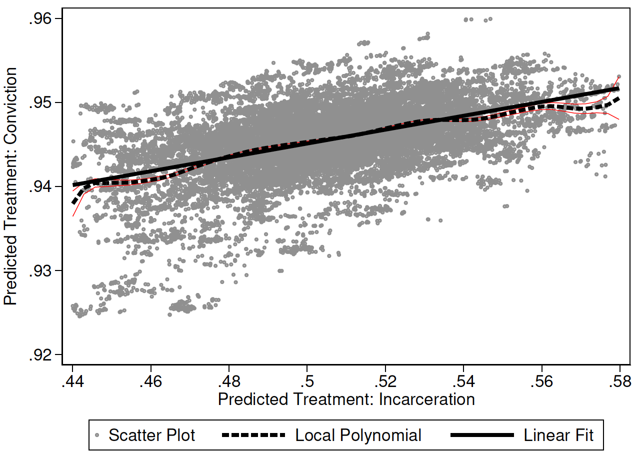
Figure B.2: Empirical Application: Testing Proposition 9.

Note: This figure shows a scatter plot of predicted conviction treatment ($P_{1}$) and predicted incarceration treatment ($P_{2}$) using data from Bhuller et al., (2020), along with a linear regression fit and local polynomial regression fit. The sample consists of 31,428 non-confession criminal cases that were quasi-randomly assigned to judges in Norwegian trial courts between 2005 and 2009. The local polynomial regression uses an Epanechnikov kernel with bandwidth of 0.01 and a third degree polynomial smoothing. The red lines show the 99 percent confidence intervals corresponding to the local polynomial regression. The linear regression of predicted conviction treatment ($P_{1}$) on predicted incarceration treatment ($P_{2}$) has a coefficient of 0.083 (SE=0.001), and the Ramsey’s RESET test of a linear functional form is rejected with an F-statistic of 445.1 (p-value=0.000). This provides a formal test of Proposition 9 under a single-index threshold-crossing model presented in Section 3.2. All estimations control for court by court entry year fixed effects and baseline controls listed in Bhuller et al., (2020), Table 1. Proposition B.6 shows that when the model includes court-by-year fixed effects, a linear relationship between $P_{1}$ and $P_{2}$ must exist within each court-by-year cell. For ease of illustration, we consider here the overall relationship.

Table B.2: Empirical Application: 2SLS with Multiple Treatments.

Outcome:	Recidivism $\left(Y\right)$
Specification:	Single Treatment	Multiple Treatments
	(1)	(2)
Treatments:
Conviction $\left(D_{1}\right)$	–	-0.222
		(0.819)
Incarceration $\left(D_{2}\right)$	-0.293***	-0.281**
	(0.106)	(0.126)
Dependent mean	0.70	0.70
Number of cases	31,428	31,428

Note: This table reports 2SLS estimates from model specification with a single binary treatment indicator for incarceration (Column 1) and multiple treatment indicators for conviction and incarceration (Column 2), respectively, and randomly assigned judges as instruments using data from Bhuller et al., (2020). The estimate reported in Column (1) is identical to the IV estimate reported in the final row of Table 4, Column (3), on p. 1297 in Bhuller et al., (2020). The sample consists of 31,428 non-confession criminal cases that were quasi-randomly assigned to judges in Norwegian trial courts between 2005 and 2009. All estimations control for court by court entry year fixed effects and baseline controls listed in Bhuller et al., (2020), Table 1. *p<0.1, **p<0.05, ***p<0.01.

Table B.3: Empirical Application: Testing Propositions 3 and 4.

A. Testing Proposition 3 for Ordered Treatments: $\left\{D_{1}=1\left[t\geq 1\right],D_{2}=1\left[t=2\right]\right\}$
	Recidivism $\left(Y\right)$				No Recidivism $\left(1-Y\right)$
Outcomes:	$Y\left(D_{1}-D_{2}\right)$	$YD_{2}$		Outcomes:	$\left(1-Y\right)\left(D_{1}-D_{2}\right)$		$\left(1-Y\right)D_{2}$
Regressors:	(1)	(2)		Regressors:	(3)		(4)
Predicted Conviction $(P_{1})$	1.173 (1.005)	-0.689 (1.267)		Predicted Conviction $(P_{1})$	-0.173 (0.844)		0.689 (0.659)
Predicted Incarceration $(P_{2})$	-0.780*** (0.169)	0.482** (0.199)		Predicted Incarceration $(P_{2})$	-0.220* (0.124)		0.518*** (0.129)
$H0:\vartheta_{11}\geq 0,\vartheta_{21}=0$	[0.878]	[0.587]		$H0:\psi_{11}\geq 0,\psi_{21}=0$	[0.419]		[0.297]
$H0:\vartheta_{22}\geq 0$	–	[0.992]		$H0:\psi_{22}\geq 0$	–		[1.000]
$H0:\vartheta_{22}+\vartheta_{12}=0$	[0.123]			$H0:\psi_{22}+\psi_{12}=0$	[0.080]
Observations:	31,428			Observations:	31,428
B. Testing Proposition 4 for Ordered Treatments: $\left\{D_{1}=1\left[t\geq 1\right],D_{2}=1\left[t=2\right]\right\}$
Outcomes:	Conviction $\left(D_{1}\right)$			Incarceration $\left(D_{2}\right)$
Regressors:	Predicted Conviction $(P_{1})$	Predicted Incarceration $(P_{2})$		Predicted Conviction $(P_{1})$	Predicted Incarceration $(P_{2})$		Observations:
Sub-samples:	(1)	(2)		(3)	(4)		(5)
Previously Employed	1.275** (0.523)	0.110 (0.085)		-0.127 (1.092)	1.195*** (0.178)		16,547
$H0:\eta_{11}\geq 0,\eta_{12}=\eta_{21}=0,\eta_{22}\geq 0$	[0.993]	[0.197]		[0.908]	[1.000]
Previously Non-Employed	0.641 (0.496)	-0.118 (0.079)		0.010 (1.162)	0.788*** (0.186)		14,881
$H0:\eta_{11}\geq 0,\eta_{12}=\eta_{21}=0,\eta_{22}\geq 0$	[0.902]	[0.137]		[0.920]	[1.000]
Previously Incarcerated	1.239*** (0.401)	0.062 (0.065)		-0.571 (1.084)	1.104*** (0.175)		16,042
$H0:\eta_{11}\geq 0,\eta_{12}=\eta_{21}=0,\eta_{22}\geq 0$	[0.999]	[0.339]		[0.598]	[1.000]
Previously Non-Incarcerated	0.883 (0.607)	-0.078 (0.098)		1.245 (1.116)	0.820*** (0.180)		15,386
$H0:\eta_{11}\geq 0,\eta_{12}=\eta_{21}=0,\eta_{22}\geq 0$	[0.927]	[0.424]		[0.265]	[1.000]
Young (Age < 30)	1.498*** (0.488)	-0.055 (0.079)		-1.049 (1.114)	1.131*** (0.182)		15,956
$H0:\eta_{11}\geq 0,\eta_{12}=\eta_{21}=0,\eta_{22}\geq 0$	[0.999]	[0.489]		[0.347]	[1.000]
Old (Age > 30)	0.483 (0.537)	0.055 (0.086)		1.088 (1.135)	0.870*** (0.181)		15,472
$H0:\eta_{11}\geq 0,\eta_{12}=\eta_{21}=0,\eta_{22}\geq 0$	[0.816]	[0.519]		[0.338]	[1.000]
Below High School	1.238*** (0.404)	-0.064 (0.065)		-0.766 (0.945)	1.025*** (0.152)		22,651
$H0:\eta_{11}\geq 0,\eta_{12}=\eta_{21}=0,\eta_{22}\geq 0$	[0.999]	[0.322]		[0.417]	[1.000]
High School or Above	0.403 (0.763)	0.169 (0.125)		1.855 (1.476)	0.949*** (0.242)		8,777
$H0:\eta_{11}\geq 0,\eta_{12}=\eta_{21}=0,\eta_{22}\geq 0$	[0.701]	[0.176]		[0.209]	[1.000]
Had Children	1.248** (0.631)	0.070 (0.100)		1.672 (1.331)	0.973*** (0.211)		11,717
$H0:\eta_{11}\geq 0,\eta_{12}=\eta_{21}=0,\eta_{22}\geq 0$	[0.976]	[0.484]		[0.209]	[1.000]
Had No Children	0.875** (0.440)	-0.042 (0.072)		-0.931 (0.993)	1.013*** (0.162)		19,711
$H0:\eta_{11}\geq 0,\eta_{12}=\eta_{21}=0,\eta_{22}\geq 0$	[0.977]	[0.563]		[0.349]	[1.000]
Low Incarceration Propensity	0.954* (0.548)	-0.040 (0.090)		-1.176 (1.101)	1.183*** (0.183)		15,714
$H0:\eta_{11}\geq 0,\eta_{12}=\eta_{21}=0,\eta_{22}\geq 0$	[0.959]	[0.657]		[0.285]	[1.000]
High Incarceration Propensity	1.058** (0.470)	0.038 (0.075)		1.233 (1.120)	0.805*** (0.179)		15,714
$H0:\eta_{11}\geq 0,\eta_{12}=\eta_{21}=0,\eta_{22}\geq 0$	[0.988]	[0.615]		[0.271]	[1.000]

Note: This table reports tests of Proposition 3 generalized to ordered treatments in Section B.2.1 (Panel A) and Proposition 4 (Panel B) using data from Bhuller et al., (2020). See Section 5.2 for the corresponding regression specifications. Proposition B.2 shows that Proposition 3 extends to the case with control variables, while Proposition B.3 provides a generalization of Proposition 4 under Assumption B.3. The sample consists of 31,428 non-confession criminal cases that were quasi-randomly assigned to judges in Norwegian trial courts between 2005 and 2009. All estimations control for court by court entry year fixed effects and baseline controls listed in Bhuller et al., (2020), Table 1. For each observation, we estimate an incarceration propensity using pre-determined case and defendant characteristics listed in Bhuller et al., (2020), Table 1, based on a logit model, and create subsamples by low and high propensity based on the median predicted propensity in the final two rows of Panel B. *p<0.1, **p<0.05, ***p<0.01.

References

- Acemoglu & Johnson, (2005) Acemoglu, Daron, & Johnson, Simon. 2005. Unbundling institutions. Journal of political Economy, 113(5), 949–995.
- Angrist et al., (2009) Angrist, Joshua, Lang, Daniel, & Oreopoulos, Philip. 2009. Incentives and services for college achievement: Evidence from a randomized trial. American Economic Journal: Applied Economics, 1(1), 136–63.
- Angrist et al., (2022) Angrist, Joshua, Hull, Peter, & Walters, Christopher R. 2022. Methods for Measuring School Effectiveness. NBER WP No. 30803.
- Angrist, (2006) Angrist, Joshua D. 2006. Instrumental variables methods in experimental criminological research: what, why and how. Journal of Experimental Criminology, 2, 23–44.
- Angrist & Imbens, (1995) Angrist, Joshua D., & Imbens, Guido W. 1995. Two-Stage Least Squares Estimation of Average Causal Effects in Models with Variable Treatment Intensity. Journal of the American Statistical Association, 90(430), 431–442.
- Autor et al., (2015) Autor, David, Maestas, Nicole, Mullen, Kathleen J, Strand, Alexander, et al. 2015. Does delay cause decay? The effect of administrative decision time on the labor force participation and earnings of disability applicants. NBER WP No. 20840.
- Behaghel et al., (2013) Behaghel, Luc, Crepon, Bruno, & Gurgand, Marc. 2013. Robustness of the Encouragement Design in a Two-Treatment Randomized Control Trial. IZA DP 7447.
- Bhuller et al., (2020) Bhuller, Manudeep, Dahl, Gordon B., Løken, Katrine V., & Mogstad, Magne. 2020. Incarceration, Recidivism, and Employment. Journal of Political Economy, 128(4), 1269–1324.
- Blandhol et al., (2022) Blandhol, Christine, Bonney, John, Mogstad, Magne, & Torgovitsky, Alexander. 2022. When is TSLS Actually LATE? NBER WP No. 29709.
- Bombardini & Li, (2020) Bombardini, Matilde, & Li, Bingjing. 2020. Trade, pollution and mortality in China. Journal of International Economics, 125, 103321.
- Borusyak et al., (2021) Borusyak, Kirill, Jaravel, Xavier, & Spiess, Jann. 2021. Revisiting event study designs: Robust and efficient estimation. arXiv preprint arXiv:2108.12419.
- Callaway & Sant’Anna, (2021) Callaway, Brantly, & Sant’Anna, Pedro HC. 2021. Difference-in-differences with multiple time periods. Journal of Econometrics, 225(2), 200–230.
- Carneiro et al., (2003) Carneiro, Pedro, Hansen, Karsten T, & Heckman, James J. 2003. Estimating distributions of treatment effects with an application to the returns to schooling and measurement of the effects of uncertainty on college choice. International Economic Review, 44(2), 361–422.
- Chernozhukov et al., (2013) Chernozhukov, Victor, Lee, Sokbae, & Rosen, Adam M. 2013. Intersection bounds: Estimation and inference. Econometrica, 81(2), 667–737.
- Cunha et al., (2007) Cunha, Flavio, Heckman, James J, & Navarro, Salvador. 2007. The identification and economic content of ordered choice models with stochastic thresholds. International Economic Review, 48(4), 1273–1309.
- de Chaisemartin & d’Haultfoeuille, (2020) de Chaisemartin, Clément, & d’Haultfoeuille, Xavier. 2020. Two-way fixed effects estimators with heterogeneous treatment effects. American Economic Review, 110(9), 2964–96.
- de Chaisemartin & d’Haultfoeuille, (2023) de Chaisemartin, Clément, & d’Haultfoeuille, Xavier. 2023. Two-way fixed effects regressions with several treatments. Journal of Econometrics, 236(2).
- Dobbie et al., (2018) Dobbie, Will, Goldin, Jacob, & Yang, Crystal S. 2018. The Effects of Pretrial Detention on Conviction, Future Crime, and Employment: Evidence from Randomly Assigned Judges. American Economic Review, 108(2), 201–40.
- Farbmacher et al., (2022) Farbmacher, Helmut, Guber, Raphael, & Klaassen, Sven. 2022. Instrument validity tests with causal forests. Journal of Business & Economic Statistics, 40(2), 605–614.
- Frandsen et al., (2023) Frandsen, Brigham, Lefgren, Lars, & Leslie, Emily. 2023. Judging Judge Fixed Effects. American Economic Review, 113(1), 253–77.
- Galindo, (2020) Galindo, Camila. 2020. Empirical Challenges of Multivalued Treatment Effects. Unpublished.
- Goff, (2020) Goff, Leonard. 2020. A Vector Monotonicity Assumption for Multiple Instruments. arXiv preprint arXiv:2009.00553.
- Goldsmith-Pinkham et al., (2022) Goldsmith-Pinkham, Paul, Hull, Peter, & Kolesár, Michal. 2022. Contamination bias in linear regressions. NBER WP No. 30108.
- Goodman-Bacon, (2021) Goodman-Bacon, Andrew. 2021. Difference-in-differences with variation in treatment timing. Journal of Econometrics, 225(2), 254–277.
- Greene & Hensher, (2010) Greene, William H, & Hensher, David A. 2010. Modeling ordered choices: A primer. Cambridge University Press.
- Heckman, (1979) Heckman, James J. 1979. Sample selection bias as a specification error. Econometrica, 47(1), 153–161.
- Heckman & Pinto, (2018) Heckman, James J, & Pinto, Rodrigo. 2018. Unordered monotonicity. Econometrica, 86(1), 1–35.
- Heckman & Vytlacil, (1999) Heckman, James J, & Vytlacil, Edward J. 1999. Local Instrumental Variables and Latent Variable Models for Identifying and Bounding Treatment Effects. Proceedings of the National Academy of Sciences, 96(8), 4730–4734.
- Heckman & Vytlacil, (2005) Heckman, James J, & Vytlacil, Edward J. 2005. Structural Equations, Treatment Effects, and Econometric Policy Evaluation. Econometrica, 73(3), 669–738.
- Heckman & Vytlacil, (2007) Heckman, James J, & Vytlacil, Edward J. 2007. Econometric evaluation of social programs, part II: Using the marginal treatment effect to organize alternative econometric estimators to evaluate social programs, and to forecast their effects in new environments. Handbook of Econometrics, 6, 4875–5143.
- Heckman et al., (2008) Heckman, James J., Urzua, Sergio, & Vytlacil, Edward. 2008. Instrumental Variables in Models with Multiple Outcomes: the General Unordered Case. Annales d’Economie et de Statistique, 151–174.
- Heinesen et al., (2022) Heinesen, Eskil, Hvid, Christian, Kirkebøen, Lars Johannessen, Leuven, Edwin, & Mogstad, Magne. 2022. Instrumental Variables with Unordered Treatments: Theory and Evidence from Returns to Fields of Study. NBER WP No. 30574.
- Humphries et al., (2023) Humphries, John Eric, Ouss, Aurélie, Stevenson, Megan, Stavreva, Kamelia, & van Dijk, Winnie. 2023. Conviction, Incarceration, and Recidivism: Understanding the Revolving Door. SSRN ID No. 4507597.
- Imbens & Angrist, (1994) Imbens, Guido W, & Angrist, Joshua D. 1994. Identification and Estimation of Local Average Treatment Effects. Econometrica, 62(2), 467–475.
- Jaeger et al., (2018) Jaeger, David A, Ruist, Joakim, & Stuhler, Jan. 2018. Shift-share instruments and the impact of immigration. NBER WP No. 24285.
- Kamat et al., (2023a) Kamat, Vishal, Norris, Samuel, & Pecenco, Matthew. 2023a. Conviction, Incarceration, and Policy Effects in the Criminal Justice System.
- Kamat et al., (2023b) Kamat, Vishal, Norris, Samuel, & Pecenco, Matthew. 2023b. Identification in Multiple Treatment Models under Discrete Variation. arXiv preprint arXiv:2307.06174.
- Kirkeboen et al., (2016) Kirkeboen, Lars J., Leuven, Edwin, & Mogstad, Magne. 2016. Field of Study, Earnings, and Self-Selection. Quarterly Journal of Economics, 131(3), 1057–1111.
- Kitagawa, (2015) Kitagawa, Toru. 2015. A test for instrument validity. Econometrica, 83(5), 2043–2063.
- Kline & Walters, (2016) Kline, Patrick, & Walters, Christopher R. 2016. Evaluating public programs with close substitutes: The case of Head Start. Quarterly Journal of Economics, 131(4), 1795–1848.
- Lee & Salanié, (2018) Lee, Sokbae, & Salanié, Bernard. 2018. Identifying effects of multivalued treatments. Econometrica, 86(6), 1939–1963.
- Lee & Salanié, (2023) Lee, Sokbae, & Salanié, Bernard. 2023. Filtered and Unfiltered Treatment Effects with Targeting Instruments. arXiv preprint arXiv:2007.10432.
- Mogstad et al., (2021) Mogstad, Magne, Torgovitsky, Alexander, & Walters, Christopher R. 2021. The Causal Interpretation of Two-Stage Least Squares with Multiple Instrumental Variables. American Economic Review, 3663–3698.
- Mogstad et al., (forthcoming) Mogstad, Magne, Torgovitsky, Alexander, & Walters, Christopher R. forthcoming. Policy evaluation with multiple instrumental variables. Journal of Econometrics.
- Mountjoy, (2022) Mountjoy, Jack. 2022. Community colleges and upward mobility. American Economic Review, 112(8), 2580–2630.
- Mourifié & Wan, (2017) Mourifié, Ismael, & Wan, Yuanyuan. 2017. Testing local average treatment effect assumptions. Review of Economics and Statistics, 99(2), 305–313.
- Mueller-Smith, (2015) Mueller-Smith, Michael. 2015. The Criminal and Labor Market Impacts of Incarceration. Working Paper.
- Norris et al., (2021) Norris, Samuel, Pecenco, Matthew, & Weaver, Jeffrey. 2021. The effects of parental and sibling incarceration: Evidence from ohio. American Economic Review, 111(9), 2926–63.
- Persson & Tabellini, (2004) Persson, Torsten, & Tabellini, Guido. 2004. Constitutional rules and fiscal policy outcomes. American Economic Review, 94(1), 25–45.
- Pinto, (2021) Pinto, Rodrigo. 2021. Beyond intention to treat: Using the incentives in moving to opportunity to identify neighborhood effects. Working Paper.
- Rohlfs, (2006) Rohlfs, Chris. 2006. The government’s valuation of military life-saving in war: A cost minimization approach. American Economic Review, 96(2), 39–44.
- Rose & Shem-Tov, (2021a) Rose, Evan K, & Shem-Tov, Yotam. 2021a. How does incarceration affect reoffending? estimating the dose-response function. Journal of Political Economy, 129(12), 3302–3356.
- Rose & Shem-Tov, (2021b) Rose, Evan K, & Shem-Tov, Yotam. 2021b. On Recoding Ordered Treatments as Binary Indicators. arXiv preprint arXiv:2111.12258.
- Słoczyński, (2020) Słoczyński, Tymon. 2020. When should we (not) interpret linear IV estimands as LATE? arXiv preprint arXiv:2011.06695.
- Sun & Abraham, (2021) Sun, Liyang, & Abraham, Sarah. 2021. Estimating dynamic treatment effects in event studies with heterogeneous treatment effects. Journal of Econometrics, 225(2), 175–199.
- Sun, (2023) Sun, Zhenting. 2023. Instrument validity for heterogeneous causal effects. Journal of Econometrics, 237(2).
- Vytlacil, (2002) Vytlacil, Edward. 2002. Independence, monotonicity, and latent index models: An equivalence result. Econometrica, 70(1), 331–341.