Decision Making for Hierarchical Multi-label Classification with Multidimensional Local Precision Rate

Abstract

Hierarchical multi-label classification (HMC) has drawn increasing attention in the past few decades. It is applicable when hierarchical relationships among classes are available and need to be incorporated along with the multi-label classification whereby each object is assigned to one or more classes. There are two key challenges in HMC: i) optimizing the classification accuracy, and meanwhile ii) ensuring the given class hierarchy. To address these challenges, in this article, we introduce a new statistic called the multidimensional local precision rate (mLPR) for each object in each class. We show that classification decisions made by simply sorting objects across classes in descending order of their true mLPRs can, in theory, ensure the class hierarchy and lead to the maximization of CATCH, an objective function we introduce that is related to the area under a hit curve. This approach is the first of its kind that handles both challenges in one objective function without additional constraints, thanks to the desirable statistical properties of CATCH and mLPR. In practice, however, true mLPRs are not available. In response, we introduce HierRank, a new algorithm that maximizes an empirical version of CATCH using estimated mLPRs while respecting the hierarchy. The performance of this approach was evaluated on a synthetic data set and two real data sets; ours was found to be superior to several comparison methods on evaluation criteria based on metrics such as precision, recall, and $F_{1}$ score.

Keywords hierarchical multi-label classification, HierRank, hit curve, mLPR, multidimensional local precision rate

1 Introduction

Hierarchical multi-label classification (HMC) refers to the task involved when additional knowledge of the dependency relationships among classes is available and needs to be incorporated along with the multi-label classification by which each object is assigned to one or more classes (Zhang and Zhou, 2013). The class dependency in HMC is usually assumed to follow a hierarchical structure represented by a tree or a directed acyclic graph (DAG). HMC, an important problem in many applications, has recently attracted much attention in statistics and machine learning research. In biology and biomedicine, HMC applications include the diagnosis of disease along a DAG composed of terms from the Unified Medical Language System (UMLS) (Huang et al., 2010; Jiang et al., 2014), the assignment of genes to multiple gene functional categories defined by the Gene Ontology DAG (Alves et al., 2010; Feng et al., 2017; Kahanda and Ben-Hur, 2017), the categorization of MIPS FunCat rooted tree (Valentini, 2011), and numerous other biomedical examples (Chen et al., 2019; Makrodimitris et al., 2019; Nakano et al., 2019; Pham et al., 2021). Outside of biology, HMC is commonly used in text classification, music categorization, and image recognition (Gupta et al., 2016; Salama and El-Gohary, 2016; Zeng et al., 2017; Yang et al., 2018).

A seminal line of HMC research has addressed the problem via a two-stage approach. In the first stage, classifiers are trained for each class with no consideration of the class hierarchy, as if there were multiple independent classification problems. The task of the second stage is then to render a decision regarding each class for each object based on the class hierarchy and a predefined performance criterion, given the classifier scores from the first stage (Silla and Freitas, 2011; Feng et al., 2017; Chen et al., 2019). This approach is popular for its flexibility (as a variety of classification methods can be applied in the first stage) as well as its computational efficiency (as the class-specific classifiers can be trained in parallel). However, it remains an open question at the second stage how to balance the two key challenges in HMC: 1) respecting the given class hierarchy and 2) achieving the best possible classification performance as evaluated by metrics such as accuracy, precision, recall, and F-measure.

Within this two-stage approach, some methods make decisions based on class-specific cutoffs for the first-stage classifier scores, determining the cutoff values by optimizing an objective such as H-loss or F-measure (Barutcuoglu et al., 2006; Triguero and Vens, 2016). As the cutoff values are determined without full consideration of the hierarchical structure (they may even be determined independently of each other), the class decisions may not respect the hierarchy. Although such decisions can be adjusted to satisfy the hierarchical constraint through a remedying procedure, this brings with it a problem of its own: the remedied decisions may no longer be optimal with respect to the original performance objective (Ananpiriyakul et al., 2014).

Other methods proceed with the second stage by ranking the objects across all classes, given the class hierarchy and the classifier scores of the objects in every class. In this treatment, a single cutoff on the ranking suffices to produce all of the decisions. Jiang et al. (2014) described a way to optimally rank all of the objects across all classes in the general multi-label problem: transforming the first-stage classifier scores to local precision rates (LPRs) and then obtaining a ranking by sorting the LPRs in descending order. It was shown that the resulting ranking maximizes the pooled precision rate at any pooled recall rate. The LPR concept is also attractive in that it lends itself to a Bayesian interpretation; its value is equivalent to the local true discovery rate ($\ell$tdr) under certain probabilistic assumptions. However, this method does not consider the hierarchical structure. Bi and Kwok (2011) used an algorithm that maximizes the sum of the top $L$ first-stage classifier scores while respecting the hierarchy, where $L$ is predefined. This method can produce a ranking of all of objects across classes by varying $L$. Nonetheless, it might be inappropriate to sum these classifier scores directly because of potential statistical differences among the classifiers for different classes. If this is not properly handled, such differences can lead to poor decisions; see Appendix D.5 for an illustration. Bi and Kwok (2015) extended Bi and Kwok (2011) by introducing an algorithm to optimize some objective function (instead of the sum of the top $L$ classifier scores) under the hierarchical constraint. Although they investigated three candidate objective/risk functions, they did not suggest which of these to use. Moreover, they did not provide a clear statistical interpretation or justification of the three risk functions nor of their hyperparameters.

In this article, we introduce a new statistic, called the multidimensional local precision rate (mLPR), for each object in each class, which can be derived based on the first-stage classifier scores and the hierarchy. Like LPR, mLPR lends itself to a Bayesian interpretation: under certain probabilistic assumptions, it is equivalent to the multidimensional local true discovery rate (m$\ell$tdr) used in hierarchical hypothesis testing (Ploner et al., 2006). We show that sorting objects across classes in descending order by their mLPRs ensures hierarchical consistency and maximizes a new objective function, called the conditional expected area under the curve of hit and denoted by “CATCH.” This objective is designed based on the hit curve (Herskovic et al., 2007), which is chosen for practicality; see Section 3.1 for a detailed discussion. To the best of our knowledge, this approach is the first of its kind that handles the two aforementioned HMC challenges in one objective without the need of extra constraints.

In practice, we will need to estimate mLPRs from data. However, sorting the estimated mLPRs in descending order might fail to guarantee the optimization of CATCH or may violate the hierarchy consistency. To address this issue, we develop an algorithm for Hierarchical Ranking, called HierRank, that maximizes an empirical version of CATCH based on the estimated mLPRs while respecting the hierarchical constraint. In addition, we propose a cutoff selection procedure that makes decisions on the resulting ranking according to a given purpose, e.g., controlling the false discovery rate (FDR) at a given significance level or achieving the maximum $F_{1}$ score.

We compared our method to several state-of-the-art HMC methods using a synthetic data set and two real data sets; ours outperformed comparison methods on evaluation metrics such as precision, recall and $F_{1}$ score. We also investigated how the accuracy of the mLPR estimation influences the method’s performance.

The rest of the paper is organized as follows. In Section 2, we introduce our model. In Section 3, we introduce the objective function CATCH and the statistic mLPR, and we show that sorting mLPRs in descending order can maximize CATCH while respecting the hierarchy. In Section 4, we propose the ranking algorithm HierRank, which sorts objects by estimated mLPRs under the hierarchy constraint. The performance of the method on a synthetic data set and present two case studies is reported in Section 5. Finally, we conclude the article in Section 6. The supplementary information can be found in the appendices.

2 Notation and Model

2.1 Notation

Suppose there are $K$ classes that are structured in a hierarchy $\operatorname*{\mathcal{G}}$, as, for example, in Figure 1 (a). In $\operatorname*{\mathcal{G}}$, denote by $pa(k)$ the set of the parent nodes of the $k$th node, by $anc(k)$ the set of its ancestor nodes, and by $nbh(k)$ the set of its immediate neighbors. In the example shown in the figure, for instance, $pa(\text{F})=\{\text{C}\}$, $anc(\text{F})=\{\text{A},\text{C}\}$, and $nbh(\text{F})=\{\text{C},\text{G},\text{I}\}$.

A given random object (an item to be classified) may have multiple positive labels from the $K$ classes, corresponding to $K$ classification decisions to be made. Throughout this article, when a classifier assigns a positive membership to an object for a given class, we call it a “classification event” (or “event” when no confusion arises). Each event is associated with a binary variable $Y$, which indicates the corresponding true class status of the object under consideration, and a pre-given classifier score $S$, which reflects the likelihood of the event occurring. Specifically, for a given random object, $Y_{k}$ and $S_{k}$ denote the true status and the classifier score, respectively, for the $k$th class. $\operatorname*{\boldsymbol{Y}}$ denotes $(Y_{1},\ldots,Y_{K})^{\operatorname*{\text{T}}}$, and $\operatorname*{\boldsymbol{S}}$ denotes $(S_{1},\ldots,S_{K})^{\operatorname*{\text{T}}}$. $\operatorname*{\boldsymbol{Y}}_{D}$ denotes $(Y_{k})^{\operatorname*{\text{T}}}_{k\in D}$, and $\operatorname*{\boldsymbol{S}}_{D}$ denotes $(S_{k})^{\operatorname*{\text{T}}}_{k\in D}$ for a subset $D\subset\{1,\ldots,K\}$.

In practice, we observe $M$ objects, and there are $n=K\times M$ classification events in total. We use $Y_{k}^{(m)}$ and $S_{k}^{(m)}$ to denote the true status and the predefined classifier score, respectively, of the $k$th class for the $m$th object. For the $m$th object, $\operatorname*{\boldsymbol{Y}}^{(m)}$ denotes $(Y_{1}^{(m)},\ldots,Y_{K}^{(m)})^{\operatorname*{\text{T}}}$, and $\operatorname*{\boldsymbol{S}}^{(m)}$ denotes $(S_{1}^{(m)},\ldots,S_{K}^{(m)})^{\operatorname*{\text{T}}}$. For ease of notation, throughout the rest of the paper, we say that Event $i$ is an ancestor of Event $i^{\prime}$ (or, equivalently, $i\in anc(i^{\prime})$) if the two events $i$ and $i^{\prime}$ concern the same object and the class node associated with Event $i$ is an ancestor node of that of Event $i^{\prime}$. We define the ranking $\operatorname*{\boldsymbol{\pi}}=(\pi_{1},\ldots,\pi_{n})$ on $n$ events as a permutation of $(1,2,\ldots,n-1,n)$. We say a ranking $\operatorname*{\boldsymbol{\pi}}$ has hierarchical consistency or is a topological ordering for $\operatorname*{\mathcal{G}}$ if it satisfies

$$\pi_{i}<\pi_{i^{\prime}}\text{~{} for any Event $i$ that is an ancestor of Event $i^{\prime}$.}$$

2.2 Model

The hierarchy $\operatorname*{\mathcal{G}}$ for the $K$ classes is assumed to be a tree or a DAG. It can be disconnected and consist of multiple connected components, as in the example shown in Figure 1 (a). In this article, we focus mainly on the tree structure; the extension to the DAG structure is discussed in Appendix B.4.

We propose a model $\operatorname*{\mathcal{H}}$ to characterize the relationship between $\operatorname*{\boldsymbol{Y}}$ and $\operatorname*{\boldsymbol{S}}$ of a given random object. We make the following assumptions for the model:

• The scores are conditionally independent given the associated class labels; i.e.,

  $$S_{k^{\prime}}\perp S_{k}|Y_{k}\text{~{}~{}and~{}~{}}Y_{k^{\prime}}\perp S_{k}|Y_{k}\text{~{}~{}for any~{}~{}}k^{\prime}\neq k,$$

  which implies that $\operatorname*{\mathbb{P}}(S_{k}=s|S_{1},\ldots,S_{k-1},S_{k+1},\ldots,S_{K},Y_{1},\ldots,Y_{K})=\operatorname*{\mathbb{P}}(S_{k}=s|Y_{k})$.

• $\operatorname*{\mathbb{P}}(Y_{k}=1|\operatorname*{\boldsymbol{Y}}_{pa(k)}=\boldsymbol{1})\in[0,1]$; $\operatorname*{\mathbb{P}}(Y_{k}=1|\operatorname*{\boldsymbol{Y}}_{pa(k)}=\boldsymbol{0})=0$.

• $S_{k}$ has a mixture model; i.e., $\operatorname*{\mathbb{P}}(S_{k}\leq s)=\operatorname*{\mathbb{P}}(S_{k}\leq s,Y_{k}=0)+\operatorname*{\mathbb{P}}(S_{k}\leq s,Y_{k}=1)=F_{0,k}(s)\operatorname*{\mathbb{P}}(Y_{k}=0)+F_{1,k}(s)\operatorname*{\mathbb{P}}(Y_{k}=1)$, where $F_{0,k}$ denotes the null cumulative distribution function (CDF) $\operatorname*{\mathbb{P}}(S_{k}\leq s|Y_{k}=0)$, and $F_{1,k}$ denotes the alternative CDF $\operatorname*{\mathbb{P}}(S_{k}\leq s|Y_{k}=1)$, for the $k$th class.

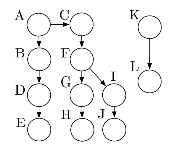
(a) An example hierarchy $\operatorname*{\mathcal{G}}$

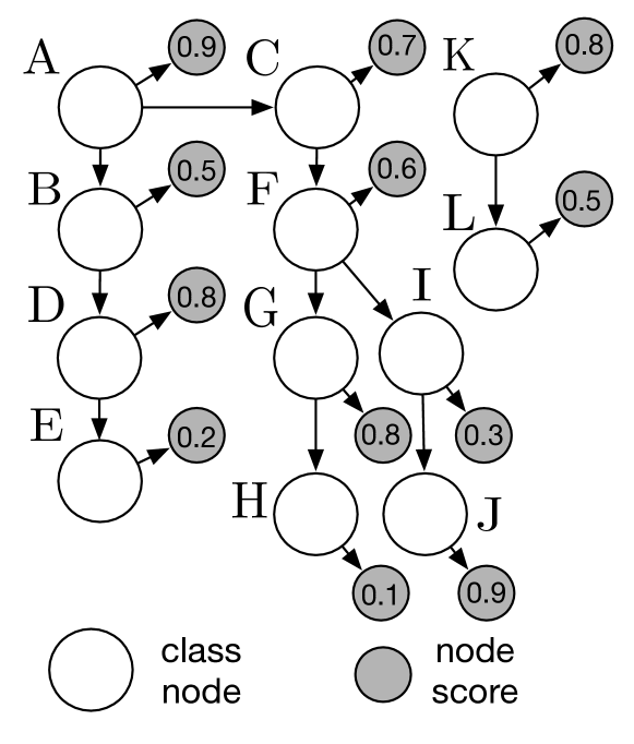
(b) The augmented graph $\operatorname*{\overline{\mathcal{G}}}$

Figure 1: Example hierarchical graph $\operatorname*{\mathcal{G}}$ and its associated augmented graph $\operatorname*{\overline{\mathcal{G}}}$.

Assumption (i) is reasonable for the two-stage method of HMC because the first-stage classification training is executed class by class. Based on the conditional independence, we consider an augmented graph $\operatorname*{\overline{\mathcal{G}}}$ (Figure 1 (b)) of $\operatorname*{\mathcal{G}}$. Assumption (ii) embodies the hierarchical consistency. Assumption (iii) introduces a two-mixture model for $S_{k}$ as $Y_{k}$ is binary.

We consider $M$ objects with $(\operatorname*{\boldsymbol{Y}}^{(m)},\operatorname*{\boldsymbol{S}}^{(m)})\overset{i.i.d.}{\sim}\operatorname*{\mathcal{H}}$, $m=1,\ldots,M$ (“i.i.d.” stands for “independent and identically distributed”). For a fixed class $k$, scores $\operatorname*{\boldsymbol{S}}^{(m)}:=\{S_{k}^{(m)}:m=1,\ldots,M\}$ follow the same mixture distribution. If $k$ and $k^{\prime}$ correspond to different nodes in $\operatorname*{\mathcal{G}}$, $S_{k}^{(m)}$ and $S_{k^{\prime}}^{(m^{\prime})}$ may follow different distributions and hence are not directly comparable (see Appendix D.5 for a detailed discussion). Therefore, when joint decisions are made across all nodes, such distinct statistical distributions across classes need to be taken into consideration.

3 The Multidimensional Local Precision Rate (mLPR)

In this section, we first introduce the objective function CATCH, whose definition is based on the hit curve. Optimizing CATCH leads to the proposed statistic, mLPR. We conclude the section by showing that mLPR has some attractive statistical properties and in particular that sorting mLPRs in descending order not only provides the optimal classification performance in terms of CATCH but guarantees hierarchical consistency as well.

For simplicity, we vectorize $(\operatorname*{\boldsymbol{Y}}^{(1)},\ldots,\operatorname*{\boldsymbol{Y}}^{(M)})$ and $(\operatorname*{\boldsymbol{S}}^{(1)},\ldots,\operatorname*{\boldsymbol{S}}^{(M)})$ to obtain $\operatorname*{\boldsymbol{\tilde{Y}}}=(Y_{1}^{(1)},\ldots,$ $Y_{K}^{(1)},\ldots,Y_{1}^{(M)},\ldots,Y_{K}^{(M)})^{\operatorname*{\text{T}}}$ and $\operatorname*{\boldsymbol{\tilde{S}}}=(S_{1}^{(1)},\ldots,S_{K}^{(1)},\ldots,S_{1}^{(M)},\ldots,S_{K}^{(M)})^{\operatorname*{\text{T}}}$, respectively. Letting $i=(m-1)\cdot K+k$, where $m$ denotes the object index and $k$ the class index, we rewrite $\operatorname*{\boldsymbol{\tilde{Y}}}=(Y_{1},\ldots,Y_{n})^{\operatorname*{\text{T}}}$, $\operatorname*{\boldsymbol{\tilde{S}}}=(S_{1},\ldots,S_{n})^{\operatorname*{\text{T}}}$ when there is no confusion. $\operatorname*{\boldsymbol{\tilde{Y}}}_{\tilde{D}}$ denotes $(Y_{i})^{\operatorname*{\text{T}}}_{i\in\tilde{D}}$, and $\operatorname*{\boldsymbol{\tilde{S}}}_{\tilde{D}}$ denotes $(S_{i})^{\operatorname*{\text{T}}}_{i\in\tilde{D}}$ for a subset $\tilde{D}\subset\{1,\ldots,n\}$. We use this notation throughout the rest of the paper.

3.1 Conditional Expected Area Under The Curve of Hit and Multidimensional Local Precision Rate

Given all $n$ classifier scores $\operatorname*{\boldsymbol{\tilde{S}}}$, we attempt to produce a reasonable ranking of the associated $n$ events based on the model $\operatorname*{\mathcal{H}}$ (described in Section 2.2). The natural question that arises is the choice of objective function that should be used to guide this ranking.

Here, we introduce the hit curve and the corresponding area under the curve (AUC), for which the x-axis represents the number of discoveries and the y-axis represents the number of true discoveries (i.e., the number of hits). There is a close connection between the hit curve and the precision–recall (PR) curve: the slope of the hit curve is the precision. Additionally, a large area under the hit curve corresponds to a large area under the PR curve. We prefer the hit curve because of two reasons: 1) it can serve well as a graphic representation of the ranker’s performance: it would plot the results along the x-axis in order of a given ranking, and the y-axis would indicate the results’ relevance to the true labels; 2) early decisions (corresponding to small numbers on the x-axis) lay more influence on the AUC of the hit curve than those made later (corresponding to large numbers on the x-axis). By contrast, the other traditional metrics, such as PR and receiver operating characteristic (ROC) curves, are not sensitive or informative to the top-ranked instances, especially when the number of true positive instances is tiny relative to the total number of determinations (Davis and Goadrich, 2006; Herskovic et al., 2007; Hand, 2009). Figure S1 in Appendix A provides an example of a hit curve.

Among all of the potential rankings that respect the class hierarchy, we wish to find the one that maximizes the area under the hit curve. Note the area under the hit curve when $x\in[i-1,i]$ is the number of true positives contained in the top $i$ predicted positives. Therefore, the total area under the hit curve can be expressed as

$$\text{area under hit curve}=\sum_{i=1}^{n}\sum_{j=1}^{i}\operatorname*{\mathbb{I}}(Y_{\pi_{j}}=1)=\sum_{i=1}^{n}(n-i+1)\operatorname*{\mathbb{I}}(Y_{\pi_{i}}=1),$$ (3.1)

where $\boldsymbol{\pi}$ refers to a ranking of all of the considered events, as defined in Section 2.1. As $Y_{\pi_{i}}$ is a random variable when the inputs are random objects, we consider the population mean of the area under the hit curve. Specifically, given the classifier scores $\operatorname*{\boldsymbol{\tilde{S}}}$, we take the conditional expected values of (3.1) to take into account the dependencies between classes, and we obtain

$$\text{CATCH\/}:=\operatorname*{\mathbb{E}}(\text{area~{}under~{}hit~{}curve}|\operatorname*{\boldsymbol{\tilde{S}}})=\sum_{i=1}^{n}(n-i+1)\operatorname*{\mathbb{P}}(Y_{\pi_{i}}=1|S_{1},\ldots,S_{n}).$$ (3.2)

This is our proposed objective function, the Conditional expected Area under The Curve of Hit (CATCH). We call $\operatorname*{\mathbb{P}}(Y_{1}=1|S_{1},\ldots,S_{n})$ the multidimensional local precision rate (mLPR); see Section 4.1 for a detailed discussion of its relationship to the statistic LPR (Jiang et al., 2014).

3.2 Properties of mLPR

The mLPR statistic is defined conditional on all of the scores $\operatorname*{\boldsymbol{\tilde{S}}}$, with a consideration of the dependencies between the scores. Proposition 1, given below, provides that the mLPR value of an event cannot be less than those of its descendants.

Proposition 1

Under Model $\operatorname*{\mathcal{H}}$ (defined in Section 2.2), for two events $i$ and $i^{\prime}$, if $i\in anc(i^{\prime})$, then $mLPR_{i}\geq mLPR_{i^{\prime}}$. By the definition of $anc(i^{\prime})$ (Section 2.1), the two events $i$ and $i^{\prime}$ concern the same object and the associated class node of Event $i$ is an ancestor of that of Event $i^{\prime}$.

Proof  For any $i^{\prime}$ and $i\in anc(i^{\prime})$, it follows that

$$mLPR_{i^{\prime}} = \operatorname*{\mathbb{P}}(Y_{i^{\prime}}=1|S_{1},\cdots,S_{n})$$

$$= \sum_{Y_{1},\cdots,Y_{i^{\prime}-1},Y_{i^{\prime}+1},\cdots,Y_{n}}\operatorname*{\mathbb{P}}(Y_{1},\cdots,Y_{i^{\prime}-1},Y_{i^{\prime}}=1,Y_{i^{\prime}+1},\cdots,Y_{n}|S_{1},\cdots,S_{n})$$

$$\overset{(a)}{=} \sum_{Y_{j}:{j\neq i,j\neq i^{\prime}}}\operatorname*{\mathbb{P}}(Y_{1},\cdots,Y_{i^{\prime}}=1,Y_{i}=1,\cdots,Y_{n}|S_{1},\cdots,S_{n})$$

$$\leq \sum_{{Y_{j}}:{j\neq i}}\operatorname*{\mathbb{P}}(Y_{1},\cdots,Y_{i-1},Y_{i}=1,Y_{i+1},\cdots,Y_{n}|S_{1},\cdots,S_{n})$$

$$= mLPR_{i},$$

where $(a)$ is obtained by Assumption (ii) for the model $\operatorname*{\mathcal{H}}$ (Section 2.2).  

Proposition 2 further provides that regardless of the dependencies, an event with a higher mLPR is more likely to occur than an event with a lower mLPR.

Proposition 2

Given Model $\operatorname*{\mathcal{H}}$ as defined in Section 2.2, for any events $i$ and $i^{\prime}$ for which $mLPR_{i}\geq mLPR_{i^{\prime}}$, we have

$$\operatorname*{\mathbb{P}}(Y_{i}=1|mLPR_{i}\geq mLPR_{i^{\prime}})\geq\operatorname*{\mathbb{P}}(Y_{i^{\prime}}=1|mLPR_{i}\geq mLPR_{i^{\prime}}).$$

Proof  For a realization $\operatorname*{\boldsymbol{\tilde{s}}}$ of $\operatorname*{\boldsymbol{\tilde{S}}}$, we have $\operatorname*{\mathbb{P}}(Y_{i}=1|\operatorname*{\boldsymbol{\tilde{S}}}=\operatorname*{\boldsymbol{\tilde{s}}})=mLPR_{i}\geq mLPR_{i^{\prime}}=\operatorname*{\mathbb{P}}(Y_{i^{\prime}}=1|\operatorname*{\boldsymbol{\tilde{S}}}=\operatorname*{\boldsymbol{\tilde{s}}})$. The desired result follows by

$$\operatorname*{\mathbb{P}}(Y_{i}=1,mLPR_{i}\geq mLPR_{i^{\prime}})$$

$$= \int_{\operatorname*{\boldsymbol{\tilde{s}}}:mLPR_{i}\geq mLPR_{i^{\prime}}}\operatorname*{\mathbb{P}}(Y_{i}=1,\operatorname*{\boldsymbol{\tilde{S}}}=\operatorname*{\boldsymbol{\tilde{s}}})d{\operatorname*{\boldsymbol{\tilde{s}}}}$$

$$\geq \int_{\operatorname*{\boldsymbol{\tilde{s}}}:mLPR_{i}\geq mLPR_{i^{\prime}}}\operatorname*{\mathbb{P}}(Y_{i^{\prime}}=1,\operatorname*{\boldsymbol{\tilde{S}}}=\operatorname*{\boldsymbol{\tilde{s}}})d{\operatorname*{\boldsymbol{\tilde{s}}}}=\operatorname*{\mathbb{P}}(Y_{i^{\prime}}=1,mLPR_{i}\geq mLPR_{i^{\prime}}).$$

 

Proposition 1 implies that mLPRs can ensure hierarchical consistency, and Proposition 2 indicates that events from different classes can be compared using mLPRs. Taken together, these two propositions provide a statistical justification for directly comparing mLPRs in a scenario in which there exist dependencies between classes.

3.3 Sorting mLPRs in Descending Order

Recall (from Section 2.1) that a ranking $\boldsymbol{\pi}$ is hierarchically consistent if $\pi_{i}<\pi_{i^{\prime}}$ when Event $i$ is an ancestor of Event $i^{\prime}$. We wish to find the ranking that maximizes CATCH (3.2) while respecting the hierarchy. This can be expressed as the following optimization problem.

$$\max_{\operatorname*{\boldsymbol{\pi}}} CATCH\/$$ (3.3)

s.t. $$\text{$\boldsymbol{\pi}$ is hierarchically consistent}.$$

A ranking can be generated by naively sorting any scores (here, we use mLPRs) from highest to lowest. We call this type of ranking NaiveSort. Proposition 1 indicates that the ranking obtained by applying NaiveSort to mLPRs satisfies hierarchical consistency, and Proposition 2 implies that this ranking maximizes CATCH. Stated more specifically, by the definition of CATCH (3.2), its maximum is obtained by sorting mLPRs in descending order. In short, applying NaiveSort to the population of mLPRs solves the constrained optimization problem (3.3).

4 Ranking Algorithm Based on Estimated mLPRs

In this section, we describe how mLPRs are estimated using given observed classifier scores and a hierarchy. Then, we develop a ranking method for maximizing the empirical value of CATCH using the estimated mLPRs while respecting the hierarchy. Finally, we summarize the procedure for the method as a whole and provide a cutoff selection approach for making decisions based on the resulting ranking.

4.1 Computation of mLPRs

In most real-world scenarios, true mLPRs are not observable. We present a procedure for estimating mLPRs using the classifier scores $\operatorname*{\boldsymbol{\tilde{S}}}$, the true labels $\operatorname*{\boldsymbol{\tilde{Y}}}$, and the model $\operatorname*{\mathcal{H}}$. Note that $mLPR_{i}:=\operatorname*{\mathbb{P}}(Y_{i}|S_{1},\cdots,S_{n})=\sum_{Y_{1},\cdots,Y_{i-1},Y_{i+1},\cdots,Y_{n}}\operatorname*{\mathbb{P}}(Y_{1},\cdots,Y_{n}|S_{1},\cdots,S_{n})$. We compute $\operatorname*{\mathbb{P}}(Y_{1},\cdots,Y_{n}|S_{1},\cdots,S_{n})$ in a simple manner:

$$\operatorname*{\mathbb{P}}(Y_{1},\cdots,Y_{n}|S_{1},\cdots,S_{n}) \overset{(a)}{\propto} \operatorname*{\mathbb{P}}(S_{1},\cdots,S_{n}|Y_{1},\cdots,Y_{n})\cdot\operatorname*{\mathbb{P}}(Y_{1},\cdots,Y_{n})$$ (4.1)

$$\overset{(b)}{=} \prod_{i=1}^{n}\operatorname*{\mathbb{P}}(S_{i}|Y_{i})\operatorname*{\mathbb{P}}(Y_{i}|\boldsymbol{\tilde{Y}}_{pa(i)})$$

$$\overset{(c)}{\propto} \prod_{i=1}^{n}\frac{\operatorname*{\mathbb{P}}(Y_{i}|S_{i})}{\operatorname*{\mathbb{P}}(Y_{i})}\cdot\operatorname*{\mathbb{P}}(Y_{i}|\boldsymbol{\tilde{Y}}_{pa(i)})$$

$$\overset{(d)}{=} \prod_{i=1}^{n}LPR_{i}\cdot\frac{\operatorname*{\mathbb{P}}(Y_{i}|\boldsymbol{\tilde{Y}}_{pa(i)})}{\operatorname*{\mathbb{P}}(Y_{i})},$$

where $(a)$ and $(c)$ hold by Bayes’ rule, $(b)$ holds by using the Markov property with Assumption (i) for the model $\operatorname*{\mathcal{H}}$ (conditional independence), and $(d)$ follows from Jiang et al. (2014) that given the scores $\operatorname*{\boldsymbol{\tilde{S}}}$, the associated LPR for the $i$th node is defined as

$$LPR_{i}=\operatorname*{\mathbb{P}}(Y_{i}|S_{i}).$$

The LPR value is equivalent to the local true discovery rate ($\ell$tdr) under a Bayesian framework with certain probabilistic assumptions (Jiang et al., 2014). Similarly, mLPR is equivalent to m$\ell$tdr under the same Bayesian framework (Ploner et al., 2006). Therefore, mLPR is a multidimensional extension of LPR even though their derivations differ. Moreover, Jiang et al. (2014) proves that in the absence of a hierarchy, sorting events in descending order by their associated LPRs maximizes the pooled precision rate at any pooled recall rate. This result can also be extended to mLPRs in the HMC scenario.

We estimate LPRs by applying the method provided in Jiang et al. (2014) and estimate $\operatorname*{\mathbb{P}}(Y_{i}|\operatorname*{\boldsymbol{\tilde{Y}}}_{pa(i)})$ and $\operatorname*{\mathbb{P}}(Y_{i})$ using the empirical proportions (i.e., counting the number of objects with $Y_{k}=1$ to estimate $\operatorname*{\mathbb{P}}(Y_{k})$). Then, we use these estimates to obtain an estimator $\widehat{mLPR}$ of mLPR by applying sum–product message-passing to (4.1) with respect to $\operatorname*{\mathcal{G}}$ (Wainwright and Jordan, 2008).

Theorem 3

Under Assumptions A1, A2, and A3 given in Appendix E.1, by employing the kernel density estimator to estimate $LPR$ values (estimating the densities of $F_{0,k}$ and $F_{1,k}$ and thereby obtaining $LPR$) and employing the empirical estimators to estimate $\operatorname*{\mathbb{P}}(Y_{i})$ values and $\operatorname*{\mathbb{P}}(Y_{i}|\operatorname*{\boldsymbol{\tilde{Y}}}_{pa(i)})$ values, it follows that with probability at least $1-C_{1}\cdot K\cdot 2^{d}/{M}$

$$|\widehat{mLPR}_{i}-mLPR_{i}|\leq C_{2}\cdot 2^{d}\cdot K\cdot\left(\frac{\log M}{M}\right)^{\frac{1}{3}},~{}~{}i=1,\ldots,n,$$

where $d$ is the maximum degree of nodes in $\operatorname*{\mathcal{G}}$, and $C_{1}$ and $C_{2}$ are positive constants that depend on the densities corresponding to the $F_{1,k}$ and $F_{0,k}$ values.

Theorem 3 shows that $\widehat{mLPR}$ converges to the true $mLPR$ value at the rate $\operatorname*{\mathcal{O}}(M^{-1/3}K\cdot 2^{d})$ (ignoring the log factors), where $d$ is the maximum degree of nodes in $\operatorname*{\mathcal{G}}$. This theorem implies that we can obtain good estimates of mLPRs when we have a sufficient number of samples (large $M$) or when the $\operatorname*{\mathcal{G}}$ graph is sparse ($d$ is small) or disconnected ($K$ is small). The convergence rate for mLPR is established based on the convergence rate for LPR, which hinges on the uniform convergence of the kernel density estimator (Jiang, 2017), as well as the convergence rates of $\operatorname*{\mathbb{P}}(Y_{i})$ and $\operatorname*{\mathbb{P}}(Y_{i}|\operatorname*{\boldsymbol{\tilde{Y}}}_{pa(i)})$, which hinge on the Hoeffding bound. By combining these rates, we are employing the graph elimination method to obtain the marginal conditional probability $\operatorname*{\mathbb{P}}(Y_{i}|S_{1},\cdots,S_{n})$, i.e., the mLPR value of the $i$th object (Wainwright and Jordan, 2008). The proof is given in Appendix E.1.

Remark 4

The mLPR estimation can also be performed using Formula (4.1) (b) rather than Formula (4.1) (d). For instance, DeCoro et al. (2007) estimates $\operatorname*{\mathbb{P}}(S_{i}|Y_{i})$ by modeling $\operatorname*{\mathbb{P}}(S|Y=0)$ and $\operatorname*{\mathbb{P}}(S|Y=1)$ as two Gaussian densities. However, the parametric assumption can be misspecified. In contrast, our approach, using Formula (4.1) (d), is preferred because it is nonparametric and is sensitive to the local false discovery rate (Jiang et al., 2014). We also observe that ours outperformed the approach using Formula (4.1) (b); see Appendix D.4 for details.

The procedure presented above is a version that considers the complete dependence structure in estimating mLPR, which we call the full version for obtaining $\widehat{mLPR}$. When the dependency structure is sparse, we can obtain reasonable approximations with improved computational cost by considering the dependency structure only partially. In addition to the full version, we consider the following two approximations.

• Independence. We assume that $Y_{i}\perp Y_{i^{\prime}}$ for $i^{\prime}\neq i$, which implies $Y_{i}\perp S_{i^{\prime}}$ for $i^{\prime}\neq i$ in view of $\operatorname*{\overline{\mathcal{G}}}$ (Figure 1 (b)). Then $mLPR_{i}=\operatorname*{\mathbb{P}}(Y_{i}|S_{i})=LPR_{i}$. This type of computation is called the independence (abbreviated as indpt) approximation, which was used in Ho et al. (2018).

• Neighborhood. We assume that $Y_{i}\perp Y_{i^{\prime}}$ for $i^{\prime}\not\in nbh(i)\cup\{i\}$, which implies $Y_{i}\perp S_{i^{\prime}}$ for $i^{\prime}\not\in nbh(i)\cup\{i\}$ in view of $\operatorname*{\overline{\mathcal{G}}}$. Then we obtain $mLPR_{i}=\operatorname*{\mathbb{P}}(Y_{i}|\operatorname*{\boldsymbol{\tilde{S}}}_{nbh(i)\cup\{i\}})$, and we only need to consider $\operatorname*{\mathbb{P}}(\operatorname*{\boldsymbol{\tilde{Y}}}_{nbh(i)\cup\{i\}}|\operatorname*{\boldsymbol{\tilde{S}}}_{nbh(i)\cup\{i\}})$ when working with Equation (4.1). This type of computation is called the neighborhood (abbreviated as nbh) approximation.

It is reasonable to use the independence or neighborhood approximation when a weak or local dependence is observed between classes. Additionally, when there is a clear dependency between classes but the signal is weak because of data insufficiency or poor data quality, the independence or neighborhood approximation might outperform the full version because of their robustness (as illustrated by the example given in Section 5.3).

4.2 Algorithms

Given $\widehat{mLPR}$ values, we consider

$$\widehat{CATCH\/}:=\sum_{i=1}^{n}(n-i+1)\widehat{mLPR}_{i},$$ (4.2)

which is an empirical version of CATCH (3.2). As $\widehat{mLPR}_{i}$ values could deviate substantially from the true $mLPR_{i}$ values, naively sorting the $\widehat{mLPR}$ values in descending order no longer has the desirable properties stated in Section 3.3, i.e., achieving the maximum value for $\widehat{CATCH}$ while respecting the given hierarchy.

We therefore introduce a sorting algorithm, named HierRank, to produce a ranking $\operatorname*{\boldsymbol{\pi}}$ that provides the highest possible result for $\widehat{CATCH\/}$ among all rankings that satisfy the hierarchical constraint. Formally, HierRank aims to solve the following problem, which is an empirical counterpart of (3.3):

$$\max_{\operatorname*{\boldsymbol{\pi}}} \widehat{CATCH\/}$$ (4.3)

s.t. $$\boldsymbol{\pi}$$ is hierarchically consistent.

Here, we define terms used in the algorithm, with reference to the hierarchical structure of the classes as shown in Figure 2.

• Node: an object in a class in the HMC problem.

• Undirected tree: an undirected graph in which any two nodes are connected by exactly one path.

• Directed tree: a directed acyclic graph that is made by adding directions to all of the edges of an undirected tree without creating cycles. In this article, we use “tree” to refer to “directed tree” if no confusion arises.

• $\boldsymbol{\operatorname*{\mathcal{C}}_{r\rightarrow s}}$: a sub-chain that starts at Node $r$ and ends at Node $s$. (A sub-chain/path is unique in a tree given the two ends.) For example, in Figure 2, $\operatorname*{\mathcal{C}}_{\text{A}\rightarrow\text{E}}$ represents the sub-chain $\text{A}\rightarrow\text{B}\rightarrow\text{D}\rightarrow\text{E}$. $|\operatorname*{\mathcal{C}}_{r\rightarrow s}|$ denotes the number of nodes in $\operatorname*{\mathcal{C}}_{r\rightarrow s}$.

• $\boldsymbol{\operatorname*{\mathcal{C}}_{r}}$: a simplified notation for $\operatorname*{\mathcal{C}}_{r\rightarrow e}$, applicable for a case in which Node $e$ is the only leaf node among Node $r$’s child/descendant nodes. For example, in Figure 2, $\operatorname*{\mathcal{C}}_{\text{B}}$ represents the sub-chain $\text{B}\rightarrow\text{D}\rightarrow\text{E}$.

• $\boldsymbol{\operatorname*{\mathcal{C}}_{r}(h)}$: a sub-chain that consists of the first $h$ nodes of $\operatorname*{\mathcal{C}}_{r}$. For example, in Figure 2, $\operatorname*{\mathcal{C}}_{\text{B}}(2)$ is a sub-chain of $\operatorname*{\mathcal{C}}_{\text{B}}$ consisting of $\operatorname*{\mathcal{C}}_{\text{B}}$’s first two nodes, i.e., $\text{B}\rightarrow\text{D}$.

• $\boldsymbol{\bar{\ell}_{\operatorname*{\boldsymbol{S}}}(r,h)}$: the mean value of scores $\operatorname*{\boldsymbol{S}}$ on the sub-chain $\operatorname*{\mathcal{C}}_{r}(h)$; i.e., $\bar{\ell}_{\operatorname*{\boldsymbol{S}}}(r,h)=\frac{1}{h}\sum_{i\in\operatorname*{\mathcal{C}}_{r}(h)}S_{i}$. For simplicity, we also use $\bar{\ell}(r,h)$ for $\bar{\ell}_{\operatorname*{\boldsymbol{S}}}(r,h)$ when there is no confusion.

• Single-child branch/chain: a branch/chain of the tree, every node of which has at most one child. In Figure 2, the chains $\text{B}\rightarrow\text{D}\rightarrow\text{E}$, $\text{G}\rightarrow\text{H}$, $\text{I}\rightarrow\text{J}$, and $\text{K}\rightarrow\text{L}$ are single-child branches.

• $\boldsymbol{\operatorname*{\mathcal{P}}_{1}}$: the set of nodes on all single-child branches. In Figure 2, nodes on the chains $\text{B}\rightarrow\text{D}\rightarrow\text{E}$, $\text{G}\rightarrow\text{H}$, $\text{I}\rightarrow\text{J}$, and $\text{K}\rightarrow\text{L}$ belong to $\operatorname*{\mathcal{P}}_{1}$. Node A does not belong to $\operatorname*{\mathcal{P}}_{1}$ because it is not on a single-child branch.

• Starting node in $\operatorname*{\mathcal{P}}_{1}$: a node that is in $\operatorname*{\mathcal{P}}_{1}$ but whose parent(s) are not. In Figure 2, Nodes B, G, I, and K are starting nodes in $\operatorname*{\mathcal{P}}_{1}$.

• $\boldsymbol{\operatorname*{\mathcal{P}}_{2}}$: a set of nodes that have at least two children and whose children are all in $\operatorname*{\mathcal{P}}_{1}$. Any node in $\operatorname*{\mathcal{P}}_{2}$ has multiple single-child branches attached to it, which start from its child nodes. In Figure 2, only Node F belongs to $\operatorname*{\mathcal{P}}_{2}$. It has the chains $\text{G}\rightarrow\text{H}$ and $\text{I}\rightarrow\text{J}$ attached to it. Node A does not belong to $\operatorname*{\mathcal{P}}_{2}$ because one of its children, C, does not belong to $\operatorname*{\mathcal{P}}_{1}$.

• $\boldsymbol{\operatorname*{\mathcal{P}}_{3}}$: a set of nodes that are the parents/ancestors of the nodes in $\operatorname*{\mathcal{P}}_{2}$ and have only one child. In Figure 2, only Node C belong to $\operatorname*{\mathcal{P}}_{3}$. Node A does not belong to $\operatorname*{\mathcal{P}}_{3}$ because it has two child nodes.

Figure 2: Tree for illustrating the notation. The numbers inside the nodes are their associated scores.

Each node in a graph $\operatorname*{\mathcal{G}}$ either belongs to $\operatorname*{\mathcal{P}}_{1}$, $\operatorname*{\mathcal{P}}_{2}$, or $\operatorname*{\mathcal{P}}_{3}$ or is left out. The HierRank algorithm is essentially a transport process: as the algorithm proceeds, the nodes in $\operatorname*{\mathcal{P}}_{2}$ and $\operatorname*{\mathcal{P}}_{3}$ are transported to $\operatorname*{\mathcal{P}}_{1}$, and some of the left-out nodes are transported to $\operatorname*{\mathcal{P}}_{2}$ and $\operatorname*{\mathcal{P}}_{3}$. This procedure runs iteratively until all of the nodes have been moved to $\operatorname*{\mathcal{P}}_{1}$, forming a single chain as desired. An outline of HierRank is given as Algorithm 1.

Algorithm 1 HierRank algorithm for ranking the nodes in the tree hierarchy.

Input: The tree graph $\operatorname*{\mathcal{G}}$, node scores $\operatorname*{\boldsymbol{\tilde{S}}}$ (e.g., classifier scores or $\widehat{mLPR}$ values).
Procedure:

1:  Identify the members of $\operatorname*{\mathcal{P}}_{1}$, $\operatorname*{\mathcal{P}}_{2}$, $\operatorname*{\mathcal{P}}_{3}$.

2:  while $\operatorname*{\mathcal{P}}_{2}\neq\emptyset$ do

3:     Pop a node $v$ from $\operatorname*{\mathcal{P}}_{2}$. Identify all children of $v$, i.e., $r_{1}$, $r_{2}$, $\ldots$.

4:     Feed $C_{r_{1}}$, $C_{r_{2}}$, $\ldots$ into the Chain-Merge algorithm (Algorithm 2) and obtain $\operatorname*{\mathcal{L}}(r_{1},r_{2},\ldots)$.

5:     Replace $C_{r_{1}}$, $C_{r_{2}}$, $\ldots$ with $\operatorname*{\mathcal{L}}(r_{1},r_{2},\ldots)$.

6:     Update $\operatorname*{\mathcal{P}}_{1}$, $\operatorname*{\mathcal{P}}_{2}$, $\operatorname*{\mathcal{P}}_{3}$.

7:  end while

8:  if there remain multiple chains then

9:     Apply the Chain-Merge algorithm to merge these chains into one chain.

10:  end if

11:  Let $\operatorname*{\mathcal{L}}$ be the resulting chain.

Output: a ranking $\operatorname*{\mathcal{L}}$.

In Algorithm 1, the key transport process in each iteration is implemented as follows. For each node in $\operatorname*{\mathcal{P}}_{2}$, all of its attached single-child chains are merged into a single chain. Then, all nodes in $\operatorname*{\mathcal{P}}_{2}$ and $\operatorname*{\mathcal{P}}_{3}$ are moved to $\operatorname*{\mathcal{P}}_{1}$, and some of the left-out nodes replenish $\operatorname*{\mathcal{P}}_{2}$ and $\operatorname*{\mathcal{P}}_{3}$. The merging is accomplished by identifying the sub-chain with the highest mean score in turn, as executed by the Chain-Merge algorithm (Algorithm 2).

To illustrate, we use the following sub-graph from Figure 2 as an example.

$$\begin{array}[]{l}\text{A}\rightarrow\text{C}\rightarrow\text{F}\rightarrow\text{G}\rightarrow\text{H}\\ \downarrow{\color[rgb]{1,1,1}\rightarrow\text{C}\rightarrow\text{F}}\searrow\\ \vdots{\color[rgb]{1,1,1}\rightarrow\text{C}\rightarrow\text{F}\searrow}~{}~{}\text{I}\rightarrow\text{J}\end{array}$$

Initially, Node A is a left-out node, C $\in\operatorname*{\mathcal{P}}_{3}$, F $\in\operatorname*{\mathcal{P}}_{2}$, and G,H,I,J $\in\operatorname*{\mathcal{P}}_{1}$. Figure 3 demonstrates the processing by the Chain-Merge algorithm, which merges the two chains $\text{G}\rightarrow\text{H}$ and $\text{I}\rightarrow\text{J}$ into the single chain $\text{G}\rightarrow\text{I}\rightarrow\text{J}\rightarrow\text{H}$. After merging, Nodes C and F become members of $\operatorname*{\mathcal{P}}_{1}$, and Node A belongs to $\operatorname*{\mathcal{P}}_{2}$. More details and examples illustrating the application of HierRank are given in Appendix B.1.

If the given graph $\operatorname*{\mathcal{G}}$ consists of multiple chains, the Chain-Merge algorithm has completed the ranking task; no further processing is required by the HierRank algorithm. It obtains the maximum value of $\widehat{CATCH}$ (4.2) because it identifies the sub-chain with the highest mean score among those remaining and then orders them in turn. It also satisfies the hierarchical constraint because in each single-child chain, parent/ancestor nodes are popped before their child/descendant nodes. For a general tree $\operatorname*{\mathcal{G}}$, HierRank, built on the Chain-Merge algorithm, achieves the desired optimality; i.e., it produces a topological ordering of $\operatorname*{\mathcal{G}}$ with the maximum value of $\widehat{CATCH}$. This is justified theoretically by Theorem 5.

Algorithm 2 Chain-Merge algorithm.

Input: $p$ chains $\operatorname*{\mathcal{D}}=\{\text{node}\in\operatorname*{\mathcal{C}}_{r}:r=r_{1},\ldots,r_{p}\}$, node scores $\operatorname*{\boldsymbol{\tilde{S}}}$ (e.g., classifier scores or $\widehat{mLPR}$ values).
Procedure:

1:  Set $\operatorname*{\mathcal{L}}=\emptyset$.

2:  Compute $\{\bar{\ell}_{\operatorname*{\boldsymbol{\tilde{S}}}}(r,h):h=1,\dots,|\operatorname*{\mathcal{C}}_{r}|,~{}~{}r=r_{1},\ldots,r_{p}\}$.

3:  while $\operatorname*{\mathcal{D}}\neq\emptyset$ do

4:     $(r^{\prime},h^{\prime})=\arg\underset{C_{r}(h)\subset\operatorname*{\mathcal{D}}}{\max}\bar{\ell}_{\operatorname*{\boldsymbol{\tilde{S}}}}(r,h).$

5:     $\operatorname*{\mathcal{L}}\leftarrow\operatorname*{\mathcal{L}}\oplus C_{r^{\prime}}(h^{\prime})$, where $\oplus$ indicates the concatenation of two sequences.

6:     $\operatorname*{\mathcal{D}}\leftarrow(\operatorname*{\mathcal{D}}\backslash C_{r^{\prime}})\cup(C_{r^{\prime}}\backslash C_{r^{\prime}}(h^{\prime}))$.

7:     Update the mean scores of the remaining nodes as in Step 2.

8:  end while

Output: $\operatorname*{\mathcal{L}}$.

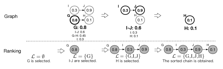
Figure 3: Example of the merging process performed in Algorithm 2, showing the merging of the two sub-chains $\text{G}\rightarrow\text{H}$ and $\text{I}\rightarrow\text{J}$ in Figure 2. The nodes indicated by bold circles correspond to the sub-chain of the highest mean scores, and the nodes indicated by gray-filled circles form the ranking produced by the merging procedure.

Theorem 5

Suppose Algorithm 1 is applied to an arbitrary sub-tree in $\operatorname*{\mathcal{G}}$, obtaining $\operatorname*{\mathcal{G}}^{\prime}$; i.e., the sub-tree is converted into a single chain. Then an optimal topological ordering of $\operatorname*{\mathcal{G}}^{\prime}$ is also an optimal topological ordering of $\operatorname*{\mathcal{G}}$. Hence, Algorithm 1 leads to an optimal topological ordering by merging all of the trees into a single chain.

The proof is given in Appendix E.2.

We have two remarks regarding HierRank. First, the time complexity of HierRank is $\operatorname*{\mathcal{O}}(K^{3})$ for each individual. It implies that the ranking over the $K$ nodes across $M$ individuals has a computational cost of $\operatorname*{\mathcal{O}}(MK^{3}+MK\log M)$. We can derive a faster version of the algorithm by eliminating the exhaustive merging and repeated computations performed at each iteration in HierRank; the computational cost for this version is $\operatorname*{\mathcal{O}}(n\log n)$ ($n=MK$). The details of this faster version, Algorithm 1^′, are given in Appendix B.3. Second, the current version of HierRank is designed for application to a tree graph. We can extend it for application to a DAG; the details of this version of the algorithm are given in Appendix B.4.

4.3 Procedure for Ranking Estimated mLPRs with Cutoff Selection

In this section, we place the mLPR estimation process and the ranking algorithm in the context of a unified procedure. We also provide a cutoff selection method for making a final decision based on the resulting ranking. The inputs to this procedure consist of a hierarchical graph and a data set that contains class-wise classifier scores and true labels; the outputs are a ranking and a cutoff value for this ranking. The procedure is as follows:

1. Split the data set into a training subset, a validation subset, and a testing subset.

2. Train models on the training data set for the estimation of mLPRs as described in Section 4.1, including training models or getting parameters for the estimations of LPRs, $\{\operatorname*{\mathbb{P}}(Y_{i})\}_{i=1,\ldots,n}$, $\{\operatorname*{\mathbb{P}}(Y_{i}|\operatorname*{\boldsymbol{Y}}_{pa(i)})\}_{i=1,ldots,n}$.

3. Estimate mLPRs on the validation data set and the testing data set.

4. Apply HierRank (Algorithm 1) to rank the $\widehat{mLPR}$ values on the validation data set (producing one ranking) and the testing data set (producing another ranking).

5. Compute a metric of interest (e.g., false discovery proportion (FDP), defined as the ratio of # of false positives over # of discoveries, or $F_{1}$ score, defined as the harmonic mean of the recall and the precision) at every cutoff value (e.g., top $10\times 100\%$) for the ranking on the validation data set. Then, select the cutoff value to optimize that metric as desired (e.g., targeting a specific FDR value or maximizing the $F_{1}$ score).

6. Apply the selected cutoff value to the ranking obtained with the testing data set.

The empirical performance of the cutoff selection procedure (Steps 4–5) was examined using a synthetic data set; see Section 5.2. On the other hand, we can provide a theoretical justification for this procedure: the naive ranking of mLPRs achieves Bayes optimality with respect to the top-$l$ error under certain conditions. We refer interested readers to Appendix C for a detailed discussion.

5 Experiments

We compared our method with off-the-shelf HMC approaches on one synthetic data set and two real data sets. We performed the evaluation using two criteria, described below.

5.1 Setup

Methods Compared. We evaluated our method in a comparison with several competitors, listed below. Details of these methods are summarized in Table S1 in Appendix D.3.

• Raw [score]–based methods. The raw classifier scores are ranked by NaiveSort and HierRank, which we call Raw-NaiveSort and Raw-HierRank, respectively.

• Clus-HMC variants. Clus-HMC is a state-of-the-art global HMC classifier (Blockeel et al., 2002, 2006; Vens et al., 2008) that performs classification and solves the hierarchy issue simultaneously. We used the R package Clus to implement two versions of Clus-HMC: one version with bagging, which we call ClusHMC-bagging, and the other version without ensembles, which we call ClusHMC-vanilla.

• HIROM variants. HIROM is a state-of-the-art local HMC classifier (Bi and Kwok, 2015) and produces Bayes-optimal predictions that minimize a series of hierarchical risks, such as risks based on hierarchical ranking loss and hierarchical Hamming loss. We implemented these two variants called HIROM-hier.ranking and HIROM-hier.Hamming, respectively.

• $\widehat{mLPR}$-based methods. Our method, $\widehat{mLPR}$-HierRank, which estimates mLPRs and ranks $\widehat{mLPR}$ values using HierRank, was implemented in an R package. $\widehat{mLPR}$ values can also be ranked by NaiveSort; we call this method $\widehat{mLPR}$-NaiveSort. We add postfixes “-indpt”, “-nbh”, “-full” to either method (e.g., $\widehat{mLPR}$-HierRank-full) to distinguish the independence approximation, the neighborhood approximation, and the full version for performing mLPR estimation, as described in Section 4.1

Evaluation Criteria. We used the below two criteria to evaluate ranking results produced by the aforementioned methods.

• Evaluation Criterion I: Precision–Recall curve. We used the PR curve to evaluate each ranking (produced by any of the methods listed above) from a holistic perspective. We further assessed the ranking by computing recall (i.e., # true discoveries / # all true positives) and precision (i.e., # true discoveries /# discoveries) values up to the top $\kappa\times 100\%$ events, where $\kappa$ := {# of top events that were taken as discoveries}/{total # of events}.

• Evaluation Criterion II: False discovery proportion (FDP)/$F_{1}$ score under proposed cutoff selection. We employed the procedure introduced in Section 4.3 to determine the cutoff value for the resulting ranking. Then, we evaluated this ranking along with the cutoff value selected on the validation set in terms of the maximal $F_{1}$ score and the FDP value whose associated target FDR was taken at the level $\alpha\times 100\%$ for $\alpha$ values of 0.01, 0.05, 0.1, and 0.2.

Data Sets. Each HMC method was evaluated using three data sets: 1) a synthetic data set, 2) the disease diagnosis data set from Huang et al. (2010), and 3) the RCV1v2 data set (Lewis et al., 2004). Details of these data sets are given below.

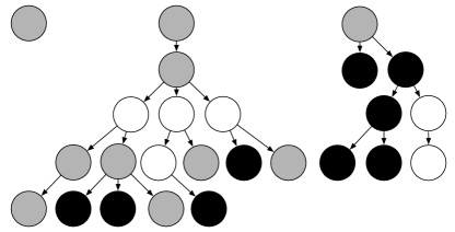
Figure 4: Structure of the synthetic data set. White, gray, and black correspond to high, medium, and low quality, respectively.

• Synthetic data set. The simulated data set consisted of 25 classes, whose hierarchy is shown in Figure 4. There were 50,000 training samples and 10,000 testing samples. For each sample, we generated the true instance status as follows. The root probability $\operatorname*{\mathbb{P}}(Y_{\text{root}}=1)$ and the conditional probabilities $\operatorname*{\mathbb{P}}(Y_{i}=1|\operatorname*{\boldsymbol{Y}}_{pa(i)}=1)$ were randomly generated from a uniform distribution, with the constraint that there had to be a minimum of 15 positive instances for any class in the training set (i.e., a minimum prevalence of $0.3\%$). Given the true instance status, the score $S$ was generated from status-specific distributions: data were generated from a Beta($\eta$, 3.5) distribution for the negative case and a Beta(3.5, $\eta$) distribution for the positive case. Here, we set $\eta$ to 2, 5.5 or 4 in descending order of the absolute mean difference between the two Beta distributions (i.e., $|3.5-\eta|/|3.5+\eta|$), corresponding to the high, medium, or low node quality, respectively. The quality of a node refers to the difficulty in distinguishing between the positives and the negatives. Specifics of the score generation mechanism are summarized in Table 1.

  Quality	Positive instance	Negative instance	Absolute mean difference	Node color
  High	Beta$(3.5,2)$	Beta$(2,3.5)$	$3/11$	white
  Medium	Beta$(3.5,5.5)$	Beta$(5.5,3.5)$	$2/9$	gray
  Low	Beta$(3.5,4)$	Beta$(4,3.5)$	$1/15$	black

  Table 1: Score distributions by node quality for synthetic data set.

• Disease diagnosis data set. Huang et al. (2010) studied the disease diagnosis problem using the UMLS directed acyclic graph and public microarray data sets from the National Center for Biotechnology Information (NCBI) Gene Expression Omnibus (GEO). They collected data from 100 studies, including a total of 196 data sets and 110 disease classes. The 110 classes represent 110 nodes, which are grouped into 24 connected DAGs (Figure 5); see Appendix D.2 for further detail. In general, this graph has three properties:

  1. It is shallow rather than deep.

  2. It is scattered rather than highly connected.

  3. Data redundancy occurs, e.g., for some nodes, all of the positive instances are also positive for the associated child nodes.

  

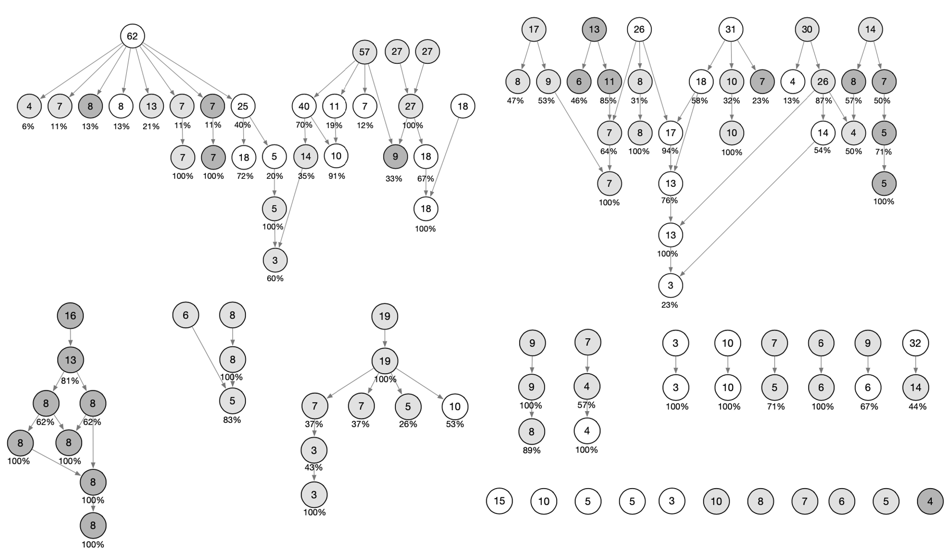
  Figure 5: Structure of the classes of the disease diagnosis data set. The grayscale corresponds to node quality: white indicates that a node’s base classifier has an area under the curve (AUC) value of receiver operating characteristic curve (ROC) within the interval $(0.9,1]$; light gray, $(0.7,0.9]$; and dark gray, $(0,0.7]$. The values inside the circles indicate the number of positive cases, and the values underneath indicate the maximum percentage of positive cases shared with a parent node.

• RCV1v2. This is the Reuters Corpus Volume I (RCV1) data set, which we included as the basis for a text categorization task. The raw data contains $800,000$ manually categorized newswire stories. In this study, we used the corrected version RCV1v2, which contains $30,000$ samples in total and $103$ categories. These categories are grouped into four trees representing four groups: corporate/industrial, containing $34$ classes; economics, containing $26$ classes; government/social, containing $11$ classes; and markets, containing $32$ classes. The hierarchy for RCV1v2 and other details can be found in Lewis et al. (2004).

5.2 Results on Synthetic Data Set

Here, we report only the results using the full version for obtaining $\widehat{mLPR}$ because of its superiority in this example over the other two versions; more results are reported in Appendix D.4.

Results Based on Evaluation Criterion I. For each method, we followed Steps 1-3 of the procedure (with no consideration of a validation subset) given in Section 4.3 to obtain the ranking of the events in the testing data set. We took the top $\kappa\times 100\%$ events as discoveries and computed the corresponding precision and recall values for $\kappa$ values of 0.05, 0.1, 0.2, 0.3, and 0.5. From the results, shown in Table 2, we make the following observations.

1. The performance of $\widehat{mLPR}$-NaiveSort was nearly the same as that of $\widehat{mLPR}$-HierRank, and both outperformed the other methods. A possible reason is that a full consideration of the hierarchical information (using the full version of the procedure) and a large training sample size combine to produce $\widehat{mLPR}$ values very close to the true mLPRs. In this scenario, NaiveSort and HierRank lead to similar rankings according to Proposition 1, and these rankings should be nearly optimal in terms of CATCH, according to Section 3.3.

2. Raw-NaiveSort and Raw-HierRank were much inferior to the other methods; however, the latter outperformed the former to a remarkable degree. They performed poorly because raw scores are output by class-specific classifiers, without accounting for hierarchical information as do the versions for obtaining $\widehat{mLPR}$ values. They differed in their performance because directly sorting raw scores via NaiveSort might violate the hierarchy, whereas HierRank produces a ranking that respects the hierarchy. In general, HierRank will never perform worse than NaiveSort.

$\kappa~{}$	0.05		0.1		0.2		0.3		0.5
Method	recall	prec	recall	prec	recall	prec	recall	prec	recall	prec
Raw-NaiveSort	5.3	13.9	8.5	11.2	14.0	19.2	20.2	8.9	35.4	9.3
Raw-HierRank	5.1	13.5	13.5	17.8	30.4	20.0	45.5	20.0	69.1	18.2
ClusHMC-vanilla	32.7	86.2	54.4	73.0	76.6	50.5	85.8	37.7	93.9	24.8
ClusHMC-bagging	33.9	89.3	56.7	74.7	76.8	50.6	86.5	38.0	94.3	24.9
HIROM-hier.ranking	35.5	93.5	55.6	81.0	81.1	53.5	84.1	36.9	88.7	23.4
HIROM-hier.Hamming	35.7	94.2	59.7	78.8	85.4	56.3	89.6	39.4	92.6	24.4
$\widehat{mLPR}$-NaiveSort-full	36.6	96.6	64.7	85.3	86.8	57.2	93.9	41.3	98.6	26.0
$\widehat{mLPR}$-HierRank-full	36.6	96.6	64.7	85.3	86.8	57.2	93.9	41.3	98.7	26.0

Table 2: Recall and precision (“prec”) values on the synthetic data. Here, $\kappa:=\text{\{\# of top events that were taken as discoveries\}/\{total \# of events\}}$. The highest values in each column are in bold. All values are percentages.

Results Based on Evaluation Criterion II. We split the original testing data set equally into a validation set and a new testing data set ($5,000$ samples in each), and then followed Steps 1-5 of the procedure in Section 4.3 to obtain a cutoff value for the ranking on the new testing data set. The corresponding discovery proportion ($:=$ {# of discoveries}/{total # of events}), the observed FDP, and the $F_{1}$ score obtained were computed and are summarized in Tables 3 and 4. As can be seen in Table 3, $\widehat{mLPR}$-HierRank-full made the most discoveries while controlling the FDP. Table 4 shows that $\widehat{mLPR}$-HierRank-full achieved the highest $F_{1}$ score and the lowest FDP. Additionally, Table 3 shows that the FDP obtained was close to the target FDR (i.e., $\alpha$) for every method except Raw-NaiveSort and Raw-HierRank. We also observe (from the results shown in Table S4 in Appendix D.4) that the obtained $F_{1}$ score nearly reached the highest possible $F_{1}$ score for the corresponding ranking. As can be seen by these results, the strategy given in Section 4.3 produced a satisfactory cutoff as expected.

Target $\alpha\times 100$	1.0		5.0		10.0		20.0
Method	d.p.	FDP	d.p.	FDP	d.p.	FDP	d.p.	FDP
Raw-NaiveSort	0.002	0.0	0.002	0.0	0.026	31.3	0.032	37.5
Raw-HierRank	0.002	0.0	0.005	5.1	0.1	9.5	1.0	19.5
ClusHMC-vanilla	0.007	0.0	0.007	0.0	3.5	9.7	7.5	19.2
ClusHMC-bagging	0.002	0.0	2.2	5.1	4.6	9.6	8.4	19.6
HIROM-hier.ranking	0.02	0.0	2.9	5.1	6.2	9.7	10.3	19.0
HIROM-hier.Hamming	0.3	3.5	4.6	5.1	6.3	9.5	8.3	19.5
$\widehat{mLPR}$-NaiveSort-full	2.7	0.6	5.8	4.4	8.3	9.6	11.5	19.4
$\widehat{mLPR}$-HierRank-full	2.7	0.6	5.8	4.4	8.3	9.6	11.7	19.5

Table 3: Observed false discovery proportion (FDP) on the synthetic testing data set, which was obtained by applying the cutoff value selected to aim at a target FDR on the validation data set as the strategy in Section 4.3. Here, $\alpha$ is the significance level targeted by the strategy to control the FDR on the validation data set. Discovery proportion (“d.p.”) $:=\text{\{\# of discoveries\}/\{total \# of events\}}$. The highest values in each d.p. column are in bold. All values are percentages.

Method	d.p.	FDP	$F_{1}$ score
Raw-NaiveSort	98.9	86.7	29.0
Raw-HierRank	41.1	81.0	23.3
ClusHMC-vanilla	14.9	37.5	64.3
ClusHMC-bagging	11.6	27.2	66.5
HIROM-hier.ranking	13.6	27.6	73.2
HIROM-hier.Hamming	14.9	32.0	71.9
$\widehat{mLPR}$-NaiveSort-full	12.8	23.9	74.8
$\widehat{mLPR}$-HierRank-full	12.8	23.9	74.9

Table 4: $F_{1}$ score on the synthetic testing data set, which was obtained by applying the cutoff value to maximize the $F_{1}$ score on the validation data set as the strategy introduced in Section 4.3. The corresponding FDP is also reported. Discovery proportion (“d.p.”) $:=\text{\{\# of discoveries\}/\{total \# of events\}}$. The lowest FDP and the highest $F_{1}$ score are in bold. All values are percentages.

5.3 Results on Disease Diagnosis Data Set

For the assessment using the disease diagnosis data set, we followed the same training procedure used in Huang et al. (2010) to obtain the binary Bayesian classifiers. Specifically, we used leave-one-out cross-validation (LOOCV) to obtain the Bayesian classification scores for each sample. The other methods were executed in the same LOOCV fashion to allow a fair comparison. For this data set, we report on all three versions of the mLPR estimation procedure.

For each method, we plotted the PR curve for the resulting ranking. In Figure 6 (a), we note that the independence (indpt) approximation outperformed both the neighborhood (nbh) approximation and the full version. This result is attributed to the challenge of estimating the dependency using a data set with a low signal-to-noise ratio and small sample size. Thus, although the full version and the neighborhood approximation are theoretically better, in this case we prefer the independence approximation for its practical robustness. In addition, we observe that HierRank produced a better ranking than NaiveSort for each version of the mLPR estimation. This corroborates our previous conclusion that HierRank provides a better ranking than NaiveSort when the input scores are deficient (e.g., the $\widehat{mLPR}$ values are imperfect).

As shown in Figure 6 (b), $\widehat{mLPR}$-HierRank-indpt performed better than all of the other methods, and it performed noticeably better when the recall value was low (in the initial portion of the ranking). This result suggests that our method may be more desirable for applications such as disease diagnosis, in which the correctness of the top decisions is highly valued.

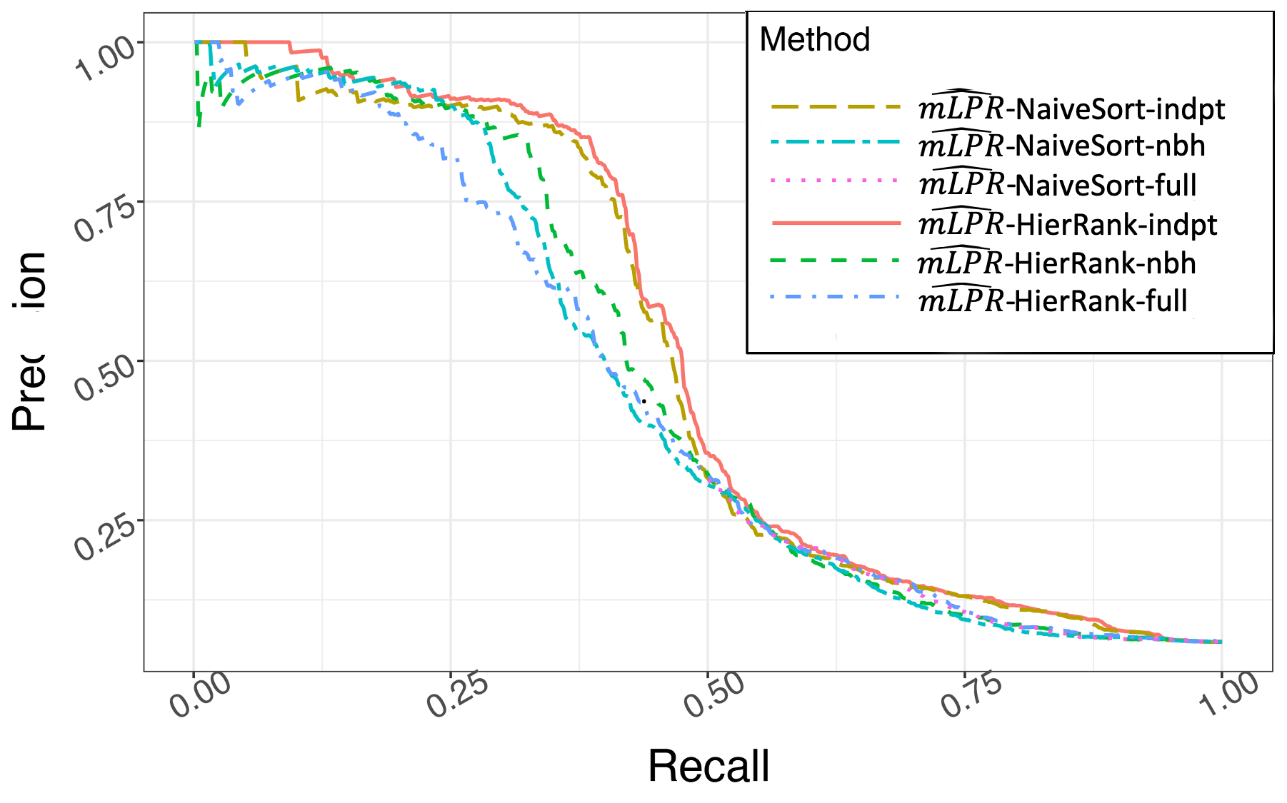
(a) Variants of $\widehat{mLPR}$-based methods

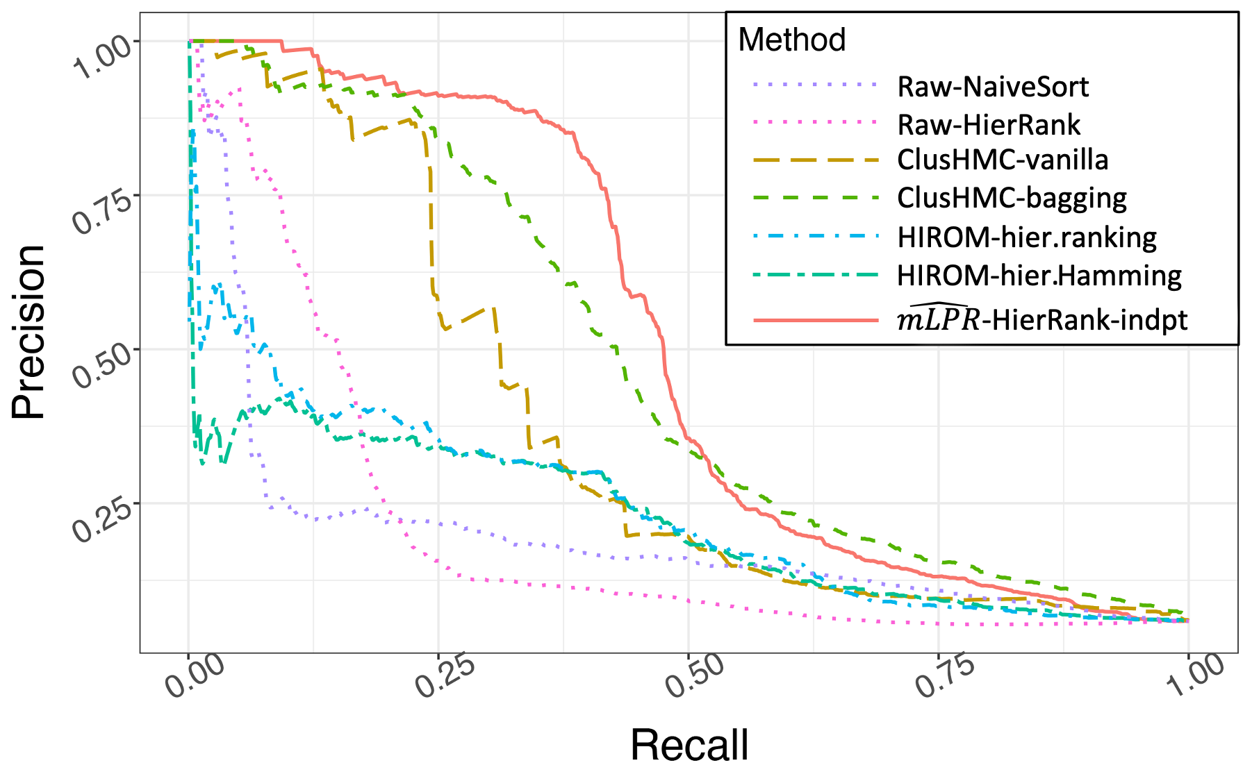
(b) All methods

Figure 6: Precision–recall curve for several classifiers applied to the disease diagnosis data set of Huang et al. (2010).

5.4 Results on RCV1v2 Data Set

For the analysis using RCV1v2, we split the training data set into two subsets, one for each stage of our method. Specifically, we trained class-wise support vector machines (SVMs) on the first training subset; on the second training subset, we used the classifier scores output by the SVMs to train models for the mLPR estimation. This procedure mitigated an overfitting issue we noticed when conducting the training for both stages on the same data set—as the distributions of the classifier scores on the training data set are different from those on the testing data set, overfitting can occur if the models of the second stage are trained on the same training data set as the first stage. We offer a further discussion in Appendix D.6 for interested readers.

Using the above strategy and following Steps 1-3 of the procedure (with no consideration of a validation subset) given in Section 4.3, we computed precision and recall values for $\widehat{mLPR}$-HierRank and the comparison methods on the RCV1v2 data set; these are shown in Table 5 (We omit the results for $\kappa>0.3$ because all precision values fell below $0.1$). When $\kappa\leq 0.1$, the Raw-based and Clus-HMC–based methods were inferior to the HIROM variants and $\widehat{mLPR}$-based methods. When $0.2\leq\kappa\leq 0.3$, $\widehat{mLPR}$-based methods outperformed all of the other methods. In addition, we note that among the three versions used for mLPR estimation, the methods with neighborhood approximation and the full version for estimating $\widehat{mLPR}$ performed similarly regardless of the sorting method, and both were superior to the independence approximation. These results suggest that in order to obtain a good estimation of mLPRs on this data set, the hierarchical information should be taken into account, and the neighborhood approximation should suffice.

$\kappa~{}$	0.05		0.1		0.2		0.3
	recall	prec	recall	prec	recall	prec	recall	prec
Raw-NaiveSort	4.0	2.5	5.3	1.7	6.9	1.1	8.5	0.9
Raw-HierRank	7.3	4.6	11.1	3.5	17.5	2.8	23.6	2.5
ClusHMC-vanilla	68.5	43.2	80.0	25.2	88.2	13.9	90.8	9.5
ClusHMC-bagging	72.5	45.6	83.7	26.4	92.0	14.5	95.7	10.0
HIROM-hier.ranking	77.1	48.6	80.0	25.2	85.9	13.5	89.1	9.4
HIROM-hier.Hamming	75.4	47.5	88.8	28.0	91.7	14.4	93.8	9.8
$\widehat{mLPR}$-NaiveSort-indpt	74.9	47.2	85.8	27.0	92.4	14.5	94.4	9.9
$\widehat{mLPR}$-NaiveSort-nbh	77.8	49.0	88.8	28.0	93.5	14.7	97.0	10.2
$\widehat{mLPR}$-NaiveSort-full	77.5	48.8	88.9	28.0	93.9	14.8	96.8	10.2
$\widehat{mLPR}$-HierRank-indpt	75.8	47.9	86.6	27.3	92.7	14.6	95.2	10.0
$\widehat{mLPR}$-HierRank-nbh	78.0	49.1	88.9	28.0	94.1	14.7	96.5	10.2
$\widehat{mLPR}$-HierRank-full	77.5	48.8	88.9	28.0	93.6	14.8	97.0	10.1

Table 5: Recall and precision (“prec”) values for the rankings on the RCV1v2 data set. Here, $\kappa:=\text{\{\# of top events that were taken as discoveries\}/\{total \# of events\}}$. The highest values in each column are in bold. All values are percentages.

6 Discussion

In this article, we introduced the mLPR statistic and demonstrated that sorting the true mLPRs in descending order can achieve the optimal HMC performance in terms of CATCH while respecting the class hierarchy. In practice, true mLPRs are not accessible; therefore, we provided an approach for estimating mLPRs. We developed a ranking algorithm, HierRank, that leads to the highest $\widehat{CATCH}$ under the hierarchical constraint. Our method can be easily employed in varieties of HMC applications, including disease diagnosis, protein-function categorization, gene-function categorization, image classification, and text classification. Through extensive experiments, we found this approach to be superior to competing methods.

We considered three possible versions of the mLPR estimation procedure, which differ in the extent of their graph usage. We found that the full version is preferred when there are sufficient samples of good quality. In this situation, NaiveSort is nearly equivalent in performance to HierRank. When data quality is a major concern, we would recommend the independence or neighborhood approximation for the sake of robustness. In this scenario, HierRank can guarantee the hierarchy and boost performance. We point out that an analysis of selecting among the three versions from a theoretical perspective remains open to investigation.

Finally, there is room for improving this method. Although the $\widehat{mLPR}$-based methods provide good performance, their performance hinges on the given class-wise classifiers, which are not optimized under the hierarchy. The approach holds the promise of making a better end-to-end classification system that takes as input the raw data (covariates) and aims to maximize $CATCH\/$ given the graph hierarchy.

Appendix A Hit Curve

The hit curve has been explored in the information retrieval community as a useful alternative to the receiver operating characteristics (ROC) curve and the precision–recall (PR) curve. In a hit curve, the x-axis represents the number of discoveries, and the y-axis represents the number of true discoveries (i.e., the hit number); see Figure S1.

The hit curve is widely used in situations where the users are more interested in the top-ranked instances. For example, in evaluating the performance of a web search engine, the relevance of the top-ranked pages is more important than those that appear later in search results because users expect that the most relevant results appear first. The hit curve can serve well in this situation as a graphic representation of the ranker’s performance since it would plot the results in order of decreasing importance given by the ranker, and the y-axis would indicate the results’ relevance to the target.

In comparison, the ROC curve, which plots the true positive rates (TPRs) against the false positive rates (FPRs) at varying thresholds, does not depend on the prevalence of true positive instances (Davis and Goadrich, 2006; Hand, 2009). In the case of search results, the number of relevant pages is tiny compared to the size of the World Wide Web (i.e., low prevalence of true positive instances), which would result in an almost zero FPR for the top-ranked pages. That is to say, with very few true positives, the early part of the ROC curve would fail to visualize the search ranking performance meaningfully. In the case of many hierarchical multi-label classification problems, like the disease diagnosis problem, this issue exists as well: there are many candidate diseases to consider while few are relevant to the patient.

The PR curve is another counterpart of the hit curve. Although it accounts for prevalence to a degree (i.e., showing the trade-off between precision and recall at varying thresholds), it is less informative than the hit curve when there are very few true positives. Herskovic et al. (2007) provided a simple example where the hit curve can be the more informative choice: with only five true positive cases out of 1000, the hit curve’s shape clearly highlighted the call order of a method that had called 100 instances before the five true positives, whereas the corresponding PR curve was uninformative (i.e., both the recall and precision values were zero for the first 100 called instances).

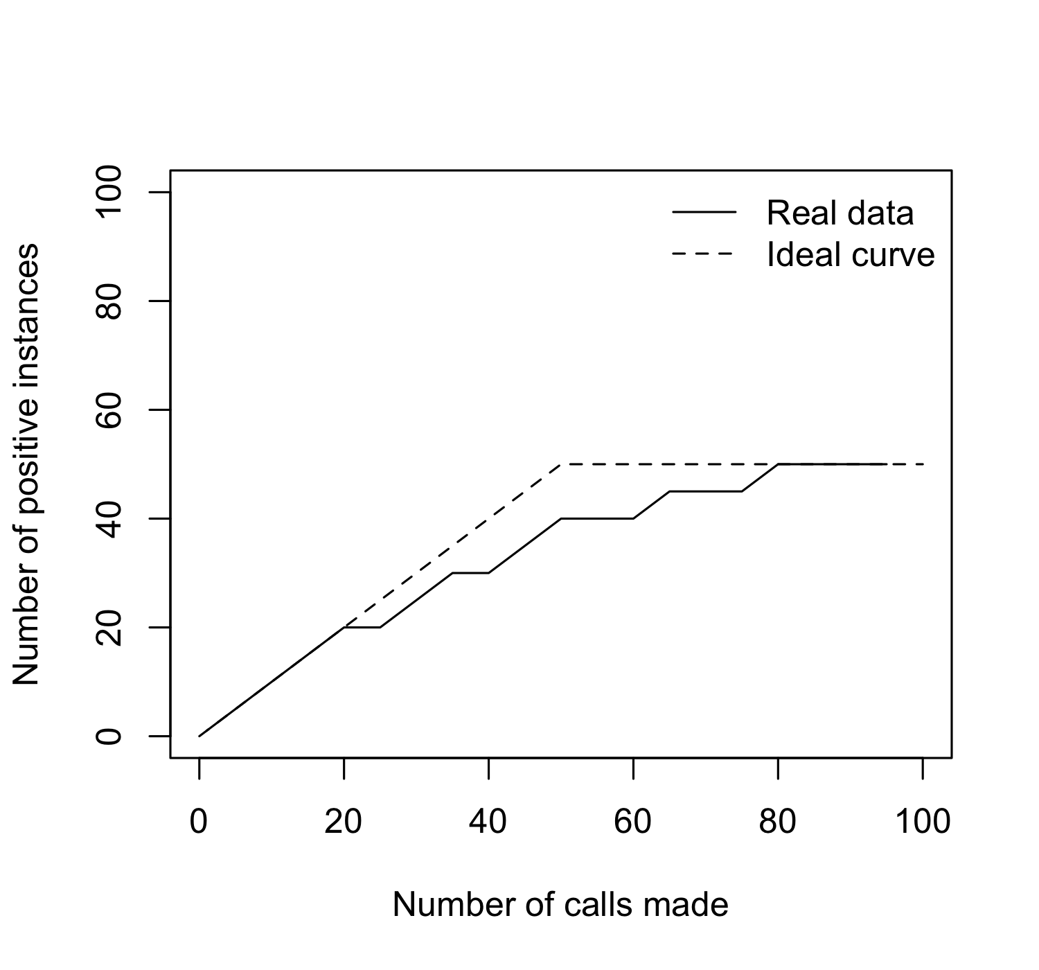
Figure S1: An example of a hit curve.

Appendix B Discussion on HierRank

We first give an example to illustrate HierRank. Then we discuss an existing algorithm that is similar to HierRank, and provide a faster implementation of HierRank. We conclude this section with an extension of HierRank to application of DAG.

B.1 Details of HierRank

We first consider ranking nodes from multiple disjoint single-child chains $\operatorname*{\mathcal{C}}_{r_{1}},\ldots,\operatorname*{\mathcal{C}}_{r_{p}}$. This procedure is equivalent to merging these chains into a single chain. The relative position along the resulting chain reflects the ranking. The corresponding method (Algorithm 2) is illustrated in Figure 3:

1. Initialize the ranked list $\operatorname*{\mathcal{L}}=\emptyset$.

2. For the chains $I\rightarrow J$ and $G\rightarrow H$, there are four sub-chains: $G$, $G\rightarrow H$, $I$, $I\rightarrow J$ with mean scores $0.8$, $0.45$, $0.3$, $0.6$ respectively. The sub-chain $G$ has the highest mean, so we remove it from the original graph and attach it to $\operatorname*{\mathcal{L}}$.

3. In the remaining graph, there are three sub-chains: $H$, $I$, and $I\rightarrow J$ with mean scores $0.1$, $0.3$, $0.6$. The sub-chain $I\rightarrow J$ has the highest mean, so we remove it from the remaining graph and attach it to $\operatorname*{\mathcal{L}}$.

4. There remains a single node $H$. We attach it to $\operatorname*{\mathcal{L}}$. Since there is no node in the remaining graph, $\operatorname*{\mathcal{L}}$ is the resulting ranking.

The produced ranking of Algorithm 2 satisfies the hierarchical consistency because it preserves the relative ordering of the nodes in each chain. This ranking also maximizes (4.2) since this algorithm essentially sorts the mean scores in descending order. The detailed argument is part of the proof of Theorem 5.

A general tree case corresponds to Algorithm 1 (HierRank), which uses Algorithm 2 repeatedly. Figure S2 is used to illustrate this algorithm:

1. Identify $\operatorname*{\mathcal{P}}_{1}$, $\operatorname*{\mathcal{P}}_{2}$ and $\operatorname*{\mathcal{P}}_{3}$. In Figure S2 (a), $\operatorname*{\mathcal{P}}_{1}=\{B,D,E,G,H,I,J,K,L\}$. $\operatorname*{\mathcal{P}}_{2}=\{F\}$, $\operatorname*{\mathcal{P}}_{3}=\{C\}$.

2. For each node in $\operatorname*{\mathcal{P}}_{2}$, we apply Algorithm 2 to merge the chains attached to it. Then attach the resulting single chain to this node, and update $\operatorname*{\mathcal{P}}_{1}$, $\operatorname*{\mathcal{P}}_{2}$, $\operatorname*{\mathcal{P}}_{3}$. In Figure S2 (a), $\operatorname*{\mathcal{P}}_{2}$ only contains Node $F$. Apply Algorithm 2 to merge the two sub-chains $G\rightarrow H$ and $I\rightarrow J$ attached to node $F$. Attach the resulting chain $G\rightarrow I\rightarrow J\rightarrow H$ to node F, and we get Figure S2 (b). Update $\operatorname*{\mathcal{P}}_{1}=\{B,D,E,C,F,G,I,J,H,K,L\}$, $\operatorname*{\mathcal{P}}_{2}=\{A\}$, $\operatorname*{\mathcal{P}}_{3}=\emptyset$.

3. Repeat step (b) until $\operatorname*{\mathcal{P}}_{2}$ is empty (then $\operatorname*{\mathcal{P}}_{3}$ is empty as well). In Figure S2 (b), $\operatorname*{\mathcal{P}}_{2}$ only contains node $A$. Apply Algorithm 2 to merge the two sub-chains $B\rightarrow D\rightarrow E$ and $C\rightarrow F\rightarrow G\rightarrow I\rightarrow J\rightarrow H$ that are attached to node $A$. Attach the resulting chain $C\rightarrow F\rightarrow G\rightarrow B\rightarrow D\rightarrow I\rightarrow J\rightarrow E\rightarrow H$ to node $A$, and we obtain Figure S2 (c). Update $\operatorname*{\mathcal{P}}_{1}=\{\text{all nodes}\}$, $\operatorname*{\mathcal{P}}_{2}=\emptyset$, $\operatorname*{\mathcal{P}}_{3}=\emptyset$. Since $\operatorname*{\mathcal{P}}_{2}$ is empty now, we terminate the loop.

4. Apply Algorithm 2 to merge the remaining single-child chains. In Figure S2 (c), there remain two sub-chains $K\rightarrow L$ and $A\rightarrow C\rightarrow F\rightarrow G\rightarrow B\rightarrow D\rightarrow I\rightarrow J\rightarrow E\rightarrow H$. Apply Algorithm 2 to merge them, and we obtain the resulting ranking $A\rightarrow K\rightarrow C\rightarrow F\rightarrow G\rightarrow B\rightarrow D\rightarrow I\rightarrow J\rightarrow L\rightarrow E\rightarrow H$.

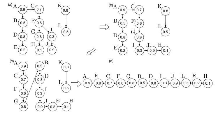
Figure S2: An example of the merging process in Algorithm 1: (a)$\rightarrow$(b) merge $G\rightarrow H$ and $I\rightarrow J$ into $G\rightarrow I\rightarrow J\rightarrow H$; (b)$\rightarrow$(c) merge $B\rightarrow D\rightarrow E$ and $C\rightarrow F\rightarrow G\rightarrow I\rightarrow J\rightarrow H$ to $C\rightarrow F\rightarrow G\rightarrow B\rightarrow D\rightarrow I\rightarrow J\rightarrow E\rightarrow H$; (c)$\rightarrow$(d) merge all nodes to $A\rightarrow K\rightarrow C\rightarrow F\rightarrow G\rightarrow B\rightarrow D\rightarrow I\rightarrow J\rightarrow L\rightarrow E\rightarrow H$.

B.2 An Almost Equivalent Algorithm

There is an existing algorithm called Condensing Sort and Select Algorithm (CSSA) (Baraniuk and Jones, 1994) that is of $\operatorname*{\mathcal{O}}(n\log n)$ complexity and can be adapted to solve (4.3). Bi and Kwok (2011) first extended CSSA in their proposed decision rule for the HMC problem. In their paper, CSSA was used to provide an approximate solution to the integer programming problem

$$\max_{\Psi} \sum_{k\in\mathcal{T}}B(k)\Psi(k)$$ (B.1)

$$s.t. \Psi(k)\in\{0,1\},\forall k;\quad\sum_{k\in\mathcal{T}}\Psi(k)=L,\Psi\text{ is }\mathcal{T}\text{-non-increasing}.$$ (B.2)

where $\mathcal{T}$-nonincreasing means that $\Phi(k)\leq\Phi(k^{\prime})$ if node $k^{\prime}$ is the ancestor of node $k$; $B(k)$ is some score to be ranked. Instead of directly solving (B.1) with (B.2), Bi and Kwok (2011) tackled a relaxed problem by replacing the binary constraint (B.2) with

$$0\leq\Psi(k)\leq 1,\forall k;\quad\Psi(0)=1,\sum_{k\in\mathcal{T}}\Psi(k)\leq L,\Psi\text{ is }\mathcal{T}\text{-non-increasing}.$$ (B.3)

Bi and Kwok (2011) proposed CSSA (Algorithm S1) to solve this problem. They showed that this algorithm can produce the optimal result that maximizes the objective function (B.1) while respecting (B.3) for each $L$.

Algorithm S1 The CSSA algorithm

Input: A collection of trees $\mathcal{T}$, scores $\operatorname*{\boldsymbol{S}}$ (e.g., $\widehat{mLPR}_{i}$’s)
Denote by $pa(T_{k})$ the parent of supernode $T_{k}$ that is a set of nodes, by $|T_{k}|$ the number of nodes in $T_{k}$, and by $\Psi$ a vector indicating which nodes are selected.

1:  Initialize $\Psi(0)\leftarrow 1$; $\Gamma\leftarrow 1$.

2:  Initialize all other nodes as supernodes with $\Psi(k)\leftarrow 0$ and sort them according to the scores.

3:  while $\Gamma<L$ do

4:     Find $k=\operatorname*{arg\,max}_{k^{\prime}}\sum_{i\in T_{k^{\prime}}}S_{i}/|T_{k^{\prime}}|$

5:     if $\Psi(pa(T_{k}))=1$ then

6:        $\Psi(T_{k})\leftarrow\min\{1,(L-\Gamma)/|T_{k}|\}$

7:        $\Gamma\leftarrow\Gamma+|T_{k}|$

8:     else

9:        Condense $T_{k}$ and $pa(T_{k})$ as a new supernode.

10:     end if

11:  end while

Output: Vector ${\bf\Psi}=(\Psi(1),\Psi(2),\ldots)$.

Note that CSSA has a property that $\Psi(k)=1$ for $L$ implies $\Psi(k)=1$ for $L^{\prime}$ (the same node $k$) when $L<L^{\prime}$. It implies this algorithm is able to produce a ranking by varying $L$. It turns out that CSSA can be modified as Algorithm S2 that is shown to generate almost the same result as HierRank (see Theorem S1; the proof is delegated to Appendix E.4). On the other hand, we note CSSA and Algorithm 1 differ in the following aspects.

Theorem S1

Algorithm 1 and Algorithm S2 yield the same ordering, except for local differences that lead to the same CATCH.

First, there might be local differences between the ranking of HierRank and that of CSSA. This results from the relaxation condition (B.3) — the same set of nodes can be selected for $L$ and $L+1$, thus CSSA cannot differentiate the ordering of some nodes. For example, consider a simple tree $B\leftarrow A\rightarrow C$, with $S_{B}=3.6$, $S_{A}=3$, $S_{C}=4$. In this case, $\Psi(A)=\Psi(B)=\Psi(C)=1/3$ when $L=1$; $\Psi(A)=\Psi(B)=\Psi(C)=2/3$ when $L=2$; $\Psi(A)=\Psi(B)=\Psi(C)=1$ when $L=3$. So Nodes $A$, $B$ and $C$ are always picked together. We only know that $A$ should be ranked ahead of $B$ and $C$, but cannot determine which of $B$ and $C$ should rank first. On the other hand, HierRank gives the resulting ranking $A\rightarrow C\rightarrow B$.

Second, HierRank is independently introduced and interpreted in the context of CATCH, with a statistical justification for ordering nodes using mLPRs in particular. CSSA originates in signal processing and has been successfully used in wavelet approximation and model-based compressed sensing (Baraniuk and Jones, 1994; Baraniuk, 1999; Baraniuk et al., 2010).

Finally, HierRank merges the chains from the bottom up, rather than, as in CSSA, constructing ordered sets of nodes called supernodes by starting from the node with the highest value in the graph and moving outward. It is easy to see that the block defined in Algorithm 1^′ (the faster version of HierRank introduced in Appendix B.3) is essentially the same as the supernode taken off in Algorithm S2. Hence, our independently proposed algorithm provides new insights into CSSA under the HMC setting.

Algorithm S2 An equivalent algorithm modified from CSSA.

Input: A forest $\mathcal{T}$, scores $\operatorname*{\boldsymbol{S}}$ (e.g., $\widehat{mLPR}_{i}$’s)
Denote by $pa(T_{k})$ the parent of supernode $T_{k}$ that is a set of nodes, by $|T_{k}|$ the number of nodes in $T_{k}$, and by $\operatorname*{\mathcal{L}}$ a vector for holding sorted scores.
Procedure:

1:  Initialize with one node per score value, and each node as its own supernode, $\operatorname*{\mathcal{L}}=[]$ (empty vector).

2:  while $|\operatorname*{\mathcal{L}}|<n$ do

3:     Find $k=\operatorname*{arg\,max}_{k^{\prime}}\sum_{i\in T_{k^{\prime}}}S_{i}/|T_{k^{\prime}}|$

4:     if $pa(T_{k})=\emptyset$ then

5:        Take the nodes in $T_{k}$ off the graph and append them to $\operatorname*{\mathcal{L}}$.

6:     else

7:        Condense $T_{k}$ and $pa(T_{k})$ into a supernode.

8:     end if

9:  end while

Output: A ranking $\operatorname*{\mathcal{L}}$.

B.3 A Faster Implementation of HierRank

To solve the scalability issue of Algorithm 1, we propose a faster version of HierRank by reducing redundant and repetitive computations in Algorithm 1. It is motivated by the following observations: 1) Algorithm 2 breaks a single chain into multiple blocks by identifying the point $(r^{\prime},h^{\prime})=\arg\underset{C_{r}(h)}{\max}\bar{\ell}_{\operatorname*{\boldsymbol{\tilde{S}}}}(r,h)$; 2) It can be shown that these blocks can only be agglomerated into a larger block rather than being further partitioned into smaller ones; 3) The agglomeration occurs only between a parent block and its child block in the hierarchy. Thus, HierRank can be implemented at the block level so that the partition is only executed once during multiple merging. By considering the above facts and taking care of other details, we obtain a faster version of HierRank (Algorithm 1^′), which costs $\operatorname*{\mathcal{O}}(n\log n)$ computations.

In Algorithm 2, we note the fact that each sub-chain in the tree can be partitioned into multiple blocks — given a chain $C_{r}$, the breaking points are sequentially defined as

$$p_{j}:=\left\{\begin{array}[]{ll}\max_{1\leq h\leq|C_{r}|}\frac{1}{|C_{r}(h)|}\sum_{k\in C_{r}(h)}S_{k},&\text{~{}if~{}}j==1;\\ \max_{p_{j-1}<h\leq|C_{r}|}\frac{\sum_{k\in C_{r}(h)/C_{r}(p_{j-1})}S_{k}}{|C_{r}(h)|-|C_{r}(p_{j-1})|},&\text{~{}if~{}}j>1.\\ \end{array}\right.$$ (B.4)

For example, Figure S3 (i) shows a chain of $6$ nodes can be partitioned into two blocks. During the merging procedure of Algorithm 1, it turns out that the blocks defined by the above partitions will not be broken into smaller pieces but can be further agglomerated. To show this, suppose there are two consecutive blocks in a chain, $B_{1}$, $B_{2}$, and $B_{1}$ locates ahead of $B_{2}$. Now we reform the blocks from the nodes in $B_{1}$ and $B_{2}$, using the rule in (B.4). It is obvious that nodes in $B_{1}$ will be clustered together. It remains to see which nodes in $B_{2}$ will be clustered with the nodes in $B_{1}$. Denote by $B_{2}(h)$ a sub-block consisting of the first $h$ nodes in $B_{2}$, and by $\bar{\ell}_{\operatorname*{\boldsymbol{\tilde{S}}}}(B)=\sum_{k\in B}S_{k}/|B|$ given a block $B$ and scores $\operatorname*{\boldsymbol{\tilde{S}}}$. For the sake of simplicity, we use $\bar{\ell}(B)$ for $\bar{\ell}_{\operatorname*{\boldsymbol{\tilde{S}}}}(B)$ when there is no confusion. Then, the mean scores of the nodes in $B_{1}$ and the first $h$ nodes in $B_{2}$ is computed as:

$$\bar{\ell}(B_{1}\cup B_{2}(h)) = \frac{|B_{1}|\bar{\ell}(B_{1})+h\bar{\ell}(B_{2}(h))}{|B_{1}|+h}=\bar{\ell}(B_{1})+\frac{\bar{\ell}(B_{2}(h))-\bar{\ell}(B_{1})}{|B_{1}|/h+1}.$$ (B.5)

By the definition of block $B_{2}$, we have $\bar{\ell}(B_{2})\geq\bar{\ell}(B_{2}(h))$, $\forall h=1,\ldots,|B_{2}|$. If $\bar{\ell}(B_{1})>\bar{\ell}(B_{2})$, none of the nodes in $B_{2}$ will be clustered together with the nodes in $B_{1}$. If $\bar{\ell}(B_{1})\leq\bar{\ell}(B_{2})$, (B.5) shows that all the nodes of $B_{1}$ and $B_{2}$ will form a new block. Therefore, blocks will not be broken into pieces but can be further agglomerated. During the merging process of multiple chains whose roots have the same parent, no blocks will be agglomerated since the blocks are sorted in a descending way along the merged chain; for example, see the three descendant blocks of the bold block in Figure S3 (ii). On the contrary, blocks can be agglomerated with those from the parent chain. Figure S3 (iii) shows that after the chain merging, the blocks in the merged chain can be further agglomerated with the parent block (the bold one).

These observations motivate us to propose Algorithm 1^′, a faster version of Algorithm 1. We avoid repeatedly computing moving means by partitioning each chain into blocks, and storing the size and the mean of each block. Specifically, there are three new components we need for Algorithm 1^′:

• Detect breaking points. For a chain $C_{r}$, breaking points can be detected by (B.4). Many existing algorithms can be used to this end. For example, recursion leads to an $\operatorname*{\mathcal{O}}(|C_{r}|\log|C_{r}|)$ time complexity. Figure S3 (i) illustrates this step.

• Merge multiple chains with defined blocks. Merging $m$ multiple chains with detected blocks can be realized using the k-way merge algorithm. The time complexity is $\operatorname*{\mathcal{O}}(s\log m)$, where $s$ is the total number of blocks in these chains. Figure S3 (ii) illustrates this step using a tree of five blocks.

• Agglomerate the upstream chain and the downstream merged chain. For a node $v\in\operatorname*{\mathcal{P}}_{2}$, denote by $C^{(v)}$ the longest chain that ends with the node $v$ and whose nodes except for $v$ have only one child. Suppose the children of $v$ are $r_{1},\ldots,r_{H}$. Denote by $C_{v}$ the chain output by merging $C_{r_{1}},\ldots,C_{r_{H}}$ using the k-way merge algorithm. Denote the blocks of $C^{(v)}$ by $B_{1}^{(up)},\ldots,B_{s}^{(up)}$ and the blocks of $C_{v}$ by $B_{1}^{(down)},\ldots,B_{t}^{(down)}$. Algorithm S3 agglomerates the blocks of $C^{(v)}$ and $C_{v}$ with a time complexity of $\operatorname*{\mathcal{O}}(|C^{(v)}|+|C_{v}|)$. Figure S3 (iii) illustrates this step using the output of Figure S3 (ii).

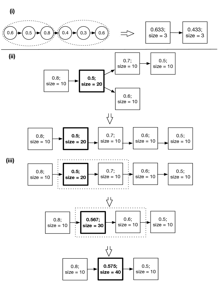
Figure S3: Illustrating the three components in Algorithm 1^′ using two examples which are separated by the solid line. The first example starts from a tree of six nodes, and the second example starts from a tree of five blocks. (i) Detect breaking points of the chain of six nodes and partition them into two blocks. (ii) Merge the two children chains of the bold block. (iii) Agglomerate the upstream chain and the downstream chain of the bold block. The blocks of the resulting list are positioned in a descending way.

Throughout Algorithm 1^′, the total time complexity consists of three parts: 1) detecting breaking points requires $\operatorname*{\mathcal{O}}(n\log K)$ computations; 2) merging multiple chains with defined blocks requires $\operatorname*{\mathcal{O}}(Dn\log K+n\log M)$ computations, where $D$ is the number of nodes that have multiple children in the graph (for one sample). The quantity $D$ upper bounds the number of times each sub-chain merges during the algorithm; 3) agglomerating the upstream chain and the downstream merged chain requires $\operatorname*{\mathcal{O}}(Dn)$ computations. In total, the time complexity of Algorithm 1^′ is $\operatorname*{\mathcal{O}}(Dn\log K)$. In reality, most tree structures are shallow with $D<10$. For example, the $D=5$ in Figure 5. So our algorithm is actually of $\operatorname*{\mathcal{O}}(n\log K)$ run time for practical use.

Algorithm S3 Agglomeration of blocks in the upstream chain and the downstream chain.

Input: Blocks $B_{1}^{(up)},\ldots,B_{s}^{(up)}$ from the upstream chain $C^{(v)}$ and Blocks $B_{1}^{(down)},\ldots,B_{t}^{(down)}$ from the downstream chain $C_{v}$.
Procedure:

1:  Let $b_{0}$ be $B_{1}^{(down)}$, $b_{-1}$ be the block ahead of $b_{0}$ in $C^{(v)}$ and $b_{+1}$ be the block after $b_{0}$ in $C_{v}$. Denote by $\bar{\ell}(b_{0}),\bar{\ell}(b_{-1}),\bar{\ell}(b_{+1})$ the mean scores within $b_{0}$, $b_{-1}$ and $b_{+1}$ respectively.

2:  while $\bar{\ell}(b_{0})>\bar{\ell}(b_{-1})$ or $\bar{\ell}(b_{+1})>\bar{\ell}(b_{0})$ do

3:     if $\bar{\ell}(b_{0})>\bar{\ell}(b_{-1})$ then

4:        Agglomerate $b_{0}$ and $b_{-1}$. The new block is still called $b_{0}$ and the block ahead of the original $b_{-1}$ now is called $b_{-1}$.

5:     else

6:        Agglomerate $b_{0}$ and $b_{+1}$. The new block is still called $b_{0}$ and the block after the original $b_{+1}$ now is called $b_{+1}$.

7:     end if

8:  end while

[1] Output: The new sequence of blocks.

Algorithm 1^′ A faster implementation of the HierRank algorithm.

Input: A forest $\mathcal{T}$, scores $\operatorname*{\boldsymbol{S}}$.
Procedure:

1:  Figure out $\operatorname*{\mathcal{P}}_{2}$.

2:  while $\operatorname*{\mathcal{P}}_{2}\neq\emptyset$ do

3:     Pop out a $v$ from $\operatorname*{\mathcal{P}}_{2}$. Take out all of its children $r_{1},\ldots,r_{H}$ (these children’s descendants have at most one child). Denote by $C^{(v)}$ the longest chain that ends with the node $v$ and whose nodes in $C^{(v)}$ except for $v$ have only one child.

4:     Find the breaking points $p_{1}^{(h)},\ldots,p_{S_{h}}^{(h)}$ for $C_{r_{h}}$ by (B.4), $h=1,\ldots,H$.

5:     Merge $C_{r_{1}},\ldots,C_{r_{H}}$, in terms of the mean score values of the blocks separated by the breaking points. Denote the new chain as $C_{v}$.

6:     Agglomerate blocks of $C^{(v)}$ and $C_{v}$ by Algorithm S3.

7:     Update $\operatorname*{\mathcal{P}}_{2}$.

8:  end while

9:  if There remain multiple chains then

10:     Merge them use the k-way merge algorithm.

11:  end if

12:  Let $\operatorname*{\mathcal{L}}$ be the resulting chain.

[1] Output: a ranking $\operatorname*{\mathcal{L}}$.

B.4 Extension to DAG

Directed acyclic graph (DAG) is a more general hierarchy than the tree structure and is more applicable to real data. In a DAG hierarchy structure, one node can have more than one parent, which brings about an additional decision issue – which parent the node and its descendants should respect. We call it the “AND” constraint if the node respects its all parents and call it the “OR” constraint if the node only respects one of its parents. Denote by $\operatorname*{\mathcal{Q}}$ all the nodes that have at least two parents.

It is easy to extend our algorithm for a tree hierarchy to a DAG structure by dynamic programming. For each node in $\operatorname*{\mathcal{Q}}$, we explore all the possible cases where this node respects one of its parents and disconnects the edges to other parents. Such a strategy obviously works for the “OR” constraint. Bi and Kwok (2011) has shown that at least one case satisfies the “AND” requirement. Each case boils down to a forest thus, we can use Algorithm 1^′ to get a ranking. For the “OR” requirement, we select the case with the highest objective function value. For the “AND” requirement, we select the scenario that attains the highest value among those that satisfy the requirement. Although the above brute-force strategy looks clumsy and time-consuming, it works for most practical scenarios since most applications have shallow and scattered hierarchy structures. For instance, in Figure 5, there are nine nodes that have multiple parents in a connected part. So we only need to explore $2^{7}=128$ cases at most. Considering there is only a limited number of labels, about $100$ most times, the computation time is acceptable.

To adapt HierRank to a complicated DAG with substantial nodes that have multiple parents, we follow the strategy used in CSSA. To be specific, we find the node $v$ with multiple parents and one of its parents has the minimal parent score value:

$$\text{Find }v\in\operatorname*{\mathcal{Q}}\text{ such that }\underset{u\in pa(v)}{\min}S_{u}=\underset{u\in\cup_{u^{\prime}\in\operatorname*{\mathcal{Q}}}pa(u^{\prime})}{\min}S_{u}.$$

Then we find the parent of $v$ that has the minimal score value:

$$\text{Find }u:=\underset{{u^{\prime}\in pa(v)}}{\operatorname*{arg\,min}}S_{u^{\prime}}.$$

Then we assign the parents of $v$ except for $u$ as the new parents of $u$ and disconnect $v$ to its parents but $u$. Bi and Kwok (2011) has shown that this strategy works for the “AND” constraint. The detailed algorithm that uses this strategy to extend HierRank to DAG is summarized as Algorithm S4. Similarly, by following the steps for the “OR” constraint in Bi and Kwok (2011), we can extend HierRank to DAG in this scenario.

Algorithm S4 The HierRank algorithm for the DAG hierarchy.

Input: The DAG graph $\operatorname*{\mathcal{G}}$, node scores $\operatorname*{\boldsymbol{S}}$.
Procedure:

1:  Figure out $\operatorname*{\mathcal{P}}_{2}$.

2:  Figure out $\operatorname*{\mathcal{Q}}:=\{v:v\text{ has more than one parent}\}$.

3:  while There is a node with more than one children or more than one parent. do

4:     while $\operatorname*{\mathcal{P}}_{2}\neq\emptyset$ do

5:        Pop out one $v$ from $\operatorname*{\mathcal{P}}_{2}$. Take two children of $v$, $r_{1}$ and $r_{2}$.

6:        Feed $C_{r_{1}}$ and $C_{r_{2}}$ into Algorithm 2 and obtain $\operatorname*{\mathcal{L}}(r_{1},r_{2})$.

7:        Replace $C_{r_{1}}$ and $C_{r_{2}}$ with $\operatorname*{\mathcal{L}}(r_{1},r_{2})$.

8:        Update $\operatorname*{\mathcal{P}}_{2}$.

9:     end while

10:     if $\operatorname*{\mathcal{Q}}\neq\emptyset$. then

11:        Find $v\in\operatorname*{\mathcal{Q}}$ such that $\underset{u\in pa(v)}{\min}S_{u}=\underset{u\in\cup_{u^{\prime}\in\operatorname*{\mathcal{Q}}}pa(u^{\prime})}{\min}S_{u}$. Find $u:=\underset{{u^{\prime}\in pa(v)}}{\operatorname*{arg\,min}}S_{u^{\prime}}$.

12:        Let $pa(u)=pa(u)\cup pa(v)/u$, $pa(v)=u$.

13:        Update $\operatorname*{\mathcal{P}}_{2}$ and $\operatorname*{\mathcal{Q}}$.

14:     end if

15:  end while

16:  if There remain multiple chains then

17:     Apply Algorithm 2 to these chains.

18:  end if

19:  Let $\operatorname*{\mathcal{L}}$ be the resulting chain.

[1] Output: a ranking $\operatorname*{\mathcal{L}}$.

Appendix C Bayes Optimality w.r.t Top-$l$ precision value

We look into the performance of the decision-making made based on the naive ranking of mLPRs. To this end, we consider a natural decision rule — take the events of the top $l$ mLPRs. Then we study the top-$l$ selection via a Bayes point-view. Specifically, we consider the risk function

$$R(\theta;err_{l})=\operatorname*{\mathbb{E}}_{(\operatorname*{\boldsymbol{x}},\operatorname*{\boldsymbol{y}})\sim P}[err_{l}(\theta(\operatorname*{\boldsymbol{x}}),\operatorname*{\boldsymbol{y}})],$$

where $(\operatorname*{\boldsymbol{x}},\operatorname*{\boldsymbol{y}})$ is assumed to be i.i.d generated from some distribution $P$; $\theta$ is a transformation function of the covariates $\operatorname*{\boldsymbol{x}}$; $err_{l}(\cdot,\cdot)$ is one minus top-$l$ precision value ($err_{l}:=\#\{\text{true negative events whose values are in the top $l$ list}\}/l$). We say $\theta^{*}$ is Bayes optimal w.r.t $err_{l}$ if

$$R(\theta^{*};err_{l})=\inf_{\theta}R(\theta;err_{l}).$$

We note that: 1) mLPR can be regarded as a function of $\operatorname*{\boldsymbol{x}}$ since it is a function of the first-stage classifier scores $\operatorname*{\boldsymbol{s}}$ that is a function of $\operatorname*{\boldsymbol{x}}$; 2) the precision value is equivalent to the hit number conditional on top-$l$ selection. Then the following result shows that mLPR satisfies Bayes optimality with respect to $err_{l}$ under some practically reasonable conditions.

Proposition S2

Suppose $\operatorname*{\mathbb{P}}(Y=1|\operatorname*{\boldsymbol{S}})$ has the top-$l$ preserving property (Yang and Koyejo, 2020), i.e., for all $k$,

$$\operatorname*{\mathbb{P}}(Y_{k}=1|\operatorname*{\boldsymbol{X}})>\operatorname*{\mathbb{P}}(Y_{[l+1]}=1|\operatorname*{\boldsymbol{X}})\Rightarrow\operatorname*{\mathbb{P}}(Y_{k}=1|\operatorname*{\boldsymbol{S}})>\operatorname*{\mathbb{P}}(Y_{[l+1]}=1|\operatorname*{\boldsymbol{S}}),$$

$$\operatorname*{\mathbb{P}}(Y_{k}=1|\operatorname*{\boldsymbol{X}})<\operatorname*{\mathbb{P}}(Y_{[l]}=1|\operatorname*{\boldsymbol{X}})\Rightarrow\operatorname*{\mathbb{P}}(Y_{k}=1|\operatorname*{\boldsymbol{S}})<\operatorname*{\mathbb{P}}(Y_{[l]}=1|\operatorname*{\boldsymbol{S}}),$$

where $[l]$ denotes the $l$-th highest value. Then, mLPR is Bayes optimal with respect to the $err_{l}$.

Proof  We first fix $\operatorname*{\boldsymbol{x}}$. Note that

$$\operatorname*{\mathbb{E}}_{\operatorname*{\boldsymbol{y}}\sim\operatorname*{\mathbb{P}}(Y|\operatorname*{\boldsymbol{X}}=\operatorname*{\boldsymbol{x}})}[err_{l}(\theta(\operatorname*{\boldsymbol{x}}),\operatorname*{\boldsymbol{y}})]=1-[\sum_{k:\theta(\operatorname*{\boldsymbol{x}})_{k}\geq\theta(\operatorname*{\boldsymbol{x}})_{[l]}}\operatorname*{\mathbb{P}}(Y_{k}=1|\operatorname*{\boldsymbol{X}}=\operatorname*{\boldsymbol{x}})]/l.$$

By Proposition 2.1 of Yang and Koyejo (2020), mLPR is top-$l$ Bayes optimal for any $l>0$.  

Remark S3

Note that the first-stage classifiers attempt to learn $S_{k}=\operatorname*{\mathbb{P}}(Y_{k}=1|\operatorname*{\boldsymbol{X}})$. So the condition of having the top-$l$ preserving property can be achieved when the first-stage classifiers are sufficiently good. For instance, assume $\operatorname*{\mathbb{P}}(\operatorname*{\boldsymbol{X}})$ to be a Gaussian mixture model $\operatorname*{\mathbb{P}}(\operatorname*{\boldsymbol{X}})=\sum_{k=1}^{K}\tau_{k}\cdot G(\operatorname*{\boldsymbol{X}};\boldsymbol{\mu}_{k},\boldsymbol{\Sigma}_{k})$, where $\tau_{k}=\operatorname*{\mathbb{P}}(Y_{k}=1)$, $\boldsymbol{\mu}_{k}$ and $\boldsymbol{\Sigma}_{k}$ are the mean and covariance matrix of the $k$-th component. Then the score $\operatorname*{\boldsymbol{S}}=(S_{1},\ldots,S_{K})$ is desired with $S_{k}=\phi(\operatorname*{\boldsymbol{X}};\boldsymbol{\mu}_{k},\boldsymbol{\Sigma}_{k})/[\sum_{k^{\prime}=1}^{K}\phi(\operatorname*{\boldsymbol{X}};\boldsymbol{\mu}_{k^{\prime}},\boldsymbol{\Sigma}_{k^{\prime}})]$, where $\phi(\operatorname*{\boldsymbol{X}};\boldsymbol{\mu}_{k},\boldsymbol{\Sigma}_{k})$ is the multivariate Gaussian density with mean $\boldsymbol{\mu}_{k}$ and covariance matrix $\boldsymbol{\Sigma}_{k}$. Such a score is a one-to-one transformation of the sufficient statistics $\boldsymbol{\mu}_{k}$, $\boldsymbol{\Sigma}_{k}$, $k=1,\ldots,K$, and it captures all the useful information for classification contained in $\operatorname*{\boldsymbol{X}}$.

Appendix D Experiments

Here, we provide more details and supplmentary results for Section 5.

D.1 Background of the Disease Data and the First-stage Classifiers

Huang et al. (2010) developed a classifier for predicting disease along the Unified Medical Language System (UMLS) directed acyclic graph, trained on public microarray data sets from the National Center for Biotechnology Information (NCBI) Gene Expression Omnibus (GEO). GEO was originally founded in 2000 to systematically catalog the growing volume of data produced in microarray gene expression studies. GEO data typically comes from research experiments where scientists are required to make their data available in a public repository by grant or journal guidelines. In July 2008, GEO contained 421 human gene expression studies on the three microarray platforms that were selected for analysis (Affymetrix HG-U95A (GPL91), HG-U133A (GPL96), and HG-U133 Plus 2 (GPL570)). In this study, 100 studies were collected, yielding a total of 196 data sets. These were used for training the classifier in Huang et al. (2010).

Labels for each data set were obtained by mapping text from descriptions on GEO to concepts in the UMLS. The mapping resulted in a directed acyclic graph of 110 concepts matched to the 196 data sets at two levels of similarity – a match at the GEO submission level, and a match at the data set level, with the latter being a stronger match. The disease concepts and their GEO matches are listed in Table S2 in the supplementary information for Huang et al. (2010).

Training a classifier for each label is a complex multi-step process and is described in detail in the Supplementary Information of Huang et al. (2010). We summarize that process here. In the classifier for a particular disease concept, the negative training instances were the profiles among the 196 that did not match with that disease concept. The principal modeling step involved expressing the posterior probability of belonging to a label in terms of the log-likelihood ratio and some probabilities that have straightforward empirical estimates. The log-likelihood ratio was modeled with a log-linear regression. A posterior probability estimate was then obtained for each of the 110 $\times$ 196 instances in the data by leave-one-out cross-validation, i.e., estimating the $i$-th posterior probability based on the remaining ones. These posterior probability estimates were used as the first-stage classifier scores.

D.2 Characteristics of the Disease Diagnosis Data and Hierarchy

The full hierarchy graph is shown in Figure 5. As the two figures show, the 110 nodes are grouped into 24 connected sets. In general, the graph is shallow rather than deep: the maximum node depth is 6, though the median is 2. Only ten nodes have more than one child. This occurs because 11 of the connected sets are standalone nodes, while six are simple two-node trees. The two largest sets consist of 28 and 30 nodes, respectively.

The graph nearly follows a tree structure. Most nodes have only one parent or are at the root level. Only 15 nodes have 2 parents, and 2 nodes have 3 parents. Most nodes do not have a high positive case prevalence. The biggest number of samples belonging to a label is 62, or a 32.63% positive case prevalence. The average prevalence is 5.89%, with a minimum prevalence of 1.53%, corresponding to 3 cases for a label. Data redundancy occurs as an artifact of the label mining: usually, the positive instances for a disease concept are the same as for its parents. There are few data sets that are tagged with a general label and not a leaf-level one. Twenty-six nodes or 23.64% of all nodes share the same data as their parents, so they have the same classifier and, therefore, the same classifier scores as their parents. If we take the number of nodes that share more than half of their data with their parent, this statistic rises to 50%. A consequence of this redundancy is that the graph is shallower than appears in the figure.

D.3 Details of Method Implementations on Each Data Set

Synthetic data set. For the synthetic data set, we used empirical proportions in the training data set to estimate $\operatorname*{\mathbb{P}}(Y_{i}|\operatorname*{\boldsymbol{\tilde{Y}}}_{pa(i)})$ and $\operatorname*{\mathbb{P}}(Y_{i})$, which were used to estimate mLPRs and learn HIROM.

Disease diagnosis. For the disease-diagnosis data set, we used the empirical proportion in the training data set to estimate $\operatorname*{\mathbb{P}}(Y_{i}|\operatorname*{\boldsymbol{\tilde{Y}}}_{pa(i)})$ and $\operatorname*{\mathbb{P}}(Y_{i})$ since the disease-diagnosis data has very limited sample size.

ClusHMC implementation on all data sets. We used ClusHMC and follow Dimitrovski et al. (2011) by constructing bagged ensembles and used the original settings of Vens et al. (2008), weighting each node equally when assessing distance, i.e. $w_{i}=1$ for all $i$. In addition to node weights, the minimum number of instances was set to 5, and the minimum variance reduction was tuned via 5-fold cross-validation from the options 0.60, 0.70, 0.80, 0.90, and 0.95. Following the implementation of Lee (2013), a default of 100 Predictive Clustering Trees (PCTs) were trained for each ClusHMC ensemble; each PCT was estimated by resampling the training data with replacement and running ClusHMC on the result.

Method	Raw-	ClusHMC-	HIROM-	$\widehat{mLPR}$-
Type	two-stage method (2nd stage)	global method	two-stage method (1st and 2nd stage)	two-stage method (2nd stage)
Input	Classifier Scores	Labels $Y_{i}$’s; Covariates	Labels $Y_{i}$’s; Covariates	Labels $Y_{i}$’s; Classifier Scores
Ranking	naive sorting, HierRank	N/A	HierRank	naive sorting, HierRank
Variants	N/A	version: vanilla, bagging	loss: Hier. Ranking, Hier. Hamming	Approximation: indpt, nbh, full

Table S1: Method details. “Raw-” stands for “Raw [score]–based methods”, “ClusHMC-” stands for “Clus-HMC variants”, “HIROM-” stands for “HIROM variants”, and “$\widehat{mLPR}$-” stands for “$\widehat{mLPR}$–based methods”.

D.4 Additional Results

Additional results for Section 5.2 are put in Table S2, S3, S4. For the $\widehat{mLPR}$–based methods, “Gaussian” corresponds to the variant that uses Formula (4.1) (b) to estimate mLPRs while “LPR” corresponds to the variant that uses Formula (4.1) (d).

$\kappa~{}$		0.05		0.1		0.2		0.3		0.5
Method		recall	prec	recall	prec	recall	prec	recall	prec	recall	prec
Raw	NaiveSort	5.3	13.9	8.5	11.2	14.0	19.2	20.2	8.9	35.4	9.3
	HierRank	5.1	13.5	13.5	17.8	30.4	20.0	45.5	20.0	69.1	18.2
ClusHMC	vanilla	32.7	86.2	54.4	73.0	76.6	50.5	85.8	37.7	93.9	24.8
	bagging	33.9	89.3	56.7	74.7	76.8	50.6	86.5	38.0	94.3	24.9
HIROM	hier.ranking	35.5	93.5	55.6	81.0	81.1	53.5	84.1	36.9	88.7	23.4
	hier.Hamming	35.7	94.2	59.7	78.8	85.4	56.3	89.6	39.4	92.6	24.4
$\widehat{mLPR}$-HierRank (Gaussian)	indpt	34.7	91.5	53.7	70.8	76.7	50.5	87.8	38.6	94.3	24.9
	nbh	34.0	89.7	59.8	78.8	81.7	53.8	89.5	39.3	95.3	25.1
	full	35.2	92.8	60.2	79.3	81.6	53.8	89.9	39.5	96.3	25.4
$\widehat{mLPR}$-NaiveSort (LPR)	indpt	35.5	93.6	60.7	80.0	82.2	54.2	89.2	39.2	95.6	25.2
	nbh	36.4	96.0	63.8	84.1	85.5	56.4	92.6	40.7	97.5	25.7
	full	36.6	96.6	64.7	85.3	86.8	57.2	93.9	41.3	98.6	26.0
$\widehat{mLPR}$-HierRank (LPR)	indpt	35.7	94.1	62.3	82.1	82.8	54.6	89.9	39.5	95.8	25.3
	nbh	36.5	96.2	64.0	84.4	85.7	56.5	92.8	40.8	97.6	25.7
	full	36.6	96.6	64.7	85.3	86.8	57.2	93.9	41.3	98.7	26.0

Table S2: The recall and precision values of the synthetic testing data. Here $\kappa:=\text{ratio of \# \{top events that were taken as discoveries\} to \# \{total events\}}$. The highest values are in bold in each column. All the values are in percentage.

Target $\alpha\times 100$		1.0		5.0		10.0		20.0
Method		d.p.	FDP	d.p.	FDP	d.p.	FDP	d.p.	FDP
Raw Scores	NaiveSort	0.002	0.0	0.002	0.0	0.026	31.3	0.032	37.5
	HierRank	0.002	0.0	0.005	5.1	0.1	9.5	1.0	19.5
ClusHMC	vanilla	0.007	0.0	0.007	0.0	3.5	9.7	7.5	19.2
	bagging	0.002	0.0	2.2	5.1	4.6	9.6	8.4	19.6
HIROM	hier.ranking	0.02	0.0	2.9	5.1	6.2	9.7	10.3	19.0
	hier.Hamming	0.3	3.5	4.6	5.1	6.3	9.5	8.3	19.5
$\widehat{mLPR}$-HierRank (Gaussian)	indpt	1.3	1.5	3.8	5.1	5.4	9.6	8.0	19.5
	nbh	1.9	1.3	3.3	4.7	4.7	9.8	9.4	19.1
	full	2.2	1.1	4.2	5.0	6.0	9.9	9.7	19.4
$\widehat{mLPR}$-NaiveSort (LPR)	indpt	1.3	1.1	4.4	5.0	7.0	9.2	10.5	18.8
	nbh	2.4	0.8	5.7	4.7	8.0	9.3	11.2	19.1
	full	2.7	0.6	5.8	4.4	8.3	9.6	11.5	19.4
$\widehat{mLPR}$-HierRank (LPR)	indpt	1.5	1.3	4.1	4.6	6.4	9.3	9.9	19.7
	nbh	2.5	0.8	5.6	4.6	7.9	9.5	11.1	19.3
	full	2.7	0.6	5.8	4.4	8.3	9.6	11.7	19.5

Table S3: The observed FDP on the synthetic testing data set, which obtained by the strategy in Section 4.3. Here $\alpha$ is the significance level at which the strategy targets to control the FDR on the validation data set. The “d.p.” column refers to discovery proportion $:=\text{\# discoveries/\# \{total events\}}$. The highest values are in bold in each d.p. column. All the values are in percentage.

Method		d.p.	FDP	obtained F-score	maximal F-score
Raw Scores	NaiveSort	98.9	86.7	29.0	29.1
	HierRank	41.1	81.0	23.3	23.3
ClusHMC	vanilla	14.9	37.5	64.3	64.4
	bagging	11.6	27.2	66.5	66.6
HIROM	hier.ranking	13.6	27.6	73.2	73.2
	hier.Hamming	14.9	32.0	71.9	72.0
$\widehat{mLPR}$-HierRank (Gaussian)	indpt	18.1	46.7	61.4	61.5
	nbh	12.9	28.8	70.2	70.2
	full	13.7	28.1	70.1	70.2
$\widehat{mLPR}$-NaiveSort (LPR)	indpt	12.2	30.6	70.4	70.4
	nbh	12.4	24.4	73.9	73.9
	full	12.8	23.9	74.8	74.9
$\widehat{mLPR}$-HierRank (LPR)	indpt	11.9	23.5	71.4	71.5
	nbh	12.4	24.0	74.2	74.2
	full	12.8	23.9	74.9	75.0

Table S4: The $F_{1}$-score on the synthetic testing data set, obtained by the strategy introduced in Section 4.3. The corresponding FDP is reported. The “d.p.” column refers to discovery proportion $:=\text{\# discoveries/\# \{total events\}}$. The highest $F_{1}$-score and the lowest FDP are in bold. All the values are in percentage.

D.5 Discussion of Statistical Differences Between Classes

Figure S4 is an example based on the SVM values for two classes of the RCV1v2 data set in Section 5.4, which shows ignorance of the statistical difference between classes can lead to a bad decision.

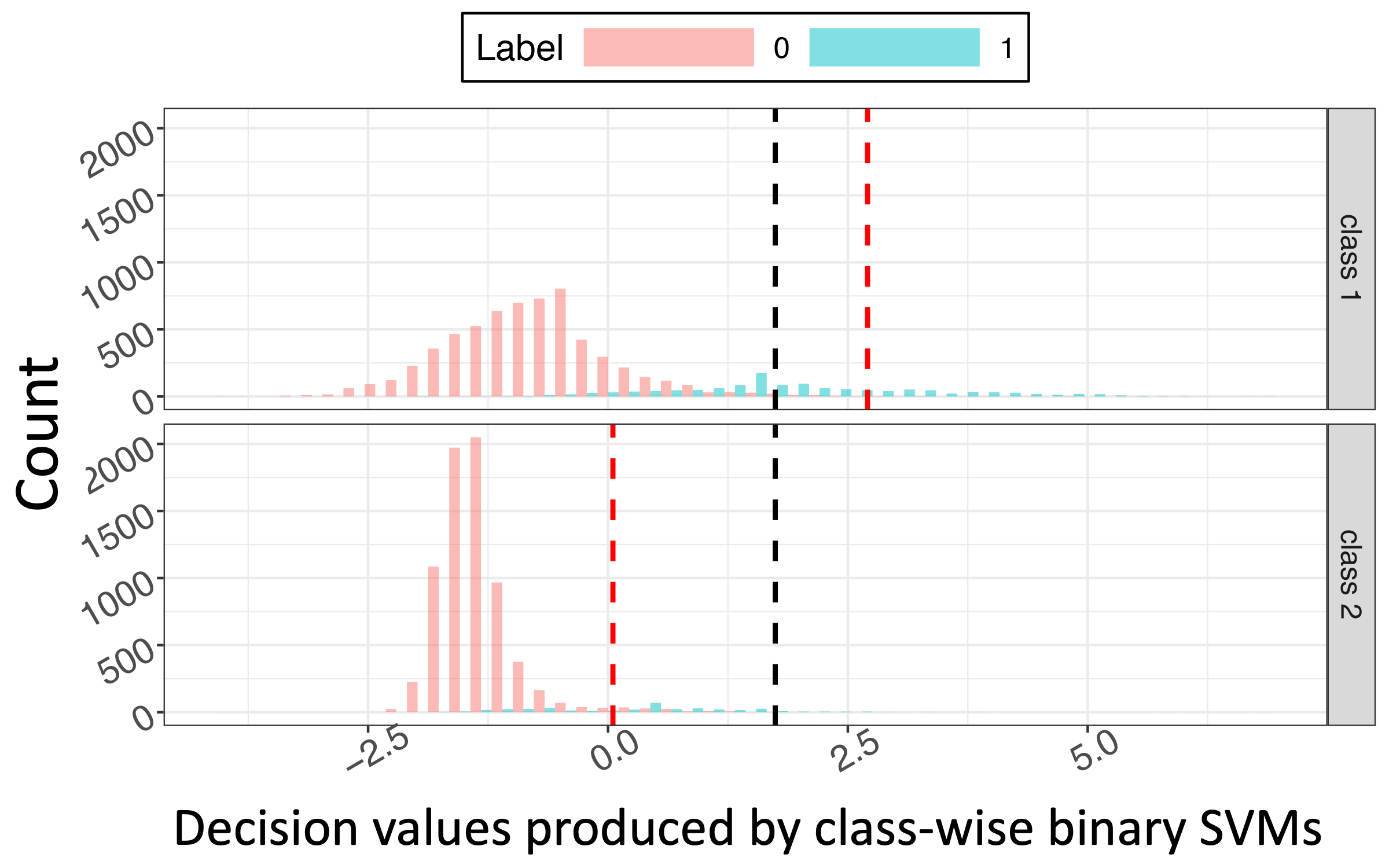
Figure S4: Distributions of the SVM (support vector machine) output values for two classes of the RCV1v2 data set (see Section 5.4 for details). The red vertical dashed lines indicate the respective $5\%$ quantiles of the two classes, and the black vertical dashed line indicates the $5\%$ quantile of the mix of the two classes. Making decisions on the mix of the output values of the two classes (e.g., using a decision rule to take the top $5\%$ samples) is likely to lead to a small power on the second class.

D.6 Training Strategy to Handle the Overfitting Issue for a Two-stage Method

We used the RCV1v2 data set to show how to handle the overfitting issue for our method. There are two training stages: 1) training classwise SVM to get first-stage classification scores, 2) training the LPR model using the SVM scores, and training learners to estimate $\operatorname*{\mathbb{P}}(Y_{i})$’s and $\operatorname*{\mathbb{P}}(Y_{i}|\operatorname*{\boldsymbol{\tilde{Y}}}_{pa(i)})$’s. A natural question that arises is whether we should conduct the two training stages on the same set of data or on different sets.

For a fair evaluation, we split the data set into three partitions: Partition I ($25\%$ of the samples), Partition II ($25\%$ of the samples), and Partition III ($50\%$ of the samples). First, we trained SVMs on partition I, and then predicted the classification scores on each partition (Figure S5a (a)). The distribution of the classification scores on Partition I differs far from those on Partition II and Partition III, while the latter two distributions are quite similar. This is reasonable since Partition I is the training data set, and Partition II & III are the testing data sets for the first stage. For the estimation of the LPR (and other quantities), there are two possible training strategies:

1. Train the model for the LPR on Partition I and then predict the LPR scores on Partition II & III.

2. Train the model for the LPR on Partition II and then predict the LPR scores on Partition III.

We suggest using the second strategy. To elaborate on this point, we investigate the predicted LPR scores for both strategies. As shown in Figure S5a (b), for the first strategy, the distributions of the estimated LPRs are mixed between the positive and the negative groups on Partition II & III, while the distributions are clearly separated on Partition I. This results from the fact that the distribution of the input SVM scores on Partition I is much different from that on Partition II & III. It leads to a bad generalization from the training data to the testing data. By contrast, this issue disappears for the second strategy because, in this situation, the input SVM scores have similar distributions on Partition II and III. As a result, the distributions of the estimated LPRs between two groups are well separated on both Partition II and III. Similar phenomena are observed for the estimation of $\operatorname*{\mathbb{P}}(Y_{i})$ and $\operatorname*{\mathbb{P}}(Y_{i}|\operatorname*{\boldsymbol{\tilde{Y}}}_{pa(i)})$.

(a) SVM scores.

Figure S5: Predicted SVM/LPR scores. (a) The SVM model was trained on Partition I, and predicted on all partitions. (b) The LPR models were respectively trained on Partition I then predicted on all partitions (left), and trained on Partition II then predicted on Partition II & III (right).

  

(b) LPR scores.

Remark S4

We point out that we trimmed the factor $1/\hat{\operatorname*{\mathbb{P}}}(Y_{i})$ since it can be quite unstable if $\hat{\operatorname*{\mathbb{P}}}(Y_{i})$ is close to $0$. This strategy has been commonly adopted in statistics and machine learning. The Iterated Probability Weights method in causal inference (Lee et al., 2011) and varieties of deep neural networks (Pascanu et al., 2013) use the clipping trick.

Appendix E Proofs of Theorems

Here, we give the detailed proofs of Theorem 3, Theorem 5, Theorem S1.

E.1 Proof of Theorem 3

We make the below assumptions for Theorem 3.

• $f_{0,k}$ and $f_{1,k}$ are continuous with $\zeta:=\max_{k=1,\ldots,K}\max\{\|f_{1,k}\|_{\infty},\|f_{0,k}\|_{\infty}\}<\infty$, where $\|\cdot\|_{\infty}$ is the infinity norm; $f_{1,k}$ and $f_{0,k}$ are the densities of $F_{1,k}$ and $F_{0,k}$ respectively, $k=1,\ldots,K$.

• The kernel function $K:\operatorname*{\mathbb{R}}\rightarrow[0,\infty)$ satisfies

  • $\int_{\operatorname*{\mathbb{R}}}K(u)du=1$.

  • $K$ is non-increasing.

  • There exists $\rho,C_{\rho},u_{0}>0$ such that for $|u|>u_{0}$, $K(|u|)\leq C_{\rho}\cdot\exp(-u^{\rho})$, i.e., $K$ has an exponential decays.

  These assumptions allow the popular kernels including Gaussian, Exponential, Silverman, uniform, triangular, tricube, Cosine, and Epanechnikov.

• The bandwidth for the kernel density estimator satisfies $h>(\log M)/M$. Particularly, we take $h_{n}=\left[(\log M)/{M}\right]^{1/3}$.

Proof  Note that we can write $LPR_{k}(s)=1-(1-\tau_{k})f_{0,k}(s)/{f_{k}(s)}$, where $s$ is a score and $\tau_{k}$ is the probability of $s$ being sampled from the alternative distribution $F_{1,k}$, and $f_{k}$ is the joint density of the null distribution and the alternative distribution. We can use Kernel density estimation to estimate $f_{0,k}$ and $f_{k}$.

Under Assumptions A1, A2 and A3, and by Theorem 1 of Jiang (2017), then with probability at least $1-1/M$, we have

$$\|\hat{f}_{0,k;h}-f_{0,k}\|_{\infty}\leq D_{1}\cdot h+D_{2}\frac{\log M}{M\cdot h},$$

where $\hat{f}_{0,k;h}$ is a kernel density estimator of $f_{0,k}$ with a band width $h$; $D_{1},D_{2}>0$ depend on $K$ and $\max_{k=1,\ldots,K}\|f_{0,k}\|_{\infty}$. When taking $h=\sqrt[3]{(\log M)/M}$, we have

$$\|\hat{f}_{0,k;h}-f_{0,k}\|_{\infty}\leq D_{3}\cdot\sqrt[3]{\frac{\log M}{M}}~{}~{}~{}~{}~{}\text{with probability }1-1/M,$$

where $D_{3}$ is a function of $D_{1}$ and $D_{2}$. Note that these results are uniform w.r.t $s$ and $k$. We have similar uniform convergence results for $\hat{f}_{k;h}$.

Furthermore, we use empirical estimators to estimate $\operatorname*{\mathbb{P}}(Y_{k}=1):=\tau_{k}$ and $\operatorname*{\mathbb{P}}(Y_{k}=1|\operatorname*{\boldsymbol{Y}}_{pa(k)})$. To be specific, $\hat{\tau}_{k}=\sum_{m=1}^{M}\operatorname*{\mathbb{I}}[Y_{k}^{(m)}=1]/M$. Since $\operatorname*{\mathbb{I}}$ is bounded, by Hoeffding’s bound, it is easy to see that

$$\operatorname*{\mathbb{P}}(|\hat{\tau}_{k}-\tau_{k}|\geq t)\leq\exp(-\frac{Mt^{2}}{2}).$$

Taking $t=\sqrt{2(\log M)/M}$, we have

$$|\hat{\tau}_{k}-\tau_{k}|\leq\sqrt{\frac{2\log M}{M}}~{}~{}~{}~{}~{}\text{with probability }1-1/M.$$

Similar results can be established for the empirical estimators of $\operatorname*{\mathbb{P}}(Y_{k}|\operatorname*{\boldsymbol{Y}}_{pa(k)})$. Note that these results are uniform for $k=1,\ldots,K$.

Finally, we use (4.1) to get the marginal $mLPR_{i}=\operatorname*{\mathbb{P}}(Y_{i}=1|S_{1},\ldots,S_{n})$. Since different samples are independent, we just need to consider $\operatorname*{\mathbb{P}}(Y_{1},\ldots,Y_{K}|S_{1},\ldots,S_{K})$. Putting the above results for $LPR_{k}$ and $\operatorname*{\mathbb{P}}(Y_{k})$, $\operatorname*{\mathbb{P}}(Y_{k}|\operatorname*{\boldsymbol{Y}}_{pa(k)})$ together, the estimated potential of the $k$-th class satisfies

$$|\hat{\psi}_{k}-\psi_{k}|\leq D_{4}\cdot\sqrt[3]{\frac{\log M}{M}}~{}~{}~{}~{}~{}\text{with probability }1-2/M,$$

where $D_{4}$ is some positive constant that depends on $K$ and the upper bound of $\zeta$, which is universal for all $i=1,\ldots,n$, and

$$\psi(\boldsymbol{Y}_{pa(k)},Y_{k}):=LPR_{k}\cdot\frac{\operatorname*{\mathbb{P}}(Y_{k}|\operatorname*{\boldsymbol{Y}}_{pa(k)})}{\operatorname*{\mathbb{P}}(Y_{k})},\quad\hat{\psi}(\boldsymbol{Y}_{pa(k)},Y_{k})=\widehat{LPR}_{k}\cdot\frac{\widehat{\operatorname*{\mathbb{P}}}(Y_{k}|\operatorname*{\boldsymbol{Y}}_{pa(k)})}{\widehat{\operatorname*{\mathbb{P}}}(Y_{k})}.$$

Using the elimination trick (Wainwright and Jordan, 2008), and noting that there are at most $2^{d_{k}}$ summations when eliminating the $k$-th class with degree $d_{k}$ in $\operatorname*{\mathcal{G}}$, it follows that

$$|\widehat{mLPR}_{i}-mLPR_{i}|\leq C_{2}\sum_{k=1}^{K}2^{d_{k}}\cdot\left(\frac{\log M}{M}\right)^{1/3}\text{ with probability }(1-2/M)^{\sum_{k=1}^{K}2^{d_{k}}},$$

where $C_{2}$ is some positive constant that depends on $K$ and the upper bound of $\zeta$; it is universal for all $i=1,\ldots,n$. By using the bound $\sum_{k=1}^{K}2^{d_{k}}\leq K\cdot 2^{d}$, where $d=\max_{k=1,\ldots,K}d_{k}$, and employing the inequality $(1-x)^{r}\geq 1-rx$ for positive $x$ and $r$, we complete the proof.

 

E.2 Proof of Theorem 5

Proof  The simplest case is a graph with only one chain, and the theorem obviously holds for this case. Next, suppose there are two chain branches, $X_{(1)}\rightarrow\ldots\rightarrow X_{(m)}$ and $Y_{(1)}\rightarrow\ldots\rightarrow Y_{(m^{\prime})}$, both of which share the same parent node in $\operatorname*{\mathcal{P}}_{2}$. Directly merging these two chain branches by Algorithm 2 yields an ordering denoted as $o_{XY}$. Now given an arbitrary ordering $o_{A}$ of all the $n$ nodes in the entire graph, which respects the tree hierarchy. Denote by $p_{1}$ the first position of the nodes among $X_{(i)}^{\prime}s$ and $Y_{(j)}^{\prime}s$ within $o_{A}$, and denote all the nodes, other than $X_{(i)}^{\prime}s$ and $Y_{(j)}^{\prime}s$ and located after the $p_{1}$ position, by $W_{(1)},\ldots,W_{(n^{\prime})}$ (the position of $W_{(l)}$ is ahead of that of $W_{(l^{\prime})}$ in $o_{A}$ if $l<l^{\prime}$). We want to show that

Lemma S5

There exists a topological ordering $o_{A^{\prime}}$ of $\operatorname*{\mathcal{G}}$ that is at least as good as $o_{A}$, in terms of CATCH, such that $(\star)$ Node $B$ is located ahead of Node $C$ in $o_{A}$ if it is the case in $o_{XY}$, where $B$, $C$ are two distinct nodes among $X_{(i)}^{\prime}s$ and $Y_{(i)}^{\prime}s$.

Lemma S5 implies that in order to figure out the optimal ordering of the original tree structure, it boils down to replacing the two branches $X_{(1)},\ldots,X_{(m)}$ and $Y_{(1)},\ldots,Y_{(m^{\prime})}$ by a single chain characterized by $o_{XY}$ and seeking the optimal ordering of the new structure. The ordering $o_{A^{\prime}}$ mentioned above can be constructed easily with two constraints:

• Fixing the nodes located ahead of the position $p_{1}$ as well as their ordering as in $o_{A}$.

• The position of $W_{(l)}$ is ahead of $W_{(l^{\prime})}$ if $l<l^{\prime}$, as in $o_{A}$.

The first constraint is straightforward, and the second constraint can be satisfied by applying Algorithm 2 to $X_{(1)},\ldots,X_{(m)}$, $Y_{(1)},\ldots,Y_{m^{\prime}}$ and $W_{(1)},\ldots,W_{(n^{\prime})}$. Here, we take $W_{(1)},\ldots,W_{(n^{\prime})}$ as a chain, regardless of their original structure. Without loss of generality, we assume the first chain branch with the maximal mean score value figured out by Algorithm 2 is $X_{(1)},\ldots,X_{(t)}$, $t\leq m$ (we can skip the case that Algorithm 2 first picks a part of $W_{(l)}$’s since it does not affect ($\star$)). In order to prove Lemma S5, it is reduced to showing that

Lemma S6

Conditional on (i) and (ii), the ordering with the maximal CATCH puts $X_{(1)},\ldots,X_{(t)}$ at the position $p_{1},\ldots,p_{1}+t-1$ respectively.

The detailed proof of Lemma S6 is deferred to Appendix E.3. Note that $X_{(1)},\ldots,X_{(t)}$ must be located in the first place in the ordering $o_{XY}$. Therefore, by applying Lemma S6 in an inductive way (exclude $X_{(1)},\ldots,X_{(t)}$ and apply the same argument on the remaining nodes), we can conclude the constructed $o_{A^{\prime}}$ is at least as good as $o_{A}$ and satisfies $(\star)$. Here, we need to clarify the point that putting $X_{(1)},\ldots,X_{(t)}$ in such place does not violate the tree hierarchy since $X_{(i)}^{\prime}s$ and $Y_{(j)}^{\prime}s$ are the children chains of the same node, and none of $W_{(l)}^{\prime}s$ can be an ancestor of $X_{(i)}^{\prime}s$ or $Y_{(j)}^{\prime}s$ (otherwise $o_{A}$ is not a valid ordering). Thus the proof is completed.  

E.3 Proof of Lemma S6

Proof 
Let $a$ denote the mean of these $t$ values, i.e., $a:=\sum_{k=1}^{t}X_{(k)}$. For the sake of simplicity, we further assume $p_{1}=1$ and simply denote by $Z_{(1)},\ldots,Z_{(n-t)}$ the combination of $X_{(t+1)},\ldots,X_{(m)}$, $Y_{(j)}^{\prime}s$ and $W_{(l)}^{\prime}s$. Let the ordering $o_{A}$ be as follows:

$$\begin{array}[]{ccccccccccc}Z_{(1)}&\ldots&Z_{(i_{1}-1)}&X_{(1)}&Z_{(i_{1})}&\ldots&Z_{(i_{t}-t)}&X_{(t)}&Z_{(i_{t}-t+1)}&\ldots&Z_{(n-t)}\\ 1&\ldots&i_{1}-1&i_{1}&i_{1}+1&\ldots&i_{t}-1&i_{t}&i_{t}+1&\ldots&n\end{array}$$

where $i_{c}$ is the position of $X_{(c)}$, $c=1,\ldots,t$. Note that $i_{c+1}\geq i_{c}+1$. Denote by $o_{A_{1}^{\prime}}$ the ordering of $(X_{(1)},\ldots,X_{(t)})+o_{A}/(X_{(1)},\ldots,X_{(t)})$, that is, move $(X_{(1)},\ldots,X_{(t)})$ to the head of $o_{A}$. The difference in the value of the objective function (OF) between $o_{A^{\prime}_{1}}$ and $o_{A}$ can be written as follows:

$$\text{OF of }o_{A^{\prime}_{1}}= \sum_{i=1}^{t}(n-i+1)X_{(i)}+\sum_{j=1}^{n-t}(n-t-j+1)Z_{(j)},$$

$$\text{OF of }o_{A}= (n-i_{1}+1)X_{(1)}+\ldots+(n-i_{t}+1)X_{(t)}$$

$$+\sum_{j=1}^{i_{1}-1}(n-j+1)Z_{(j)}+\ldots+\sum_{j=i_{t}-t+1}^{n-t}(n-(j+t)+1)Z_{(j)}.$$

$$\text{OF of }o_{A^{\prime}_{1}}-\text{OF of }o_{A}=\left[(i_{1}-1)X_{(1)}-\sum_{k=1}^{i_{1}-1}Z_{(k)}\right]+\ldots+\left[(i_{t}-t)X_{(t)}-\sum_{k=1}^{i_{t}-t}Z_{(k)}\right]$$

$$=(i_{1}-1)\left[X_{(1)}-\frac{1}{i_{1}-1}\sum_{k=1}^{i_{1}-1}Z_{(k)}\right]+\ldots+(i_{t}-t)\left[X_{(t)}-\frac{1}{i_{t}-t}\sum_{k=1}^{i_{t}-t}Z_{(k)}\right]$$

$$=(i_{1}-1)\left[\left(X_{(1)}-a\right)+\left(a-\frac{1}{i_{1}-1}\sum_{k=1}^{i_{1}-1}Z_{(k)}\right)\right]+\ldots$$

$$\quad\quad\quad\quad+(i_{t}-t)\left[\left(X_{(t)}-a\right)+\left(a-\frac{1}{i_{t}-t}\sum_{k=1}^{i_{t}-t}Z_{(k)}\right)\right]$$

$$=\left[(i_{1}-1)\left(X_{(1)}-a\right)+\ldots+(i_{t}-t)\left(X_{(t)}-a\right)\right]$$

$$\quad\quad\quad\quad+\left[(i_{1}-1)\left(a-\frac{1}{i_{1}-1}\sum_{k=1}^{i_{1}-1}Z_{(k)}\right)+(i_{t}-t)\left(a-\frac{1}{i_{t}-t}\sum_{k=1}^{i_{t}-t}Z_{(k)}\right)\right].$$

It remains to prove both the first term and the second term on the right side are non-negative:

• The first term. We can rewrite the sum $(i_{1}-1)\left(X_{(1)}-a\right)+\ldots+(i_{t}-t)\left(X_{(t)}-a\right)$ as follows

  $$(i_{1}-1)\sum_{k=1}^{t}(X_{(k)}-a)\ +\ (i_{2}-i_{1}-1)\sum_{k=2}^{t}\left(X_{(k)}-a\right)+\ldots+(i_{t}-i_{t-1}-1)(X_{(t)}-a).$$

  The first sum $\sum_{k=1}^{t}(X_{(k)}-a)=0$ since $a$ is the mean. The other sums being nonnegative follows from the fact that $a$ must be at least as high as the lower means in the chain, i.e. $a\geq\sum_{k=1}^{c}X_{(k)}/c$ where $1\leq c\leq t$. In detail, we know that

  $$X_{(c+1)}+\ldots+X_{(t)} =ta-[X_{(1)}+\ldots+X_{(c)}],\quad 1\leq c\leq t-1$$

  $$\geq ta-ca=(t-c)a.$$

  $$\text{So }(X_{(c+1)}-a)+\ldots+(X_{(t)}-a) \geq 0.$$

  Therefore, each sum

  $$\sum_{k=c}^{t}\left(X_{(k)}-a\right)\geq 0,~{}~{}~{}c=1,\ldots,t.$$ (E.1)

  It is clear that the expression

  $$(i_{1}-1)\sum_{k=1}^{t}(X_{(k)}-a)\ +\ (i_{2}-i_{1}-1)\sum_{k=2}^{t}\left(X_{(k)}-a\right)+\ldots+(i_{t}-i_{t-1}-1)(X_{(t)}-a)$$

  is exactly zero only when each $X_{(c)}=a$.

• The second term. We claim that each term in the expression

  $$\left[(i_{1}-1)\left(a-\frac{1}{i_{1}-1}\sum_{k=1}^{i_{1}-1}Z_{(k)}\right)+(i_{t}-t)\left(a-\frac{1}{i_{t}-t}\sum_{k=1}^{i_{t}-t}Z_{(k)}\right)\right]$$

  must be nonnegative, and equality holds only if there is a tie. To see this, we notice that $\sum_{k=1}^{i_{c}-c}Z_{(k)}$ can be separated as three sums: $\sum_{k=t+1}^{t_{X}}X_{(k)}$, $\sum_{k=1}^{t_{Y}}Y_{(k)}$ and $\sum_{k=1}^{t_{W}}W_{(k)}$, where $t_{X}\leq m$, $t_{Y}\leq m^{\prime}$, $t_{W}\leq n^{\prime}$ and $c=t_{X}-t+t_{Y}+t_{W}$. In terms of the procedure of Algorithm 2, it follows that

  $$\sum_{k=1}^{t_{Y}}Y_{(k)}\leq t_{Y}\cdot a~{}~{}~{}~{}~{}\text{and}~{}~{}~{}~{}~{}\sum_{k=1}^{t_{W}}W_{(k)}\leq t_{W}\cdot a.$$

  For the same reason, $\sum_{k=t+1}^{t_{X}}X_{(k)}\leq(t_{X}-t)a$, otherwise we have $\sum_{k=1}^{t_{X}}X_{(k)}/{t_{X}}>a$ and it violates the condition that $a$ is the mean of the chain branch with the highest mean score . So we have

  $$\frac{1}{i_{c}-c}\sum_{k=1}^{i_{c}-c}Z_{(k)}=\frac{1}{i_{c}-c}[\sum_{k=t+1}^{t_{X}}X_{(k)}+\sum_{k=1}^{t_{Y}}Y_{(k)}+\sum_{k=1}^{t_{W}}W_{(k)}]\leq a.$$

 

E.4 Proof of Theorem S1

Proof  To establish the bridge between HierRank (Algorithm 1) and Algorithm S2, we start from a simple case, i.e., a tree consisting of multiple chains with the same root (the root is in $\operatorname*{\mathcal{P}}_{2}$). Specifically, denote by $R$ the root and these children chain by $C_{s}:=\{X_{1}^{(s)},\ldots,X_{k_{s}}^{(s)}\}$, $s=1,\dots,\nu$, where $\nu$ is the number of chains, and $k_{s}$ is the length of the $s_{th}$ chain. Without loss of generality, suppose $T_{1}:=C_{1}(h_{1})=\{X_{1}^{(1)},\dots,X_{h_{1}}^{(1)}\}$ is the first supernode that has been condensed to $R$, if $R$ has not been taken off, or the first to be taken off after $R$. We claim that

Lemma S7

When merging $C_{1},\ldots,C_{\nu}$, Algorithm 2 puts $T_{1}$ in the first place.

To show Lemma S7, we only need to show $\sum_{k\in C_{1}(h_{1})}S_{k}/{h_{1}}\geq\sum_{k\in C_{s}(h)}S_{k}/h$, $\forall~{}h\in\{1,\ldots,k_{s}\},s\in\{1,\ldots,\nu\}$. The detailed proof is deferred to Appendix E.5. Inductively, it implies that the ordering given by Algorithm S2 on such simple case is the same as HierRank. Furthermore, any complicated structure boils down to the above simple case, since we can inductively merge the sub-chains starting from a root in $\operatorname*{\mathcal{P}}_{2}$ using Algorithm 2. This completes the proof showing that the results of HierRank and Algorithm S2 are the same.  

E.5 Proof of Lemma S7

Proof  We show the proof in three steps:

• Along the chain $C_{1}$, all the sub-chains starting from $X_{1}^{(1)}$ with larger length than $T_{1}$ have at most as high mean score as $T_{1}$, that is, $\bar{\ell}(1,h)\leq\bar{\ell}(1,h_{1})$, $\forall h_{1}<h\leq k_{1}$. In terms of the procedure of Algorithm S2, all the mean score values in the supernodes following $T_{1}$ is no higher than $\bar{\ell}(1,h_{1})$.

• Along the chain $C_{1}$, all the sub-chains starting from $X_{1}^{(1)}$ with smaller length than $T_{1}$ have at most as high mean score as $T_{1}$, that is, $\bar{\ell}(1,h)\leq\bar{\ell}(1,h_{1})$, $\forall 1\leq h<h_{1}$. Otherwise, suppose $h_{1}^{\prime}<h_{1}$ s.t. $X_{1}^{(1)},\ldots,X^{(1)}_{h_{1}^{\prime}}$ is the sub-chain with the highest mean score and $\bar{\ell}(1,h_{1}^{\prime})>\bar{\ell}(1,h_{1})$. By Eq. (E.1), we know that $\sum_{i=c}^{h_{1}^{\prime}}(X_{i}^{(1)}-\bar{\ell}(1,h_{1}^{\prime}))\geq 0$, $c=1,\ldots,h_{1}^{\prime}$. So to make any supernode right behind the one ending with $X_{h_{1}^{\prime}}^{(1)}$ merged with its former supernode, the mean score value of this supernode must be at least $\bar{\ell}(1,h_{1}^{\prime})$. Thus, we can inductively conclude that $\bar{\ell}(1,h_{1})\geq\bar{\ell}(1,h_{1}^{\prime})$, which is a contradiction.

• $\bar{\ell}(s,h)\leq\bar{\ell}(1,h_{1})$, $\forall h\in\{1,\ldots,k_{s}\},s\in\{1,\ldots,\nu\}$. Otherwise, without loss of generality, suppose $X_{1}^{(2)},\ldots,X^{(2)}_{h_{2}}$ is the sub-chain with the highest mean score and $\bar{\ell}(2,h_{2})>\bar{\ell}(1,h_{1})$. By Eq. (E.1), any super node ending with $X_{h_{2}}^{(2)}$ has an mean score of at least $\bar{\ell}(2,h_{2})$. Then it contradicts with the assumption that $T_{1}$ is the first supernode that will be merged with $R$, if $R$ has not been taken off, or by the time $T_{1}$ is taken off.

References

- Alves et al. (2010) R. T. Alves, M. Delgado, and A. A. Freitas. Knowledge discovery with artificial immune systems for hierarchical multi-label classification of protein functions. In IEEE International Conference on Fuzzy Systems, pages 1–8, 2010.
- Ananpiriyakul et al. (2014) T. Ananpiriyakul, P. Poomsirivilai, and P. Vateekul. Label correction strategy on hierarchical multi-label classification. In International Workshop on Machine Learning and Data Mining in Pattern Recognition, pages 213–227, 2014.
- Baraniuk (1999) R. G. Baraniuk. Optimal tree approximation with wavelets. In Wavelet Applications in Signal and Image Processing VII, volume 3813, pages 196–208, 1999.
- Baraniuk and Jones (1994) R. G. Baraniuk and D. L. Jones. A signal-dependent time-frequency representation: Fast algorithm for optimal kernel design. IEEE Transactions on Signal Processing, 42(1):134–146, 1994.
- Baraniuk et al. (2010) R. G. Baraniuk, V. Cevher, M. F. Duarte, and C. Hegde. Model-based compressive sensing. IEEE Transactions on Information Theory, 56(4):1982–2001, 2010.
- Barutcuoglu et al. (2006) Z. Barutcuoglu, R. E. Schapire, and O. G. Troyanskaya. Hierarchical multi-label prediction of gene function. Bioinformatics, 22(7):830–836, 2006.
- Bi and Kwok (2011) W. Bi and J. T. Kwok. Multi-label classification on tree-and dag-structured hierarchies. In International Conference on Machine Learning, pages 17–24, 2011.
- Bi and Kwok (2015) W. Bi and J. T. Kwok. Bayes-optimal hierarchical multilabel classification. IEEE Transactions on Knowledge and Data Engineering, 27(11):2907–2918, 2015.
- Blockeel et al. (2002) H. Blockeel, M. Bruynooghe, S. Dzeroski, J. Ramon, and J. Struyf. Hierarchical multi-classification. In ACM SIGKDD 2002 Workshop on Multi-relational Data Mining, pages 21–35, 2002.
- Blockeel et al. (2006) H. Blockeel, L. Schietgat, J. Struyf, S. Džeroski, and A. Clare. Decision trees for hierarchical multilabel classification: A case study in functional genomics. In European Conference on Principles of Data Mining and Knowledge Discovery, pages 18–29, 2006.
- Chen et al. (2019) H. Chen, S. Miao, D. Xu, G. D. Hager, and A. P. Harrison. Deep hierarchical multi-label classification of chest x-ray images. In International Conference on Medical Imaging with Deep Learning, pages 109–120, 2019.
- Davis and Goadrich (2006) J. Davis and M. Goadrich. The relationship between precision-recall and roc curves. In International Conference on Machine Learning, pages 233–240, 2006.
- DeCoro et al. (2007) C. DeCoro, Z. Barutcuoglu, and R. Fiebrink. Bayesian aggregation for hierarchical genre classification. International Society for Music Information Retrieval, pages 77–80, 2007.
- Dimitrovski et al. (2011) I. Dimitrovski, D. Kocev, S. Loskovska, and S. Džeroski. Hierarchical annotation of medical images. Pattern Recognition, 44(10):2436–2449, 2011.
- Efron (2012) B. Efron. Large-scale Inference: Empirical Bayes Methods for Estimation, Testing, and Prediction, volume 1. Cambridge University Press, 2012.
- Feng et al. (2017) S. Feng, P. Fu, and W. Zheng. A hierarchical multi-label classification algorithm for gene function prediction. Algorithms, 10(4):138, 2017.
- Gupta et al. (2016) V. Gupta, H. Karnick, A. Bansal, and P. Jhala. Product classification in e-commerce using distributional semantics. In International Conference on Computational Linguistics: Technical Papers, pages 536––546, 2016.
- Hand (2009) D. J. Hand. Measuring classifier performance: a coherent alternative to the area under the roc curve. Machine learning, 77(1):103–123, 2009.
- Herskovic et al. (2007) J. R. Herskovic, M. S. Iyengar, and E. V. Bernstam. Using hit curves to compare search algorithm performance. Journal of Biomedical Informatics, 40(2):93–99, 2007.
- Ho et al. (2018) C. Ho, Y. Ye, C.-R. Jiang, W. T. Lee, and H. Huang. Hierlpr: Decision making in hierarchical multi-label classification with local precision rates. arXiv preprint arXiv:1810.07954, 2018.
- Huang et al. (2010) H. Huang, C.-C. Liu, and X. J. Zhou. Bayesian approach to transforming public gene expression repositories into disease diagnosis databases. Proceedings of the National Academy of Sciences, 107(15):6823–6828, 2010.
- Jiang et al. (2014) C.-R. Jiang, C.-C. Liu, X. J. Zhou, and H. Huang. Optimal ranking in multi-label classification using local precision rates. Statistica Sinica, 24(4):1547–1570, 2014.
- Jiang (2017) H. Jiang. Uniform convergence rates for kernel density estimation. In International Conference on Machine Learning, pages 1694–1703, 2017.
- Kahanda and Ben-Hur (2017) I. Kahanda and A. Ben-Hur. Gostruct 2.0: Automated protein function prediction for annotated proteins. In ACM International Conference on Bioinformatics, Computational Biology, and Health Informatics, pages 60–66, 2017.
- Lee et al. (2011) B. K. Lee, J. Lessler, and E. A. Stuart. Weight trimming and propensity score weighting. PLOS One, 6(3), 2011.
- Lee (2013) W. T. Lee. Bayesian Analysis in Problems with High Dimensional Data and Complex Dependence Structure. PhD thesis, University of California, Berkeley, 2013.
- Lewis et al. (2004) D. D. Lewis, Y. Yang, T. G. Rose, and F. Li. Rcv1: A new benchmark collection for text categorization research. Journal of Machine Learning Research, 5(Apr):361–397, 2004.
- Makrodimitris et al. (2019) S. Makrodimitris, R. C. van Ham, and M. J. Reinders. Improving protein function prediction using protein sequence and go-term similarities. Bioinformatics, 35(7):1116–1124, 2019.
- Nakano et al. (2019) F. K. Nakano, M. Lietaert, and C. Vens. Machine learning for discovering missing or wrong protein function annotations. BMC bioinformatics, 20(1):1–32, 2019.
- Pascanu et al. (2013) R. Pascanu, T. Mikolov, and Y. Bengio. On the difficulty of training recurrent neural networks. In International Conference on Machine Learning, pages 1310–1318, 2013.
- Pham et al. (2021) H. H. Pham, T. T. Le, D. Q. Tran, D. T. Ngo, and H. Q. Nguyen. Interpreting chest x-rays via cnns that exploit hierarchical disease dependencies and uncertainty labels. Neurocomputing, 437:186–194, 2021.
- Ploner et al. (2006) A. Ploner, S. Calza, A. Gusnanto, and Y. Pawitan. Multidimensional local false discovery rate for microarray studies. Bioinformatics, 22(5):556–565, 2006.
- Salama and El-Gohary (2016) D. M. Salama and N. M. El-Gohary. Semantic text classification for supporting automated compliance checking in construction. Journal of Computing in Civil Engineering, 30(1):04014106, 2016.
- Silla and Freitas (2011) C. N. Silla and A. A. Freitas. A survey of hierarchical classification across different application domains. Data Mining and Knowledge Discovery, 22(1-2):31–72, 2011.
- Triguero and Vens (2016) I. Triguero and C. Vens. Labelling strategies for hierarchical multi-label classification techniques. Pattern Recognition, 56:170–183, 2016.
- Valentini (2011) G. Valentini. True path rule hierarchical ensembles for genome-wide gene function prediction. IEEE/ACM Transactions on Computational Biology and Bioinformatics, 8(3):832–847, 2011.
- Vens et al. (2008) C. Vens, J. Struyf, L. Schietgat, S. Džeroski, and H. Blockeel. Decision trees for hierarchical multi-label classification. Machine Learning, 73(2):185–214, 2008.
- Wainwright and Jordan (2008) M. J. Wainwright and M. I. Jordan. Graphical Models, Exponential Families, and Variational Inference. Germany: Now Publishers, 2008.
- Yang and Koyejo (2020) F. Yang and S. Koyejo. On the consistency of top-k surrogate losses. In International Conference on Machine Learning, pages 10727–10735, 2020.
- Yang et al. (2018) L. Yang, A. M. MacEachren, P. Mitra, and T. Onorati. Visually-enabled active deep learning for (geo) text and image classification: a review. ISPRS International Journal of Geo-Information, 7(2):65, 2018.
- Zeng et al. (2017) C. Zeng, W. Zhou, T. Li, L. Shwartz, and G. Y. Grabarnik. Knowledge guided hierarchical multi-label classification over ticket data. IEEE Transactions on Network and Service Management, 14(2):246–260, 2017.
- Zhang and Zhou (2013) M.-L. Zhang and Z.-H. Zhou. A review on multi-label learning algorithms. IEEE Transactions on Knowledge and Data Engineering, 26(8):1819–1837, 2013.