Multi–Species Thermalization Cascade of Energetic Particles in the Early Universe

Abstract

Heavy long–lived particles are abundant in BSM physics and will, under generic circumstances, get to dominate the energy density of the universe. The resulting matter dominated era has to end before the onset of Big Bang Nucleosynthesis through the decay of the heavy matter component of mass $M$ into a thermal bath of temperature $T$. The process of thermalization primarily involves near–collinear splittings of energetic particles into two particles with lower energy. The correct treatment of these processes requires the inclusion of coherence effects which suppress the splitting rate. We write down and numerically solve the resulting coupled Boltzmann equations including all gauge bosons and fermions of the Standard Model (SM). We then comment on the dependence of the nonthermal spectra on the ratio $M/T$, as well as on the matter decay rate and branching ratios into various SM particles.

1 Introduction

Top–down approaches to the history of the universe, as in UV complete theories of inflation, likely include some scalar field, e.g. the inflaton itself or an additional “modulus” field, that is initially displaced from its low energy minimum and later oscillates around this minimum; if the potential around the minimum can be described by a quadratic function this corresponds to a non–relativistic (matter) component [1, 2, 3, 4]. Given enough time, a matter component will grow to dominate the energy density of the universe because of its different equation of state compared to radiation [1]. On the other hand, we know from cosmological observations that the universe was indeed radiation dominated during Big Bang Nucleosynthesis (BBN) [5, 6, 7]. Hence any dominant matter content must have decayed, and the decay products thermalized into the thermal bath, before the onset of BBN at a temperature of about $3\text{\,}\mathrm{MeV}$.

An early epoch of matter domination affects the density of (semi–)stable relics in several ways. First of all, the entropy released by the decay of the heavy matter particles dilutes any possible pre–existing relic density of decoupled species [1, 8, 9]. Moreover, for a given temperature $T$ the Hubble expansion rate is higher than in a radiation–dominated era, which increases the thermal freeze–out temperature. Finally, relics can be produced non–thermally, either directly in the decay of the heavy particles, or in collisions of energetic daughter particles with the thermal background or with each other [10, 11, 12, 13, 14, 15, 16, 17, 18, 19, 20, 21, 22, 24, 23, 25, 26, 27, 28, 29, 30, 31]. It has also been suggested that the energetic decay products can produce the baryon asymmetry via lepton– or baryon number violating scattering reactions on the thermal plasma [32, 33]. A quantitative treatment of production rates due to the scattering of highly energetic decay products requires a good understanding of their number density and energy distributions. In particular, knowledge of the chemical composition of the thermalizing decay products is crucial.

The process of thermalization leads to the growth of the number density of high energy particles while simultaneously reducing the average energy of the out of equilibrium states. In cosmology, it is well established [34, 12, 35, 18, 30, 36] that the process of thermalization for gauge interacting particles is driven by $2\rightarrow 3$ processes; in leading log approximation, these can be described as quasi–elastic $2\rightarrow 2$ reactions followed by a splitting process, with the parent high energy particle breaking up to two lower energy, nearly collinear daughter particles. As first pointed out in [35], the high collinearity of the daughter states calls for the inclusion of coherent multiple scatterings in the plasma, known as the Landau–Pomeranchuk–Migdal (LPM) effect [37, 38, 39]. Destructive interference between these interactions of the parent and daughter particles with the plasma leads to a parametrically suppressed splitting rate.

The process of energy loss of energetic gauge interacting particles in the presence of a thermal background has also been extensively studied in the context of Heavy Ion Collisions (HIC), and the physics of the resulting Quark-Gluon Plasma (QGP) [40, 41, 42, 43, 44]. Here the thermalization procedure evolves the initial spectrum of energetic partons traveling mostly along the beam directions towards a thermal distribution of quarks and gluons. Since color exchange is the dominant interaction in the QGP, most studies focus on colored matter; however, the emission of photons from the QGP and from electromagnetic plasmas have also been studied using the same machinery, as the photon spectrum serves as a probe of the QGP [45, 46, 47].

Although potentially on a very different energy scale, the physics of thermalization following matter decay is expected to be realized via the very same mechanisms as in the case of quark gluon plasmas resulting from HIC experiments [48]. In recent studies in the context of thermalization in cosmology [18, 30], analytical approximations to the resulting spectrum of thermalizing particles of a single species have been obtained. In [36], a more accurate numerical approach has been used to find this spectrum. Since the exchange and emission of non–Abelian gauge bosons is crucial in the thermalization, this approach is adequate for the description of pure Yang–Mills theories. Here the single species is a non–Abelian gauge boson and the LPM effect can be described by a single power law suppression. We will refer to such a treatment as the pure gauge treatment.

A pure gauge approximation is motivated by the fact that gauge boson emissions in a plasma are typically favored both by larger $\mathcal{O}\left({1}\right)$ group factors and by soft gauge boson emission enhancements, and in some cases by statistical enhancement and blocking factors [49]. In fact, the dominance of the $SU(3)_{C}$ interactions means that irrespective of the initial decay products, the energy density of the plasma can be expected to flow towards the colored sector and in particular to gluons, so that eventually a pure gluon plasma is a better approximation than that of $SU(2)$ gauge bosons. The single species approximation, however, does not answer the question of how quickly the chemical composition of the plasma flows towards the colored QCD sector, nor is it capable of estimating other subdominant contributions to the total out of equilibrium number density. Note that the primary matter decay products need not carry color. Moreover, many scattering reactions of interest may require particles other than gluons in the initial state. In these cases the spectra of other particles (than gluons) become particularly important.

In this study, we extend previous works by including all non–scalar species of the standard model in the thermalization cascade of energetic particles. This requires including the correct form for different vacuum splitting kernels, as well as the variations in the LPM suppression factor corresponding to the different Abelian and non–Abelian interactions of the charged particles involved in the splitting process. We also systematically consider different parent particles. We find that for sufficiently large ratios of the energy of the parent particle to the ambient temperature the spectrum of non–thermal particles will indeed eventually be dominated by gluons; however, for color singlet parent particles this will happen only at energies two to three orders of magnitude below that of the original particle. We also observe that the relative abundances of different species can vary by orders of magnitude, starkly different from the case of chemical equilibrium.

The remainder of this paper is organized as follows: in sec. 2 we review the framework of thermalization via collinear splitting processes including the LPM effect. Section 3 includes a formulation of the Boltzmann equations governing the number density of the various species. Numerical results are presented in sec. 4, whereas sec. 5 briefly sketches how to compute the production of massive particles in annihilation reactions involving one particle from the thermal bath and one particle from the non–thermal spectrum, followed by a summary and some concluding remarks in sec. 6.

2 Thermalization via splitting cascades

The process of thermalization of energetic decay products in cosmology involves an energetic particle losing energy by successive splittings to many lower energy particles; eventually, it injects energy into the thermal plasma. For parent particles charged under the gauge group of the Standard Model (SM), the underlying physics is similar to that of thermalization in heavy ion collisions. We will therefore use the results and conventions from this field. We will, however, only be interested in scenarios where an isotropic thermal plasma is already in place. We will first introduce the basic processes involved in the splitting cascade and the physics of the LPM suppression, before presenting the equations used to calculate the relevant rates.

Assuming the existence of a thermal bath of temperature $T$, we will be focusing on the thermalization of energetic parent particles of species $s$ and energy $E\approx p\gg T$ via interactions with the bath. It has been noted that the large energy suppresses the cross section for $2\rightarrow 2$ interactions except for $t-$channel forward scattering via exchange of a massless gauge boson [34]. The forward scattering cross section in vacuum is infrared (IR) divergent; this divergence is regulated by the thermal mass

$$m^{\scriptscriptstyle\rm th}_{G}\left({T}\right)\approx g_{G}T\,,$$ (2.1)

where $G\in\left\{C=SU(3)_{C},W=SU(2)_{L},Y=U(1)_{Y}\right\}$ denotes the dominant gauge group in the scattering process. Figure 1 shows schematically such an elastic process, with time flowing from left to right and the cross denoting a coupling to a particle in the thermal bath.

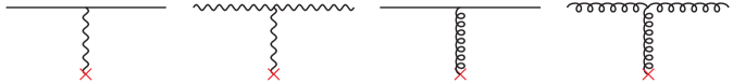
Figure 1: Elastic scattering processes of an energetic particle on the thermal bath mediated by a gauge boson; the former is denoted by the line on top while the the latter is represented by the cross at the bottom. The intermediate gauge boson should be considered as having acquired the thermal mass (2.1).

The crucial point is that strict forward scattering does not reduce the energy of the parent particle at all. In the presence of a thermal bath most elastic scattering reactions will have $|t|\sim\left(m^{\scriptscriptstyle\rm th}_{G}\right)^{2}$, and hence typical momentum exchange

$$\delta k^{\scriptscriptstyle\rm el}_{G}=m^{\scriptscriptstyle\rm th}_{G}\,.$$ (2.2)

The rate for these reactions is given by

$$\Gamma_{\scriptscriptstyle\rm el}^{s}\approx\tilde{g}_{*}^{s}\alpha_{G}T\,\equiv 1/t_{\scriptscriptstyle\rm el}^{s}\,,$$ (2.3)

where the factor $\tilde{g}_{*}^{s}$ includes the order unity group factors for the elastic scattering of species $s$, and $t_{\scriptscriptstyle\rm el}^{s}$ is the the timescale between successive elastic scatterings of such a particle.

By themselves, these soft elastic processes make for inefficient energy transfer between the parent particle and the thermal medium, since complete thermalization would need ${\cal O}\left(p/m^{\scriptscriptstyle\rm th}_{G}\right)$ scatterings, i.e. the thermalization time would scale as $1/p$. This is also true for hard elastic scattering reactions, which can lead to much larger energy transfer but whose rate is suppressed by $1/p$.

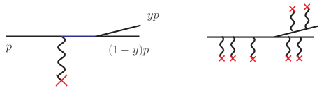
Figure 2: (Left) Schematic of splitting processes after scattering on the thermal bath mediated by a gauge boson. Here the solid lines represent fermions or gauge bosons. The parent particle can shed a large fraction $y$ of its momentum $p$, see eq.(2.4). The small momentum transferred by the intermediate boson implies that the connecting propagator – depicted in blue – is close to the mass shell. (Right) Multiple couplings of the particles involved in the splitting process to the thermal bath of temperature $T$; many soft processes are required for the loss of collinearity and consequently coherence of the splitting process.

However, scattering off the thermal plasma can kick the scattering particle off the mass shell; the outgoing particle can then lose up to half its energy in a $1\rightarrow 2$ splitting process. Fig. 2 (left) shows such a splitting reaction, and defines our convention for the momenta of the participating particles. In contrast to elastic processes, the maximal energy loss is not restricted by the virtuality of either the exchanged gauge boson or of the scattered particle. The daughter particle can therefore carry away a large fraction

$$y\equiv k/p$$ (2.4)

of the parent’s energy, while the virtuality of the intermediate gauge boson is still of the order of its thermal mass given in eq.(2.1). The corresponding small momentum transfer given by eq.(2.2) implies that the virtuality of the scattered particle is also small. Note that the emission of the daughter can in principle proceed via a different interaction, with a coupling $\alpha_{\scriptscriptstyle\rm G^{\prime}}\leq\alpha_{\scriptscriptstyle\rm G}$ than that of the dominant $t-$channel gauge boson exchange.

The most frequent splitting processes are those involving the largest coupling. Their rate is suppressed by a factor $\alpha_{G}$ relative to that for elastic scattering. These higher order processes nevertheless dominate the energy loss since only ${\cal O}\left(\log(p/T)\right)$ of these reactions are required for the thermalization of the parent particle.

Were we to ignore medium effects, we would get the so–called Bethe–Heitler differential rate for these processes:

$$\frac{d\Gamma_{\scriptscriptstyle\rm split}^{\scriptscriptstyle\rm BH}}{d\log{k}}\sim\alpha_{G^{\prime}}\Gamma_{\scriptscriptstyle\rm el}^{s}\leq\alpha_{G}^{2}T\,,$$ (2.5)

corresponding to a time between subsequent splitting reactions $t_{\scriptscriptstyle\rm BH}\equiv{\Gamma_{\scriptscriptstyle\rm split}^{\scriptscriptstyle\rm BH}}^{\scriptscriptstyle\rm-1}$. However, in the rest frame of the thermal medium, the formation time for the splitting process is of order $p/(m_{\rm G}^{\rm th})^{2}$, which is much longer than the time between successive soft elastic scatterings of eq.(2.3) [40]. One should therefore coherently add up all possible contributions to a splitting process, schematically depicted in the right fig. 2. The medium leads to a reduced interaction rate; this is the topic of the next subsection.

2.1 Physics of the LPM suppression

The formal inclusion of the LPM effect requires coherently summing the many ladder diagrams of figure 2, corresponding to extra interaction vertices; this may also be reformulated as a variational problem that is more readily numerically tractable [47, 45]. Alternatively, one may use physical arguments to deduce the parametric form and order–of–magnitude estimate of the LPM suppression for generic processes. In this section, we will keep the species-dependence of the various rates and momentum transfers explicit.

The LPM suppression results from the destructive interference among multiple splitting matrix elements, or equivalently, from the fact that the process is unable to physically distinguish multiple scattering centers in the medium so long as they lie within the coherence region of one another, thereby reducing the effective target density as perceived by the scattering process [40]. The coherence can be understood to last as long as the phase factor accumulated in successive soft scattering reactions is small.

In general, both the emitting and the emitted particle undergo soft scattering reactions on the thermal background. We will work in the rest frame of the thermal bath, which in our application corresponds to the cosmological rest frame. We use coordinates where the parent particle propagates along the $z$ axis, and the splitting occurs at $x^{\mu}_{\rm split}=0$. Denoting the time elapsed traversing the thermal bath by $\delta t$, the trajectory of the emitting particle and the $3-$momentum of a daughter particle of energy $k\gg T$ are then given by

$$\vec{x}(\delta t)\simeq\delta_{t}(\sin\theta\,\hat{e}_{\bot}+\cos\theta\,\hat{e}_{z})\,,\quad\vec{k}\simeq(k_{\parallel}\,\hat{e}_{z}+k_{\bot}\hat{e}^{\prime}_{\bot})\,,$$ (2.6)

where $\hat{e}_{\bot}$ and $\hat{e}^{\prime}_{\bot}$ are (in general independent) unit vectors in the $(x,y)$ plane. Recall that we are interested in collinear splitting. The transverse momentum $k_{\bot}\ll k$ of the daughter as well as the deviation $\theta\ll 1$ of the emitter from the initial $z$ direction therefore only result from the soft interactions shown in fig. 2, so that we can approximate $\sin\theta\simeq\theta,\,\cos\theta\simeq 1-\theta^{2}/2$ and $k_{\parallel}\simeq k-k_{\bot}^{2}/(2k)$.

Crudely, one may say that the coherence, and hence the interference, persists as long as the accumulated phase satisfies

$$\delta\phi=k\cdot x\simeq\delta t\left(-k_{\bot}\theta\hat{e}_{\bot}\cdot\hat{e}^{\prime}_{\bot}+k\frac{\theta^{2}}{2}+\frac{k_{\bot}^{2}}{2k}\right)\leq 1\,.$$ (2.7)

While this condition is satisfied, further splittings are not possible. The angle $\theta\left({\delta t}\right)$ is given by

$$\theta(\delta t)\simeq p_{\bot}(\delta t)/p\,.$$ (2.8)

It is also time dependent. Altogether the accumulated phase is thus of order

$$\delta\phi\sim\delta t\left(\frac{k_{\bot}p_{\bot}}{p}\oplus\frac{kp_{\bot}^{2}}{2p^{2}}\oplus\frac{k_{\bot}^{2}}{2k}\right)\,.$$ (2.9)

The $\oplus$ symbol indicates that the terms should be added in quadrature in a statistical sense, since in general the emitter and both emitted particles undergo a random walk through multiple scatters on the thermal background. During a time span $\delta t$ there will be $\delta t/\delta t_{\rm el}$ “steps”, with “step size” $\delta k_{\rm el}$. If both particles interact with similar strength, we thus have

$$\left\langle k_{\bot}\right\rangle(\delta t)\simeq\left\langle p_{\bot}\right\rangle\simeq\sqrt{\frac{\delta t}{\delta t_{\scriptscriptstyle\rm el}}}\,\delta k_{\scriptscriptstyle\rm el}\simeq{\delta t}^{1/2}\Gamma_{\scriptscriptstyle\rm el}^{1/2}\delta k_{\scriptscriptstyle\rm el}\,.$$ (2.10)

For very hard splitting, where $k\sim p$, all three terms in eq.(2.9) will then be of the same order. However, in the more likely configuration where $k\ll p$ the third term dominates. For the case where all particles that participate in the splitting have roughly equal coupling strength to the thermal bath, we can thus approximate the phase $\delta\phi\sim\delta tk_{\bot}^{2}/k$, with the understanding that $k$ denotes the momentum of the softer daughter particle. The coherence time, defined by $\delta\phi(t_{\rm coh})=1$, is then given by

$$\delta t_{\scriptscriptstyle\rm coh}\sim\sqrt{\frac{k}{\Gamma_{\scriptscriptstyle\rm el}\delta k_{\scriptscriptstyle\rm el}^{2}}}\,,$$ (2.11)

where we have used eq.(2.10). Recall that the next splitting reaction can only happen at $t>\delta t_{\scriptscriptstyle\rm coh}$; this can be described by reducing the plasma density and therefore the interaction rate by a factor

$$R_{\scriptscriptstyle\rm LPM}(k)\simeq\delta t_{\scriptscriptstyle\rm coh}^{-1}\delta t_{\scriptscriptstyle\rm el}=\sqrt{\frac{\delta k_{\scriptscriptstyle\rm el}^{2}}{k\Gamma_{\scriptscriptstyle\rm el}}}\,.$$ (2.12)

Please note that this suppression factor scales like $1/\sqrt{k}$, which favors softer splittings due to their shorter coherence time.

Recall, however, that we have assumed equal interaction strengths for all three particles participating in the splitting process. Let us now consider the case where the emitted particle basically does not couple to the thermal bath, as in $q\rightarrow\gamma q$. In the particular case of an Abelian gauge boson, the absence of $t-$channel soft scattering processes on the thermal bath implies that its momentum can be considered a constant (originating from the splitting process itself). We can then choose its direction, rather than that of the parent particle, to define the $z$ axis, i.e. $k_{\bot}=0$. In this case, only the second term in eq.(2.9) survives. Again defining the coherence time via $\delta\phi(\delta t_{\rm coh})=1$ and using eq.(2.10) for $p_{\bot}$ we now have

$$\delta t_{\scriptscriptstyle\rm coh}\sim\sqrt{\frac{p^{2}}{k\Gamma_{\scriptscriptstyle\rm el}(\delta k_{\scriptscriptstyle\rm el})^{2}}},\quad R_{\scriptscriptstyle\rm LPM}(k)\sim\sqrt{\frac{k\delta(k_{\scriptscriptstyle\rm el})^{2}}{p^{\scriptscriptstyle\rm 2}\Gamma_{\scriptscriptstyle\rm el}}}.$$ (2.13)

Evidently, the LPM effect favors the emission of harder photons, in contrast to what we had in (2.12) for gluon emission. This stark difference can be understood from the observation that a harder photon implies a softer second daughter particle, whose soft elastic scatterings with the plasma can therefore result in a faster growth of $\theta$ and hence earlier loss of coherence.

Before we move on to presenting explicit expressions for the LPM–corrected rates, calculated in the literature, and for the many available processes of the standard model fermions and gauge bosons, we may summarize the results of our physical arguments for the LPM suppressed splitting rate as follows. The rate for a process can be decomposed as the result of the splitting rate in vacuum, using the thermal gauge boson mass (2.1) as infrared regulator, and the corresponding LPM suppression factor:

$$\frac{d\Gamma^{\rm split}_{\scriptscriptstyle\rm LPM}\left(s(p)\rightarrow s^{\prime}(k)+s^{\prime\prime}(p-k)\right)}{dk}=\frac{d\Gamma^{\rm split}_{\scriptscriptstyle\rm vac}\left({s(p)\rightarrow s^{\prime}(k)+s^{\prime\prime}(p-k)}\right)}{dk}\times R_{\scriptscriptstyle\rm LPM}\left({k,s^{\prime}}\right)\,,$$ (2.14)

where

$$R_{\scriptscriptstyle\rm LPM}\left({k}\right)\propto\left\{\begin{aligned} &\sqrt{\frac{kT}{p^{2}}}&&s^{\prime}=\texttt{Abelian GB}&\\ &\sqrt{\frac{T}{\min{\left({k,p-k}\right)}}}&&\texttt{others}&\end{aligned}\right..$$ (2.15)

Here $s$ is the parent particle and $s^{\prime},\,s^{\prime\prime}$ are the two daughter particles.

Of course, the heuristic derivation given here does not allow to derive exact numerical factors. In particular, we have assumed that the transverse momentum due to the splitting itself is no larger than $\delta k_{\rm el}$. The inclusion of processes with momentum transfer $q>\delta k_{\rm el}$ enhances the final splitting rate by a so–called Coulomb logarithm of order $\ln(p/T)$. Once this factor is included, we will see in the next subsection that the results of careful calculations indeed approximately reproduce the behavior given by eqs.(2.14) and (2.15).

2.2 LPM suppressed splitting rates in leading logarithmic approximation

As mentioned earlier, the study of relativistic heavy ion collisions requires knowledge of various elastic $2\rightarrow 2$ scattering as well as splitting processes, where the inclusion of coherence effects is crucial. We mostly rely on the results obtained in [42], whose notation we follow; we, however, generalize the results to allow for two separate gauge groups being responsible for the splitting process and the gauge-mediated scattering of the three particles of the thermal bath. We also discuss the proper choice of parameters corresponding to each of these two gauge groups. Note that we are interested in the splitting rate per parent particle, while in the literature the total emission of daughter particles per time and volume is often given [47, 45, 46]. Moreover, we neglect all Bose enhancement and Fermi blocking factors; this is justified since we are only interested in particles with energy much above $T$, which have very low occupation numbers.

To be precise, the LPM corrected rate for the various splitting reactions can be written as

$$\frac{d\Gamma^{\scriptscriptstyle\rm split}_{\scriptscriptstyle\rm LPM}\left({s(p)\rightarrow s^{\prime}(k)+s^{\prime\prime}(p-k)}\right)}{dy}=\frac{(2\pi)^{3}}{p\nu_{s}^{G}}\,\gamma_{s\rightarrow s^{\prime}s^{\prime\prime}}\left({p,yp,(1-y)p}\right)\,.$$ (2.16)

Here $y$ is the momentum fraction carried by the species $s^{\prime}$ as in eq.(2.4), and $\nu_{s}^{G}$ is the number of spin degrees of freedom for the species $s$ times $d^{\scriptscriptstyle\rm G}_{s}$, the dimension of its gauge representation under the gauge group $G$. For example, a gluon has $\nu_{g}^{SU(3)}=2\times 8=16$, and a quark has $\nu_{q}^{SU(3)}=6,\,\nu_{q}^{SU(2)}=4$.

The bulk of information about the splitting process is encoded the in the splitting functions $\gamma_{s\rightarrow s^{\prime}s^{\prime\prime}}\left({p;yp,(1-y)p}\right)$. Here $s,s^{\prime}$ and $s^{\prime\prime}$ stand for either a fermion $F$ or a gauge boson $A$. To leading logarithmic approximation, they are given by [42]:

$$\gamma_{A\rightarrow AA}(p;yp,(1-y)p) =\frac{d_{A}^{G^{\prime}}C_{A}^{G^{\prime}}\alpha_{G^{\prime}}}{(2\pi)^{4}\sqrt{2}}\frac{1+y^{4}+(1-y)^{4}}{y^{2}(1-y)^{2}} \cdot \left[m_{\scriptscriptstyle\rm th}^{2}\,\hat{\mu}_{\perp}^{2}(1,y,1{-}y;A,A,A)\right]_{G}\,;$$ (2.17a)

$$\gamma_{F\rightarrow AF}(p;yp,(1-y)p) =\frac{d_{F}^{G^{\prime}}C_{F}^{G^{\prime}}\alpha_{G^{\prime}}}{(2\pi)^{4}\sqrt{2}}\frac{1+(1-y)^{2}}{y^{2}(1-y)} \cdot \left[\,m_{\scriptscriptstyle\rm th}^{2}\,\hat{\mu}_{\perp}^{2}(1,y,1{-}y;F,A,F)\right]_{G}\,;$$ (2.17b)

$$\gamma_{A\rightarrow FF}(p;yp,(1-y)p) =\frac{d_{F}^{G^{\prime}}C_{F}^{G^{\prime}}\alpha_{G^{\prime}}}{(2\pi)^{4}\sqrt{2}}\frac{y^{2}+(1-y)^{2}}{y(1-y)}\times N_{fl} \cdot \left[m_{\scriptscriptstyle\rm th}^{2}\,\hat{\mu}_{\perp}^{2}(1,y,1{-}y;A,F,F)\right]_{G}\,.$$ (2.17c)

Here we have again labeled with $G$ the gauge group responsible for the (dominant) scattering processes on the thermal background, while gauge group $G^{\prime}$ is responsible for the splitting. In our numerical analysis we will ignore subdominant contributions to the soft scattering; e.g. we will only include gluon exchange for the soft scattering of quarks. In contrast, the gauge group $G^{\prime}$ is determined uniquely by the identity of the involved gauge boson(s). In detail, eqs.(2.17a), (2.17b) and (2.17c) describe pure gauge splittings like $g\to gg$ or $W\to WW$, gauge boson emission from a fermion like $q\to gq$ or $l\to Wl$, and splitting of a gauge boson to a fermion antifermion pair like $g\to q\bar{q}$ or $W\to l\bar{l}$, respectively; of course, $\gamma_{A\rightarrow AA}=0$ for $U(1)$ interactions.

The first term in each splitting function captures the physics of the splitting process without the plasma effects, and thus loosely corresponds to $\Gamma_{\scriptscriptstyle\rm vac}$ in (2.14). The representation dimension $d_{s}^{\scriptscriptstyle\rm G^{\prime}}$ was introduced below equation (2.16), and the remaining parameter $C_{s}^{\scriptscriptstyle\rm G^{\prime}}$ is the quadratic Casimir. Within the SM, with the fermions and bosons in fundamental and adjoint representations respectively, we have for the group $SU(N)$:

$$C_{F}=\left({N^{2}-1}\right)/2N\,,\qquad C_{A}=N\,,\qquad d_{F}=N\,,\qquad d_{A}=N^{2}-1,$$ (2.18)

while for a $U(1)$, we have

$$C_{F}^{\scriptscriptstyle\rm s}=Y_{s}^{2},\qquad C_{A}=0\,,\qquad d_{F}=1,\qquad d_{A}=1\,,$$ (2.19)

with $Y_{s}$ the $U(1)$ charge of the corresponding fermion.

The $y$ dependence of the different fragmentation functions is determined by the structure of the relevant three–point vertex; up to a factor $1/[y(1-y)]$ it is the same as that of the splitting functions appearing in the famous DGLAP equations [51, 52, 53]. The parameter $N_{fl}$ in eq.(2.17c) quantifies the number of indistinguishable Dirac fermions that the gauge boson $A$ can split into. For the $SU(2)$ and $U(1)_{Y}$ gauge bosons splitting into $q\bar{q}$ pairs this will always include a color factor of $3$; $N_{fl}$ may be larger if several quarks (of different generations, say) are considered indistinguishable.

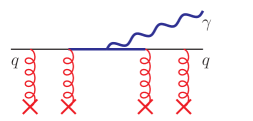
Figure 3: Photon bremsstrahlung (blue, $G^{\prime}=U(1)_{\scriptscriptstyle\rm EM}$) from a quark interacting strongly with colored plasma particles (red, $G=SU(3)_{C}$). The resulting rate is of order $\alpha_{G}\alpha_{G^{\prime}}$.

The second sets of terms in eqs.(2.17), denoted by the subscript $\left[\ldots\right]_{G}$, can be thought of as representing the background plasma of temperature $T$, describing the scattering target density, the momentum transfer for the $2\rightarrow 3$ scattering process, as well as the coherent suppression effects. Before moving on to the individual elements, let us take a moment to clarify the assignment of $G$. Take as an example the physical process of emission of a photon from a QGP via the splitting process $q\to\gamma q$ depicted in figure 3. In the previous part, we assigned $G^{\prime}=U(1)_{\scriptscriptstyle\rm EM}$ as the gauge group responsible for the emission of the photon, corresponding to the blue sections of figure 3. This splitting process however relies on the interactions with the hot plasma; the same interactions also provide the coherent suppression effect, shown in red in figure 3. As can be seen, the latter class of processes will be dominated by the strong interactions of the colored quarks, so that $G=SU(3)_{C}$ but with $C_{\gamma}=0$. Note that we ignore electroweak interactions of the quarks with the background plasma in this treatment; similarly, we ignore hypercharge interactions of $SU(2)$ doublet leptons with the background. In this approximation only a single group $G$ contributes to the loss of coherence.

The exact leading order expression for the thermal mass of the gauge boson, whose order of magnitude has been given in eq.(2.1), is [42]

$$m^{2}_{G,{\rm th}}=\frac{1}{3}g_{G}^{2}T^{2}\left(C_{A}^{G}+\sum_{f}\frac{d_{f}}{d_{A}}N_{f}C_{F}^{G}\right)\,,$$ (2.20)

where $N_{f}$ is the total number of Dirac fermions with a gauge representation corresponding to $C_{F}$; see eqs.(2.18) and (2.19) for groups $SU(N)$ and $U(1)$, respectively. In these terms, the function $\hat{\mu}_{\perp}^{2}$ on the right–hand side (RHS) of eqs.(2.17) can in leading log approximation be universally written as [42]

$$\hat{\mu}_{\perp}^{2}(y_{1},y_{2},y_{3};s_{1},s_{2},s_{3})\simeq\frac{g_{G}T}{m_{G,{\rm th}}}\left[\frac{2}{\pi}\,y_{1}y_{2}y_{3}\,\frac{p}{T}\right]^{1/2}\Biggl{\{}\Biggl{[}\tfrac{1}{2}(C_{s_{2}}+C_{s_{3}}-C_{s_{1}})y_{1}^{2}+\tfrac{1}{2}(C_{s_{3}}+C_{s_{1}}-C_{s_{2}})y_{2}^{2}$$

$$\hskip 150.00023pt+\tfrac{1}{2}(C_{s_{1}}+C_{s_{2}}-C_{s_{3}})y_{3}^{2}\Biggr{]}\ln(\sqrt{p/T})\Biggr{\}}^{1/2}\,.$$ (2.21)

Equation (2.2) encodes the LPM effect for a splitting process $s_{1}\rightarrow s_{2}s_{3}$; the various Casimir factors represent the coupling of the three particles involved in the thermal plasma to the thermal bath. The coupling constant $g_{G}$ cancels in eq.(2.2) due to $m_{G,{\rm th}}$ appearing in the denominator, see eq.(2.20).

We may now see how the explicit form of eq.(2.2) reproduces our physically motivated results for both cases in eqs.(2.12) and (2.13). Consider, first, the photon emission process discussed in section 2.1. As emphasized above, the photon has $C_{s2}=C_{A}=0$, while $C_{s1}=C_{F}=C_{s3}=4/3$ for the colored quarks, so that

$$\hat{\mu}_{\perp}^{2}(1,y,1-y;q,\gamma,q)\propto\left[\frac{2}{\pi}\,y(1-y)\,\frac{p}{T}\right]^{1/2}\Biggl{\{}\frac{4}{3}y^{2}\ln(\sqrt{p/T})\Biggr{\}}^{1/2}\,.$$ (2.22)

On the other hand, for gluon emission from a quark, $q\to gq$, we have $C_{s2}=C_{A}=3$, and $C_{s1}=C_{F}=C_{s3}=4/3$, so that

$$\hat{\mu}_{\perp}^{2}(1,y,1-y;q,g,q)\propto\left[\frac{2}{\pi}\,y(1-y)\,\frac{p}{T}\right]^{1/2}\Biggl{\{}\Biggl{[}\frac{4}{3}y^{2}+3\left(1+(1-y)^{2}\right)\Biggr{]}\ln(\sqrt{p/T})\Biggr{\}}^{1/2}\,.$$ (2.23)

For small $y$, where the term in the second square parentheses in eq.(2.23) approaches a constant, eqs.(2.22) and (2.23) differ by factor $y=k/p$, reproducing the relation between eqs.(2.12) and (2.13). Finally, the appearance of the Coulomb logarithm is, as mentioned before, the result of including all process with a momentum transfer larger than $m_{\scriptscriptstyle\rm th}$, which occur at a rate smaller than that of eq.(2.3).

Before concluding this subsection we comment on processes where two participants carry color but the third one only undergoes weaker non–Abelian interactions. Within the SM, the only such processes involve two $SU(2)$ doublet quarks and an $SU(2)$ gauge boson. An example is $q\to Wq$ splitting, which is described by eq.(2.17b) with $G^{\prime}=SU(2),\,G=SU(3)_{C}$. Recall that we simply set $C_{A}=0$ when treating the emission of a $U(1)$ gauge boson, which cannot scatter on the background by $t-$channel exchange of a gauge boson. On the other hand, the non–Abelian $W$ will have such interactions. Of course, the relevant $SU(2)$ coupling strength is significantly smaller than that of $SU(3)$. Nevertheless, the discussion at the end of sec. 2.1 showed that the scattering of the $W$ might terminate coherence if it has much less energy than the parent quark. We treat this by assigning $C_{A}=(\alpha_{W}/\alpha_{S})C_{A}^{W}$ to the $W$ boson in the splitting process. This may be a crude approximation, but we do not know of a study focusing on the calculation of the LPM effect involving multiple gauge groups. Moreover, as we will see in sec. 3, the energy loss of the original parent particle, and hence the spectrum of all daughter particles, is mostly determined by more symmetric splittings, where the difference between $C_{A}=0$ and $0<C_{A}\ll 1$ is small.

2.3 Particle content and the treatment of chirality

Equations (2.17) and (2.2) provide the rate of all splitting processes involving SM fermions and gauge bosons. Before we move on to composing the system of Boltzmann equations, however, we should address some technicalities regarding the applicability of the splitting rates to various processes.

The formalism we adopt here has been developed for QCD interactions, which are vector–like. As already noted, the standard model being a chiral theory, we will keep track of the chiralities of the fermions in the splitting cascade.

Since we always sum or average over the spins of the participating gauge bosons, we do not need to change the $y$ dependence of any splitting function. Moreover, the $1/2$ factors in the normalization of $\nu$ in eq.(2.16) and of $d_{F}$ in eq.(2.17b) cancel each other so that no change is required for the case of gauge boson emission off a chiral fermion. However, since $N_{fl}$ in eq.(2.17c) counts the number of indistinguishable Dirac fermions, it should include a factor of $1/2$ when considering species of chiral (or Weyl) fermions.

Note that the gauge boson vertices are chirality conserving. The relaxation of any preexisting net chiral charge via $2\rightarrow 2$ or $1\rightarrow 2$ processes will therefore rely on bare fermion mass insertions [55, 54], which are absent in the unbroken $SU(2)$-phase, or involve emission or exchange of a scalar Higgs boson; the latter processes are highly suppressed by the small Yukawa couplings of most SM fermions, as well as by a factor of $y^{2}/2$ in the splitting function relative to that for the emission of a gauge boson [56, 57]. In what follows, we will therefore treat the chiralities of fermions as conserved quantities, i.e. we will present separate spectra for left– and right–chiral fermions $f_{L/R}$.

Somewhat trivially, one does not need to distinguish between the members of a given representation of the gauge group. As an example, in the phase of unbroken $SU(2)$ we would not, and in fact cannot, distinguish between an up–type and a down–type left–chiral fermion. Even if we fix the gauge (so that “up–type” is well defined), $2\to 2$ scattering processes on the thermal background induce changes between these states at the high rate $\Gamma_{\scriptscriptstyle\rm el}$, i.e. these states are not well–defined over the duration of a splitting process. The same is also true for the color of a quark, so that the quark undergoing a splitting process in figure 2 cannot be considered to have a well–defined color even in a fixed gauge.

However, at least in principle different right–chiral fermions $f_{R}$ are physically distinct particles. For example, $u_{R}$ and $d_{R}$ have different $U(1)_{Y}$ charges. However, as it is difficult to imagine physical scenarios where we would need to distinguish between the up and down type $f_{R}$, we will simply treat both these species as possessing an average squared charge in (2.19), using

$$Y_{q_{R}}^{2}=\frac{1}{2}\left({Y^{2}_{u_{R}}+Y^{2}_{d_{R}}}\right)\,.$$ (2.24)

Moreover, we will not distinguish between fermions of different generations This still leaves us with seven distinct particle species:

$$s\in\left\{q_{L},\,q_{R},\,\ell_{L},\,\ell_{R},\,g,\,W,\,B\right\}\equiv\mathbb{S}.$$ (2.25)

Note also that we assume equal production of particles and antiparticles. This is true if the original $M$ particles always decay into $s\bar{s}$ pairs. Treating more fermion species as distinguishable is in principle straightforward. However, this would increase the number of coupled Boltzmann equations that need to be solved, and also the number of terms in some of these equations. The choice (2.25) should be sufficient to illustrate the main effect of the appearance of particles with very different interaction strengths in this first, exploratory analysis.

3 System of Boltzmann equations

We established in section 2 that $2\to 3$ processes play a significant role in the redistribution of energy, and in the growth of number density, towards a thermal distribution. These can be understood as quasi–elastic scattering processes that leave the energy $p$ of the parent particle almost unchanged, followed by $1\to 2$ splitting which distributes the energy of the parent among two daughter particles of energy $k$ and $p-k$, respectively. The rate of this $2\rightarrow 3$ process, differential in the energy of one of the daughters, is given by eq.(2.16).

Our final goal is to find the number densities of all particles that are not in thermal equilibrium during the thermalization cascade. These densities are governed by a set of Boltzmann equations. In order to introduce the framework and our notation, it might be beneficial to first briefly review the treatment of a pure gauge theory where one only has to consider a single species of particle, as done in [36, 18].

3.1 Pure gauge cascade

The time dependence of the phase space distribution of a particle species is, as usual, given by a Boltzmann equation. The well–motivated assumptions of homogeneity and isotropy imply that the phase space or number density depends solely on the magnitude $p$ of the $3-$momentum and on the cosmological time $t$. Splittings of the the species $s$ generate a non–thermal spectrum, which we denote by

$$\tilde{n}_{s}\left({p}\right)\equiv\frac{dn_{s}(p)}{dp}\quad\texttt{such that}\quad\int_{T}^{p_{\rm max}}\tilde{n}_{s}(p)dp=n_{s}\,.$$ (3.1)

The generic Boltzmann equation governing this number density reads

$$\frac{\partial}{\partial t}\tilde{n}_{s}(p,t)-3Hp\frac{\partial}{\partial p}\tilde{n}_{s}(p,t)=+\mathcal{C}{\scriptscriptstyle\rm inj}(p,t)-\mathcal{C}{\scriptscriptstyle\rm dep}(p,t).$$ (3.2)

The two collision terms on the RHS represent injection processes adding particles of momentum $p$ and depletion processes removing particles of momentum $p$, respectively. As a typical primary injection process, we consider the decay of a long–lived matter particle of mass $M$, so that $p_{\rm max}=M/2$. The injection also includes the “feed-down” from particles with momentum $k>p$ through their splittings. In general, the form of the initial injection spectrum will be model dependent. Without loss of generality, however, we may assume the matter particle to decay to two initial particles, so that the initial injection can be written as $\delta-$function contribution at $p=M/2$. Since the Boltzmann equation is linear in $\tilde{n}_{s}$, the result for any other injection spectrum can be obtained by convoluting this initial spectrum with the final spectrum of non–thermal particles resulting from the initial delta function.

It can be shown that in almost all scenarios of interest the initial particles thermalize within a time which is much shorter than a Hubble time [35, 36]. This means that the term $\propto H$ in eq.(3.2) can be neglected; furthermore, the temperature of the thermal bath can be considered as constant within the thermalization time. Injection and depletion will then quickly reach equilibrium, as long as new particles with initial energy $M/2$ keep being injected. This (quasi) steady–state solution satisfies

$$\mathcal{C}{\scriptscriptstyle\rm dep}(p)=\mathcal{C}{\scriptscriptstyle\rm inj}(p).$$ (3.3)

The exchange symmetry of the two daughter states for the case of $g\to gg$ splittings, see eq.(2.17a), allows one to write eq.(3.3) as

$$2n_{\scriptscriptstyle\rm M}\Gamma_{\scriptscriptstyle\rm M}\delta(p-M/2) +\int_{p+\kappa T}^{M/2}\tilde{n}_{s}(k)\frac{d\Gamma^{\rm split}_{\scriptscriptstyle\rm LPM}(s(k)\to s(p)s(k-p))}{dp}dk$$

$$=\int_{\kappa T}^{p/2}\tilde{n}_{s}(p)\frac{d\Gamma^{\rm split}_{\scriptscriptstyle\rm LPM}(s(p)\to s(k)s(p-k))}{dk}dk\,.$$ (3.4)

Here $n_{\scriptscriptstyle\rm M}$ and $\Gamma_{\scriptscriptstyle\rm M}$ denote the number density and decay rate of the long–lived matter particle, and the splitting rates on both LHS and RHS are given by eqs.(2.16) and (2.17a). We have used $\kappa T$ as an infrared (IR) cutoff for the $2\rightarrow 3$ processes, where $\kappa$ is of order unity. This is reasonable since the much faster $2\rightarrow 2$ scattering reactions allow momentum exchange of order $T$; moreover, the total spectrum of particles with energy $\leq 3T$ is in any case dominated by the thermal contribution. It has been shown [36] that the precise choice of $\kappa$ does not affect the physical solution for $p\gg T$, and so we may choose $\kappa=1$ for convenience. The choice of an IR cutoff further allows for a straightforward numerical solution of eq.(3.1).

This numerical solution is facilitated by introducing

$$\widetilde{N}_{\scriptscriptstyle\rm M}=\frac{2n_{\scriptscriptstyle\rm M}\Gamma_{\scriptscriptstyle\rm M}}{\Gamma^{\rm split}_{\scriptscriptstyle\rm LPM}(M/2)}\,,\quad\bar{n}_{s}\left({p}\right)=\frac{\tilde{n}_{s}\left({p}\right)}{\tilde{N}_{\scriptscriptstyle\rm M}},$$ (3.5)

and further using the dimensionless quantities

$$x=\frac{p}{T}\,\implies\bar{n}_{s}\left({x}\right)=T\bar{n}_{s}\left({p}\right)\,.$$ (3.6)

If the coupling is treated as a constant, the spectrum $\bar{n}(x)$ can only depend on the single parameter

$$x_{\scriptscriptstyle\rm M}=\frac{M}{2T}\,.$$ (3.7)

The Boltzmann equation (3.1) can now be written as

$$\bar{n}_{s}(x;x_{\scriptscriptstyle\rm M})=\int_{x+\kappa}^{x_{\scriptscriptstyle\rm M}}\frac{\bar{n}_{s}(x^{\prime})}{\Gamma^{\rm split}_{\scriptscriptstyle\rm LPM}\left({s(x)\to ss}\right)}\frac{d\Gamma^{\rm split}_{\scriptscriptstyle\rm LPM}\left({s(x^{\prime})\to s(x)s(x^{\prime}-x)}\right)}{dx}dx^{\prime}+\delta(x-x_{\scriptscriptstyle\rm M})\,.$$ (3.8)

Here $\Gamma^{\rm split}_{\scriptscriptstyle\rm LPM}\left({s(x)\to ss}\right)$ is the total (integrated) rate for a particle of dimensionless momentum $x$ to undergo a splitting process. Note that the splitting rate appears in both the numerator and denominator of eq.(3.8), so that numerical factors like $\sqrt{\tilde{g_{*}}^{s}}$ as well as the coupling strength $\alpha_{G}$ do not affect $\bar{n}_{s}\left({x}\right)$; they appear in the final, physical spectrum only via the normalization factor $\tilde{N}_{\scriptscriptstyle\rm M}$.

The numerical solution of eq.(3.8) can be approximated by [36]

$$\bar{n}_{s}(x;x_{\scriptscriptstyle\rm M})=\delta(x-x_{\scriptscriptstyle\rm M})+\frac{\left[a\left(x/x_{\scriptscriptstyle\rm M}\right)^{-3/2}\left(1-x/x_{\scriptscriptstyle\rm M}\right)^{-b}+c\right]\left(1-2/\sqrt{x_{\scriptscriptstyle\rm M}}\right)}{\sqrt{x_{\scriptscriptstyle\rm M}}\left(1-\sqrt{2/x}\right)^{5/4}}\,,$$ (3.9)

with $a,\,b,\,c\approx 1/2$. The form of the single species solution (3.9) shows that for $x_{\scriptscriptstyle\rm M}>x\gg 1$, the solution is proportional to the function

$$f\left({x/x_{\scriptscriptstyle\rm M}}\right)\equiv\left[a\left(x/x_{\scriptscriptstyle\rm M}\right)^{-3/2}\left(1-x/x_{\scriptscriptstyle\rm M}\right)^{-b}+c\right]\,,$$ (3.10)

which depends only on the ratio $x/x_{\scriptscriptstyle\rm M}$. In section 4 we will use this latter feature, and the pure–gauge solution to present the results of the splitting cascade involving all species $s\in\mathbb{S}$.

3.2 Multiple species and the coupled set of integral equations

So far we have assumed that the parent particle of species $s$ can only split into two daughter particles of the same species, as is the case for a pure Yang–Mills gauge theory. The splitting of a gluon into two gluons is indeed the fastest splitting reaction in the SM, and is expected to dominate the evolution of the system produced in heavy ion collisions, at least at central rapidities [49]. However, the multiplicity of accessible fermion flavors suggests that a sizable population of fermionic daughters develops in the splitting cascade. Since SM quarks are charged under several gauge groups, eventually electroweak gauge bosons, and hence leptons, will become part of the cascade even when starting from a parent gluon. Moreover, the matter particles whose decays feed the cascade might primarily decay to colorless species. Recall finally that the purpose of computing the spectrum of particles in the cascade triggered by the primary decay is to compute rates for processes that leave observable relics, e.g. dark matter particles or a baryon asymmetry; and these reactions may involve preferentially, or even only, colorless particles in the initial state. Hence a treatment including all SM species is necessary.

We will therefore extend the previous studies by formulating and solving the coupled system of Boltzmann equations governing the energy spectrum of all particles listed in eq.(2.25) during a LPM–suppressed thermalization cascade. As in subsec. 3.1 we will be interested in the quasi steady–state solution. The spectrum of particles of species $s$ is then determined by the integral equation

$$2n_{\scriptscriptstyle\rm M}\Gamma_{\scriptscriptstyle\rm M}Br_{s}\cdot\delta(p-M/2) + \sum_{s^{\prime},s^{\prime\prime}}\int_{p+\kappa T}^{M/2}\tilde{n}_{\scriptscriptstyle\rm s^{\prime}}(k)\frac{d\Gamma^{\rm split}_{\scriptscriptstyle\rm LPM}(s^{\prime}(k)\rightarrow s(p)s^{\prime\prime}(k-p))}{dp}dk$$ (3.11)

$$= \sum_{s^{\prime},s^{\prime\prime}}\int_{\kappa T}^{p-\kappa T}\tilde{n}_{s}(p)\frac{d\Gamma^{\rm split}_{\scriptscriptstyle\rm LPM}(s(p)\rightarrow s^{\prime}(k)s^{\prime\prime}(p-k))}{dk}dk\,.$$

Here $2Br_{s}$ is the average number of $s$ particles produced in a given decay of an $M$ particle. As noted earlier, we assume equal production of fermions and antifermions, and the density $n_{s}$ in fact includes $s$ and $\bar{s}$ particles if these are distinct. In the rate $\Gamma^{\scriptscriptstyle\rm split}_{\scriptscriptstyle\rm LPM}\left({s(p)\rightarrow s^{\prime}(k)s^{\prime\prime}(p-k)}\right)$ the particle type of $s^{\prime\prime}$ is often fixed once $s$ and $s^{\prime}$ have been specified; this is true in particular if $s$ and/or $s^{\prime}$ denotes a gauge boson. However, if $s$ and $s^{\prime}$ are both fermions (which implies $s=s^{\prime}$), several types of gauge boson might be possible for $s^{\prime\prime}$; for $q_{L}\rightarrow q_{L}$ splitting, $\sum_{s^{\prime\prime}}$ will even run over all three species of gauge bosons of the SM.

In eq.(3.11) most dependence on high–scale physics has been factored into the first term. In particular, the product $n_{\rm M}\Gamma_{\rm M}$ only affects the overall normalization of all spectra. In contrast, the splitting rates can be computed within the theory that is valid at energy scales well below $M$, which we assume to be the SM. The second and third term in eq.(3.11), which determine the shapes of the various spectra and also affect their relative normalization, therefore depend on high–scale physics only through the upper limit of integration of the first integral. As in the case of the single particle cascade, it is useful to make these dependencies explicit by using (3.6) to rewrite (3.11) in the dimensionless form

$$\bar{n}_{s}(x) = \frac{\Gamma^{\rm split}_{\scriptscriptstyle\rm LPM}\left({s^{*},x_{\scriptscriptstyle\rm M}}\right)}{\Gamma^{\rm split}_{\scriptscriptstyle\rm LPM}\left({s,x_{\scriptscriptstyle\rm M}}\right)}Br_{s}\cdot\delta\left({x-x_{\scriptscriptstyle\rm M}}\right)$$ (3.12)

$$+ \sum_{s^{\prime},s^{\prime\prime}}\int_{x+\kappa}^{x_{\scriptscriptstyle\rm M}}\frac{\bar{n}_{\scriptscriptstyle\rm s^{\prime}}\left({x^{\prime}}\right)}{\Gamma^{\rm split}_{\scriptscriptstyle\rm LPM}\left({s,x}\right)}\frac{d\Gamma^{\rm split}_{\scriptscriptstyle\rm LPM}\left({s^{\prime}(x^{\prime})\rightarrow s(x)s^{\prime\prime}(x^{\prime}-x)}\right)}{dx}dx^{\prime}\,.$$

Here we have generalized eq.(3.5) by normalizing the spectra of all species using the total rate of $2\rightarrow 3$ reactions of some reference species $s^{*}$:

$$\widetilde{N}^{*}_{\scriptscriptstyle\rm M}=\frac{2n_{\scriptscriptstyle\rm M}\Gamma_{\scriptscriptstyle\rm M}}{\Gamma^{\rm split}_{\scriptscriptstyle\rm LPM}(s^{*},M/2)}\,,\quad\bar{n}_{s}(x)=T\bar{n}_{s}\left({p}\right)=T\frac{\tilde{n}_{s}\left({p}\right)}{\tilde{N}_{\scriptscriptstyle\rm M}^{*}}\,,$$ (3.13)

with

$$\Gamma^{\rm split}_{\scriptscriptstyle\rm LPM}(s,x)=\sum_{s^{\prime},s^{\prime\prime}}\int_{\kappa}^{x-\kappa}\frac{d\Gamma^{\rm split}_{\scriptscriptstyle\rm LPM}\left({s(x)\rightarrow s^{\prime}(x^{\prime})s^{\prime\prime}(x-x^{\prime})}\right)}{dx^{\prime}}dx^{\prime}\,.$$ (3.14)

We use the particle with the largest total rate, i.e. the gluon $s^{*}=g$, for the normalization.

In a single particle cascade, increasing the coupling strength increases the total rate for $2\rightarrow 3$ reactions which reduces the overall normalization of the spectrum. The reason is that a larger rate of splitting reactions decreases the thermalization time, i.e. the particle spends less time in the cascade. In the case at hand, this is true only if all couplings are increased by the same factor. In contrast, increasing some coupling relative to that of the reference particle (i.e. relative to the QCD coupling, for our choice $s^{*}=g$) still reduces the normalization of the first term in eq.(3.12), but it also increases the probability that $s$ will be produced later in the cascade.

4 Numerical calculation of the spectra

The numerical solution of eq.(3.12) proceeds essentially in the same way as in the case of a single particle cascade: one starts at $x=x_{\scriptscriptstyle\rm M}$ (regularizing the $\delta$ function [36]) and successively works down to lower $x$. Of course, now we actually need to solve seven such equations, for the species listed in eq.(2.25).

The integrand in eq.(3.12) is computed from eqs.(2.16) and (2.17), using eqs.(2.18) and (2.19) for the coupling parameters; we use three generations of massless leptons and quarks, and include extra factors of $1/2$ for splitting of gauge bosons to chiral fermion pairs in (2.17). The contributing splitting reactions are depicted in fig. 4. Note that we use the parameter $x$ of eq.(3.6) in the Boltzmann equations, while the fragmentation functions are written in terms of the momentum fraction $y$ of eq.(2.4); the two are related by $y=k_{\scriptscriptstyle\rm daughter}/p_{\scriptscriptstyle\rm parent}=x_{\scriptscriptstyle\rm daughter}/x_{\scriptscriptstyle\rm parent}$. The use of the exact (leading order) splitting functions (2.17) implies that the total rates $\Gamma^{\rm split}_{\scriptscriptstyle\rm LPM}(s,x)$ also have to be computed numerically, whereas the approximations used in ref.[36] allowed the integral in eq.(3.14) to be calculated analytically.

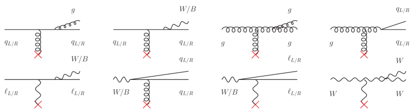
Figure 4: Splitting processes for the species in $\mathbb{S}$ that can proceed via soft interactions with the thermal background. The red crosses again denote couplings to particles in the thermal bath via many soft exchanges. We only include the $t-$channel gauge boson which has the largest possible coupling, as discussed in section 2.2; e.g. the process $B\to\ell_{L}\ell_{L}$ is mediated by an $SU(2)$ gauge boson $W$. Note also that $W$ bosons only couple to left–handed fermions $q_{L},\,\ell_{L}$.

In our numerical work, we will assume that only one of the seven species $I\in\mathbb{S}$ is produced in primary $M$ decays, i.e. $Br_{I}=1$, in which case the first term in eq.(3.12) is absent for the other species, $Br_{s}=0\ \forall s\neq I$. We denote the resulting scaled number densities as $\bar{n}_{s}^{I}\left({x}\right)$. Scenarios where more than one $Br_{s}$ is nonzero can be treated by weighted sums of our results. If only primary decays of the kind $M\rightarrow ss$ are allowed, this sum reads:

$$\bar{n}_{s}\left({x,x_{\scriptscriptstyle\rm M}}\right)=\sum_{I\in\mathbb{S}}Br_{\scriptscriptstyle\rm I}\bar{n}_{s}^{\scriptscriptstyle\rm I}\left({x,x_{\scriptscriptstyle\rm M}}\right)\,.$$ (4.1)

Note also that the total rates $\Gamma^{\rm split}_{\scriptscriptstyle\rm LPM}(s,x_{\scriptscriptstyle\rm M})$ in eq.(3.12) are independent of the cosmological parameters, so they need to be calculated only once for every species $s$ and given value of $x_{\scriptscriptstyle\rm M}$.

4.1 Solutions for $x_{\scriptscriptstyle\rm M}=10^{4}$

We are now ready to present some numerical results. As noted, we will assume $Br_{I}=1$, but we will show results for all seven possible choices of $I$ so that spectra for more general primary decays can be computed using eq.(4.1). In this subsection we choose $x_{\scriptscriptstyle\rm M}=10^{4}$; the dependence on $x_{\scriptscriptstyle\rm M}$ will be discussed in the next subsection. Since all relevant vertices involve at least one particle with virtuality of order $gT$, we use running couplings taken at that scale. We assume $T=100$ TeV, where the $SU(2)\times U(1)_{Y}$ symmetry is still unbroken so that the (bare) masses of all particles in the cascade vanish. Note that the choice of temperature affects the couplings only logarithmically.

In the following figures spectra of particles charged under $SU(3)_{C}$ ($g,\,q_{L},\,q_{R}$) are shown in green; spectra of colorless particles that are charged under $SU(2)_{L}$ ($W,\,\ell_{L}$) are shown in red; and spectra of particles that have only $U(1)_{Y}$ interactions ($B,\,\ell_{R}$) are shown in blue. We use solid lines for gauge bosons, while left– and right–chiral fermions are represented by dashed and dotted lines respectively. The black line shows the total spectrum of particles that are not in thermal equilibrium, $\bar{n}_{\scriptscriptstyle\rm tot}\left({x}\right)=\sum_{s}\bar{n}_{s}\left({x}\right)$; note that in eq. (3.13) $\bar{n}_{s}$ are related to the physical spectra $\tilde{n}_{s}$ by a universal factor. Finally, we show for comparison the pure gluonic (single species) solution of eq.(3.8) in dark green. As we expect and will see, this pure gluon solution serves as an attractor for the gluon number density, irrespective of the matter decay branching ratios $Br_{I}$.

• $I\in\{B,\ell_{R}\}$:
  Let us begin with the case of an initial injection of particles that have only $U(1)_{Y}$ interactions, $B$ and $\ell_{R}$. The resulting spectra are shown in figure 5. A first observation is that for large $x$ the spectra of $B$ and $\ell_{R}$ lie well above the single species pure gluon spectrum. This is because the coefficient in front of the $\delta$ function in eq.(3.12) is considerably larger than unity here, due to the small total splitting rate for the colorless species as compared to gluons.

  Note that $B$ can split into quarks with a rate of order $\alpha_{S}\alpha_{Y}$ in couplings, corresponding to the vacuum and LPM contributions discussed in section 2; here $\alpha_{S}$ and $\alpha_{Y}$ are the “fine structure constants” for $SU(3)_{C}$ and $U(1)_{Y}$, respectively. On the other hand, the only splitting reaction for $\ell_{R}$ is emission of a $B$ boson with rate of order $\alpha_{Y}^{2}$ in couplings. The difference in process rates is further enhanced by the large color, generation and flavor final–state multiplicity factors in the case of $B$ splittings to quarks. Moreover, due to the LPM suppression factor of eq.(2.22) the differential rate for $\ell_{R}\rightarrow B\ell_{R}$ splittings only scales like $1/\sqrt{y}$ at small $y$, just like the LPM suppressed differential rate for $B\rightarrow ff$ splittings does. As a result, the total splitting rate is considerably higher for $B$ than for $\ell_{R}$. The combination of these effects explain why at large $x$ the spectra for $I=B$ (left frame) lie well below those for $I=\ell_{R}$ (right frame).

  A peculiarity of the case of $I=B$ is that the first splitting of the original $B$ completely depletes its spectrum, trading it for a weighted sum of fermion spectra. Let us first discuss the couplings involved in these splittings. The relative rates of these splitting reactions are proportional to the sum of squared hypercharges of fermions described by a species $s$; including color factors, these are $5$ for $q_{R}$, $3$ for $\ell_{R}$, $3/2$ for $\ell_{L}$ and $1/2$ for $q_{L}$. Of course, the factor $m_{\rm th}^{2}$ in eq.(2.17c) is larger for quarks by a factor $\alpha_{\scriptscriptstyle\rm S}/\alpha_{\scriptscriptstyle\rm W}$; they scatter more readily off the thermal background. However, this is overcompensated by the much larger total splitting rate of quarks, which appears in the denominator in eq.(3.12). The net effect is that the quark spectra in the left frame of fig. 5 are suppressed by a factor of order $\alpha_{Y}/\alpha_{S}$ compared to $\ell_{R}$. Note that the relative factor of $10$ larger hypercharge squared for right–chiral quarks together with the almost identical $SU(3)_{C}$ dominated splittings rates of left– and right–chiral quarks in the denominator of eq. (3.12) result in a larger $q_{R}$ spectrum compared to that of $q_{L}$. Similarly, the $\ell_{L}$ spectrum is suppressed by $\alpha_{Y}/\alpha_{W}$, compared to that of $\ell_{R}$, with $\alpha_{W}$ being the $SU(2)_{L}$ coupling. Finally, and most importantly, the differential rate for $F\rightarrow AF$ splittings scales like $1/y^{3/2}$ if, and only if, $A$ is a non–Abelian gauge boson; we saw in the previous paragraph that otherwise it scales like $1/\sqrt{y}$. The total splitting rates for quarks and $\ell_{L}$ leptons, at a momentum scale $x$, are therefore enhanced by a factor $\sqrt{x}$ relative to that of $\ell_{R}$. This explains why the flux of $\ell_{R}$ is by far the dominant one at large $x$.

  

  

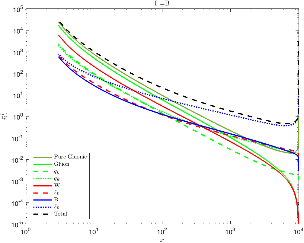
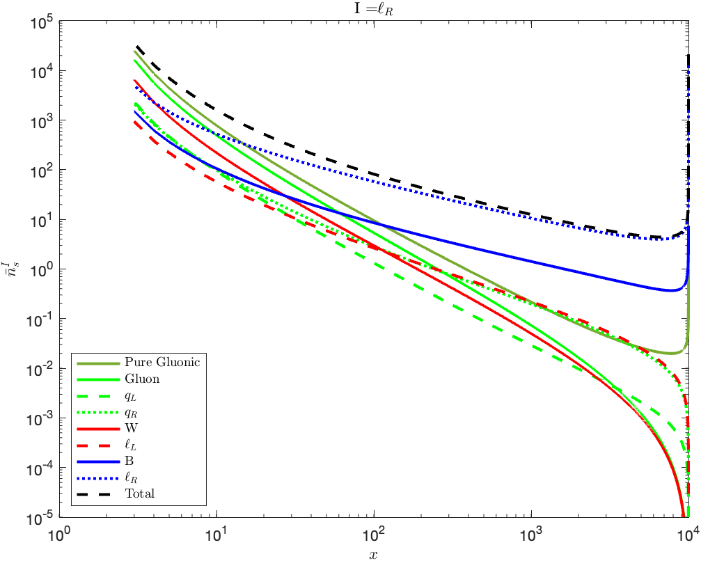
  Figure 5: Scaled number density functions $\bar{n}_{s}^{I}\left({x}\right)$ of eq.(4.1), for the various particles $s\in\mathbb{S}$, with $I=B$ (left) and $I=\ell_{R}$ (right); we use $x_{\scriptscriptstyle\rm M}=10^{4}$ for both cases.

  The right frame in figure 5 shows results for the case of $\ell_{R}$ injection. As already noted, the single splitting channel for the $SU(2)$ singlet leptons is emission of a $B$ boson, where the LPM effect partially counteracts the vacuum preference for a soft $B$. Other species of fermions are produced later in the cascade, via splittings of the $B$, hence their relative ordering can be understood as in the case of initial $B$ injection. The other gauge bosons can at the earliest be produced in tertiary splitting reactions, e.g. $\ell_{R}\rightarrow B\rightarrow q_{L}\rightarrow g,\,W$, hence their spectra fall off fastest as $x\rightarrow x_{\scriptscriptstyle\rm M}$.

  Despite the discussed relatively later production in the splitting cascade, strongly interacting particles eventually dominate the non–thermal cascade. For original injection of $B$ bosons, where quarks and gluons are already among the products of primary and secondary splitting reactions, this occurs for $x/x_{\scriptscriptstyle\rm M}<10^{-2}$, while for original injection of $\ell_{R}$ leptons this species dominates the total flux as long as $x/x_{\scriptscriptstyle\rm M}>10^{-3}$. Note that at $x\ll x_{\scriptscriptstyle\rm M}$ the gluon number density approaches that of the pure gluon solution as advertised.

  While the eventual dominance of particles with the strongest interactions in the cascade seems intuitively reasonable, within our formalism the reason for this dominance is actually rather subtle, relying on the interplay of various charge assignments, couplings, and group factors. Let us compare, as an example of this interplay, the spectrum of gluons to that of $W$ bosons. In fig. 5 these spectra are very similar as $x\rightarrow x_{\scriptscriptstyle\rm M}$. Consider the case of initial $B$ injection; the case of initial $\ell_{R}$ injection is similar, except that one more cascade step is required to produce $W$ or $g$, as noted above. Starting from an initial population of $B$ bosons, we saw above that the quark spectra at large $x$ are suppressed relative to the $\ell_{L}$ spectrum by a factor $\alpha_{W}/\alpha_{S}$, reflecting the ratio of the total splitting rates of $\ell_{L}$ and $q$; we also mentioned that the population of $q_{R}$ is an order of magnitude larger than that of $q_{L}$. Nevertheless, the LPM induced order $\alpha_{\scriptscriptstyle\rm S}/\alpha_{\scriptscriptstyle\rm W}$ larger splitting rate of $q_{L}\to W$ compared to $\ell_{L}\rightarrow W$ splittings results in both processes contributing to $W$ production parametrically at the same order in couplings in the RHS of eq.(3.12). The gluon spectrum on the other hand, receives contributions from the quark spectra, suppressed relative to $\ell_{L}$ by a factor of $\alpha_{\scriptscriptstyle\rm W}/\alpha_{\scriptscriptstyle\rm S}$; combined with the production and thermalization of gluons both being of order $\alpha_{\scriptscriptstyle\rm S}^{2}$ in couplings, this would result in a subdominant gluon spectrum at high $x$, if not for the relatively large $q_{R}$ population. These arguments show how the coincidence of the gluon and $W$ spectra at high $x$ in the case of initial $B$ injection relies on the interplay of various charge assignments, group factors, and couplings.

  In the above argument, we have assumed that the total splitting rate of non–Abelian gauge bosons is dominated by $A\to AA$ splittings. This is in fact correct for $x\gg 1$, since this rate scales like $1/y^{3/2}$ for $y\ll 1$. In contrast, the rate for $A\to FF$ only scales like $1/\sqrt{y}$, hence this contribution to the total splitting rate is suppressed by a factor $1/\sqrt{x}$ relative to that from $A\to AA$ splitting. We should emphasize that in case of the $W$, the soft gauge boson enhancement of $W\to WW$ is only partly compensated by a relative enhancement factor $\alpha_{S}/\alpha_{W}$ for the $W\to q_{L}q_{L}$ process, reflecting the larger scattering rate of quarks on the thermal background. In contrast, both the weaker coupling in the splitting matrix element and the somewhat stronger LPM suppression disfavor $q_{L}\rightarrow q_{L}W$ splitting relative to $q\rightarrow qg$ splitting. As a result, there is more flow from only weakly interacting particles to strongly interacting ones than vice versa.

  Finally, in fig. 5 and the subsequent figures we have terminated the curves at $x=3$, i.e. $p=3T$, which approximates the average energy of particles in the thermal bath. In fact, we expect the total flux to be dominated by thermal particles out to considerably larger energies, due to the (assumed) long lifetime of the matter particles whose decays trigger the cascade and the short thermalization time. Note also that the spectrum we compute becomes independent of the IR cut–off $\kappa$ only for $x\geq 10$ (as well as $x_{\scriptscriptstyle\rm M}-x\geq 10$) [36]. It is worth mentioning that this happens to be roughly the same scale at which the elastic $2\to 2$ processes get to compete with the inelastic processes, further restricting the precision of results for $x\leq 10$.

  

  

  

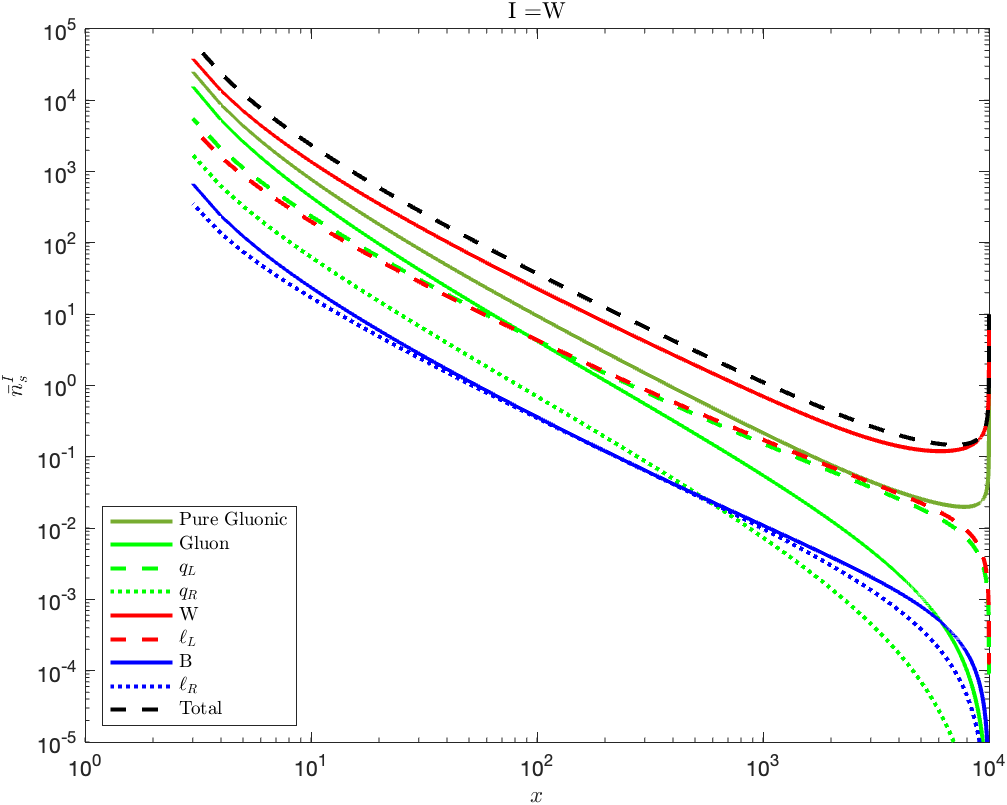
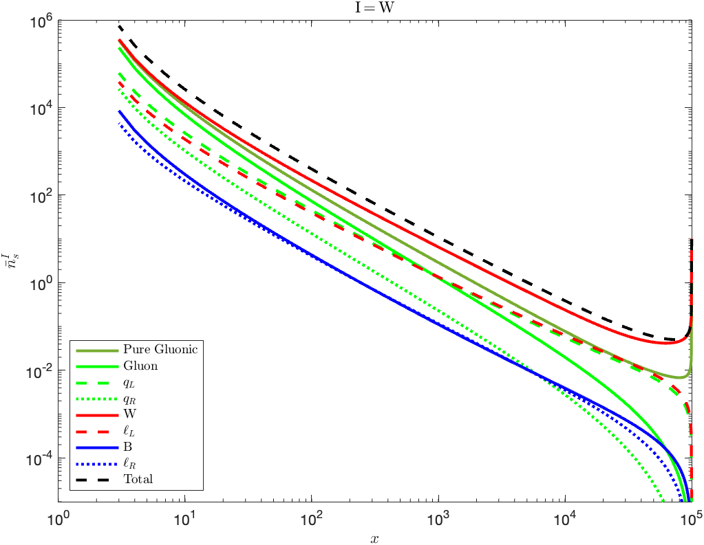
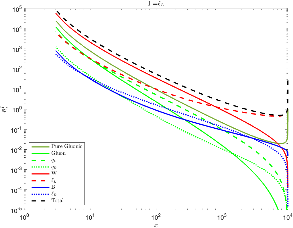
  Figure 6: Scaled number density functions $\bar{n}_{s}^{I}\left({x}\right)$ of eq.(4.1) for the various particles $s\in\mathbb{S}$, with $I=W$ (top) and $I=\ell_{L}$ (bottom); we use $x_{\scriptscriptstyle\rm M}=10^{5}$ in the top–right frame in order to show that an extra decade in $x$ allows the composition of thermalizing particles to approach domination by colored particles, in particular gluons. The top–left and bottom frames are for $x_{\scriptscriptstyle\rm M}=10^{4}$.

• $I\in\{\ell_{L},\,W\}$:
  Next, we turn to the injection of color singlet particles with $SU(2)_{L}$ interactions, which then dominate their scattering off the thermal background. Results are shown in fig. 6. The discussion following fig. 5 explains why the overall normalization at large $x$ lies in between that of the pure gluon case and the case where the injected particles have only $U(1)_{Y}$ interactions. Moreover, we again see that at sufficiently small $x$ colored particles begin to dominate the non–thermal cascade.

  In detail, let us first consider the case of $W$ injection (top frames). We see that the flow towards the dominance of colored states is considerably slower than for the injection of $B$ bosons. This is partly because $SU(2)_{L}$ interactions in the SM are stronger than $U(1)_{Y}$ interactions and thus closer to the strong $SU(3)_{C}$ processes, but mostly because $SU(2)_{L}$ is a non–Abelian group allowing $A\rightarrow AA$ splittings; eqs.(2.17) show that the corresponding rate is enhanced by a factor $1/[y(1-y)]$ relative to that of $A\rightarrow FF$ splittings. Therefore the original $W$ bosons strongly prefer to emit additional soft $W$ bosons, rather than splitting into quark antiquark pairs which leads to a transition to colored particles. An analogous argument also shows why the flux of non–Abelian gauge bosons eventually overtakes that of $SU(2)_{L}-$charged fermions in the case of fermion injection: only the relatively inefficient $A\rightarrow FF$ splittings increase the number of fermions in the cascade, while each $A\rightarrow AA$ and $F\rightarrow AF$ splitting increases the number of gauge bosons; the rate for the latter is still enhanced by a factor $1/y$ relative to that for $A\rightarrow FF$.

  Due to the high efficiency of $W\rightarrow WW$ splitting, for $x_{\scriptscriptstyle\rm M}=10^{4}$ (top left) the gluon flux eventually catches up with, but does not overtake, the $W$ flux. However, extending the cascade by another decade by setting $x_{\scriptscriptstyle\rm M}=10^{5}$ (top right), gluons do indeed begin to dominate at the smallest values of $x$ shown.

  The small rate of $A\rightarrow FF$ splittings relative to non–Abelian $A\rightarrow AA$ also explains why the spectra of $SU(2)$ doublet fermions, which can in principle be produced in the first splitting of the original $W$ bosons, do not spike as $x\rightarrow x_{\scriptscriptstyle\rm M}$, in contrast to the fermion spectra in the left frame of fig. 5. Here the enhancement of $q_{L}$ production compared to splittings to $\ell_{L}$, by the color factor and the LPM induced relative factor of $\alpha_{\rm s}/\alpha_{\scriptscriptstyle\rm W}$ is largely canceled by the more efficient thermalization of quarks relative to $\ell_{L}$, leading to very similar normalization of these two spectra at large $x$. At much smaller $x$, the flux of $q_{L}$ (and, for $x_{\scriptscriptstyle\rm M}\gg 10^{4}$ eventually $q_{R}$) overtakes that of $\ell_{L}$, due to quark production in (tertiary) gluon splitting. Since all $SU(2)$ singlet fermions require at least three splitting reactions to be produced, e.g. $W\rightarrow\ell_{L}\rightarrow B\rightarrow\ell_{R}$, their spectra fall of very quickly as $x\rightarrow x_{\scriptscriptstyle\rm M}$.

  The bottom frame of fig. 6 shows the non–thermal spectra that result from the injection of $SU(2)$ doublet leptons $\ell_{L}$. Here the two possible primary splittings are the emission of a $W$ or $B$ boson. Since the corresponding differential rates scale like $1/[y^{3/2}\sqrt{1-y}]$ and $1/\sqrt{y(1-y)}$, respectively (see eq.(2.17b)), the emitted gauge bosons are predominantly soft, i.e. their spectra do not spike as $x\rightarrow x_{\scriptscriptstyle\rm M}$; clearly soft gauge bosons are even more strongly favored in case of $W$ emission, which explains the difference between the shapes of the $W$ and $B$ spectra as $x\to x_{\scriptscriptstyle\rm M}$. On the other hand, $SU(2)$ singlet (right–chiral) fermions can now already be produced in the second step of their cascade, so their spectra at large $x$ lie well above those shown in the top frames. In contrast, gluons now require at least three splitting reactions to be produced; this, and their very short thermalization time, implies that they have by far the smallest spectrum as $x\rightarrow x_{\scriptscriptstyle\rm M}$. This also explains why their flux remains below the flux of $W$ bosons even for the smallest $x$ shown; however, our earlier arguments show that gluons will eventually dominate the cascade if $x_{\scriptscriptstyle\rm M}\gg 10^{4}$.

  We finally note that despite similar interactions the shape of the $W$ spectrum in the $W$ injection scenario (top frames) differs a bit from that of the $\ell_{L}$ spectrum in the bottom frame. Note that the dominant rate for $A\rightarrow AA$ splittings is enhanced by a factor $1/(1-y)$ relative to that for $F\rightarrow AF$ splittings. This favors the emission of relatively harder $W$ bosons from an initial $W$, speeding up the loss of very energetic $W$s in the cascade. This loss is further enhanced by $A\rightarrow FF$ splittings which, while rare, reduce the number of gauge bosons in the cascade. In contrast, emission off fermions favors very soft gauge bosons, leading to smaller energy loss; note also that no splitting process can reduce the number of fermions in the cascade. These two effects combine to produce a quite pronounced minimum in the $W$ spectrum for the case of $W$ injection, at $x\sim x_{\scriptscriptstyle\rm M}/2$, whereas the $\ell_{L}$ spectrum for the case of $\ell_{L}$ injection reaches its minimum closer to $x_{\scriptscriptstyle\rm M}$, and rises more slowly for smaller $x$. The $x$ dependence of the denominator in eq.(3.12) also plays a role in determining the shape of the spectra near their minimum.

  

  

  

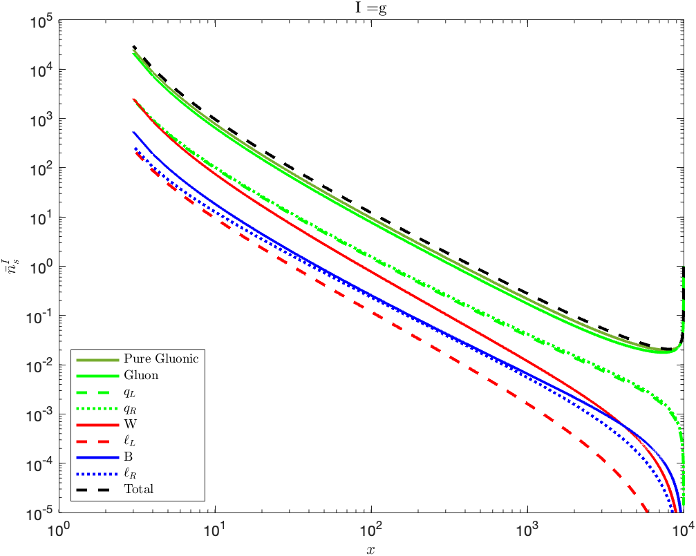
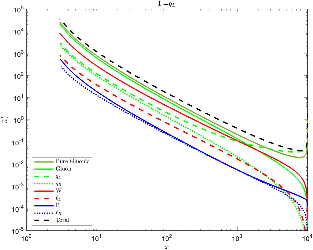
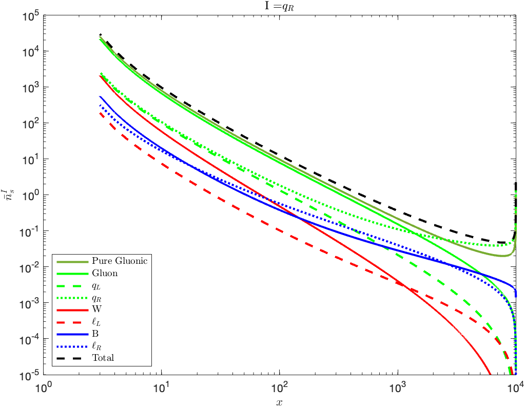
  Figure 7: The scaled number density functions $\bar{n}_{s}^{I}\left({x}\right)$ of eq.(4.1) for the various particles $s\in\mathbb{S}$, with $I=g$ (top Left), $I=q_{L}$ (top right) and $I=q_{R}$ (bottom); we use $x_{\scriptscriptstyle\rm M}=10^{4}$ for all three cases.

• $I\in\{g,\,q_{L},\,q_{R}\}$
  Finally, let us discuss the cases where the injected particles are charged under $SU(3)_{C}$. The resulting spectra are shown in fig. 7 for injected gluons (top left), $SU(2)$ doublet quarks (top right), and $SU(2)$ singlet quarks (bottom).

  Not surprisingly, in all three cases colored particles remain the dominant species in the spectrum, with the gluons eventually ending up on top. If gluons are the injected particles, their spectrum is quite close to that of a pure gluon cascade for all $x$, with a slight reduction of the normalization due to the loss of gluons from splitting into quarks. This splitting does not distinguish between left– and right–chiral quarks, whose spectra are therefore very similar. The latter two almost identical spectra of $q_{L}$ and $q_{R}$ will further source electroweak gauge bosons and leptons, appearing first in the second and third step of the cascade, respectively. Radiations of $B$ from $q_{R}$ will favor harder $B$s as discussed above, resulting in a sharper rise of the $B$ spectrum at $x\to x_{\scriptscriptstyle\rm M}$ as compared to that of $W$s. The $W$ spectrum overtakes that of the $B$ at lower $x$ despite a larger thermalization rate as a result of dominant $W\to WW$ splittings; the $B$s on the other hand disappear after each splitting. As before, the $\ell_{R}$ population is exclusively sourced by, and therefore tracks, that of the $B$, with the former winning gradually as a result of conserved $\ell_{R}$ in splittings. With the $W$ predominantly sourcing the $W$ and $q_{L}$ spectra, only a small fraction of all $W$ bosons splits into $\ell_{L}$ pairs; this, together with having a larger thermalization rate compared to that of $\ell_{R}$ make the $\ell_{L}$ spectrum subdominant.

  If quarks are injected, gluons dominate the cascade only for $x<x_{\scriptscriptstyle\rm M}/10$, but then the gluon spectrum again quickly approaches that of a pure gluon cascade. Moreover, if $q_{L}$ are injected, $q_{R}$ production requires at least two splitting reactions, and vice versa; as a result, the $q_{L}$ and $q_{R}$ spectra are very different at large $x$, and converge only for $x\leq 10^{-2}x_{\scriptscriptstyle\rm M}$.

  The chirality of the injected quark is further reflected in the large gap between the $W$ and $B$ populations in the two cases: if $q_{L}$ quarks are injected, all electroweak gauge bosons can be produced in the first step of the cascade, albeit with significantly smaller rates than gluons; in contrast, for $q_{R}$ injection, $W$ bosons can only be produced in the third step, e.g. $q_{R}\rightarrow g\rightarrow q_{L}\rightarrow W$. As a result, in the bottom frame $W$ bosons have the smallest flux at large $x$, and the flux of $SU(2)$ doublet leptons, which (due to their smaller hypercharge) are predominantly produced in the splitting of $W$ bosons, remain below that of $SU(2)$ singlet leptons over the entire range of $x$ shown; note once again that the latter spectrum is also enhanced by the smaller thermalization rate of $\ell_{R}$.

  Finally, as already discussed in the context of fig. 6 the shape of the spectrum of the injected particle at large $x$ depends to some extent on whether it is a fermion of gauge boson species.

Figures 5, 6 and 7 show that for $x$ not much below $x_{\scriptscriptstyle\rm M}$ both the shape and the normalization of the spectra quite strongly depend on the identity of the injected particle, i.e. on the branching ratios of the long–lived matter particles. However, these differences diminish as $x$ becomes smaller; hence with increasing $x_{\scriptscriptstyle\rm M}$ a larger and larger part of the spectrum will be largely independent of the high–scale $Br_{\scriptscriptstyle\rm I}$ parameters.

4.2 The role of $x_{\scriptscriptstyle\rm M}$ and scaling behavior

In this subsection we quantitatively analyze the role of $x_{\scriptscriptstyle\rm M}$ in the normalization and shape of the spectra of non–thermal particles. We saw in eq.(3.9) that for a pure gluon cascade the normalized spectrum is essentially given by $1/\sqrt{x_{\scriptscriptstyle\rm M}}$ times the function (3.10) which only depends on the ratio $x/x_{\scriptscriptstyle\rm M}$, with minor corrections. If this holds also for the multi–species cascade we are analyzing here, the ratios

$$r_{s}^{\scriptscriptstyle\rm I}\left({x,x_{\scriptscriptstyle\rm M}}\right)=\frac{\bar{n}_{s}^{I}\left({x,x_{\scriptscriptstyle\rm M}}\right)}{\bar{n}_{gg}^{g}\left({x,x_{\scriptscriptstyle\rm M}}\right)}$$ (4.2)

should to good approximation only depend on the ratio $x/x_{\scriptscriptstyle\rm M}$; here $\bar{n}_{gg}^{g}$ denotes the pure gluon solution of (3.8), using the full splitting rate of eq.(2.17a).

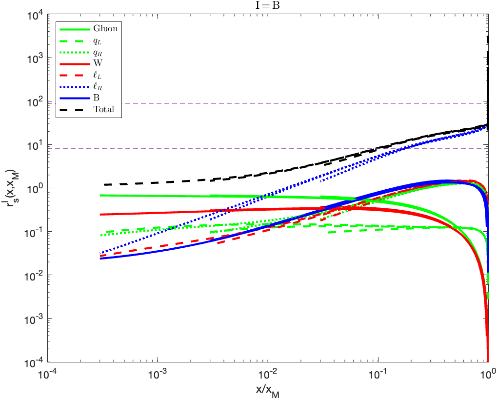
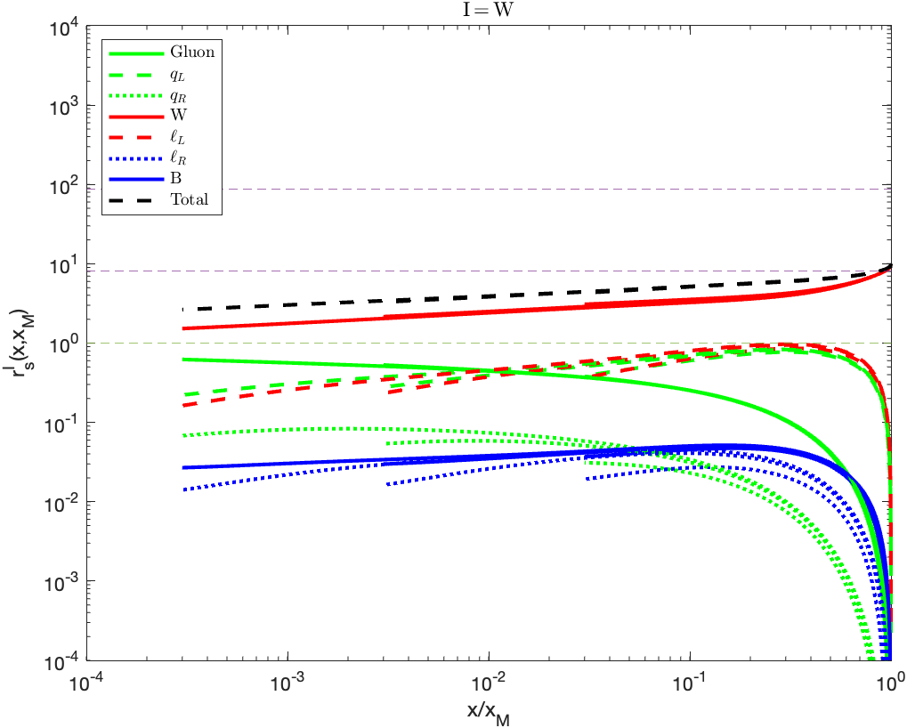
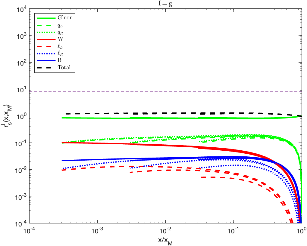
Figure 8: Ratios $r_{s}^{I}\left({x,x_{\scriptscriptstyle\rm M}}\right)$ of eq.(4.2), for three initial populations: $I=B$ (top left), $W$ (top right), and $g$ (bottom). Results for $x_{\scriptscriptstyle\rm M}=10^{2},\,10^{3},\,10^{4}$ are overlaid. The dark green horizontal dashed line marks $r=1$, corresponding to a pure gluon cascade. The two purple dashed lines show the ratios $\frac{\Gamma^{\rm split}_{\scriptscriptstyle\rm LPM}\left({g,x_{\scriptscriptstyle\rm M}}\right)}{\Gamma^{\rm split}_{\scriptscriptstyle\rm LPM}\left({W,x_{\scriptscriptstyle\rm M}}\right)}$, and $\frac{\Gamma^{\rm split}_{\scriptscriptstyle\rm LPM}\left({g,x_{\scriptscriptstyle\rm M}}\right)}{\Gamma^{\rm split}_{\scriptscriptstyle\rm LPM}\left({B,x_{\scriptscriptstyle\rm M}}\right)}$, see eq.(3.14), which determine the normalizations of the spectra of injected $W$ and $B$ bosons, respectively, for $x\rightarrow x_{\scriptscriptstyle\rm M}$.

Some results are shown in fig. 8. Here we focus on scenarios where the injected particles are gauge bosons, $I=g,\,W,\,$ and $B$, and overlaid curves for three values of $x_{\scriptscriptstyle\rm M}=10^{2},\,10^{3},\,$ and $10^{4}$. We see that the rescaled spectra of gauge bosons indeed to very good approximation only depend on $x/x_{\scriptscriptstyle\rm M}$. We saw in the discussion of fig. 5 that the evolution equations are quite similar for gluons and for $W$ bosons; it is therefore not surprising that the rescaled $W$ spectra $r_{W}$ don’t show a strong dependence on $x_{\scriptscriptstyle\rm M}$, and become quite flat at $x\ll x_{\scriptscriptstyle\rm M}$. The evolution equation for Abelian $B$ bosons is quite different, however, due to the absence of $B\rightarrow BB$ splitting and the strong LPM suppression of $F\rightarrow BF$ splitting. It is therefore not surprising that $r_{B}$ can have quite a different shape than $r_{W}$; the fact that $r_{B}$ to very good approximation depends on $x_{\scriptscriptstyle\rm M}$ only via the ratio $x/x_{\scriptscriptstyle\rm M}$ appears to be “accidental”.

In our results, the rescaled fermion spectra do show some residual dependence on $x_{\scriptscriptstyle\rm M}$. This is especially pronounced for $r_{\ell_{R}}$; right–chiral leptons can lose energy only via emission of $B$ bosons. Recall that the corresponding differential splitting rate only scales like $1/\sqrt{y}$ for small $y$, while all rates for emitting a non–Abelian gauge boson scale like $1/y^{3/2}$ in that limit. $\ell_{R}$ therefore typically emits more energetic gauge bosons, leading to a significantly shorter cascade and hence a stronger dependence on the boundary conditions.

The other rescaled fermion spectra explicitly depend on $x_{\scriptscriptstyle\rm M}$ mostly at relatively small $x$. This may reflect the effect of $A\rightarrow FF$ splitting on the total splitting rate of $A$ which, as we saw above, becomes relatively more important at smaller $x$. The same effect also explains why the explicit $x_{\scriptscriptstyle\rm M}$ dependence is somewhat stronger for left–chiral leptons than for quarks; we saw in the discussion of fig. 5 that $A\rightarrow FF$ splitting is more important for $A=W$ than for $A=g$.

Figure 8 also illustrates the flow towards a non–thermal spectrum dominated by gluons and quarks, irrespective of the initial injection. In particular, in the case of gluon injection, the ratio functions settle quickly into their asymptotic values, so that the particle ratios depend only weakly on $x$ for $x\leq 0.1x_{\scriptscriptstyle\rm M}$. At least for this scenario, and for the given values of the gauge couplings, one should therefore be able to predict the various ratio functions for $x_{\scriptscriptstyle\rm M}>10^{4}$ quite accurately by extrapolating the numerical results of the bottom frame of fig. 8, without the need for new numerical solutions of eqs.(3.12); recall that the gauge couplings do depend weakly on $T$, and hence on $x_{\scriptscriptstyle\rm M}$ for fixed $M$. Not surprisingly, if the injected particle is a color singlet, a longer cascade is required before strongly interacting particles dominate.

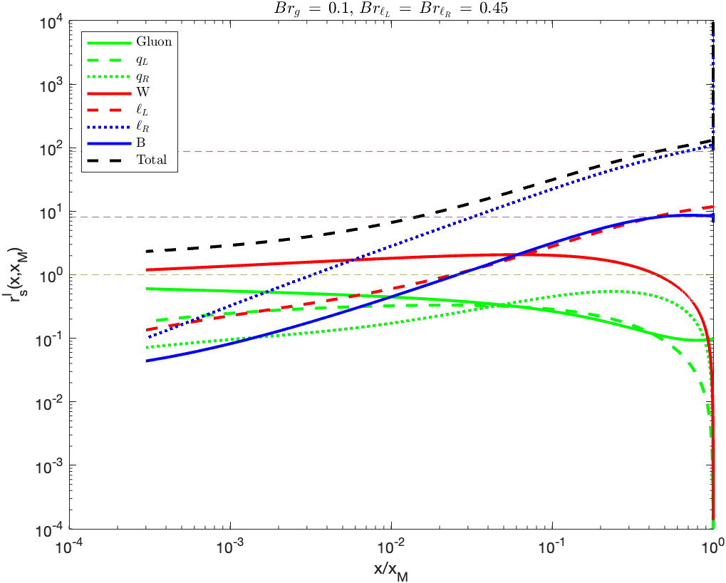
Figure 9: Ratios $r_{s}\left({x,x_{\scriptscriptstyle\rm M}}\right)$ for a scenario where several species are injected, with branching ratios $Br_{g}=0.1,\,Br_{\ell_{L}}=Br_{\ell_{R}}=0.45$, with $x_{\scriptscriptstyle\rm M}=10^{4}$. The dashed horizontal lines correspond to an initial $W$ and $B$ injection as explained in fig. 8.

Finally, once all $\bar{n}_{s}^{I}\left({x}\right)$ have been computed one can use eq.(4.1) to deduce the spectrum of non–thermal particles for any given set of branching ratios $Br_{I}$. One such example is shown in fig. 9, where we assumed $Br_{g}=0.1,\,Br_{\ell_{L}}=Br_{\ell_{R}}=0.45$ with $x_{\scriptscriptstyle\rm M}=10^{4}$; we checked explicitly that a direct numerical solution of eqs.(3.12) gives the same result. We see that the spectrum remains dominated by $\ell_{R}$ for most of the range of $x$; this reflects the very large normalization of the $\ell_{R}$ spectrum, as discussed previously for fig. 5.

5 Application: semi-thermal production of heavy dark matter

As an example of the application of our results, we briefly discuss the production of heavy particles $\chi$ via annihilation reactions involving one non–thermal particle and one particle from the thermal bath. For definiteness, we will assume that the long–lived particles, with mass $M$ and decay width $\Gamma_{\scriptscriptstyle\rm M}$, whose decays were ultimately responsible for the spectra of non–thermal particles, dominates the energy density of the universe prior to its decay. Moreover, we will focus on the case where the lifetime of the produced particles is much larger than $1/\Gamma_{\rm M}$, so that we can treat them as stable; this is certainly true if we are interested in the production of dark matter.

The long–lived very massive particles dominated the energy density as long as the temperature is above the reheating temperature, which is given by

$$T_{\scriptscriptstyle\rm RH}\sim\sqrt{\Gamma_{\scriptscriptstyle\rm M}M_{\scriptscriptstyle\rm Pl}}\,,$$ (5.1)

where $M_{\scriptscriptstyle\rm Pl}$ is the reduced Planck mass. If $m_{\chi}\mbox{~{}{\raisebox{1.72218pt}{$<$}} {\raisebox{-2.58334pt}{$\sim$}}~{}}T_{\scriptscriptstyle\rm RH}$, total $\chi$ pair production through renormalizable interactions will be dominated by reactions only involving thermalized particles, so the resulting $\chi$ density will be insensitive to the details of the spectrum of nonthermal particles. On the other hand, if $m_{\chi}\gg 20T_{\scriptscriptstyle\rm RH}$, thermal production of $\chi$ particles with roughly weak–strength cross sections (e.g. the well–known WIMPs [59]) will effectively cease at temperature $T_{\scriptscriptstyle\rm P}\sim\mathcal{O}\left({0.05m_{\chi}}\right)>T_{\scriptscriptstyle\rm RH}$; a possible thermal contribution to the $\chi$ density will then be diluted by the entropy production between $T_{\scriptscriptstyle\rm P}$ and $T_{\scriptscriptstyle\rm RH}$. In this case the final $\chi$ density may well be dominated by non–thermal (or semi–thermal) processes of the kind

$$s\,s^{\prime}\longrightarrow\chi\,\chi\,,$$ (5.2)

where $s^{\prime}$ denotes a particle from the thermal bath but $s$ is taken from the spectrum of non–thermal particles, with momentum $p_{s}\gg T$. We denote the corresponding production cross section by $\sigma_{\chi}^{\scriptscriptstyle\rm ST}$. The $\chi$ number density $n_{\chi}$ then obeys the equation

$$\frac{dn_{\chi}^{\scriptscriptstyle\rm ST}\left({T}\right)}{dt}+3Hn_{\chi}^{\scriptscriptstyle\rm ST} = \sum_{s,\,s^{\prime}}\int n_{s^{\prime}}\left({T}\right)\langle\sigma_{\chi}^{\scriptscriptstyle\rm ST}v\rangle\left({p,T}\right)\tilde{n}_{s}\left({p,T}\right)dp$$ (5.3)

$$= \sum_{s,\,s^{\prime}}\int n_{s^{\prime}}\left({T}\right)\langle\sigma_{\chi}^{\scriptscriptstyle\rm ST}v\rangle\left({p,T}\right)r_{s}\left({p,T}\right)\tilde{n}_{gg}^{g}\left({p,T}\right)dp\,.$$

Here $n_{s^{\prime}}\left({T}\right)=c_{s^{\prime}}\zeta(3)g_{s^{\prime}}T^{3}/\pi^{2}$ with $c_{s^{\prime}}=1\ (3/4)$ for bosonic (fermionic) $s^{\prime}$ is the thermal number density of the species $s^{\prime}$ with $g_{s^{\prime}}$ degrees of freedom, $\langle\sigma_{\chi}^{\scriptscriptstyle\rm ST}v\rangle$ denotes the thermal average of the production cross section, and we have used eq.(3.13) to write $\tilde{n}_{s}\left({p,T}\right)$ in terms of the pure gluon solution of eq.(3.8). In eq.(5.3) we have assumed that $n_{\chi}$ remains so small that $\chi$ annihilation processes are irrelevant. While analytic approximations and numerical solutions for the pure gauge solution have previously been used to estimate the $\chi$ number density, our knowledge of the ratios $r_{s}$ allows for a much more precise calculation for the production rate of the process (5.2).

Of course, $\chi$ pair production is only possible if the center–of–mass energy exceeds $2m_{\chi}$. Since the average energy of a particle in the thermal bath is around $3T$ and the spectrum of non–thermal particles quickly increases with decreasing momentum, the dominant contribution to the integral in eq.(5.3) typically comes from $p\sim m_{\chi}^{2}/T$. Together with the fact that $n_{s^{\prime}}\propto T^{3}$ in eq.(5.3), this implies that the $\chi$ production rate quickly increases with increasing $T$. However, the entropy dilution factor [36] $(T_{\rm RH}/T)^{5}$ implies that nevertheless the biggest contribution to the final $\chi$ density often comes from temperature $T\simeq T_{\rm RH}$, unless $m_{\chi}^{2}>T_{\rm RH}M$. If $m_{\chi}^{2}\ll T_{\rm RH}M$ the semi–thermal production rate will be dominated by particles with energy $p\ll M$, whose spectrum is less dependent on the decay branching ratios of our heavy matter particles. In contrast, for $m_{\chi}^{2}\mbox{~{}{\raisebox{1.72218pt}{$>$}} {\raisebox{-2.58334pt}{$\sim$}}~{}}T_{\rm RH}M$, very energetic particles with $p\sim M/2$ will make sizable or even dominant contributions; their spectra do strongly depend on the initial branching ratios. As long as $m_{\chi}^{2}<T_{\rm max}M$, where $T_{\rm max}$ is the maximal temperature of the early matter dominated epoch, most $\chi$ particles will be produced at temperature $T\sim m_{\chi}^{2}/M$.

Finally, the production of very massive particles, with $m_{\chi}^{2}\mbox{~{}{\raisebox{1.72218pt}{$>$}} {\raisebox{-2.58334pt}{$\sim$}}~{}}T_{\rm max}M$, will be dominated by purely non–thermal processes, where both initial particles in the reaction (5.2) are non–thermal [12, 30, 36]. The distinction between the various species is in that case of even greater importance as now the product of ratios $r_{s}r_{s^{\prime}}$ appears. We leave a more careful study of dark matter production from different phases of a generic matter domination era for a future work.

6 Summary and discussion

Cosmological histories including an early matter domination epoch, where the energy density of the universe is dominated by a long–lived matter component of mass $M$ and decay width $\Gamma_{\scriptscriptstyle\rm M}$, are well motivated and have been studied in many recent publications. The inclusion of such a period has been shown to potentially affect various aspects of cosmology, including the production of dark matter or the baryon asymmetry. Since we know that the universe was dominated by the SM radiation bath at the latest at the onset of BBN, any matter component should decay and eventually (predominantly) thermalize into the thermal bath.

The thermalization procedure entails the splitting of initial decay products of energy $p_{i}\gg T$ into $\mathcal{O}\left({p_{i}/T}\right)$ particles of energy $\mathcal{O}\left({T}\right)$, and has been studied in the literature both in cosmological contexts and in the context of heavy ion collisions. So long as the out of equilibrium particles are gauge charged, the dominant process of thermalization is known to be the $1\to 2$ near collinear splittings of the energetic particles made possible via soft $t-$channel interactions with the thermal bath, mediated by gauge bosons with thermal mass $\mathcal{O}\left({gT}\right)$, $g$ being the relevant gauge coupling. The collinearity of the splitting then calls for a careful inclusion of the LPM effect resulting from consecutive interactions of the particles with the plasma during the formation time of the splitting process. The LPM suppressed rate of pure–gauge splittings $g\to gg$ had already been studied analytically and numerically in the literature; these studies are motivated by the fact that the QCD sector, and in particular gluons, can be expected to dominate the spectrum of nonthermal particles, at least for momenta $p\ll p_{i}$.

In this study, we extend the previous works by including the full set of chiral SM fermions and gauge bosons in the splitting cascade of an initial population of energetic particles of energy $p_{i}=M/2$. The functions describing the emission of a gauge boson all have similar functional form, but can have different coupling strengths, flavor multiplicity factors, and numerical LPM suppression factors; evidently these processes increase the number of gauge bosons. In contrast, the splitting of a gauge boson into an $f\bar{f}$ pair is suppressed by a factor $p_{d}/p_{p}$, where $p_{d}$ and $p_{p}$ denote the momentum of the softer daughter and parent particle, respectively; it increases the number of fermions, but reduces the number of gauge bosons. Note also that this is the only splitting process available to Abelian gauge bosons.

We use the explicitly calculated results for LPM suppressed splitting rates corresponding to an $SU(N)$ gauge group from the literature, and use physical arguments to deduce the rate for processes involving species charged under different gauge groups, see eqs.(2.16) to (2.19). The resulting Boltzmann equations can be written in terms of the dimensionless ratio $x=p/T$, see eq.(3.12); in this form the equations depend only on $x_{\scriptscriptstyle\rm M}=M/2T$ rather than on $M$ and $T$ separately. Of course, the decay branching ratios of the matter particles into the various SM species are also important, but due to the linearity of the problem, we only need to consider the limiting cases where decay into a single species dominates. The corresponding numerical results are shown in figures 5 to 7.

We find that spectra of individual species can have order of magnitude deviations from that of the pure–gluon solution over several decades of momentum, i.e. for $1\mbox{~{}{\raisebox{1.72218pt}{$<$}} {\raisebox{-2.58334pt}{$\sim$}}~{}}x/x_{\scriptscriptstyle\rm M}\mbox{~{}{\raisebox{1.72218pt}{$<$}} {\raisebox{-2.58334pt}{$\sim$}}~{}}10^{3}$. We treat the fermion chiralities separately, since only left–chiral fermions (and right–chiral antifermions) have $SU(2)$ interaction. In scenarios with an initial chiral asymmetry in the matter decay products, it also persists for several decades in $x$. On the other hand, an approximate scale invariant behavior is observed for the ratios of the various species (4.2), which for $x\ll x_{\scriptscriptstyle\rm M}$ asymptotically approach unique solutions independent of the branching ratios.

Our treatment should suffice for many practical purposes, greatly improving the precision of the calculation of cosmological processes involving non–thermal particles. The validity of the results is however limited by the approximations we made. For example, in writing the Boltzmann equations (3.12), we disregard the role of hard $2\to 2$ processes. This should be a good approximation so long as $x\gg 1$, but the low$-x$ tail of our result could be affected. On the other hand, these results for the ratios of spectra, together with the pure gluon solution, should serve as a good approximation for $x\gg 1$ regions even for cases with $x_{\scriptscriptstyle\rm M}\gg 10^{4}$ as we argued in section 4. Recall also that the total flux of particles with momentum $p\mbox{~{}{\raisebox{1.72218pt}{$<$}} {\raisebox{-2.58334pt}{$\sim$}}~{}}10T$ will in any case be dominated by the thermal component.

Moreover, we did not allow for the production of scalar particles in the cascade. In section 2.3 we argued that we may safely leave out the SM Higgs doublet in our analysis, but this may be different in models with extended Higgs sectors (with more degrees of freedom, and often also enhanced couplings to some fermions). Scalars, and Majorana gauginos, will certainly be important if one wishes to analyze a supersymmetric cascade. Results for medium induced scalar–scalar–gauge boson splittings have been published in the literature [47]; these would need to be augmented with splitting functions involving Yukawa interactions.

References

- [1] E. W. Kolb and M. S. Turner, “The Early Universe,” Front. Phys.69 (1990).
- [2] R. Allahverdi, R. Brandenberger, F. Y. Cyr-Racine and A. Mazumdar, “Reheating in Inflationary Cosmology: Theory and Applications,” Ann. Rev. Nucl. Part. Sci. 60 (2010), 27, doi:10.1146/annurev.nucl.012809.104511 [arXiv:1001.2600 [hep-th]].
- [3] G. Kane, K. Sinha and S. Watson, “Cosmological Moduli and the Post-Inflationary Universe: A Critical Review,” Int. J. Mod. Phys. D 24 (2015) no.08, 1530022, doi:10.1142/S0218271815300220 [arXiv:1502.07746 [hep-th]].
- [4] R. Allahverdi et al., “The First Three Seconds: a Review of Possible Expansion Histories of the Early Universe,” doi:10.21105/astro.2006.16182 [arXiv:2006.16182 [astro-ph.CO]].
- [5] G. F. Giudice, E. W. Kolb and A. Riotto, “Largest temperature of the radiation era and its cosmological implications,” Phys. Rev. D 64 (2001), 023508 doi:10.1103/PhysRevD.64.023508 [arXiv:hep-ph/0005123 [hep-ph]].
- [6] S. Hannestad, “What is the lowest possible reheating temperature?”, Phys. Rev. D 70 (2004), 043506 doi:10.1103/PhysRevD.70.043506 [arXiv:astro-ph/0403291 [astro-ph]].
- [7] J. T. Giblin, G. Kane, E. Nesbit, S. Watson and Y. Zhao, “Was the Universe Actually Radiation Dominated Prior to Nucleosynthesis?,” Phys. Rev. D 96 (2017) no.4, 043525 doi:10.1103/PhysRevD.96.043525 [arXiv:1706.08536 [hep-th]].
- [8] A. Berlin, D. Hooper and G. Krnjaic, “PeV-Scale Dark Matter as a Thermal Relic of a Decoupled Sector,” Phys. Lett. B 760 (2016), 106-111 doi:10.1016/j.physletb.2016.06.037 [arXiv:1602.08490 [hep-ph]].
- [9] A. Berlin, D. Hooper and G. Krnjaic, “Thermal Dark Matter From A Highly Decoupled Sector,” Phys. Rev. D 94 (2016) no.9, 095019 doi:10.1103/PhysRevD.94.095019 [arXiv:1609.02555 [hep-ph]].
- [10] D. J. H. Chung, E. W. Kolb and A. Riotto, “Production of massive particles during reheating,” Phys. Rev. D 60 (1999), 063504, doi:10.1103/PhysRevD.60.063504 [arXiv:hep-ph/9809453 [hep-ph]].
- [11] R. Allahverdi and M. Drees, “Production of massive stable particles in inflaton decay,” Phys. Rev. Lett. 89 (2002), 091302, doi:10.1103/PhysRevLett.89.091302 [arXiv:hep-ph/0203118 [hep-ph]].
- [12] R. Allahverdi and M. Drees, “Thermalization after inflation and production of massive stable particles,” Phys. Rev. D 66 (2002) 063513 doi:10.1103/PhysRevD.66.063513 [hep-ph/0205246].
- [13] G. B. Gelmini and P. Gondolo, “Neutralino with the right cold dark matter abundance in (almost) any supersymmetric model”, Phys. Rev. D 74 (2006) 023510 doi:10.1103/PhysRevD.74.023510 [hep-ph/0602230].
- [14] B. S. Acharya, P. Kumar, K. Bobkov, G. Kane, J. Shao and S. Watson, “Non-thermal Dark Matter and the Moduli Problem in String Frameworks”, JHEP 06 (2008), 064, doi:10.1088/1126-6708/2008/06/064 [arXiv:0804.0863 [hep-ph]].
- [15] G. Kane, J. Shao, S. Watson and H. B. Yu, “The Baryon-Dark Matter Ratio Via Moduli Decay After Affleck-Dine Baryogenesis”, JCAP 11 (2011), 012, doi:10.1088/1475-7516/2011/11/012 [arXiv:1108.5178 [hep-ph]].
- [16] J. Hasenkamp and J. Kersten, “Dark radiation from particle decay: cosmological constraints and opportunities”, JCAP 08 (2013), 024, doi:10.1088/1475-7516/2013/08/024 [arXiv:1212.4160 [hep-ph]].
- [17] Y. Kurata and N. Maekawa, “Averaged Number of the Lightest Supersymmetric Particles in Decay of Superheavy Particle with Long Lifetime”, Prog. Theor. Phys. 127 (2012) 657, doi:10.1143/PTP.127.657 [arXiv:1201.3696 [hep-ph]].
- [18] K. Harigaya, M. Kawasaki, K. Mukaida and M. Yamada, “Dark Matter Production in Late Time Reheating”, Phys. Rev. D 89 (2014) no.8, 083532, doi:10.1103/PhysRevD.89.083532 [arXiv:1402.2846 [hep-ph]].
- [19] K. Ishiwata, “Axino Dark Matter in Moduli-induced Baryogenesis”, JHEP 09 (2014), 122, doi:10.1007/JHEP09(2014)122 [arXiv:1407.1827 [hep-ph]].
- [20] G. L. Kane, P. Kumar, B. D. Nelson and B. Zheng, “Dark matter production mechanisms with a nonthermal cosmological history: A classification”, Phys. Rev. D 93 (2016) no.6, 063527 doi:10.1103/PhysRevD.93.063527 [arXiv:1502.05406 [hep-ph]].
- [21] R. T. Co, F. D’Eramo, L. J. Hall and D. Pappadopulo, “Freeze-In Dark Matter with Displaced Signatures at Colliders”, JCAP 1512 (2015) no.12, 024, doi:10.1088/1475-7516/2015/12/024 [arXiv:1506.07532 [hep-ph]].
- [22] M. Dhuria, C. Hati and U. Sarkar, “Moduli induced cogenesis of baryon asymmetry and dark matter”, Phys. Lett. B 756 (2016), 376-383 doi:10.1016/j.physletb.2016.03.018 [arXiv:1508.04144 [hep-ph]].
- [23] S. Hamdan and J. Unwin, “Dark Matter Freeze-out During Matter Domination”, Mod. Phys. Lett. A 33 (2018) no.29, 1850181, doi:10.1142/S021773231850181X [arXiv:1710.03758 [hep-ph]].
- [24] H. Kim, J. P. Hong and C. S. Shin, “A map of the non-thermal WIMP,” Phys. Lett. B 768 (2017) 292 doi:10.1016/j.physletb.2017.03.005 [arXiv:1611.02287 [hep-ph]].
- [25] M. Drees and F. Hajkarim, “Dark Matter Production in an Early Matter Dominated Era”, JCAP 1802 (2018) no.02, 057, doi:10.1088/1475-7516/2018/02/057 [arXiv:1711.05007 [hep-ph]].
- [26] M. A. G. Garcia and M. A. Amin, “Prethermalization production of dark matter”, Phys. Rev. D 98 (2018) no.10, 103504, doi:10.1103/PhysRevD.98.103504 [arXiv:1806.01865 [hep-ph]].
- [27] M. Drees and F. Hajkarim, “Neutralino Dark Matter in Scenarios with Early Matter Domination,” JHEP 1812 (2018) 042 doi:10.1007/JHEP12(2018)042 [arXiv:1808.05706 [hep-ph]].
- [28] P. Chanda, S. Hamdan and J. Unwin, “Reviving and Higgs Mediated Dark Matter Models in Matter Dominated Freeze-out”, JCAP 01 (2020), 034, doi:10.1088/1475-7516/2020/01/034 [arXiv:1911.02616 [hep-ph]].
- [29] C. Maldonado and J. Unwin, “Establishing the Dark Matter Relic Density in an Era of Particle Decays,” JCAP 06 (2019), 037 doi:10.1088/1475-7516/2019/06/037 [arXiv:1902.10746 [hep-ph]].
- [30] K. Harigaya, K. Mukaida and M. Yamada, “Dark Matter Production during the Thermalization Era,” arXiv:1901.11027 [hep-ph].
- [31] M. A. G. Garcia, K. Kaneta, Y. Mambrini and K. A. Olive, Phys. Rev. D 101 (2020) no.12, 123507 doi:10.1103/PhysRevD.101.123507 [arXiv:2004.08404 [hep-ph]].
- [32] Y. Hamada and K. Kawana, “Reheating-era leptogenesis,” Phys. Lett. B 763 (2016), 388-392 doi:10.1016/j.physletb.2016.10.067 [arXiv:1510.05186 [hep-ph]].
- [33] T. Asaka, H. Ishida and W. Yin, “Direct baryogenesis in the broken phase,” JHEP 07 (2020), 174, doi:10.1007/JHEP07(2020)174 [arXiv:1912.08797 [hep-ph]].
- [34] S. Davidson and S. Sarkar, “Thermalization after inflation,” JHEP 11 (2000), 012, doi:10.1088/1126-6708/2000/11/012 [arXiv:hep-ph/0009078 [hep-ph]].
- [35] K. Harigaya and K. Mukaida, “Thermalization after/during Reheating,” JHEP 1405 (2014) 006, doi:10.1007/JHEP05(2014)006 [arXiv:1312.3097 [hep-ph]].
- [36] M. Drees and B. Najjari, “Energy Spectrum of Thermalizing High Energy Decay Products in the Early Universe,” JCAP 10 (2021), 009, doi:10.1088/1475-7516/2021/10/009 [arXiv:2105.01935 [hep-ph]].
- [37] L. D. Landau and I. Pomeranchuk, “Limits of applicability of the theory of bremsstrahlung electrons and pair production at high-energies,” Dokl. Akad. Nauk Ser. Fiz. 92 (1953) 535.
- [38] A. B. Migdal, “Bremsstrahlung and pair production in condensed media at high-energies,” Phys. Rev. 103 (1956) 1811, doi:10.1103/PhysRev.103.1811
- [39] R. Baier, Y. L. Dokshitzer, A. H. Mueller and D. Schiff, “Medium induced radiative energy loss: Equivalence between the BDMPS and Zakharov formalisms,” Nucl. Phys. B 531 (1998), 403, doi:10.1016/S0550-3213(98)00546-X [arXiv:hep-ph/9804212 [hep-ph]].
- [40] P. B. Arnold, G. D. Moore and L. G. Yaffe, “Effective kinetic theory for high temperature gauge theories,” JHEP 01 (2003), 030, doi:10.1088/1126-6708/2003/01/030 [arXiv:hep-ph/0209353 [hep-ph]].
- [41] S. Jeon and G. D. Moore, “Energy loss of leading partons in a thermal QCD medium,” Phys. Rev. C 71 (2005), 034901, doi:10.1103/PhysRevC.71.034901 [arXiv:hep-ph/0309332 [hep-ph]].
- [42] P. B. Arnold and C. Dogan, “QCD Splitting/Joining Functions at Finite Temperature in the Deep LPM Regime,” Phys. Rev. D 78 (2008), 065008 doi:10.1103/PhysRevD.78.065008 [arXiv:0804.3359 [hep-ph]].
- [43] A. Kurkela and G. D. Moore, “Thermalization in Weakly Coupled Nonabelian Plasmas,” JHEP 12 (2011), 044, doi:10.1007/JHEP12(2011)044 [arXiv:1107.5050 [hep-ph]].
- [44] M. C. Abraao York, A. Kurkela, E. Lu and G. D. Moore, “UV cascade in classical Yang-Mills theory via kinetic theory,” Phys. Rev. D 89 (2014) no.7, 074036 doi:10.1103/PhysRevD.89.074036 [arXiv:1401.3751 [hep-ph]].
- [45] P. B. Arnold, G. D. Moore and L. G. Yaffe, “Photon emission from ultrarelativistic plasmas,” JHEP 11 (2001), 057, doi:10.1088/1126-6708/2001/11/057 [arXiv:hep-ph/0109064 [hep-ph]].
- [46] P. B. Arnold, G. D. Moore and L. G. Yaffe, “Photon emission from quark gluon plasma: Complete leading order results,” JHEP 12 (2001), 009, doi:10.1088/1126-6708/2001/12/009 [arXiv:hep-ph/0111107 [hep-ph]].
- [47] P. B. Arnold, G. D. Moore and L. G. Yaffe, “Photon and gluon emission in relativistic plasmas,” JHEP 06 (2002), 030 doi:10.1088/1126-6708/2002/06/030 [arXiv:hep-ph/0204343 [hep-ph]].
- [48] J. Berges, M. P. Heller, A. Mazeliauskas and R. Venugopalan, “QCD thermalization: Ab initio approaches and interdisciplinary connections,” Rev. Mod. Phys. 93 (2021) no.3, 035003 doi:10.1103/RevModPhys.93.035003 [arXiv:2005.12299 [hep-th]].
- [49] A. Kurkela and A. Mazeliauskas, “Chemical equilibration in weakly coupled QCD,” Phys. Rev. D 99 (2019) no.5, 054018 doi:10.1103/PhysRevD.99.054018 [arXiv:1811.03068 [hep-ph]].
- [50] R. Baier, A. H. Mueller, D. Schiff and D. T. Son, “’Bottom up’ thermalization in heavy ion collisions,” Phys. Lett. B 502 (2001), 51-58 doi:10.1016/S0370-2693(01)00191-5 [arXiv:hep-ph/0009237 [hep-ph]].
- [51] V. N. Gribov and L. N. Lipatov, “Deep inelastic e p scattering in perturbation theory,” Sov. J. Nucl. Phys. 15 (1972), 438.
- [52] Y. L. Dokshitzer, “Calculation of the Structure Functions for Deep Inelastic Scattering and Annihilation by Perturbation Theory in Quantum Chromodynamics,” Sov. Phys. JETP 46 (1977), 641.
- [53] G. Altarelli and G. Parisi, “Asymptotic Freedom in Parton Language,” Nucl. Phys. B 126 (1977), 298, doi:10.1016/0550-3213(77)90384-4
- [54] A. Boyarsky, V. Cheianov, O. Ruchayskiy and O. Sobol, “Equilibration of the chiral asymmetry due to finite electron mass in electron-positron plasma,” Phys. Rev. D 103 (2021) no.1, 013003, doi:10.1103/PhysRevD.103.013003 [arXiv:2008.00360 [hep-ph]].
- [55] A. Boyarsky, V. Cheianov, O. Ruchayskiy and O. Sobol, “Evolution of the Primordial Axial Charge across Cosmic Times,” Phys. Rev. Lett. 126 (2021) no.2, 021801, doi:10.1103/PhysRevLett.126.021801 [arXiv:2007.13691 [hep-ph]].
- [56] E. Reya, “Perturbative Quantum Chromodynamics,” Phys. Rept. 69 (1981), 195 doi:10.1016/0370-1573(81)90036-3
- [57] H. Abramowicz, et al., “Tests of QCD and Nonasymptotically Free Theories of the Strong Interaction by an Analysis of the Nucleon Structure Functions Xf(3), F(2), and ,” Z. Phys. C 13 (1982), 199 doi:10.1007/BF01575772
- [58] A. Mazeliauskas and J. Berges, “Prescaling and far-from-equilibrium hydrodynamics in the quark-gluon plasma,” Phys. Rev. Lett. 122 (2019) 122301, doi:10.1103/PhysRevLett.122.122301 [arXiv:1810.10554 [hep-ph]].
- [59] G. Bertone, D. Hooper and J. Silk, “Particle dark matter: Evidence, candidates and constraints,” Phys. Rept. 405 (2005), 279, doi:10.1016/j.physrep.2004.08.031 [arXiv:hep-ph/0404175 [hep-ph]].
- [60] J. Ghiglieri and M. Laine, “Smooth interpolation between thermal Born and LPM rates,” [arXiv:2110.07149 [hep-ph]].