Sharp Asymptotics of Self-training with Linear Classifier

Abstract

Self-training (ST) is a straightforward and standard approach in semi-supervised learning, successfully applied to many machine learning problems. The performance of ST strongly depends on the supervised learning method used in the refinement step and the nature of the given data; hence, a general performance guarantee from a concise theory may become loose in a concrete setup. However, the theoretical methods that sharply predict how the performance of ST depends on various details for each learning scenario are limited. This study develops a novel theoretical framework for sharply characterizing the generalization abilities of the models trained by ST using the non-rigorous replica method of statistical physics. We consider the ST of the linear model that minimizes the ridge-regularized cross-entropy loss when the data are generated from a two-component Gaussian mixture. Consequently, we show that the generalization performance of ST in each iteration is sharply characterized by a small finite number of variables, which satisfy a set of deterministic self-consistent equations. By numerically solving these self-consistent equations, we find that ST’s generalization performance approaches to the supervised learning method with a very simple regularization schedule when the label bias is small and a moderately large number of iterations are used.

Keywords: Semi-supervised learning, Self-training, Generalization Analysis, Statistical Physics, Replica Method

1 Introduction

Although supervised learning methods are effective when there is a large amount of labeled data, human-annotated labeled data are expensive in many applications, such as image-segmentation (Zou et al., 2018) or text categorization (Nigam et al., 2000). Semi-supervised learning (SSL) methods, which use both labeled and unlabeled data, have been extensively used in these fields to alleviate the need for labeled data.

Self-training (ST) is a straightforward and standard SSL algorithm, a wrapper algorithm that iteratively uses a supervised learning method (Scudder, 1965; Lee et al., 2013). The basic concept of ST is to use the model itself to give predictions on unlabeled data points and then treat these predictions as labels for subsequent training. Algorithmically, it starts with training a model on the labeled data points. At each iteration, ST uses the current model to assign labels to unlabeled data points; then, it retrains the model using these newly labeled data (see Section 2 for algorithmic details). The model obtained in the last iteration is used for production. ST is a popular SSL method because of its simplicity and general applicability. It applies to any model that can give predictions for the unlabeled data points and can be trained by a supervised learning method. The predicted labels used in each iteration are also termed pseudo-labels (Lee et al., 2013), because the predicted labels for unlabeled data are only pseudo-collect compared to ground-truth labels. Despite its simplicity, it has been revealed that ST can find a model with better prediction performance than the model trained by supervised learning on the labeled data only, both empirically (Lee et al., 2013; Yalniz et al., 2019; Sohn et al., 2020; Xie et al., 2020) and theoretically (Zhong et al., 2017; Oymak and Gulcu, 2020, 2021; Wei et al., 2020; Frei et al., 2021; Zhang et al., 2022).

Because ST is just a wrapper algorithm, its performance depends on the wrapped supervised algorithm used at each iteration and the nature of the obtained data, and a performance guarantee from a concise theory may become loose for understanding the behavior of ST in a concrete setup. Hence, to capture the dependence on algorithmic details and exploit ST efficiently, we need to develop theories to sharply predict how the performance of ST depends on various details for each learning scenario. Nevertheless, sharply predicting ST’s behavior for each specific setting is a non-trivial task, and the theoretical results along this line have been limited to cases such as the Bayes-optimal classifier for binary Gaussian mixtures (Oymak and Gulcu, 2020, 2021) and the one-hidden-layer fully connected network with fixed top layer weights when the data are generated from a single zero-mean Gaussian distribution (Zhang et al., 2022). Thus, developing theoretical frameworks for investigating the ST’s performance is still an important research direction. The aim of this study is to improve understanding of ST along this line by developing a novel theory for characterizing the typical generalization performance achieved by ST in a concrete setup from a statistical physics perspective.

In this work, we develop and apply an analytic framework to study ST in scenarios in which the generalization performance is sharply characterized by the replica method, which is the non-rigorous yet powerful heuristic of statistical physics (Mézard et al., 1987; Mézard and Montanari, 2009; Parisi et al., 2020; Montanari and Sen, 2022). Specifically, we analyze the behavior of ST when training a linear model by minimizing the ridge-regularized cross-entropy loss for binary Gaussian mixtures, in the asymptotic limit of large input dimension and dataset size. Consequently, we show that the generalization performance of ST in each iteration is sharply characterized by a finite number of variables, which are determined by a set of deterministic self-consistent equations. Furthermore, by numerically solving the self-consistent equations, we reveal how the generalization error depends on the strength of the ridge-regularization, size of Gaussians, size of the unlabeled data, and the number of iterations.

The remainder of the paper is organized as follows. Section 2 states the problem setup treated this study; the assumptions on the data generation process and the concrete algorithmic details of ST are described. Section 3 introduces the analytical framework to characterize the sharp asymptotics of ST and apply it to the setup described in Section 2. The expression of the generalization error through the small finite number of variables determined by the deterministic self-consistent equations is derived here. The step-by-step derivation of the claims is presented in Appendix A. Then, by numerically solving the self-consistent equations, Section 4 shows how the generalization error depends on the detail of the problem setup. The comparison with the numerical experiments is also presented here. Finally, Section 5 concludes the paper with some discussions.

1.1 Notations

Here, some shorthand notations that are used throughout the paper are introduced. $[\Omega_{\mu i}]_{\begin{subarray}{c}1\leq\mu\leq M\\ 1\leq i\leq N\end{subarray}}$ denotes an $M\times N$ matrix whose $\mu i$-th entry is $\Omega_{\mu i}$. $\top$ denotes the matrix/vector transpose. $\mathcal{N}(\mu,\sigma^{2})$ denotes a Gaussian distribution with mean $\mu$ and variance $\sigma^{2}$, and $Dx=e^{-\frac{x^{2}}{2}}/\sqrt{2\pi}dx$ denotes the standard Gaussian measure of the random variable $x$. $\delta(x),x\in\mathbb{R}$ is the Dirac’s delta function, and $\mbox{1}\mbox{l}(\cdot)$ is the indicator function. For a positive integer $n$, $I_{n}\in\mathbb{R}^{n\times n}$ denotes an identity matrix, and $\mathbf{\boldsymbol{1}}_{n}$ denotes the vector $(1,\dots,1)^{\top}\in\mathbb{R}$.$\mu$ and $\nu$ denote the sample indices of labeled and unlabeled data points, respectively. The subscript $i$ is used to denote the index of parameter $\mathbf{\boldsymbol{w}}$. Finally, $\mathbf{\boldsymbol{\theta}}=(\mathbf{\boldsymbol{w}},b)$ is the short hand notation for the parameters of the linear model.

2 Problem setup

This section presents the problem setup and our interest of this work. The assumptions on the data generation process are first described and then the iterative ST procedure is formalized.

Let $D_{L}=\{(\mathbf{\boldsymbol{x}}_{\mu}^{(0)},y_{\mu}^{(0)})\}_{\mu=1}^{M_{L}},\mathbf{\boldsymbol{x}}_{\mu}^{(0)}\in\mathbb{R}^{N},y_{\mu}^{(0)}\in\{0,1\}$ be the set of independent and identically distributed (iid) labeled data points, and let $D_{U}^{(t)}=\{\mathbf{\boldsymbol{x}}_{\nu}^{(t)}\}_{\nu=1}^{M_{U}},\mathbf{\boldsymbol{x}}_{\nu}^{(t)}\in\mathbb{R}^{N},t=1,2,\dots,T$ be the sets of iid unlabeled data points; there are $T$ batches of the unlabeled datasets of size $M_{U}$, thus, in total, there are $TM_{U}$ unlabeled data points. This study assumes that the data points are generated from binary Gaussian mixtures whose centroids are located at $\pm\mathbf{\boldsymbol{v}}/\sqrt{N}$ with $\mathbf{\boldsymbol{v}}\in\mathbb{R}^{N}$ as a fixed vector. The covariance matrices for these two Gaussian distributions are assumed to be equal to $\Delta I_{N}$ with $\Delta>0$. From the rotational symmetry of these Gaussian distributions, we can fix the direction of the vector $\mathbf{\boldsymbol{v}}$ as $\mathbf{\boldsymbol{v}}=(1,1,\dots,1)^{\top}$ without loss of generality. Furthermore, we assume that each Gaussian contains a fraction $\rho$ and $(1-\rho)$ of the points with $\rho\in(0,0.5]$. In this setup, the feature vectors $\mathbf{\boldsymbol{x}}_{\mu}^{(0)}$ and $\mathbf{\boldsymbol{x}}_{\nu}^{(t)}$ can be written as

$$\mathbf{\boldsymbol{x}}_{\mu}^{(0)} =(2y_{\mu}^{(0)}-1)\frac{1}{\sqrt{N}}\mathbf{\boldsymbol{v}}+\mathbf{\boldsymbol{z}}_{\mu}^{(0)},\quad\mu=1,2,\dots,M_{L},$$ (1)

$$\mathbf{\boldsymbol{x}}_{\nu}^{(t)} =(2y_{\nu}^{(t)}-1)\frac{1}{\sqrt{N}}\mathbf{\boldsymbol{v}}+\mathbf{\boldsymbol{z}}_{\nu}^{(t)},\quad\nu=1,2,\dots,M_{U},\;t=1,2,\dots,T,$$ (2)

where $\mathbf{\boldsymbol{z}}_{\mu}^{(0)},\mathbf{\boldsymbol{z}}_{\nu}^{(t)}\sim\mathcal{N}(0,\Delta I_{N})$ are the independent Gaussian noise and $y_{\mu}^{(0)},y_{\nu}^{(t)}\sim_{\rm iid}p_{y}$ is the ground truth label where $p_{y}$ is defined as

$$p_{y}(y) =\rho\delta(y-1)+(1-\rho)\delta(y).$$ (3)

The goal of ST is to obtain a classifier with a better generalization ability from

$$D=D_{L}\cup D_{U}^{(1)}\cup\dots D_{U}^{(T)},$$ (4)

than the model trained with $D_{L}$ only.

We focus on the ST with the linear model: the prediction function $f:\mathbb{R}^{N}\to(0,1)$ is given as

$$f(\mathbf{\boldsymbol{x}})=\sigma\left(\frac{1}{\sqrt{N}}\mathbf{\boldsymbol{x}}^{\top}\mathbf{\boldsymbol{w}}+b\right),$$ (5)

where $\sigma(x)=1/(1+e^{-x}),x\in\mathbb{R}$ is the sigmoid function and the weights $\mathbf{\boldsymbol{w}}\in\mathbb{R}^{N}$ and the bias $b\in\mathbb{R}$ are the trainable parameters. In the following, we denote $\mathbf{\boldsymbol{\theta}}=(\mathbf{\boldsymbol{w}},b)$ for the shorthand notation of the linear model’s parameter. For pseudo-labels, the soft-labels are used: $\hat{y}=\sigma(\mathbf{\boldsymbol{w}}^{\top}\mathbf{\boldsymbol{x}}/\sqrt{N}+b)$ denotes the pseudo label for the feature $\mathbf{\boldsymbol{x}}\in\mathbb{R}^{N}$ of the model with the parameters $(\mathbf{\boldsymbol{w}},b)$. In each iteration, the model is trained by minimizing the ridge-regularized cross-entropy loss. Let $l(p,q)=-p\log q-(1-p)\log(1-q)$ be the cross-entropy loss function, $T$ be the number of iterations and $\lambda^{(t)}\in(0,\infty),t=0,1,\dots,T$ be the strength of the ridge regularization. Then the ST algorithm considered here is formalized as follows:

• Step 0: Initializing the model with the labeled data $D_{L}$. Initialize the iteration number $t=0$ and obtain a model $\hat{\mathbf{\boldsymbol{\theta}}}^{(0)}=(\hat{\mathbf{\boldsymbol{w}}}^{(0)},\hat{b}^{(0)})$ by minimizing the following loss:

  $$\sum_{\mu=1}^{M_{L}}l\left(y_{\mu},\sigma\left(\frac{1}{\sqrt{N}}(\mathbf{\boldsymbol{x}}_{\mu}^{(0)})^{\top}\mathbf{\boldsymbol{w}}^{(0)}+b^{(0)}\right)\right)+\frac{\lambda^{(0)}}{2}\|\mathbf{\boldsymbol{w}}^{(0)}\|_{2}^{2},$$ (6)

  with respect to $\mathbf{\boldsymbol{\theta}}^{(0)}$. Let $t\leftarrow 1$, and proceed to Step 1.

• Step1: Creating pseudo-labels. Give the pseudo-labels for unlabeled data points in $D_{U}^{(t)}$ so that the pseudo-label for the unlabeled data point $\mathbf{\boldsymbol{x}}_{\mu}^{(t)}$ is

  $$\hat{y}_{\nu}^{(t)}=\sigma\left(\frac{1}{\sqrt{N}}(\mathbf{\boldsymbol{x}}_{\nu}^{(t)})^{\top}\hat{\mathbf{\boldsymbol{w}}}^{(t-1)}+\hat{b}^{(t-1)}\right),\quad\nu=1,2,\dots,M_{U}.$$ (7)

• Step2: Updating the model. Obtain the model $\hat{\mathbf{\boldsymbol{\theta}}}^{(t)}=(\hat{\mathbf{\boldsymbol{w}}}^{(t)},\hat{b}^{(t)})$ by minimizing the following loss:

  $$\sum_{\nu=1}^{M_{U}}l\left(\hat{y}_{\nu}^{(t)},\sigma\left(\frac{1}{\sqrt{N}}(\mathbf{\boldsymbol{x}}_{\nu}^{(t)})^{\top}\mathbf{\boldsymbol{w}}^{(t)}+b^{(t)}\right)\right)+\frac{\lambda^{(t)}}{2}\|\mathbf{\boldsymbol{w}}^{(t)}\|_{2}^{2},$$ (8)

  with respect to $\mathbf{\boldsymbol{\theta}}^{(t)}$. If $t<T$, let $t\leftarrow t+1$ and go back to Step 1.

In the current setup, when $\lambda^{(1)}=\lambda^{(2)}=\dots=\lambda^{(T)}=0$, ST returns the same parameters obtained in the initial step: $\hat{\mathbf{\boldsymbol{\theta}}}^{(0)}=\hat{\mathbf{\boldsymbol{\theta}}}^{(1)}=\dots=\hat{\mathbf{\boldsymbol{\theta}}}^{(T)}$. Thus, we are interested in the behavior of ST with $\lambda^{(1)},\lambda^{(2)}\dots\lambda^{(T)}>0$

The above iterative ST procedure is more simplified than usual in two aspects. First, in Steps 1 and 2, the labeled data points are not used. Second, in each iteration, the algorithm does not use the same unlabeled data points. These two aspects simplify the following analysis which enables us to obtain a concise analytical result. Although the above ST has these differences from the commonly used procedures, we can still obtain non-trivial results as in the literature (Oymak and Gulcu, 2020, 2021).

2.1 Generalization error

We focus on the generalization performance of the ST algorithm that is evaluated by the generalization error defined as

$$\epsilon_{\rm g}^{(T)} =\mathbb{E}_{(\mathbf{\boldsymbol{x}},y)}\left[\mbox{1}\mbox{l}\left[y\neq\hat{y}_{\rm pred}(\mathbf{\boldsymbol{x}};\hat{\mathbf{\boldsymbol{\theta}}}^{(T)})\right]\right],$$ (9)

$$\hat{y}_{\rm pred}(\mathbf{\boldsymbol{x}};\hat{\mathbf{\boldsymbol{\theta}}}^{(T)}) =\mbox{1}\mbox{l}\left[\sigma\left(\frac{1}{\sqrt{N}}(\hat{\mathbf{\boldsymbol{w}}}^{(T)})^{\top}\mathbf{\boldsymbol{x}}+\hat{b}^{(T)}\right)>\frac{1}{2}\right],$$ (10)

where $(\mathbf{\boldsymbol{x}},y)$ follows the same data generation process with the labeled data points:

$$\mathbf{\boldsymbol{x}} =(2y-1)\frac{1}{\sqrt{N}}\mathbf{\boldsymbol{v}}+\mathbf{\boldsymbol{z}},$$ (11)

$$y \sim p_{y},\quad\mathbf{\boldsymbol{z}}\sim\mathcal{N}(0,\Delta I_{N}).$$ (12)

For evaluating this with tools of statistical physics, we consider the large system limit where $N,M_{L},M_{U}\to\infty$, keeping their ratios as $(M_{L}/N,M_{U}/N)=(\alpha_{L},\alpha_{U})\in(0,\infty)\times(0,\infty)$. In this asymptotic limit, ST’s behavior can be sharply characterized by the replica analysis presented in the next section. We term this asymptotic limit as large system limit (LSL). Hereafter, $N\to\infty$ represents LSL as a shorthand notation to avoid cumbersome notation.

As reported in (Mignacco et al., 2020), when the feature vectors are generated according the spherical Gaussians as assumed above, the generalization error (9) can be described by the bias $\hat{b}^{(T)}$ and two macroscopic quantities that characterize the geometrical relations between the estimator and the centroid of the Gaussians $\mathbf{\boldsymbol{v}}$:

$$\epsilon_{\rm g}^{(T)} =\rho H\left(\frac{\bar{m}^{(T)}+\hat{b}^{(T)}}{\sqrt{\Delta\bar{q}^{(T)}}}\right)+(1-\rho)H\left(\frac{\bar{m}^{(T)}-\hat{b}^{(T)}}{\sqrt{\Delta\bar{q}^{(T)}}}\right),$$ (13)

$$H(x) =\int_{x}^{\infty}D\xi,$$ (14)

$$\bar{q}^{(T)} =\frac{1}{N}\|\hat{\mathbf{\boldsymbol{w}}}^{(T)}\|_{2}^{2},\quad\bar{m}^{(T)}=\frac{1}{N}(\hat{\mathbf{\boldsymbol{w}}}^{(T)})^{\top}\mathbf{\boldsymbol{v}}.$$ (15)

Hence, evaluation of $\hat{b}^{(T)},\bar{q}^{(T)}$ and $\bar{m}^{(T)}$ is crucial in our analysis.

The main question we want to investigate is how the generalization error depends on the regularization parameters $\lambda^{(0)},\lambda^{(1)},\dots,\lambda^{(T)}$, the number of iterations $T$, and the properties of the data, such as the cluster size $\Delta$ and the ratio of the number of samples within each cluster $\rho$.

3 Sharp asymptotics of ST

The main technical contribution of this work is developing a theoretical framework for sharply characterizing the behavior of ST by using the replica method of statistical physics (Mézard et al., 1987; Mézard and Montanari, 2009; Parisi et al., 2020). We first rewrite ST as the limit of the probabilistic inference in a statistical physics formulation in subsection 3.1. Then, we propose the theoretical framework for analyzing the ST procedure by using the replica method in subsection 3.2 and show the main analytical result for characterizing the behavior of ST in LSL in subsection 3.3. For detailed calculations, see Appendix A.

3.1 Statistical physics formulation of ST

Let us start with rewriting the ST as a statistical physics problem. We introduce probability density functions $p^{(0)},p^{(t)},t=1,2,\dots,T$, which are termed the Boltzmann distributions following the custom of statistical physics, as follows. Let $\mathcal{L}^{(0)}$ and $\mathcal{L}^{(t)},t=1,2,\dots,T$ be the loss functions used in each step of ST:

$$\mathcal{L}^{(0)}(\mathbf{\boldsymbol{\theta}}^{(0)};D_{L}) =\sum_{\mu=1}^{M_{L}}l\left(y_{\mu},\sigma\left(\frac{1}{\sqrt{N}}(\mathbf{\boldsymbol{x}}_{\mu}^{(0)})^{\top}\mathbf{\boldsymbol{w}}^{(0)}+b^{(0)}\right)\right)+\frac{\lambda^{(0)}}{2}\|\mathbf{\boldsymbol{w}}^{(0)}\|_{2}^{2},$$ (16)

$$\mathcal{L}^{(t)}(\mathbf{\boldsymbol{\theta}}^{(t)};D_{U}^{(t)},\mathbf{\boldsymbol{\theta}}^{(t-1)}) =\sum_{\nu=1}^{M_{U}}l\left(\sigma\left(\frac{1}{\sqrt{N}}(\mathbf{\boldsymbol{x}}_{\nu}^{(t)})^{\top}\mathbf{\boldsymbol{w}}^{(t-1)}+b^{(t-1)}\right),\right.$$

$$\hskip 30.0pt\left.\sigma\left(\frac{1}{\sqrt{N}}(\mathbf{\boldsymbol{x}}_{\nu}^{(t)})^{\top}\mathbf{\boldsymbol{w}}^{(t)}+b^{(t)}\right)\right)+\frac{\lambda^{(t)}}{2}\|\mathbf{\boldsymbol{w}}^{(t)}\|_{2}^{2},\quad t=1,2,\dots,T.$$ (17)

Then, for $\beta^{(t)}>0$ and $t=0,1,\dots,T$, the Boltzmann distributions are defined as

$$p^{(0)}(\mathbf{\boldsymbol{\theta}}^{(0)}|D_{L}) =\frac{1}{Z^{(0)}}e^{-\beta^{(0)}\mathcal{L}^{(0)}(\mathbf{\boldsymbol{\theta}}^{(0)};D_{L})},$$ (18)

$$p^{(t)}(\mathbf{\boldsymbol{\theta}}^{(t)}|D_{U}^{(t)},\mathbf{\boldsymbol{\theta}}^{(t-1)}) =\frac{1}{Z^{(t)}}e^{-\beta^{(t)}\mathcal{L}^{(t)}(\mathbf{\boldsymbol{\theta}}^{(t)};D_{U}^{(t)},\mathbf{\boldsymbol{\theta}}^{(t-1)})},\quad t=1,2,\dots,T,$$ (19)

where $Z^{(0)}$ and $Z^{(t)},t=1,2,\dots,T$ are the normalization constants:

$$Z^{(0)}(D_{L};\beta^{(0)}) =\int e^{-\beta^{(0)}\mathcal{L}^{(0)}(\mathbf{\boldsymbol{\theta}}^{(0)};D_{L})}d\mathbf{\boldsymbol{\theta}}^{(0)},$$ (20)

$$Z^{(t)}(D_{U}^{(t)},\mathbf{\boldsymbol{\theta}}^{(t-1)};\beta^{(t)}) =\int e^{-\beta^{(t)}\mathcal{L}^{(t)}(\mathbf{\boldsymbol{\theta}}^{(t)};D_{U}^{(t)},\mathbf{\boldsymbol{\theta}}^{(t-1)})}d\mathbf{\boldsymbol{\theta}}^{(t)},\quad t=1,2,\dots,T.$$ (21)

By successively taking the limit $\beta^{(0)}\to\infty,\beta^{(1)}\to\infty,\dots$, the Boltzmann distributions $p^{(0)},p^{(1)},\dots,$ converge to the Delta functions at $\hat{\mathbf{\boldsymbol{\theta}}}^{(0)},\hat{\mathbf{\boldsymbol{\theta}}}^{(1)},\dots$, respectively. Thus analyzing ST is equivalent to analyzing the Boltzmann distributions at this limit. Hereafter the limit without the upper subscript $\beta\to\infty$ represents taking all of the successive limits $\beta^{(t)}\to\infty,t=0,1,\dots,T$ as a shorthand notation. Furthermore, we will omit the arguments $D_{L},D_{U}^{(t)},\mathbf{\boldsymbol{\theta}}^{(t)},\beta^{(t)}$ when there is no risk of confusion to avoid cumbersome notation.

In statistical physics, the bias and the macroscopic quantities (15) can be evaluated in assessing the free energy that is defined as

$$f^{(T)} =\lim_{N,\beta\to\infty}\mathbb{E}_{\{\mathbf{\boldsymbol{\theta}}^{(t)}\}_{t=0}^{T-1}}\left[\frac{1}{\beta^{(T)}N}\log Z^{(T)}(D_{U}^{(T)},\mathbf{\boldsymbol{\theta}}^{(T-1)};\beta^{(T)})\right].$$ (22)

Here the average over $\{\mathbf{\boldsymbol{\theta}}^{(t)}\}_{t=0}^{(T-1)}$ is introduced to replace the $\mathbf{\boldsymbol{\theta}}^{(t-1)}$ in $Z^{(t)}$ by $\hat{\mathbf{\boldsymbol{\theta}}}^{(t-1)}$ in the limit $\beta\to\infty$. The free energy is nothing but the cumulant generating function (Ellis, 2007; Mézard and Montanari, 2009), which carries all information about the cumulant of the Boltzmann distributions. Thus, evaluating the free energy provides the quantities of the form (15).

Practically, the evaluation of the free energy can be replaced with the typical analysis in LSL:

$$\tilde{f}^{(T)}=f^{(T)}\equiv\lim_{N,\beta\to\infty}\mathbb{E}_{D,\{\mathbf{\boldsymbol{\theta}}^{(t)}\}_{t=0}^{T-1}}\left[\frac{1}{\beta^{(T)}N}\log Z^{(T)}(D_{U}^{(T)},\mathbf{\boldsymbol{\theta}}^{(T-1)};\beta^{(T)})\right].$$ (23)

This replacement is expected to be justified because a large number of weakly correlated random variables would make the free energy self-averaging; in other words, its variance vanishes in LSL. Although the self-averaging property is assumed in this work, we remark that this property has been rigorously proven in analyses of convex optimization or Bayes-optimal inferences, such as the spin-glass model in statistical physics (Talagrand, 2010; Mézard and Montanari, 2009), the generalized linear model (Barbier et al., 2019), and low-rank matrix factorization (Barbier et al., 2016).

For $T=0$, the supervised logistic regression, the problem has been already solved in (Mignacco et al., 2020), thus we will focus on $T=1,2,\dots$.

3.2 Replica method for ST

The evaluation of free energy (23) is still technically difficult in two aspects. First, it requires averaging the logarithm of the normalization constant $Z^{(T)}(D_{U}^{(T)},\mathbf{\boldsymbol{\theta}}^{(T-1)})$. Second, the average over $\{\mathbf{\boldsymbol{\theta}}^{(t)}\}_{t=0}^{T-1}$ and $D$ requires averaging the inverse of the normalization constants $(Z^{(0)}(D_{L}))^{-1}\prod_{t=1}^{T-1}(Z^{(t)}(D_{U}^{(t)},\mathbf{\boldsymbol{\theta}}^{(t-1)}))^{-1}$ in the Boltzmann distributions. To resolve these difficulties, we use two kinds of the replica method (Mézard et al., 1987; Mézard and Montanari, 2009; Parisi et al., 2020) as follows.

The first replica method rewrites the free energy using the trivial identity $\mathbb{E}[\log Z^{(T)}]=\lim_{n_{T}\to 0}\log\mathbb{E}[(Z^{(T)})^{n_{T}}]/n_{T}$ as

$$f^{(T)} =\lim_{n_{T}\to 0}\frac{1}{n_{T}}\tilde{\phi}_{n_{T}}^{(T)},$$ (24)

$$\tilde{\phi}_{n_{T}}^{(T)} =\lim_{N,\beta\to\infty}\frac{1}{N\beta^{(T)}}\log\mathbb{E}_{D,\{\mathbf{\boldsymbol{\theta}}^{(t)}\}_{t=0}^{T-1}}\left[(Z^{(T)})^{n_{T}}\right].$$ (25)

Although the evaluation of $\tilde{\phi}_{n_{T}}^{(T)}$ for $n_{T}\in\mathbb{R}$ in a rigorous manner is difficult, this expression has the advantage explained next. For $n_{T}=1,2,\dots,$ using the identity

$$(Z^{(T)})^{n_{T}} =\left(\int e^{-\beta^{(T)}\mathcal{L}^{(T)}(\mathbf{\boldsymbol{\theta}}^{(T)};D_{U}^{(T)},\mathbf{\boldsymbol{\theta}}^{(T-1)})}d\mathbf{\boldsymbol{\theta}}^{(T)}\right)^{n_{T}}$$

$$=\int\prod_{c_{T}=1}^{n_{T}}e^{-\beta^{(T)}\mathcal{L}^{(T)}(\mathbf{\boldsymbol{\theta}}_{c_{T}}^{(T)};D_{U}^{(T)},\mathbf{\boldsymbol{\theta}}^{(T-1)})}d\mathbf{\boldsymbol{\theta}}_{1}^{(T)}\dots d\mathbf{\boldsymbol{\theta}}_{n_{T}}^{(T)},$$ (26)

$\tilde{\phi}^{(T)}_{n_{T}}$ can be expressed as follows:

$$\tilde{\phi}_{n_{T}}^{(T)}=\lim_{N,\beta\to\infty}\frac{1}{N\beta^{(T)}}\log\int\mathbb{E}_{D,\{\mathbf{\boldsymbol{\theta}}^{(t)}\}_{t=0}^{T-1}}\left[\prod_{c_{T}=1}^{n_{T}}e^{-\beta^{(T)}\mathcal{L}^{(T)}(\mathbf{\boldsymbol{\theta}}_{c_{T}}^{(T)};D_{U}^{(T)},\mathbf{\boldsymbol{\theta}}^{(T-1)})}\right]d\mathbf{\boldsymbol{\theta}}_{1}^{(T)}\dots d\mathbf{\boldsymbol{\theta}}_{n_{T}}^{(T)}.$$ (27)

This is more favorable than the average of the logarithm, but still, we have to deal with averaging the inverse of the normalization constants $(Z^{(0)}(D_{L}))^{-1}\prod_{t=1}^{T-1}(Z^{(t)}(D_{U}^{(t)},\mathbf{\boldsymbol{\theta}}^{(t-1)}))^{-1}$ in the integrand of (27):

$$\tilde{\phi}_{n_{T}}^{(T)} =\lim_{N,\beta\to\infty}\frac{1}{N\beta^{(T)}}\log\int\mathbb{E}_{D}\left[\int\prod_{c_{T}=1}^{n_{T}}e^{-\beta^{(T)}\mathcal{L}(\mathbf{\boldsymbol{\theta}}_{c_{T}}^{(T)};D_{U}^{(T)},\mathbf{\boldsymbol{\theta}}^{(T-1)})}\frac{e^{-\beta^{(0)}\mathcal{L}^{(0)}(\mathbf{\boldsymbol{\theta}}^{(0)};D_{L}})}{Z^{(0)}(D_{L})}\right.$$

$$\left.\times\prod_{t=1}^{T-1}\frac{e^{-\beta^{(t)}\mathcal{L}^{(t)}(\mathbf{\boldsymbol{\theta}}^{(t)};D_{U}^{(t)},\mathbf{\boldsymbol{\theta}}^{(t-1})}}{Z^{(t)}(D_{U}^{(t)},\mathbf{\boldsymbol{\theta}}^{(t-1)})}d\mathbf{\boldsymbol{\theta}}^{(0)}\dots d\mathbf{\boldsymbol{\theta}}^{(T-1)}\right]d\mathbf{\boldsymbol{\theta}}_{1}^{(T)}\dots d\mathbf{\boldsymbol{\theta}}_{n_{T}}^{(T)}.$$ (28)

To resolve the difficulty of averaging the inverse of the normalization constants, we use the second type of the replica method. This method rewrites $\tilde{\phi}_{n_{T}}^{(T)}$ using the identity $(Z^{(t)})^{-1}=\lim_{n_{t}\to 0}(Z^{(t)})^{n_{t}-1}$ as

$$\tilde{\phi}_{n_{T}}^{(T)} =\lim_{n_{0},\dots,n_{T-1}\to 0}\phi_{n_{0},n_{1},\dots,n_{T}}^{(T)}$$ (29)

$$\phi_{n_{0},n_{1},\dots,n_{T}}^{(T)} =\lim_{N,\beta\to\infty}\frac{1}{N\beta^{(T)}}\log\int\mathbb{E}_{D}\left[\prod_{c_{T}=1}^{n_{T}}e^{-\beta^{(T)}\mathcal{L}^{(0)}(\mathbf{\boldsymbol{\theta}}_{c_{T}}^{(T)};D_{U}^{(T)},\mathbf{\boldsymbol{\theta}}^{(T-1)})}\right.$$

$$\left.\times(Z^{(0)}(D_{L}))^{n_{0}-1}e^{-\beta^{(0)}\mathcal{L}^{(0)}(\mathbf{\boldsymbol{\theta}}^{(0)};D_{L})}\right.$$

$$\left.\times\prod_{t=1}^{T-1}(Z^{(t)}(D_{U}^{(t)},\mathbf{\boldsymbol{\theta}}^{(t-1)}))^{n_{t}-1}e^{-\beta^{(t)}\mathcal{L}^{(t)}(\mathbf{\boldsymbol{\theta}}^{(t)};D_{U}^{(t)},\mathbf{\boldsymbol{\theta}}^{(t-1)})}d\mathbf{\boldsymbol{\theta}}^{(1)}\dots d\mathbf{\boldsymbol{\theta}}^{(T-1)}\right]d\mathbf{\boldsymbol{\theta}}_{1}^{(T)}\dots\mathbf{\boldsymbol{\theta}}_{n_{T}}^{(T)}.$$ (30)

Again, although rigorously evaluating $\phi_{n_{0},n_{1},\dots,n_{T}}^{(T)}$ for $n_{0},n_{1},\dots,n_{T-1}\in\mathbb{R}$ is difficult, for integers $n_{0},n_{1},\dots,n_{T-1}=1,2,\dots$ it has an appealing expression:

$$\phi_{n_{0},n_{1},\dots,n_{T}}^{(T)}=\lim_{N,\beta\to\infty}\frac{1}{N\beta^{(T)}}\log\int\mathbb{E}_{D}\left[\prod_{c_{0}=1}^{n_{0}}e^{-\beta^{(0)}\mathcal{L}^{(0)}(\mathbf{\boldsymbol{\theta}}_{c_{0}}^{(0)};D_{L})}\right.$$

$$\left.\times\prod_{t=1}^{T}\prod_{c_{t}=1}^{n_{t}}e^{-\beta^{(t)}\mathcal{L}^{(t)}(\mathbf{\boldsymbol{\theta}}_{c_{t}}^{(t)};D_{U}^{(t-1)},\mathbf{\boldsymbol{\theta}}_{1}^{(t-1)})}\right]d^{n_{0}}\mathbf{\boldsymbol{\theta}}^{(0)}\dots d^{n_{T}}\mathbf{\boldsymbol{\theta}}^{(T)},$$ (31)

where $d^{n_{t}}\mathbf{\boldsymbol{\theta}}^{(t)},t=0,1,\dots,T$ are the shorthand notations for $d\mathbf{\boldsymbol{\theta}}_{1}^{(t)}\dots d\mathbf{\boldsymbol{\theta}}_{n_{t}}^{(t)}$. The replicated system (31) is much easier to handle than the original problem because all of the factors to be evaluated are now explicit. Indeed, after taking the average over $D$, it turns out that the integrand depends on $\mathbf{\boldsymbol{w}}_{c_{t}}^{(t)},c_{t}=1,2,\dots,n_{t},t=0,1,\dots,T$ only through their inner products, such as

$$\frac{1}{N}(\mathbf{\boldsymbol{w}}_{c_{t}}^{(t)})^{\top}\mathbf{\boldsymbol{w}}_{d_{t}}^{(t)},\quad c_{t},d_{t}=1,2,\dots,n_{t},\;t=0,1,\dots T,$$ (32)

$$\frac{1}{N}(\mathbf{\boldsymbol{w}}_{c_{t}}^{(t)})^{\top}\mathbf{\boldsymbol{v}},\quad c_{t}=1,\dots,n_{t},\;t=0,1,\dots,T,$$ (33)

$$\frac{1}{N}(\mathbf{\boldsymbol{w}}_{1}^{(t-1)})^{\top}\mathbf{\boldsymbol{w}}_{c_{t}}^{(t)},\quad c_{t}=1,2,\dots,n_{t},\;t=1,\dots,T,$$ (34)

which capture the geometric relations between the estimators and the centroid of data distribution $\mathbf{\boldsymbol{v}}$. Thus, by introducing the auxiliary variables through the trivial identities

$$1 =\prod_{t=0}^{T}\prod_{1\leq c_{t}\leq d_{t}\leq n_{t}}N\int\delta\left(NQ_{c_{t}d_{t}}^{(t)}-(\mathbf{\boldsymbol{w}}_{c_{t}}^{(t)})^{\top}\mathbf{\boldsymbol{w}}_{d_{t}}\right)dQ_{c_{t}d_{t}}^{(t)},$$ (35)

$$1 =\prod_{t=0}^{T}\prod_{c_{t}=1}^{n_{t}}N\int\delta\left(Nm_{c_{t}}^{(t)}-(\mathbf{\boldsymbol{w}}_{c_{t}}^{(t)})^{\top}\mathbf{\boldsymbol{v}}\right)dm_{c_{t}}^{(t)},$$ (36)

$$1 =\prod_{t=1}^{T}\prod_{c_{t}=1}^{n_{t}}N\int\delta\left(NR_{c_{t}}^{(t)}-(\mathbf{\boldsymbol{w}}_{1}^{(t-1)})^{\top}\mathbf{\boldsymbol{w}}_{c_{t}}^{(t)}\right)dR_{c_{t}}^{(t)},$$ (37)

$\phi_{n_{0},n_{1},\dots,n_{T}}^{(T)}$ can be evaluated by the saddle point method in LSL with respect to these auxiliary variables:

$$\phi_{n_{0},n_{1},\dots,n_{T}}^{(T)}=\lim_{\beta\to\infty}\frac{1}{\beta^{(T)}}\mathop{\rm extr}_{\begin{subarray}{c}\{Q^{(t)}\}_{t=0}^{T},\{\mathbf{\boldsymbol{m}}^{(t)}\}_{t=0}^{T},\\ \{\mathbf{\boldsymbol{R}}^{(t)}\}_{t=1}^{T},\{\mathbf{\boldsymbol{b}}^{(t)}\}_{t=0}^{T}\end{subarray}}\mathcal{G}^{(T)}\left(\{Q^{(t)}\}_{t=0}^{T},\{\mathbf{\boldsymbol{m}}^{(t)}\}_{t=0}^{T},\{\mathbf{\boldsymbol{R}}^{(t)}\}_{t=1}^{T},\{\mathbf{\boldsymbol{b}}^{(t)}\}_{t=0}^{T}\right),$$ (38)

where

$$Q^{(t)}=[Q_{c_{t}d_{t}}^{(t)}]_{\begin{subarray}{c}1\leq c_{t}\leq n_{t}\\ 1\leq d_{t}\leq n_{t}\end{subarray}},\quad\mathbf{\boldsymbol{m}}^{(t)}=[m_{c_{t}}^{(t)}]_{1\leq c_{t}\leq n_{t}},\quad\mathbf{\boldsymbol{R}}^{(t)}=[R_{c_{t}}^{(t)}]_{1\leq c_{t}\leq n_{t}},\quad\mathbf{\boldsymbol{b}}^{(t)}=[b_{c_{t}}^{(t)}]_{1\leq c_{t}\leq n_{t}},$$ (39)

and the concrete form of $\mathcal{G}$ is given as (115) in Appendix A.2.

To extrapolate as $n_{0},n_{1},\dots,n_{T}\to 0$, we impose the replica symmetric (RS) form on the saddle point:

$$Q^{(t)} =\frac{\chi^{(t)}}{\beta^{(t)}}I_{n_{t}}+q^{(t)}\mathbf{\boldsymbol{1}}_{n_{t}}\mathbf{\boldsymbol{1}}_{n_{t}}^{\top},$$ (40)

$$\mathbf{\boldsymbol{R}}^{(t)} =R^{(t)}\mathbf{\boldsymbol{1}}_{n_{t}},$$ (41)

$$\mathbf{\boldsymbol{m}}^{(t)} =m^{(t)}\mathbf{\boldsymbol{1}}_{n_{t}},$$ (42)

$$\mathbf{\boldsymbol{b}}^{(t)} =b^{(t)}\mathbf{\boldsymbol{1}}_{n_{t}},$$ (43)

which is the simplest choice that allows us to extrapolate as $n_{0},n_{1},\dots,n_{T}\to 0$. The free energy obtained in this way is called the RS free energy. Given that the Boltzmann distributions are log-convex functions conditioned by data and the parameter of the previous iteration step, we expect that the RS assumption yields the correct result (Mézard et al., 1987; Mézard and Montanari, 2009). See Appendix A for more detail.

We remark that for $T=1$, above nested replica method is equivalent to the replica method for the Franz-Parisi potential in the context of physics (Franz and Parisi, 1997, 1998) and has also been used in the context of machine learning, such as knowledge distillation (Saglietti and Zdeborová, 2020), adaptive sparse estimation (Obuchi and Kabashima, 2016), and loss-landscape analysis (Huang and Kabashima, 2014; Baldassi et al., 2016), to name a few. Our work can be regarded as an extension of these analyses to the iterative learning algorithm.

3.3 RS free energy

This section provides the analytical results that characterize the behavior of ST in LSL. As we depend on the non-rigorous methods, we state the results as claims.

First, under the RS assumption on the saddle point (40)-(43), the set of variables $(q^{(0)},\chi^{(0)},m^{(0)},b^{(0)})$ and $(q^{(t)},\chi^{(t)},m^{(t)},R^{(t)},b^{(t)}),t=1,2,\dots,T$ are successively determined as the solution of a set of self-consistent equations.

Claim 1 (RS saddle point condition)

Under the RS assumption on the saddle point (40)-(43), the extremal condition in (38) is given as follows. For $t=0$ the set of variables $(q^{(0)},\chi^{(0)},m^{(0)},b^{(0)})$ are determined as a solution of the following set of the self-consistent equations with the additional set of the auxiliary variables $(\hat{Q}^{(0)},\hat{\chi}^{(0)},\hat{m}^{(0)})$:

$$q^{(0)} =\frac{(\hat{m}^{(0)})^{2}+\hat{\chi}^{(0)}}{(\hat{Q}^{(0)}+\lambda^{(0)})^{2}},$$ (44)

$$\chi^{(0)} =\frac{1}{\hat{Q}^{(0)}+\lambda^{(0)}},$$ (45)

$$m^{(0)} =\frac{\hat{m}^{(0)}}{\hat{Q}^{(0)}+\lambda^{(0)}},$$ (46)

$$\hat{Q}^{(0)} =-\frac{\alpha_{L}}{\chi^{(0)}}\mathbb{E}_{y\sim p_{y},\xi\sim\mathcal{N}(0,1)}\left[\frac{\partial\hat{u}^{(0)}}{\partial h^{(0)}}\right],$$ (47)

$$\hat{\chi}^{(0)} =\frac{\alpha_{L}}{\Delta(\chi^{(0)})^{2}}\mathbb{E}_{y\sim p_{y},\xi\sim\mathcal{N}(0,1)}\left[(\hat{u}^{(0)})^{2}\right],$$ (48)

$$\hat{m}^{(0)} =\frac{\alpha_{L}}{\Delta\chi^{(0)}}\mathbb{E}_{y\sim p_{y},\xi\sim\mathcal{N}(0,1)}\left[(2y-1)\hat{u}^{(0)}\right],$$ (49)

$$0 =\mathbb{E}_{y\sim p_{y},\xi\sim\mathcal{N}(0,1)}\left[\hat{u}^{(0)}\right],$$ (50)

$$\hat{u}^{(0)} =\arg\min_{u^{(0)}\in\mathbb{R}}\left[\frac{(u^{(0)})^{2}}{2\Delta\chi^{(0)}}+l\left(y,\sigma\left(h^{(0)}+u^{(0)}\right)\right)\right],$$ (51)

$$h^{(0)} =(2y-1)m^{(0)}+b^{(0)}+\sqrt{\Delta q^{(0)}}\xi.$$ (52)

Then, for $t=1,2,\dots,T$, the set of variables $(q^{(t)},\chi^{(t)},m^{(t)},R^{(t)},b^{(t)})$ is determined as a solution of the following set of self-consistent equations with the additional set of auxiliary variables $(\hat{Q}^{(t)},\hat{\chi}^{(t)},\hat{m}^{(t)},\hat{R}^{(t)})$:

$$q^{(t)} =\frac{(\hat{m}^{(t)})^{2}+\hat{\chi}^{(t)}+(\hat{R}^{(t)})^{2}q^{(t-1)}+2\hat{m}^{(t)}\hat{R}^{(t)}m^{(t-1)}}{(\hat{Q}^{(t)}+\lambda^{(t)})^{2}},$$ (53)

$$\chi^{(t)} =\frac{1}{\hat{Q}^{(t)}+\lambda^{(t)}},$$ (54)

$$m^{(t)} =\frac{\hat{m}^{(t)}+\hat{R}^{(t)}m^{(t-1)}}{\hat{Q}^{(t)}+\lambda^{(t)}},$$ (55)

$$R^{(t)} =\frac{\hat{m}^{(t)}m^{(t-1)}+\hat{R}^{(t)}q^{(t-1)}}{\hat{Q}^{(t)}+\lambda^{(t)}},$$ (56)

$$\hat{Q}^{(t)} =-\frac{\alpha_{U}}{\chi^{(t)}}\mathbb{E}_{y\sim p_{y},\xi_{1},\xi_{2}\sim\mathcal{N}(0,1)}\left[\frac{\partial\hat{u}^{(t)}}{\partial h^{(t)}}\right],$$ (57)

$$\hat{\chi}^{(t)} =\frac{\alpha_{U}}{\Delta(\chi^{(t)})^{2}}\mathbb{E}_{y\sim p_{y},\xi_{1},\xi_{2}\sim\mathcal{N}(0,1)}\left[(\hat{u}^{(t)})^{2}\right],$$ (58)

$$\hat{m}^{(t)} =\frac{\alpha_{U}}{\Delta\chi^{(t)}}\mathbb{E}_{y\sim p_{y},\xi_{1},\xi_{2}\sim\mathcal{N}(0,1)}\left[(2y-1)\hat{u}^{(t)}\right],$$ (59)

$$\hat{R}^{(t)} =\frac{\alpha_{U}}{\chi^{(0)}}\mathbb{E}_{y\sim p_{y},\xi_{1},\xi_{2}\sim\mathcal{N}(0,1)}\left[\frac{\partial\hat{u}^{(t)}}{\partial\tilde{h}^{(t)}}\right],$$ (60)

$$0 =\mathbb{E}_{y\sim p_{y},\xi_{1},\xi_{2}\sim\mathcal{N}(0,1)}\left[\hat{u}^{(t)}\right],$$ (61)

$$\hat{u}^{(t)} =\arg\min_{u^{(t)}\in\mathbb{R}}\left[\frac{(u^{(t)})^{2}}{2\Delta\chi^{(t)}}+l\left(\sigma\left(\tilde{h}^{(t)}\right),\sigma\left(h^{(t)}+u^{(t)}\right)\right)\right],$$ (62)

$$\tilde{h}^{(t)} =(2y-1)m^{(t-1)}+b^{(t-1)}+\sqrt{\Delta q^{(t-1)}}\xi_{1},$$ (63)

$$h^{(t)} =(2y-1)m^{(t)}+b^{(t)}+\frac{R^{(t)}}{\sqrt{q^{(t-1)}}}\sqrt{\Delta}\xi_{1}+\sqrt{q^{(t)}-\frac{(R^{(t)})^{2}}{q^{(t-1)}}}\sqrt{\Delta}\xi_{2}.$$ (64)

Thus, the values of all the saddle points can be determined by recursively solving the above saddle point equations.

See Appendix A.2 for the derivation of Claim 1.

The above RS-saddle point gives the RS free energy. Although the auxiliary variables at $t=T$ are determined by the auxiliary variables at $t=0,1,\dots,T-1$, the contribution from $t=0,1,\dots,T-2$ to the RS free energy does not appear explicitly. This is a natural consequence because the loss function used at $t=T$ does not depend on $\hat{\mathbf{\boldsymbol{\theta}}}^{(t)},t=0,1,\dots,T-2$ explicitly. Concretely, the RS free energy is given as follows.

Claim 2

Under the replica symmetric assumption on the saddle point (40)-(43), the free energy (23) is written by the solution of the self-consistent equations in claim 1:

$$f^{(T)} =\frac{q^{(T)}\hat{Q}^{(T)}}{2}-\frac{\chi^{(T)}\hat{\chi}^{(T)}}{2}-m^{(T)}\hat{m}^{(T)}-R^{(T)}\hat{R}^{(T)}$$

$$-\mathbb{E}_{y\sim p_{y},\xi_{1},\xi_{2}\sim\mathcal{N}(0,1)}\left[\min_{u^{(T)}\in\mathbb{R}}\left[\frac{(u^{(T)})^{2}}{2\Delta\chi^{(T)}}+l\left(\sigma\left(\tilde{h}^{(T)}\right),\sigma\left(h^{(T)}+\hat{u}^{(T)}\right)\right)\right]\right]$$

$$+\frac{(\hat{m}^{(T)})^{2}+\hat{\chi}^{(T)}+(\hat{R}^{(T)})^{2}q^{(T-1)}+2\hat{m}^{(T)}\hat{R}^{(T)}m^{(T-1)}}{2(\hat{Q}^{(T)}+\lambda^{(T)})}.$$ (65)

See Appendix A.3 for the derivation of Claim 2.

In addition, using the property of the cumulant generating function, we can see that the bias $\hat{b}^{(T)}$ and macroscopic quantities (15) are obtained in the saddle point condition.

Claim 3

Under the RS assumption (40)-(43), the solution of the saddle-point equations satisfies the following:

$$\bar{q}^{(T)}=q^{(T)},\quad\bar{m}^{(T)}=m^{(T)},\quad b^{(T)}=\hat{b}^{(T)}.$$ (66)

See Appendix A.4 for the derivation of Claim 3.

Thus, by numerically solving the self-consistent equations (44)-(62), we can precisely evaluate the generalization error (9) in LSL with a limited number of variables. Notice that now the problem is finite dimensional.

4 Numerical analysis

This section considers a series of learning scenarios encompassed in the analytical result obtained in the previous section to study the role of regularization strength and the iteration numbers in ST. The performance is theoretically evaluated by solving the self-consistent equations (44)-(62) and is cross-checked by the numerical experiments with the finite sizes $N=1024$-$16384$. For the numerical experiments, we used the Optim.jl library (Mogensen and Riseth, 2018). We focused on the representative case with $\alpha_{L}=0.5$, $\Delta\in\{0.75^{2},1\}$, and $\rho\in\{0.4,0.495,0.5\}$.

The control parameters of the studied scenarios are the number of iterations $T$, the labeled data size to parameter dimension ratio $\alpha_{L}$, the unlabeled data size used at each iteration to parameter dimension ratio $\alpha_{U}$, the size of each cluster $\Delta$, the relative size of the clusters $\rho$, and the regularization strength $\lambda^{(t)},t=0,1,\dots,T$.

4.1 Single shot ST, the case of $T=1$

We start with the single-shot case with $T=1$. In this case, we have only two regularization parameters $(\lambda^{(0)},\lambda^{(1)})$ and can find the optimal regularization parameters $(\lambda_{\ast}^{(0)},\lambda_{\ast}^{(1)})$ that minimize the generalization error $\epsilon_{\rm g}^{(1)}$ by a brute force optimization. We optimized the regularization parameters in $(0,10^{4}]^{2}$ and observed the behavior of the optimal regularization parameters and the generalization error $\epsilon_{\rm g}^{(1)}$.

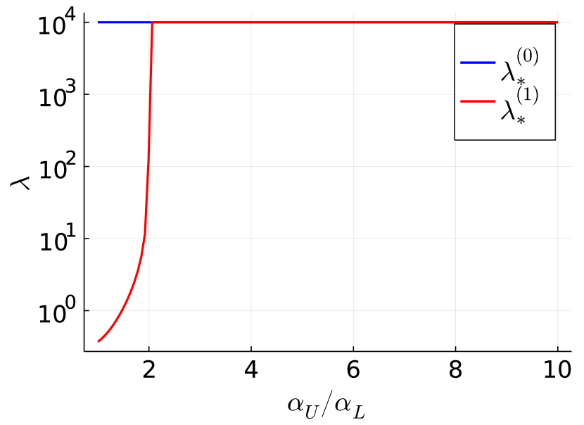
(a) $(\rho,\Delta)=(0.5,1.0)$

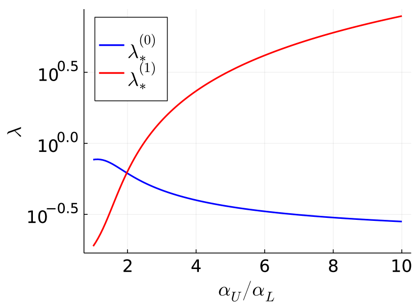
(b) $(\rho,\Delta)=(0.495,1.0)$

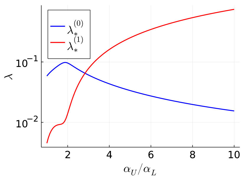
(c) $(\rho,\Delta)=(0.4,1.0)$

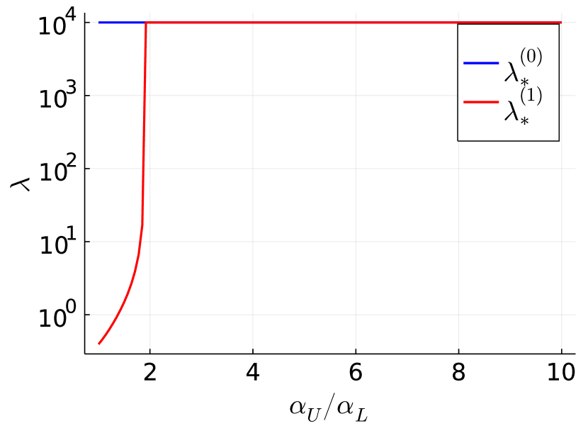
(d) $(\rho,\Delta)=(0.5,0.75^{2})$

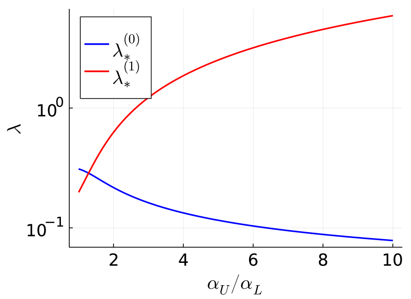
(e) $(\rho,\Delta)=(0.495,0.75^{2})$

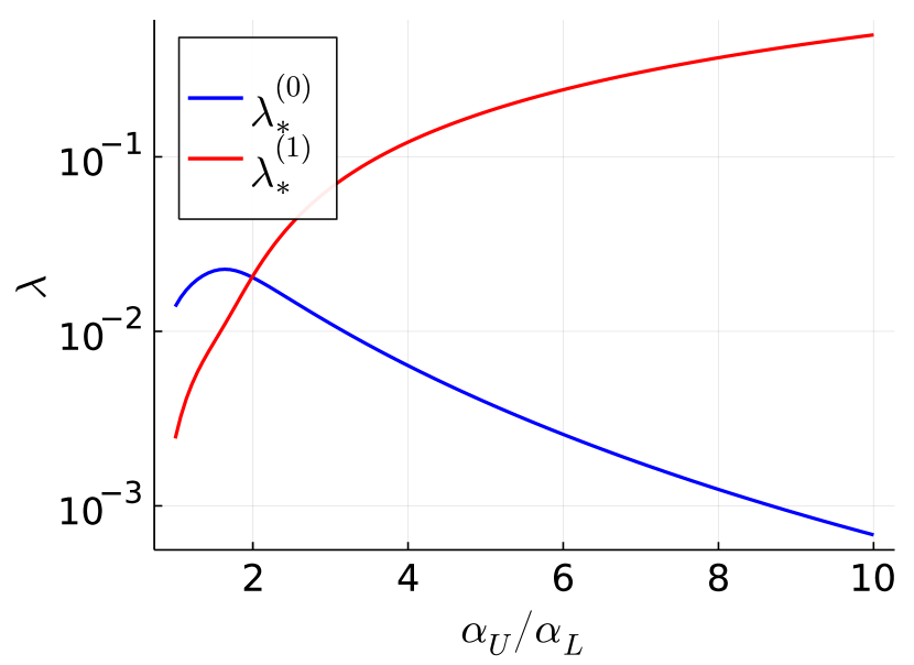
(f) $(\rho,\Delta)=(0.4,0.75^{2})$

Figure 1: The optimal regularization parameters $(\lambda^{(0)}_{\ast},\lambda^{(1)}_{\ast})$, which minimize the generalization error $\epsilon_{\rm g}^{(1)}$, are plotted against the relative number of unlabeled data points $\alpha_{U}/\alpha_{L}$. Each panel corresponds to the different values of $\rho$ and $\Delta$.

Figure 1 summarizes how the optimal regularization parameters $(\lambda^{(0)}_{\ast},\lambda^{(1)}_{\ast})$, which minimize the generalization error $\epsilon_{\rm g}^{(1)}$, depend on the size of the unlabeled dataset $\alpha_{U}$, the relative size of clusters $\rho$ and the size of each cluster $\Delta$. Each panel corresponds to different values of $\rho$ and $\Delta$. Except for the case of $\rho=0.5$, both $\lambda_{\ast}^{(0)}$ and $\lambda_{\ast}^{(1)}$ depend on the size of the unlabeled data $\alpha_{U}$. In this setup, the regularization parameter $\lambda^{\ast({\rm SL})}$, which is optimal for predicting a label for a new input, is not the best choice for giving the pseudo-labels. This result suggests that the ST with the regularized cross-entropy loss may require tuning all of the regularization parameters in $\mathbb{R}^{T+1}$ to achieve the best performance, unlike successively tuning the regularization parameters $\lambda^{(t)},t=0,1,\dots,T$ in $\mathbb{R}$ at each iteration step.

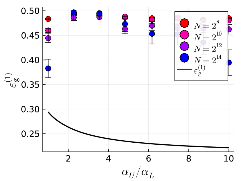
(a) $(\rho,\Delta)=(0.5,1.0)$

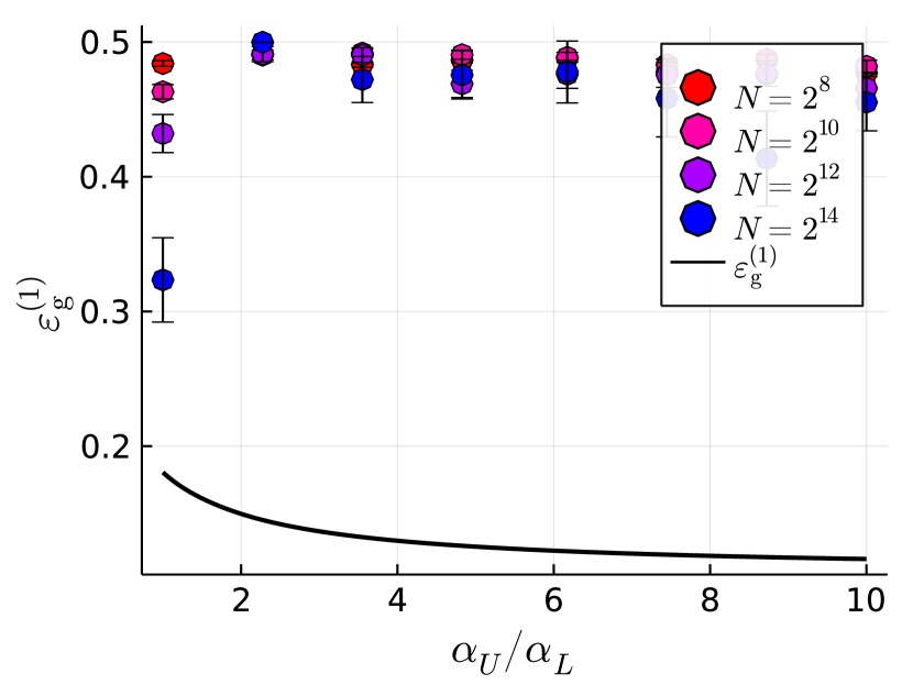
(b) $(\rho,\Delta)=(0.5,0.75^{2})$

Figure 2: Theoretical estimate for the optimal generalization error $\epsilon_{\rm g}^{(1)}$ for $\rho=0.5$ is compared with the experiments. The black solid line is the theoretical estimate in LSL, and the symbols represent the experimental results. Here the regularization parameter is limited as $(\lambda^{(0)},\lambda^{(1)})\in(0,10)^{2}$. For moderately large $\alpha_{U}$, $(\lambda^{(0)},\lambda^{(1)})=(10,10)$, however, for such large regularization parameters, the experimental results heavily suffer from large finite-size effects.

For $\rho=0.5$, the optimal regularization parameter for $\lambda^{(1)}$ shows a peculiar behavior: for $\alpha_{U}<\alpha_{U}^{\ast}$, the optimal regularization parameter $\lambda^{(1)}$ is finite, but above $\alpha_{U}^{\ast}$, it seems to diverge. The diverging tendency may be legitimate because the infinitely large regularization yields the Bayes-optimal classifier for supervised logistic regression with $\rho=0.5$ (Mignacco et al., 2020). However, the behavior for $\alpha_{U}<\alpha_{U}^{\ast}$ is rather unexpected. We also remark that the optimality of the infinitely large regularization parameter would hold only in LSL as already suggested in the supervised case (Mignacco et al., 2020). For finite $N$, huge regularization parameters do not give a good estimator. Indeed, we confirmed that even for $\lambda^{(0)}=\lambda^{(1)}=10$, the experimental results heavily suffer from finite-size effects (see figure 2). Thus, for $\rho=0.5$, we limit the range of the regularization parameters in the following so that the theoretical estimate has relevance to experiments with moderately large system sizes.

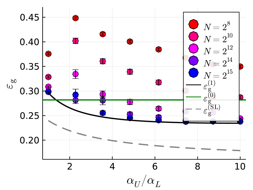
(a) $(\rho,\Delta)=(0.5,1.0)$

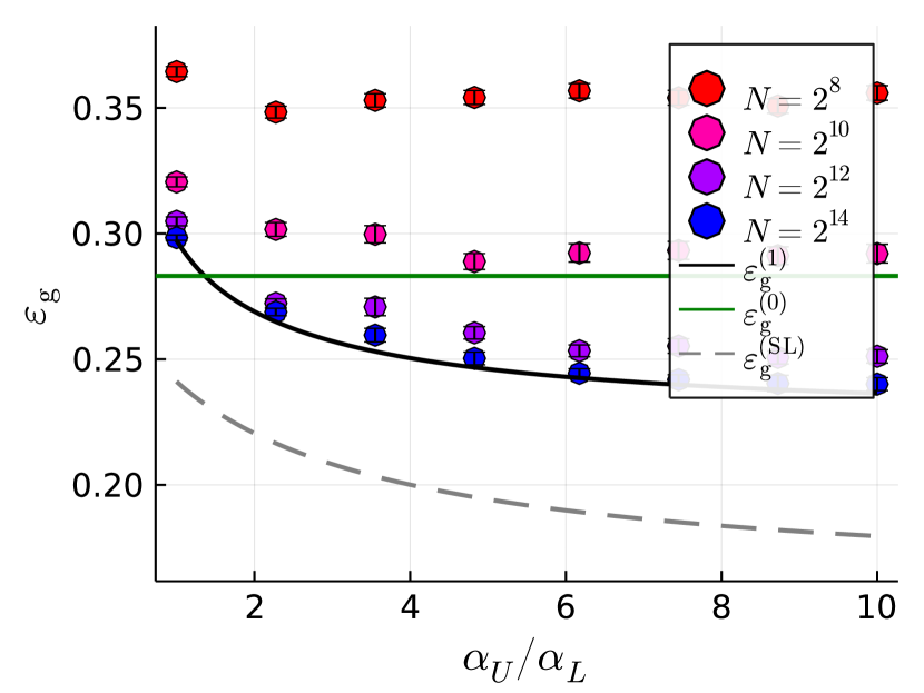
(b) $(\rho,\Delta)=(0.495,1.0)$

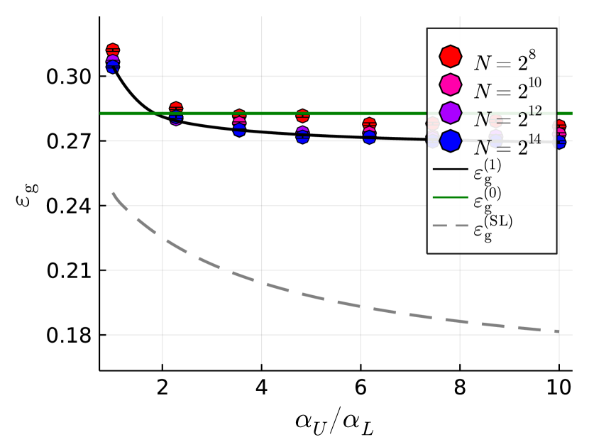
(c) $(\rho,\Delta)=(0.4,1.0)$

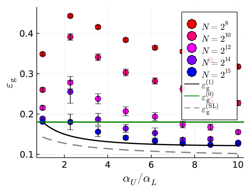
(d) $(\rho,\Delta)=(0.5,0.75^{2})$

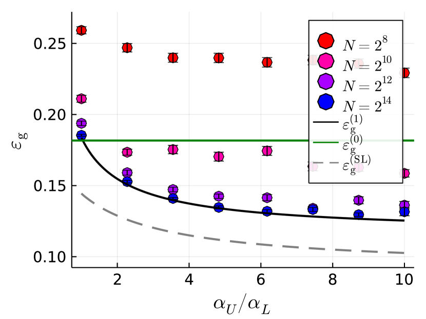
(e) $(\rho,\Delta)=(0.495,0.75^{2})$

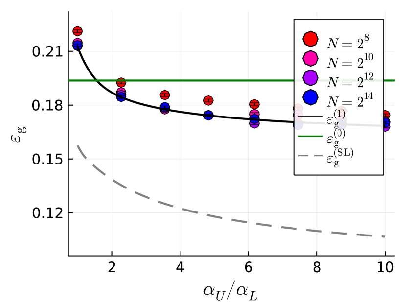
(f) $(\rho,\Delta)=(0.4,0.75^{2})$

Figure 3: Optimal generalization error for the single-shot ST $\epsilon_{\rm g}^{(1)}$ versus the relative number of unlabeled data $\alpha_{U}/\alpha_{L}$. The amount of labeled data is fixed as $\alpha_{L}=0.5$. The solid black line is the theoretical estimate in LSL. The symbols with error bars represent the results obtained from the numerical experiments with finite sizes. The optimal generalization error for $\epsilon_{\rm g}^{(0)}$ (solid green lines) and the generalization error for the supervised training with labeled data set of size $\alpha_{L}+\alpha_{U}$ (gray dashed lines) are also plotted for comparison. At $\alpha_{U}/\alpha_{L}=10$, total amount of the unlabeled data is $5N$ ($=10\alpha_{L}N$).

Figure 3 shows how the optimal generalization error depends on various control parameters. For sufficiently large unlabeled data size, the single-shot ST achieves a lower generalization error than the supervised learning with the labeled data of size $\alpha_{L}$. This result indicates the usefulness of the unlabeled data in ST. However, as $\rho$ deviates from $0.5$, the magnitude of the improvement obtained by the unlabeled data decreases. This result indicates that the single-shot ST is not so useful for biased data. In numerical experiments for $\rho=0.5$, we limit the values of the regularization parameters as $\lambda^{(0)}<0.5$ and $\lambda^{(1)}<5.0$ to avoid huge finite-size effects.

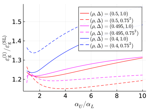
Figure 4: Relative generalization error against the generalization error obtained by supervised learning with data size $\alpha_{L}+\alpha_{U}$. The amount of the labeled data is fixed as $\alpha_{L}=0.5$.

Finally, Figure 4 summarizes how the generalization error performs compared to the generalization error $\epsilon_{\rm g}^{({\rm SL})}$ obtained by supervised learning with data size $\alpha_{L}+\alpha_{U}$. In any case, the ratio $\epsilon_{\rm g}^{(1)}/\epsilon_{\rm g}^{(\rm{SL})}$ slightly increases at large $\alpha_{U}$. This tendency is especially noticeable when two clusters have a large overlap, $\Delta$ is large, or the data are biased, $\rho\neq 0.5$. These results indicate that single-shot ST cannot efficiently use the unlabeled data even when the regularization parameters are optimized.

The next subsection investigates how the iterative learning procedure improves the single-shot ST.

4.2 Iterative ST, the case of $T>1$

In the previous section, we have seen that the unlabeled data can improve the generalization performance, even in the single-shot ST. In this subsection, we proceed to investigate whether the iterative ST with $T>1$ could further enhance the generalization performance.

Although the results of the single-shot case suggest that we may need to fine-tune all of the regularization parameters in $\mathbb{R}^{T+1}$, it is computationally demanding. Thus, we optimize the regularization parameters while imposing the constraint that $\lambda^{(1)}=\lambda^{(2)}=\dots=\lambda^{(T)}$.

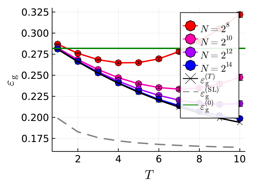
(a) $(\rho,\Delta)=(0.5,1.0)$

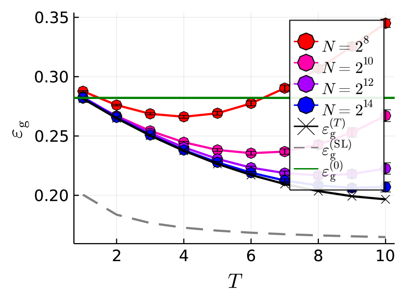
(b) $(\rho,\Delta)=(0.495,1.0)$

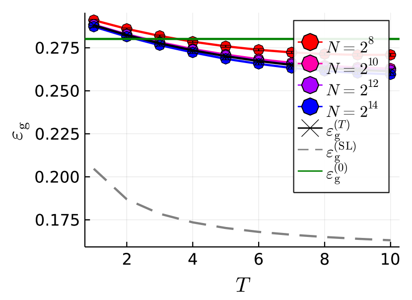
(c) $(\rho,\Delta)=(0.4,1.0)$

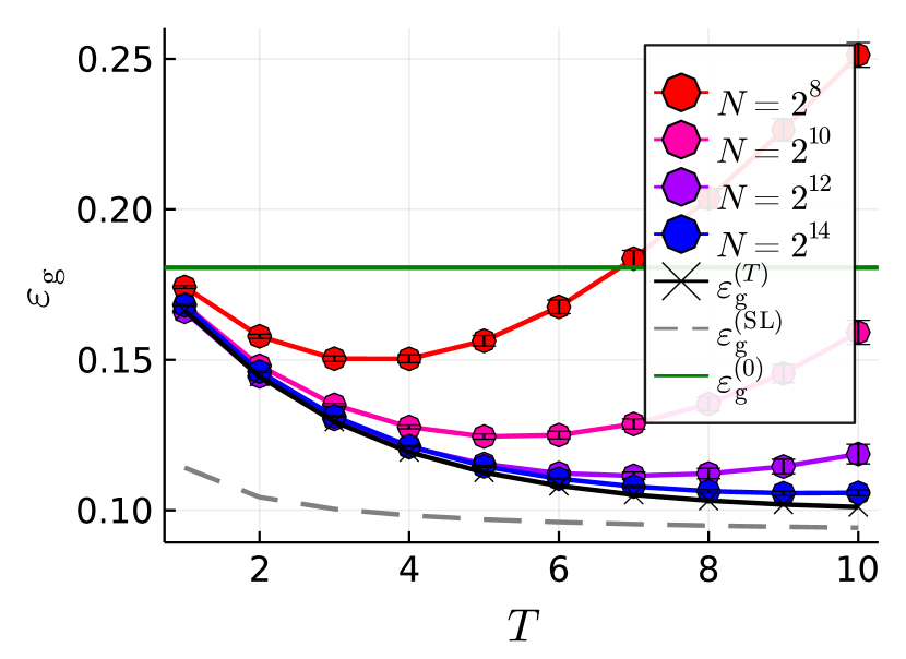
(d) $(\rho,\Delta)=(0.5,0.75^{2})$

(e) $(\rho,\Delta)=(0.495,0.75^{2})$

(f) $(\rho,\Delta)=(0.4,0.75^{2})$

Figure 5: Optimal generalization error for the iterative ST $\epsilon_{\rm g}^{(T)}$ versus the number of iterations $T\in\{1,2,\dots,10\}$. The amount of the labeled data is fixed as $\alpha_{L}=0.5$, and at each iteration, unlabeled data with size $\alpha_{U}=2.0$ is used. The solid black line is the theoretical estimate in LSL. The symbols with error bars represent the results obtained from the numerical experiments with finite sizes. The optimal generalization error for $\epsilon_{\rm g}^{(0)}$ (solid green lines) and the generalization error for the supervised training with labeled data set of size $\alpha_{L}+t\alpha_{U}$ (gray dashed lines) are also plotted for comparison. At $T=10$, the total amount of unlabeled data is $20N$ ($=10\alpha_{U}N$).

Figure 5 shows how the optimal generalization error depends on various control parameters in iterative ST. In all cases, we see that the generalization error gradually decreases as the number of iterations grows. This decreasing tendency continues to a relatively large iteration number, and the generalization errors at $T=10$ are generally smaller than the saturated generalization errors in single-shot ST with large $\alpha_{U}$. This suggests that the iterative ST can successfully manage to use the large unlabeled data with a rather simple regularization schedule. However, the improvement becomes smaller when the data has a large bias ($\rho\ll 0.5$). In numerical experiments for $\rho=0.5$, we limit the values of the regularization parameters as $\lambda^{(0)}=\lambda^{(1)}=\dots=\lambda^{(T)}<0.1$ to avoid huge finite-size effects.

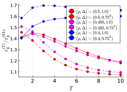
Figure 6: Relative generalization error against the generalization error obtained by supervised learning with data size $\alpha_{L}+T\alpha_{U}$. The amount of the labeled data is fixed as $\alpha_{L}=0.5$. At $T=10$, the total amount of unlabeled data is $20N$ $(=10\alpha_{U}N)$.

Finally, the relative performance against the supervised learning with data size $\alpha_{L}+T\alpha_{U}$ is plotted in Figure 6. For $\rho=0.5$ and $0.495$, the ratio against the supervised case decreases with the number of iterations. This tendency differs from the single-shot case in which the relative performance degrades with large unlabeled data. Notice that the total amount of the unlabeled data at $T=10$ is $10\alpha_{U}N=20N$ that is four times greater than the largest unlabeled data used in the single-shot ST. However, the relative performance sticks at large values for heavily biased cases with $\rho\ll 0.5$, which is the same behavior as the single-shot case. These results again support the superiority of iterative ST against the single-shot ST, for nearly unbiased data with $\rho\simeq 0.5$.

5 Summary and conclusion

In this work, we developed a theoretical framework for analyzing the iterative ST, when different data are used at each training step, using the replica method of statistical physics. We applied the developed theoretical framework to the iterative ST that uses the ridge-regularized cross-entropy loss at each training step. In particular, we considered the data generation model in which each data point is generated from a binary Gaussian mixture with general variance of each cluster $\Delta$ and relative size of the clusters $\rho$. Consequently, we derived a set of deterministic, self-consistent equations of a small finite number of variables that sharply characterize the generalization error at arbitrary iteration steps.

Based on the derived formula, we were able to quantitatively investigate the role of the regularization parameters used at each step and the iterative learning procedure. In particular, we found that even the single-shot ST could find a model with a better generalization performance than the model obtained by the logistic regression on the labeled data only. Furthermore, when $\rho$ is close to $0.5$, the iterative learning procedure with a relatively simple regularization schedule further decreases the generalization error. The achieved generalization error approached the one obtained by the logistic regression when the ground truth labels are known for all data points. These results suggest that we could handle large, unlabeled data with a simple, iterative ST when the data have a small bias. However, the magnitude of the improvement obtained by iterative ST soon deteriorates as the $\rho$ deviates from $0.5$, resulting in a much larger generalization error than the supervised logistic regression. For such biased data, we might need a more sophisticated methodology.

Unsatisfactory aspects of the present work include the non-rigorous nature of the replica method and the very simple architecture of the learning model. The former non-rigorousness might be resolved using the techniques developed in analyzing other convex learning problems (Mignacco et al., 2020; Gerbelot et al., 2020). For simplification of the model architecture, we might be able to extend the present analysis based on the previous analytical techniques to handle the replicated system for more complex model architectures, such as the random feature model (Gerace et al., 2020), kernel method (Canatar et al., 2021; Dietrich et al., 1999), and multi-layer neural networks (Schwarze and Hertz, 1992; Yoshino, 2020).

Quantitatively comparing with other semi-supervised learning methods such as the entropy regularization (Grandvalet and Bengio, 2006) is also a natural future research direction. Another natural but challenging direction is to extend our analysis to the case in which the same unlabeled data are used in each iteration. However, sharply characterizing the performance might be much more involved because the correlations between the models obtained at different iterations would need to be handled carefully.

Acknowledgments

This study was supported by JSPS KAKENHI Grant Number 21K21310.

Appendix A Replica method calculation

In this appendix, we outline the replica calculation leading to the claims 1-3. We consider an even more general setting whereby the cross-entropy loss and the sigmoid pseudo-label is replaced by an arbitrary convex function and an arbitrary differentiable monotonously increasing function, respectively. Namely, instead of minimizing the ridge-regularize cross-entropy loss, we consider minimizing the general ridge-regularized convex empirical risk minimization problem with the arbitrary differentiable pseudo label, or, the cost functions used for the supervised learning at $t=0$ and the self-training at $t>0$ take the following form:

$$\tilde{\mathcal{L}}^{(0)}(\mathbf{\boldsymbol{\theta}}^{(0)};D_{L}) =\sum_{\mu=1}^{M_{L}}\tilde{l}\left(y_{\mu},\sigma\left(\frac{1}{\sqrt{N}}(\mathbf{\boldsymbol{x}}_{\mu}^{(0)})^{\top}\mathbf{\boldsymbol{w}}^{(0)}+b^{(0)}\right)\right)+\frac{\lambda^{(0)}}{2}\|\mathbf{\boldsymbol{w}}^{(0)}\|_{2}^{2},$$ (67)

$$\tilde{\mathcal{L}}^{(t)}(\mathbf{\boldsymbol{\theta}}^{(t)};D_{U}^{(t)},\mathbf{\boldsymbol{\theta}}^{(t-1)}) =\sum_{\nu=1}^{M_{U}}\tilde{l}\left(\tilde{\sigma}\left(\frac{1}{\sqrt{N}}(\mathbf{\boldsymbol{x}}_{\nu}^{(t)})^{\top}\mathbf{\boldsymbol{w}}^{(t-1)}+b^{(t-1)}\right),\right.$$

$$\hskip 30.0pt\left.\sigma\left(\frac{1}{\sqrt{N}}(\mathbf{\boldsymbol{x}}_{\nu}^{(t)})^{\top}\mathbf{\boldsymbol{w}}^{(t)}+b^{(t)}\right)\right)+\frac{\lambda^{(t)}}{2}\|\mathbf{\boldsymbol{w}}^{(t)}\|_{2}^{2},\quad t=1,2,\dots,T,$$ (68)

with $\tilde{l}$ being a convex loss function and $\tilde{\sigma}$ being the differentiable monotonically increasing function. Important examples for the loss function include the squared error loss and the cross-entropy loss. For the pseudo-label, the examples include the sigmoid function with the temperature $\gamma$: $\tilde{\sigma}(x)=1/(1+e^{-\gamma x})$. The claims 1-3 are generalized to the present setting by replacing the cross-entropy loss $l$ and the sigmoid function $\sigma$ with $\tilde{l}$ and $\tilde{\sigma}$, respectively.

A.1 Replica method for iterative ST

We begin with recalling the basic strategy for evaluating free energy using the non-rigorous replica method of statistical physics. The average of the free energy can be evaluated as:

$$f^{(T)} =\lim_{N,\beta\to\infty}\mathbb{E}_{D,\{\mathbf{\boldsymbol{\theta}}^{(t)}\}_{t=0}^{T-1}}\left[\frac{1}{\beta^{(T)}N}\log Z^{(T)}(D_{U}^{(T)},\mathbf{\boldsymbol{\theta}}^{(T-1)};\beta^{(T)})\right],$$ (69)

$$=\lim_{N,\beta\to\infty}\mathbb{E}_{D}\left[\int\frac{1}{\beta^{(T)}N}\log Z^{(T)}(D_{U}^{(T)},\mathbf{\boldsymbol{\theta}}^{(T-1)})\frac{1}{Z^{(0)}(D_{L})}e^{-\beta^{(0)}\tilde{\mathcal{L}}^{(0)}(\mathbf{\boldsymbol{\theta}}^{(0)};D_{L})}\right.$$

$$\left.\times\prod_{t=1}^{T-1}\frac{1}{Z^{(t)}(D_{U}^{(t)},\mathbf{\boldsymbol{\theta}}^{(t-1)})}e^{-\beta^{(t)}\tilde{\mathcal{L}}^{(t)}(\mathbf{\boldsymbol{\theta}}^{(t)};D_{U}^{(t)},\mathbf{\boldsymbol{\theta}}^{(t-1)})}d\mathbf{\boldsymbol{\theta}}^{(0)}\dots d\mathbf{\boldsymbol{\theta}}^{(T-1)}\right]$$ (70)

The key observation here is that we have to evaluate the average of the logarithm and the inverse of the normalization constants, which make the evaluation of free energy technically difficult in general. To resolve these difficulties in computing the free energy, we resort to two types of the replica methods (Mézard et al., 1987; Mézard and Montanari, 2009; Parisi et al., 2020).

First, we use the replica method that rewrites the above free energy using the identities $\lim_{n_{T}\to 0}n_{T}^{-1}\log\mathbb{E}[(Z^{(T)})^{n_{T}}]=\mathbb{E}[\log Z^{(T)}]$ as

$$f^{(T)} =\lim_{n^{(T)}\to 0}\frac{1}{n_{T}}\tilde{\phi}_{n_{T}}^{(T)},$$ (71)

$$\tilde{\phi}_{n_{T}}^{(T)} =\lim_{N,\beta\to\infty}\frac{1}{N\beta^{(T)}}\log\mathbb{E}_{D,\{\mathbf{\boldsymbol{\theta}}^{(t)}\}_{t=0}^{T-1}}\left[(Z^{(T)})^{n_{T}}\right].$$ (72)

Although the evaluation of $\tilde{\phi}_{n_{T}}^{(T)}$ for $n_{T}\in\mathbb{R}$ is difficult, still, this expression has an advantage. For $n_{T}=1,2,\dots,$ using the identity

$$(Z^{(T)})^{n_{T}} =\left(\int e^{-\beta^{(T)}\tilde{\mathcal{L}}^{(T)}(\mathbf{\boldsymbol{\theta}}^{(T)};D_{U}^{(T)},\mathbf{\boldsymbol{\theta}}^{(T-1)})}d\mathbf{\boldsymbol{\theta}}^{(T)}\right)^{n_{T}}$$

$$=\int\prod_{c_{T}=1}^{n_{T}}e^{-\beta^{(T)}\tilde{\mathcal{L}}^{(T)}(\mathbf{\boldsymbol{\theta}}_{c_{T}}^{(T)};D_{U}^{(T)},\mathbf{\boldsymbol{\theta}}^{(T-1)})}d\mathbf{\boldsymbol{\theta}}_{1}^{(T)}\dots d\mathbf{\boldsymbol{\theta}}_{n_{T}}^{(T)},$$ (73)

$\tilde{\phi}^{(T)}_{n_{T}}$ can be expressed as follows:

$$\tilde{\phi}_{n_{T}}^{(T)}=\lim_{N,\beta\to\infty}\frac{1}{N\beta^{(T)}}\log\int\mathbb{E}_{D,\{\mathbf{\boldsymbol{\theta}}^{(t)}\}_{t=0}^{T-1}}\left[\prod_{c_{T}=1}^{n_{T}}e^{-\beta^{(T)}\mathcal{L}^{(T)}(\mathbf{\boldsymbol{\theta}}_{c_{T}}^{(T)};D_{U}^{(T)},\mathbf{\boldsymbol{\theta}}^{(T-1)})}\right]d\mathbf{\boldsymbol{\theta}}_{1}^{(T)}\dots d\mathbf{\boldsymbol{\theta}}_{n_{T}}^{(T)}.$$ (74)

This expression is more favorable because we can eliminate the average of the logarithm. However, the inverse of the normalization constants $(Z^{(0)}(D_{L}))^{-1}\prod_{t=1}^{T-1}(Z^{(t)}(D_{U}^{(t)},\mathbf{\boldsymbol{\theta}}^{(t-1)}))^{-1}$ in the integrand of (74) must be averaged, which is difficult.

To resolve this difficulty, we use another form of the replica method. This method rewrites $\tilde{\phi}_{n_{T}}^{(T)}$ using the trivial identity $(Z^{(t)})^{-1}=\lim_{n_{t}\to 0}(Z^{(t)})^{n_{t}-1}$ as

$$\tilde{\phi}_{n_{T}}^{(T)} =\lim_{n_{0},\dots,n_{T-1}\to 0}\phi_{n_{0},n_{1},\dots,n_{T}}^{(T)}$$ (75)

$$\phi_{n_{0},n_{1},\dots,n_{T}}^{(T)} =\lim_{N,\beta\to\infty}\frac{1}{N\beta^{(T)}}\log\int\mathbb{E}_{D}\left[\prod_{c_{T}=1}^{n_{T}}e^{-\beta^{(T)}\tilde{\mathcal{L}}^{(0)}(\mathbf{\boldsymbol{\theta}}_{c_{T}};D_{U}^{(T)},\mathbf{\boldsymbol{\theta}}^{(T-1)})}\right.$$

$$\left.\times(Z^{(0)}(D_{L}))^{n_{0}-1}e^{-\beta^{(0)}\tilde{\mathcal{L}}(\mathbf{\boldsymbol{\theta}}^{(0)};D_{L})}\right.$$

$$\left.\times\prod_{t=1}^{T-1}(Z^{(t)}(D_{U}^{(t)},\mathbf{\boldsymbol{\theta}}^{(t-1)}))^{n_{t}-1}e^{-\beta^{(t)}\tilde{\mathcal{L}}^{(t)}(\mathbf{\boldsymbol{\theta}}^{(t)};D_{U}^{(t)},\mathbf{\boldsymbol{\theta}}^{(t-1)})}d\mathbf{\boldsymbol{\theta}}^{(0)}\dots d\mathbf{\boldsymbol{\theta}}^{(T-1)}\right]d\mathbf{\boldsymbol{\theta}}_{1}^{(T)}\dots\mathbf{\boldsymbol{\theta}}_{n_{T}}^{(T)}.$$ (76)

Again, although rigorously evaluating $\phi_{n_{0},n_{1},\dots,n_{T}}^{(T)}$ for $n_{0},n_{1},\dots,n_{T-1}\in\mathbb{R}$ is difficult, for integers $n_{0},n_{1},\dots,n_{T-1}=1,2,\dots$ it has an appealing expression:

$$\phi_{n_{0},n_{1},\dots,n_{T}}^{(T)}=\lim_{N,\beta\to\infty}\frac{1}{N\beta^{(T)}}\log\int\mathbb{E}_{D}\left[\prod_{c_{0}=1}^{n_{0}}e^{-\beta^{(0)}\tilde{\mathcal{L}}^{(0)}(\mathbf{\boldsymbol{\theta}}_{c_{0}}^{(0)};D_{L})}\right.$$

$$\left.\times\prod_{t=1}^{T}\prod_{c_{t}=1}^{n_{t}}e^{-\beta^{(t)}\tilde{\mathcal{L}}^{(t)}(\mathbf{\boldsymbol{\theta}}_{c_{t}}^{(t)};D_{U}^{(t-1)},\mathbf{\boldsymbol{\theta}}_{1}^{(t-1)})}\right]d^{n_{0}}\mathbf{\boldsymbol{\theta}}^{(0)}\dots d^{n_{T}}\mathbf{\boldsymbol{\theta}}^{(T)}.$$ (77)

The replicated system (77) is much easier to handle than the original problem of averaging the logarithm because all of the factors to be evaluated are now explicit. The replica method evaluates a formal expression of $\phi^{(T)}_{n_{0},n_{1},\dots,n_{T}}$ for $n_{0},n_{1},\dots,n_{T}=1,2,\dots$ and then extrapolates it as $n\to 0$.

A.2 Derivation of the RS saddle point condition

We next consider how to evaluate the replicated system (77) using the RS assumption and saddle point method.

Inserting the explicit form of the loss functions (67)-(68) and the feature vectors (1)-(2) into (77), we obtain the following:

$$\phi^{(T)}_{n_{0},n_{1},\dots,n_{T}} =\lim_{N,\beta\to\infty}\frac{1}{N\beta^{(T)}}\log\int\prod_{\mu=1}^{M_{L}}\mathbb{E}_{y_{\mu}^{(0)},\mathbf{\boldsymbol{x}}_{\mu}^{(0)}}\left[\prod_{c_{0}=1}^{n_{0}}e^{-\beta^{(0)}\tilde{l}\left(y_{\mu}^{(0)},\sigma\left(h_{c_{0},\mu}^{(0)}\right)\right)}\right]$$

$$\times\prod_{t=1}^{T}\prod_{\nu=1}^{M_{U}}\mathbb{E}_{y_{\nu}^{(t)},\mathbf{\boldsymbol{x}}_{\nu}^{(t)}}\left[\prod_{c_{t}=1}^{n_{t}}e^{-\beta^{(t)}\tilde{l}\left(\tilde{\sigma}\left(\tilde{h}_{c_{t},\nu}^{(t)}\right),\sigma\left(h_{c_{t},\nu}^{(t)}\right)\right)}\right]$$

$$\times\prod_{t=0}^{T}\prod_{i=1}^{N}\prod_{c_{t}=1}^{n_{t}}e^{-\frac{\beta^{(t)}\lambda^{(t)}}{2}(w_{c_{t},i}^{(t)})^{2}}d^{n_{0}}\mathbf{\boldsymbol{\theta}}^{(0)}\dots d^{n_{T}}\mathbf{\boldsymbol{\theta}}^{(T)},$$ (78)

with the notations

$$h_{c_{0},\mu}^{(0)} =(2y_{\mu}^{(0)}-1)\frac{1}{N}(\mathbf{\boldsymbol{w}}_{c_{0}}^{(0)})^{\top}\mathbf{\boldsymbol{v}}+b_{c_{0}}^{(0)}+\frac{1}{\sqrt{N}}(\mathbf{\boldsymbol{w}}_{c_{0}}^{(0)})^{\top}\mathbf{\boldsymbol{z}}_{\mu}^{(0)},$$ (79)

$$\tilde{h}_{c_{t},\nu}^{(t)} =(2y_{\nu}^{(t)}-1)\frac{1}{N}(\mathbf{\boldsymbol{w}}_{1}^{(t-1)})^{\top}\mathbf{\boldsymbol{v}}+b_{1}^{(t-1)}+\frac{1}{\sqrt{N}}(\mathbf{\boldsymbol{w}}_{1}^{(t-1)})^{\top}\mathbf{\boldsymbol{z}}_{\nu}^{(t)},$$ (80)

$$h_{c_{,}\nu}^{(t)} =(2y_{\nu}^{(t)}-1)\frac{1}{N}(\mathbf{\boldsymbol{w}}_{1}^{(t)})^{\top}\mathbf{\boldsymbol{v}}+b_{c_{t}}^{(t)}+\frac{1}{\sqrt{N}}(\mathbf{\boldsymbol{w}}_{1}^{(t)})^{\top}\mathbf{\boldsymbol{z}}_{\nu}^{(t)}.$$ (81)

At this point, we can take the average with respect to the noise $\mathbf{\boldsymbol{z}}_{\mu}^{(0)}$, $\mathbf{\boldsymbol{z}}_{\nu}^{(t)}$. We use the fact that, from the iid Gaussian assumptions on these noise vectors, the vectors

$$\mathbf{\boldsymbol{u}}_{\mu}^{(0)} =\left(\frac{1}{\sqrt{N}}(\mathbf{\boldsymbol{w}}_{1}^{(0)})^{\top}\mathbf{\boldsymbol{z}}_{\mu}^{(0)},\frac{1}{\sqrt{N}}(\mathbf{\boldsymbol{w}}_{2}^{(0)})^{\top}\mathbf{\boldsymbol{z}}_{\mu}^{(0)},\dots,\frac{1}{\sqrt{N}}(\mathbf{\boldsymbol{w}}_{n_{0}}^{(0)})^{\top}\mathbf{\boldsymbol{z}}_{\mu}^{(0)}\right)^{\top}\in\mathbb{R}^{n_{0}},$$ (82)

$$\mathbf{\boldsymbol{u}}_{\nu}^{(t)} =\left(\frac{1}{\sqrt{N}}(\mathbf{\boldsymbol{w}}_{1}^{(t-1)})^{\top}\mathbf{\boldsymbol{z}}_{\nu}^{(t)},\frac{1}{\sqrt{N}}(\mathbf{\boldsymbol{w}}_{1}^{(t)})^{\top}\mathbf{\boldsymbol{z}}_{\nu}^{(t)},\frac{1}{\sqrt{N}}(\mathbf{\boldsymbol{w}}_{2}^{(t)})^{\top}\mathbf{\boldsymbol{z}}_{\nu}^{(t)},\dots,\frac{1}{\sqrt{N}}(\mathbf{\boldsymbol{w}}_{n_{t}}^{(t)})^{\top}\mathbf{\boldsymbol{z}}_{\nu}^{(t)}\right)^{\top}\in\mathbb{R}^{n_{t}+1},$$

$$t =1,2,\dots,T,$$ (83)

can be independently handled as zero-mean multivariate Gaussian variables:

$$\mathbf{\boldsymbol{u}}_{\mu}^{(0)} \sim_{\rm iid}\mathcal{N}(0,\Sigma^{(0)}),\quad\Sigma^{(0)}=\Delta\times\left[\begin{array}[]{ccc}Q_{11}^{(0)}&\cdots&Q_{1n_{0}}^{(0)}\\ \vdots&\ddots&\vdots\\ Q_{n_{0}1}^{(0)}&\cdots&Q_{n_{0}n_{0}}^{(0)}\end{array}\right],$$ (87)

$$Q_{c_{0}d_{0}}^{(0)} \equiv\frac{1}{N}(\mathbf{\boldsymbol{w}}_{c_{0}}^{(0)})^{\top}\mathbf{\boldsymbol{w}}_{d_{0}}^{(0)},\quad c_{0},d_{0}=1,2,\dots,n_{0},$$ (88)

and

$$\mathbf{\boldsymbol{u}}_{\nu}^{(t)} \sim_{\rm iid}\mathcal{N}(0,\Sigma^{(t)}),\quad\Sigma^{(t)}=\Delta\times\left[\begin{array}[]{c|ccc}Q_{11}^{(t-1)}&R_{1}^{(t)}&\cdots&R_{n_{t}}^{(t)}\\ \hline\cr R_{1}^{(t)}&Q_{11}^{(t)}&\cdots&Q_{1n_{t}}^{(t)}\\ \vdots&\vdots&\ddots&\vdots\\ R_{n_{t}}^{(t)}&Q_{n_{t}1}^{(t)}&\cdots&Q_{n_{t}n_{t}}^{(t)}\end{array}\right]$$ (93)

$$Q_{c_{t}d_{t}}^{(t)} =\frac{1}{N}(\mathbf{\boldsymbol{w}}^{(t)}_{c_{t}})^{\top}\mathbf{\boldsymbol{w}}_{d_{t}}^{(t)},\quad R_{c_{t}}^{(t)}=\frac{1}{N}(\mathbf{\boldsymbol{w}}^{(t-1)}_{1})^{\top}\mathbf{\boldsymbol{w}}_{c_{t}}^{(t)},\quad c_{t},d_{t}=1,2,\dots,n_{t},$$ (94)

for a fixed set of $\mathbf{\boldsymbol{w}}_{c_{0},\mu}^{(0)},\mathbf{\boldsymbol{w}}_{c_{t},\nu}^{(t)}$, $c_{0}=1,2,\dots,n_{0},c_{t}=1,2,\dots,n_{t}$, $\mu=1,2,\dots,M_{L}$, and $\nu=1,2,\dots,M_{U}$. Thus, the replicated system (78) depends on $\mathbf{\boldsymbol{w}}_{c_{t}}^{(t)},c_{t}=1,2,\dots,n_{t},t=0,1,\dots,T$ only through their inner products, such as

$$\frac{1}{N}(\mathbf{\boldsymbol{w}}_{c_{t}}^{(t)})^{\top}\mathbf{\boldsymbol{w}}_{d_{t}}^{(t)},\quad c_{t},d_{t}=1,2,\dots,n_{t},\;t=0,1,\dots T,$$ (95)

$$\frac{1}{N}(\mathbf{\boldsymbol{w}}_{c_{t}}^{(t)})^{\top}\mathbf{\boldsymbol{v}},\quad c_{t}=1,\dots,n_{t},\;t=0,1,\dots,T,$$ (96)

$$\frac{1}{N}(\mathbf{\boldsymbol{w}}_{1}^{(t-1)})^{\top}\mathbf{\boldsymbol{w}}_{c_{t}}^{(t)},\quad c_{t}=1,2,\dots,n_{t},\;t=1,\dots,T,$$ (97)

which capture the geometric relations between the estimators and the centroid of data distribution $\mathbf{\boldsymbol{v}}$. We introduce the auxiliary variables through the trivial identities

$$1 =\prod_{t=0}^{T}\prod_{1\leq c_{t}\leq d_{t}\leq n_{t}}N\int\delta\left(NQ_{c_{t}d_{t}}^{(t)}-(\mathbf{\boldsymbol{w}}_{c_{t}}^{(t)})^{\top}\mathbf{\boldsymbol{w}}_{d_{t}}^{(t)}\right)dQ_{c_{t}d_{t}}^{(t)},$$ (98)

$$1 =\prod_{t=0}^{T}\prod_{c_{t}=1}^{n_{t}}N\int\delta\left(Nm_{c_{t}}^{(t)}-(\mathbf{\boldsymbol{w}}_{c_{t}}^{(t)})^{\top}\mathbf{\boldsymbol{v}}\right)dm_{c_{t}}^{(t)},$$ (99)

$$1 =\prod_{t=1}^{T}\prod_{c_{t}=1}^{n_{t}}N\int\delta\left(NR_{c_{t}}^{(t)}-(\mathbf{\boldsymbol{w}}_{1}^{(t-1)})^{\top}\mathbf{\boldsymbol{w}}_{c_{t}}^{(t)}\right)dR_{c_{t}}^{(t)},$$ (100)

and the Fourier representations of the delta functions

$$\delta\left(NQ_{c_{t}d_{t}}^{(t)}-(\mathbf{\boldsymbol{w}}_{c_{t}}^{(t)})^{\top}\mathbf{\boldsymbol{w}}_{d_{t}}^{(t)}\right) =\int e^{\frac{\tilde{Q}_{c_{t}d_{t}}^{(t)}}{2}(NQ_{c_{t}d_{t}}^{(t)}-(\mathbf{\boldsymbol{w}}_{c_{t}}^{(t)})^{\top}\mathbf{\boldsymbol{w}}_{d_{t}}^{(t)})}\frac{d\tilde{Q}_{c_{t}d_{t}}^{(t)}}{4\pi},$$ (101)

$$\delta\left(Nm_{c_{t}}^{(t)}-(\mathbf{\boldsymbol{w}}_{c_{t}}^{(t)})^{\top}\mathbf{\boldsymbol{v}}\right) =\int e^{-\tilde{m}_{c_{t}}^{(t)}(Nm_{c_{t}}^{(t)}-(\mathbf{\boldsymbol{w}}_{c_{t}}^{(t)})^{\top}\mathbf{\boldsymbol{v}})}\frac{d\tilde{m}_{c_{t}}^{(t)}}{2\pi},$$ (102)

$$\delta\left(NR_{c_{t}}^{(t)}-(\mathbf{\boldsymbol{w}}_{1}^{(t-1)})^{\top}\mathbf{\boldsymbol{w}}_{c_{t}}^{(t)})\right) =\int e^{-\tilde{R}_{c_{t}}^{(t)}(NR_{c_{t}}^{(t)}-(\mathbf{\boldsymbol{w}}_{1}^{(t-1)})^{\top}\mathbf{\boldsymbol{w}}_{c_{t}}^{(t)})}\frac{d\tilde{R}_{c_{t}}^{(t)}}{2\pi},$$ (103)

into the integrand in (78). Let $\mathbf{\boldsymbol{\Theta}}$ and $\tilde{\mathbf{\boldsymbol{\Theta}}}$ be the collection of the variables

$$Q^{(t)} =[Q_{c_{t}d_{t}}^{(t)}]_{\begin{subarray}{c}1\leq c_{t}\leq n_{t}\\ 1\leq d_{t}\leq n_{t}\end{subarray}},\;\mathbf{\boldsymbol{m}}^{(t)}=[m_{c_{t}}^{(t)}]_{1\leq c_{t}\leq n_{t}},\;\mathbf{\boldsymbol{R}}^{(t)}=[R_{c_{t}}^{(t)}]_{1\leq c_{t}\leq n_{t}},\;\mathbf{\boldsymbol{b}}^{(t)}=[b_{c_{t}}^{(t)}]_{1\leq c_{t}\leq n_{t}},$$ (104)

and

$$\tilde{Q}^{(t)} =[\tilde{Q}_{c_{t}d_{t}}^{(t)}]_{\begin{subarray}{c}1\leq c_{t}\leq n_{t}\\ 1\leq d_{t}\leq n_{t}\end{subarray}},\;\tilde{\mathbf{\boldsymbol{m}}}^{(t)}=[\tilde{m}_{c_{t}}^{(t)}]_{1\leq c_{t}\leq n_{t}},\;\tilde{\mathbf{\boldsymbol{R}}}^{(t)}=[\tilde{R}_{c_{t}}^{(t)}]_{1\leq c_{t}\leq n_{t}},$$ (105)

respectively. Then, $\phi_{n_{0},n_{1},\dots,n_{T}}^{(T)}$ can be written as

$$\phi_{n_{0},n_{1},\dots,n_{T}}^{(T)} =\lim_{N,\beta\to\infty}\frac{1}{N\beta^{(T)}}\log\int e^{N\mathcal{S}^{(T)}(\mathbf{\boldsymbol{\Theta}},\tilde{\mathbf{\boldsymbol{\Theta}}})}d\mathbf{\boldsymbol{\Theta}}d\tilde{\mathbf{\boldsymbol{\Theta}}},$$ (106)

$$\mathcal{S}^{(T)}(\mathbf{\boldsymbol{\Theta}},\tilde{\mathbf{\boldsymbol{\Theta}}}) =\sum_{t=0}^{T}\left(\frac{1}{2}{\rm Tr}Q^{(t)}\tilde{Q}^{(t)}-(\mathbf{\boldsymbol{m}}^{(t)})^{\top}\tilde{\mathbf{\boldsymbol{m}}}^{(t)}\right)-\sum_{t=1}^{T}(\mathbf{\boldsymbol{R}}^{(t)})^{\top}\tilde{\mathbf{\boldsymbol{R}}}^{(t)}$$

$$+\alpha_{L}\log\int e^{-\tilde{\psi}_{w}(\mathbf{\boldsymbol{w}}^{(0)},\dots,\mathbf{\boldsymbol{w}}^{(T)})}d\mathbf{\boldsymbol{w}}^{(0)}.\dots d\mathbf{\boldsymbol{w}}^{(T)}$$

$$+\alpha_{U}\log\mathbb{E}_{y\sim p_{y}}\left[\int e^{-\tilde{\psi}_{u}^{(0)}(\mathbf{\boldsymbol{u}}^{(0)})}\mathcal{N}(\mathbf{\boldsymbol{u}}^{(0)};\mathbf{\boldsymbol{0}},\Sigma^{(0)})d\mathbf{\boldsymbol{u}}^{(0)}\right]$$

$$+\alpha_{U}\sum_{t=1}^{T}\log\mathbb{E}_{y\sim p_{y}}\left[\int e^{-\tilde{\psi}_{u}^{(t)}(\mathbf{\boldsymbol{u}}^{(t)})}\mathcal{N}(\mathbf{\boldsymbol{u}}^{(t)};\mathbf{\boldsymbol{0}},\Sigma^{(t)})d\mathbf{\boldsymbol{u}}^{(t)}\right]$$ (107)

$$\tilde{\psi}_{w} =\frac{1}{2}(\mathbf{\boldsymbol{w}}^{(0)})^{\top}(\tilde{Q}^{(0)}+\beta^{(0)}\lambda^{(0)})\mathbf{\boldsymbol{w}}^{(0)}-(\tilde{\mathbf{\boldsymbol{m}}}^{(0)})^{\top}\mathbf{\boldsymbol{w}}^{(0)}$$

$$+\sum_{t=1}^{T}\left(\frac{1}{2}(\mathbf{\boldsymbol{w}}^{(t)})^{\top}(\tilde{Q}^{(t)}+\beta^{(t)}\lambda^{(t)})\mathbf{\boldsymbol{w}}^{(t)}-(\tilde{\mathbf{\boldsymbol{m}}}^{(t)}+w_{1}^{(t-1)}\tilde{\mathbf{\boldsymbol{R}}}^{(t)})^{\top}\mathbf{\boldsymbol{w}}^{(t)}\right),$$ (108)

$$\tilde{\psi}_{u}^{(0)} =\beta^{(0)}\sum_{c_{0}=1}^{n_{0}}\tilde{l}\left(y,\sigma\bigl{(}(2y-1)m_{c_{0}}^{(0)}+b_{c_{0}}^{(0)}+u_{c_{0}}^{(0)}\bigr{)}\right),$$ (109)

$$\tilde{\psi}_{u}^{(t)} =\beta^{(t)}\sum_{c_{t}=1}^{n_{t}}\tilde{l}\bigl{(}\tilde{\sigma}((2y-1)m_{1}^{(t-1)}+b_{1}^{(t-1)}+\tilde{u}^{(t)}),\sigma((2y-1)m_{c_{t}}^{(t)}+b_{c_{t}}^{(t)}+u_{c_{t}}^{(t)})\bigr{)}.$$ (110)

where

$$\mathbf{\boldsymbol{u}}^{(0)} =(u_{1}^{(0)},\dots,u_{n_{0}}^{(0)})\in\mathbb{R}^{n_{0}},$$ (111)

$$\mathbf{\boldsymbol{u}}^{(t)} =(\tilde{u}^{(t)},u_{1}^{(t)},\dots,u_{n_{t}}^{(t)})\in\mathbb{R}^{n_{t}+1},\quad t=1,2,\dots,T,$$ (112)

$$\mathbf{\boldsymbol{w}}^{(t)} =(w_{1}^{(t)},w_{2}^{(t)},\dots,w_{n_{t}}^{(t)})\in\mathbb{R}^{n_{t}},\quad t=0,1,\dots,T.$$ (113)

In the limit $N\to\infty$, we can evaluate the integral with respect to $\Theta$ and $\tilde{\Theta}$ using the saddle point method in (106) to obtain

$$\phi_{n_{0},n_{1},\dots,n_{T}}^{(T)} =\lim_{\beta\to\infty}\frac{1}{\beta^{(T)}}\mathop{\rm extr}_{\mathbf{\boldsymbol{\Theta}}}\mathcal{G}^{(T)}\left(\mathbf{\boldsymbol{\Theta}}\right),$$ (114)

$$\mathcal{G}^{(T)} \left(\mathbf{\boldsymbol{\Theta}}\right)=\mathop{\rm extr}_{\tilde{\mathbf{\boldsymbol{\Theta}}}}\mathcal{S}^{(T)}(\mathbf{\boldsymbol{\Theta}},\tilde{\mathbf{\boldsymbol{\Theta}}}).$$ (115)

We next consider the saddle point conditions in (114) and (115). Let us denote by $\llangle\dots\rrangle_{w}$ and $\llangle\dots\rrangle_{u}^{(t)},t=0,1,\dots,T$ the expectations

$$\llangle\dots\rrangle_{w} =\frac{\int(\dots)e^{-\tilde{\psi}_{w}(\mathbf{\boldsymbol{w}}^{(0)},\dots,\mathbf{\boldsymbol{w}}^{(T)})}d\mathbf{\boldsymbol{w}}^{(0)}\dots d\mathbf{\boldsymbol{w}}^{(T)}}{\int e^{-\tilde{\psi}_{w}(\mathbf{\boldsymbol{w}}^{(0)},\dots,\mathbf{\boldsymbol{w}}^{(T)})}d\mathbf{\boldsymbol{w}}^{(0)}\dots d\mathbf{\boldsymbol{w}}^{(T)}},$$ (116)

$$\llangle\dots\rrangle_{u}^{(t)} =\frac{\mathbb{E}_{y\sim p_{y},\mathbf{\boldsymbol{u}}^{(t)}\sim\mathcal{N}(\mathbf{\boldsymbol{u}}^{(t)};\mathbf{\boldsymbol{0}},\Sigma^{(t)})}\left[(\dots)e^{-\tilde{\psi}_{u}^{(t)}(\mathbf{\boldsymbol{u}}^{(t)})}\right]}{\mathbb{E}_{y\sim p_{y},\mathbf{\boldsymbol{u}}^{(t)}\sim\mathcal{N}(\mathbf{\boldsymbol{u}}^{(t)};\mathbf{\boldsymbol{0}},\Sigma^{(t)})}\left[e^{-\tilde{\psi}_{u}^{(t)}(\mathbf{\boldsymbol{u}}^{(t)})}\right]},\quad t=0,1,\dots,T.$$ (117)

Then, in general, saddle point conditions for $\tilde{\mathbf{\boldsymbol{\Theta}}}$ and $\mathbf{\boldsymbol{\Theta}}$ can be summarized as follows:

• for $\tilde{Q}_{c_{t}d_{t}}^{(t)},\quad t=0,1,\dots,T,\;c_{t},d_{t}=1,2,\dots,n_{t}$

  $$Q_{c_{t}d_{t}}^{(t)} =\llangle w_{c_{t}}^{(t)}w_{d_{t}}^{(t)}\rrangle_{w},$$ (118)

• for $\tilde{m}_{c_{t}}^{(t)},\quad t=0,1,\dots,T,\;c_{t}=1,2,\dots,n_{t}$

  $$m_{c_{t}}^{(t)} =\llangle w_{c_{t}}^{(t)}\rrangle_{w},$$ (119)

• for $\tilde{R}_{c_{t}}^{(t)},\quad t=1,2,\dots,T,\;c_{t}=1,2,\dots,n_{t}$

  $$R_{c_{t}}^{(t)} =\llangle w_{1}^{(t-1)}w_{c_{t}}^{(t)}\rrangle_{w},$$ (120)

• for $b_{c_{t}}^{(0)},\quad c_{0}=1,2,\dots,n_{0}$

  $$0 =\alpha_{L}\left\llangle-\beta^{(0)}\frac{\partial}{\partial u_{c_{0}}^{(0)}}\tilde{l}\left(y,\sigma\bigl{(}(2y-1)m_{c_{0}}^{(0)}+b_{c_{0}}^{(0)}+u_{c_{0}}^{(0)}\bigr{)}\right)\right\rrangle_{u}^{(0)}$$

  $$+\delta_{c_{0},1}\alpha_{U}\biggl{\llangle}-\beta^{(1)}\sum_{c_{1}=1}^{n_{1}}\frac{\partial}{\partial\tilde{u}^{(1)}}\tilde{l}\left(\tilde{\sigma}\bigl{(}(2y-1)m_{1}^{(0)}+b_{1}^{(0)}+\tilde{u}^{(1)}\bigr{)},\right.$$

  $$\hskip 120.0pt\left.\sigma\bigl{(}(2y-1)m_{c_{1}}^{(1)}+b_{c_{1}}^{(1)}+u_{c_{1}}^{(1)}\bigr{)}\right)\biggr{\rrangle}_{u}^{(1)},$$ (121)

• for $b_{c_{t}}^{(t)},\quad t=1,2,\dots,T-1,\;c_{0}=1,2,\dots,n_{t}$

  $$0 =\alpha_{U}\biggl{\llangle}-\beta^{(t)}\frac{\partial}{\partial u_{c_{t}}^{(t)}}\tilde{l}\left(\tilde{\sigma}\bigl{(}(2y-1)m_{1}^{(t-1)}+b_{1}^{(t-1)}+\tilde{u}^{(t)}\bigr{)},\right.$$

  $$\hskip 120.0pt\left.\sigma\bigl{(}(2y-1)m_{c_{t}}^{(t)}+b_{c_{t}}^{(t)}+u_{c_{t}}^{(t)}\bigr{)}\right)\biggr{\rrangle}_{u}^{(t)}$$

  $$+\alpha_{U}\delta_{c_{t},1}\biggl{\llangle}-\beta^{(t+1)}\sum_{c_{t+1}=1}^{n_{t+1}}\frac{\partial}{\partial\tilde{u}^{(t+1)}}\tilde{l}\left(\tilde{\sigma}\bigl{(}(2y-1)m_{1}^{(t)}+b_{1}^{(t)}+\tilde{u}^{(t+1)}\bigr{)},\right.$$

  $$\hskip 120.0pt\left.\sigma\bigl{(}(2y-1)m_{c_{t+1}}^{(t+1)}+b_{c_{t+1}}^{(t+1)}+u_{c_{t+1}}^{(t+1)}\bigr{)}\right)\biggr{\rrangle}_{u}^{(t+1)},$$ (122)

• for $b_{c_{T}}^{(T)},\quad\;c_{T}=1,2,\dots,n_{T}$

  $$0 =\alpha_{U}\biggl{\llangle}-\beta^{(T)}\frac{\partial}{\partial u_{c_{T}}^{(T)}}\tilde{l}\left(\tilde{\sigma}\bigl{(}(2y-1)m_{1}^{(T-1)}+b_{1}^{(T-1)}+\tilde{u}^{(T)}\bigr{)},\right.$$

  $$\hskip 60.0pt\left.\sigma\bigl{(}(2y-1)m_{c_{T}}^{(T)}+b_{c_{T}}^{(T)}+u_{c_{T}}^{(T)}\bigr{)}\right)\biggr{\rrangle}_{u}^{(T)},$$ (123)

• for $Q_{c_{0}d_{0}}^{(0)},\quad c_{0}\neq d_{0}=1,2,\dots,n_{0}$

  $$\tilde{Q}_{c_{0}d_{0}}^{(0)} =-\Delta\alpha_{L}\biggl{\llangle}(\beta^{(0)})^{2}\frac{\partial}{\partial u_{c_{0}}^{(0)}}\tilde{l}\left(y,\sigma\bigl{(}(2y-1)m_{c_{0}}^{(0)}+b_{c_{0}}^{(0)}+u_{c_{0}}^{(0)}\bigr{)}\right)$$

  $$\times\frac{\partial}{\partial u_{d_{0}}^{(0)}}\tilde{l}\left(y,\sigma\bigl{(}(2y-1)m_{d_{0}}^{(0)}+b_{d_{0}}^{(0)}+u_{d_{0}}^{(0)}\bigr{)}\right)\biggr{\rrangle}_{u}^{(0)},$$ (124)

• for $Q_{c_{t}d_{t}}^{(t)},\quad t=1,2,\dots,T,\;c_{t}\neq d_{t}=1,2,\dots,n_{t}$

  $$\tilde{Q}_{c_{t}d_{t}}^{(t)} =-\Delta\alpha_{L}\biggl{\llangle}(\beta^{(t)})^{2}\frac{\partial}{\partial u_{c_{t}}^{(t)}}\tilde{l}\left(\tilde{\sigma}\bigl{(}(2y-1)m_{1}^{(t-1)}+b_{1}^{(t-1)}+\tilde{u}^{(t)}\bigr{)},\right.$$

  $$\hskip 120.0pt\left.\sigma\bigl{(}(2y-1)m_{c_{0}}^{(t)}+b_{c_{t}}^{(t)}+u_{c_{t}}^{(t)}\bigr{)}\right)$$

  $$\times\frac{\partial}{\partial u_{d_{t}}^{(t)}}\tilde{l}\left(\tilde{\sigma}\bigl{(}(2y-1)m_{1}^{(t-1)}+b_{1}^{(t-1)}+\tilde{u}^{(t)}\bigr{)},\sigma\bigl{(}(2y-1)m_{d_{t}}^{(t)}+b_{d_{t}}^{(t)}+u_{d_{t}}^{(t)}\bigr{)}\right)\biggr{\rrangle}_{u}^{(t)},$$ (125)

• for $Q_{c_{0}c_{0}}^{(0)},\quad c_{0}=1,2,\dots,n_{0}$

  $$\tilde{Q}_{c_{0}c_{0}}^{(0)} =\Delta\alpha_{L}\biggl{\llangle}\beta^{(0)}\frac{\partial^{2}}{\partial(u_{c_{0}}^{(0)})^{2}}\tilde{l}\left(y,\sigma\bigl{(}(2y-1)m_{c_{0}}^{(0)}+b_{c_{0}}^{(0)}+u_{c_{0}}^{(0)}\bigr{)}\right)$$

  $$-(\beta^{(0)})^{2}\biggl{(}\frac{\partial}{\partial u^{(0)}}\tilde{l}\left(y,\sigma\bigl{(}(2y-1)m_{c_{0}}^{(0)}+b_{c_{0}}^{(0)}+u_{c_{0}}^{(0)}\bigr{)}\right)\biggr{)}^{2}\biggr{\rrangle}_{u}^{(0)}$$

  $$+\Delta\alpha_{U}\delta_{c_{0},1}\Biggl{\llangle}\beta^{(1)}\sum_{c_{1}=1}^{n_{1}}\frac{\partial}{\partial\tilde{u}^{(1)}}\tilde{l}\left(\tilde{\sigma}\bigl{(}(2y-1)m_{1}^{(0)}+b_{1}^{(0)}+\tilde{u}^{(1)}\bigr{)},\right.$$

  $$\hskip 120.0pt\left.\sigma\bigl{(}(2y-1)m_{c_{1}}^{(1)}+b_{c_{1}}^{(1)}+u_{c_{1}}^{(1)}\bigr{)}\right)$$

  $$-(\beta^{(1)})^{2}\biggl{(}\sum_{c_{1}=1}^{n_{1}}\frac{\partial}{\partial\tilde{u}^{(1)}}\tilde{l}\left(\tilde{\sigma}\bigl{(}(2y-1)m_{1}^{(0)}+b_{1}^{(0)}+\tilde{u}^{(1)}\bigr{)},\right.$$

  $$\hskip 120.0pt\left.\sigma\bigl{(}(2y-1)m_{c_{1}}^{(1)}+b_{c_{1}}^{(1)}+u_{c_{1}}^{(1)}\bigr{)}\right)\biggr{)}^{2}\Biggr{\rrangle}_{u}^{(1)},$$ (126)

• for $Q_{c_{t}c_{t}}^{(t)},\quad t=1,2,\dots,T-1,\;c_{t}=1,2,\dots,n_{t}$

  $$\tilde{Q}_{c_{t}c_{t}}^{(t)} =\Delta\alpha_{U}\biggl{\llangle}\beta^{(t)}\frac{\partial^{2}}{\partial(u_{c_{t}}^{(t)})^{2}}\tilde{l}\left(\tilde{\sigma}\bigl{(}(2y-1)m_{1}^{(t-1)}+b_{1}^{(t-1)}+\tilde{u}^{(t)}\bigr{)},\right.$$

  $$\hskip 120.0pt\left.\sigma\bigl{(}(2y-1)m_{c_{t}}^{(t)}+b_{c_{t}}^{(t)}+u_{c_{t}}^{(t)}\bigr{)}\right)$$

  $$-(\beta^{(t)})^{2}\biggl{(}\frac{\partial}{\partial u_{c_{t}}^{(t)}}\tilde{l}\left(\tilde{\sigma}\bigl{(}(2y-1)m_{1}^{(t-1)}+b_{1}^{(t-1)}+\tilde{u}^{(t)}\bigr{)},\right.$$

  $$\hskip 120.0pt\left.\sigma\bigl{(}(2y-1)m_{c_{t}}^{(t)}+b_{c_{t}}^{(t)}+u_{c_{t}}^{(t)}\bigr{)}\right)\biggr{)}^{2}\biggr{\rrangle}_{u}^{(t)}$$

  $$+\Delta\alpha_{U}\delta_{c_{0},1}\Biggl{\llangle}\beta^{(t+1)}\sum_{c_{t+1}=1}^{n_{t+1}}\frac{\partial}{\partial\tilde{u}^{(t+1)}}\tilde{l}\left(\tilde{\sigma}\bigl{(}(2y-1)m_{1}^{(t)}+b_{1}^{(t)}+\tilde{u}^{(t+1)}\bigr{)},\right.$$

  $$\hskip 120.0pt\left.\sigma\bigl{(}(2y-1)m_{c_{t+1}}^{(t+1)}+b_{c_{t+1}}^{(t+1)}+u_{c_{t+1}}^{(t+1)}\bigr{)}\right)$$

  $$-(\beta^{(t+1)})^{2}\biggl{(}\sum_{c_{t+1}=1}^{n_{t+1}}\frac{\partial}{\partial\tilde{u}^{(t+1)}}\tilde{l}\left(\tilde{\sigma}\bigl{(}(2y-1)m_{1}^{(t)}+b_{1}^{(t)}+\tilde{u}^{(t+1)}\bigr{)},\right.$$

  $$\hskip 120.0pt\left.\sigma\bigl{(}(2y-1)m_{c_{t+1}}^{(t+1)}+b_{c_{t+1}}^{(t+1)}+u_{c_{t+1}}^{(t+1)}\bigr{)}\right)\biggr{)}^{2}\Biggr{\rrangle}_{u}^{(t+1)},$$ (127)

• for $Q_{c_{T}c_{T}}^{(T)},\quad c_{T}=1,2,\dots,n_{T}$

  $$\tilde{Q}_{c_{T}c_{T}}^{(T)} =\Delta\alpha_{U}\biggl{\llangle}\beta^{(T)}\frac{\partial^{2}}{\partial(u_{c_{T}}^{(T)})^{2}}\tilde{l}\left(\tilde{\sigma}\bigl{(}(2y-1)m_{1}^{(T-1)}+b_{1}^{(T-1)}+\tilde{u}^{(T)}\bigr{)},\right.$$

  $$\hskip 120.0pt\left.\sigma\bigl{(}(2y-1)m_{c_{T}}^{(T)}+b_{c_{t}}^{(T)}+u_{c_{t}}^{(T)}\bigr{)}\right)$$

  $$-(\beta^{(T)})^{2}\biggl{(}\frac{\partial}{\partial u_{c_{t}}^{(T)}}\tilde{l}\left(\tilde{\sigma}\bigl{(}(2y-1)m_{1}^{(T-1)}+b_{1}^{(T-1)}+\tilde{u}^{(T)}\bigr{)},\right.$$

  $$\hskip 120.0pt\left.\sigma\bigl{(}(2y-1)m_{c_{T}}^{(T)}+b_{c_{T}}^{(T)}+u_{c_{T}}^{(T)}\bigr{)}\right)\biggr{)}^{2}\biggr{\rrangle}_{u}^{(T)},$$ (128)

• for $m_{c_{0}}^{(0)},\quad c_{0}=1,2,\dots,n_{0}$

  $$\tilde{m}_{c_{0}}^{(0)} =-\alpha_{L}\biggl{\llangle}\beta^{(0)}(2y-1)\frac{\partial}{\partial u_{c_{0}}^{(0)}}\tilde{l}\left(y,\sigma\bigl{(}(2y-1)m_{c_{0}}^{(0)}+b_{c_{0}}^{(0)}+u_{c_{0}}^{(0)}\bigr{)}\right)\biggr{\rrangle}_{u}^{(0)}$$

  $$-\alpha_{U}\delta_{c_{0},1}\biggl{\llangle}\beta^{(1)}(2y-1)\sum_{c_{1}=1}^{n_{1}}\frac{\partial}{\partial\tilde{u}^{(1)}}\tilde{l}\left(\tilde{\sigma}\bigl{(}(2y-1)m_{1}^{(0)}+b_{1}^{(0)}+\tilde{u}^{(1)}\bigr{)},\right.$$

  $$\hskip 120.0pt\left.\sigma\bigl{(}(2y-1)m_{c_{1}}^{(1)}+b_{c_{1}}^{(1)}+u_{c_{1}}^{(1)}\bigr{)}\right)\biggr{\rrangle}_{u}^{(1)},$$ (129)

• for $m_{c_{t}}^{(t)},\quad t=1,2,\dots,T-1,\;c_{t}=1,2,\dots,n_{t}$

  $$\tilde{m}_{c_{t}}^{(t)} =-\alpha_{U}\biggl{\llangle}\beta^{(t)}(2y-1)\frac{\partial}{\partial u_{c_{t}}^{(t)}}\tilde{l}\left(\tilde{\sigma}\bigl{(}(2y-1)m_{1}^{(t-1)}+b_{1}^{(t-1)}+\tilde{u}^{(t)}\bigr{)},\right.$$

  $$\hskip 120.0pt\left.,\sigma\bigl{(}(2y-1)m_{c_{t}}^{(t)}+b_{c_{t}}^{(t)}+u_{c_{t}}^{(t)}\bigr{)}\right)\biggr{\rrangle}_{u}^{(t)}$$

  $$-\alpha_{U}\delta_{c_{t},1}\biggl{\llangle}\beta^{(1)}(2y-1)\sum_{c_{t+1}=1}^{n_{t+1}}\frac{\partial}{\partial\tilde{u}^{({t+1})}}\tilde{l}\left(\tilde{\sigma}\bigl{(}(2y-1)m_{1}^{(t)}+b_{1}^{(t)}+\tilde{u}^{({t+1})}\bigr{)},\right.$$

  $$\hskip 120.0pt\left.\sigma\bigl{(}(2y-1)m_{c_{t+1}}^{({t+1})}+b_{c_{t+1}}^{({t+1})}+u_{c_{t+1}}^{({t+1})}\bigr{)}\right)\biggr{\rrangle}_{u}^{(t+1)},$$ (130)

• for $m_{c_{T}}^{(T)},\quad c_{T}=1,2,\dots,n_{T}$

  $$\tilde{m}_{c_{T}}^{(T)} =-\alpha_{U}\biggl{\llangle}\beta^{(t)}(2y-1)\frac{\partial}{\partial u_{c_{T}}^{(T)}}\tilde{l}\left(\tilde{\sigma}\bigl{(}(2y-1)m_{1}^{(T-1)}+b_{1}^{(T-1)}+\tilde{u}^{(T)}\bigr{)},\right.$$

  $$\hskip 120.0pt\left.\sigma\bigl{(}(2y-1)m_{c_{T}}^{(T)}+b_{c_{T}}^{(T)}+u_{c_{T}}^{(T)}\bigr{)}\right)\biggr{\rrangle}_{u}^{(T)},$$ (131)

• for $R_{c_{t}}^{(t)},\quad t=1,2,\dots,T,\;c_{t}=1,2,\dots,n_{t}$

  $$\tilde{R}_{c_{t}}^{(t)} =-\Delta\alpha_{U}\biggl{\llangle}\beta^{(t)}\frac{\partial^{2}}{\partial\tilde{u}^{(t)}\partial u_{c_{t}}^{(t)}}\tilde{l}\left(\tilde{\sigma}\bigl{(}(2y-1)m_{1}^{(t-1)}+b_{1}^{(t-1)}+\tilde{u}^{(t)}\bigr{)},\right.$$

  $$\hskip 120.0pt\left.\sigma\bigl{(}(2y-1)m_{c_{t}}^{(t)}+b_{c_{t}}^{(t)}+u_{c_{t}}^{(t)}\bigr{)}\right)$$

  $$-(\beta^{(t)})^{2}\frac{\partial}{\partial u_{c_{t}}^{(t)}}\tilde{l}\left(\tilde{\sigma}\bigl{(}(2y-1)m_{1}^{(t-1)}+b_{1}^{(t-1)}+\tilde{u}^{(t)}\bigr{)},\right.$$

  $$\hskip 120.0pt\left.\sigma\bigl{(}(2y-1)m_{c_{t}}^{(t)}+b_{c_{t}}^{(t)}+u_{c_{t}}^{(t)}\bigr{)}\right)$$

  $$\times\sum_{d_{t}=1}^{n_{t}}\frac{\partial}{\partial\tilde{u}^{(t)}}\tilde{l}\left(\tilde{\sigma}\bigl{(}(2y-1)m_{1}^{(t-1)}+b_{1}^{(t-1)}+\tilde{u}^{(t)}\bigr{)},\right.$$

  $$\hskip 120.0pt\left.\sigma\bigl{(}(2y-1)m_{d_{t}}^{(t)}+b_{d_{t}}^{(t)}+u_{d_{t}}^{(t)}\bigr{)}\right)\biggr{\rrangle}_{u}^{(t)}.$$ (132)

The key issue is identifying the correct saddle point in (114) and (115). RS computation restricts the candidates of the saddle point of the form

$$Q^{(t)} =\frac{\chi^{(t)}}{\beta^{(t)}}I_{n_{t}}+q^{(t)}\mathbf{\boldsymbol{1}}_{n_{t}}\mathbf{\boldsymbol{1}}_{n_{t}}^{\top},$$ (133)

$$\mathbf{\boldsymbol{R}}^{(t)} =R^{(t)}\mathbf{\boldsymbol{1}}_{n_{t}},$$ (134)

$$\mathbf{\boldsymbol{m}}^{(t)} =m^{(t)}\mathbf{\boldsymbol{1}}_{n_{t}},$$ (135)

$$\mathbf{\boldsymbol{b}}^{(t)} =b^{(t)}\mathbf{\boldsymbol{1}}_{n_{t}},$$ (136)

$$\tilde{Q}^{(t)} =\beta^{(t)}\hat{Q}^{(t)}I_{n_{t}}-(\beta^{(t)})^{2}\hat{\chi}^{(t)}\mathbf{\boldsymbol{1}}_{n_{t}}\mathbf{\boldsymbol{1}}_{n_{t}}^{\top},$$ (137)

$$\tilde{\mathbf{\boldsymbol{R}}}^{(t)} =\beta^{(t)}\hat{R}^{(t)}\mathbf{\boldsymbol{1}}_{n_{t}},$$ (138)

$$\tilde{\mathbf{\boldsymbol{m}}}^{(t)} =\beta^{(t)}\hat{m}^{(t)}\mathbf{\boldsymbol{1}}_{n_{t}},$$ (139)

which is the simplest form of the saddle point reflecting the symmetry of the variational function. This choice is motivated by the fact that $\mathcal{S}^{(T)}(\Theta,\tilde{\Theta})$ is invariant under the permutation of the indices $\{1,2,\dots,n_{T}\}$ for any $T=0,1,\dots$. Although $\mathcal{S}^{(T)}$ itself is not invariant under the permutation of indices $\{1,2,\dots,n_{t}\},t<T$, the saddle point of variables at $t<T$ should not be affected by the future iterations steps $t^{\prime}>t$. Thus, the same RS form applies to $t=0,1,\dots,T-1$, too. Given that the loss functions (67) and (68) are convex, it is expected that the RS assumption yields the correct result (Mézard et al., 1987; Mézard and Montanari, 2009).

Subsequently, we substitute the above RS expressions into the variational function (114) and the saddle point conditions (118)-(132). Thereafter, we take the limit $n\to 0$. For this, we will consider separately the integrals regarding $\{\mathbf{\boldsymbol{w}}^{(t)}\}_{t=0}^{(T)}$ and $\{\mathbf{\boldsymbol{u}}^{(t)}\}_{t=0}^{T}$.

Let us begin with the average $\llangle\dots\rrangle_{w}$. For this, an identity

$$e^{\frac{(\beta^{(t)})^{2}}{2}\hat{\chi}^{(t)}\left(\sum_{c_{t}=1}^{n_{t}}w_{c_{t}}^{(t)}\right)^{2}}=\mathbb{E}_{\xi_{w}^{(t)}\sim\mathcal{N}(0,1)}\left[\prod_{c_{t}=1}^{n_{t}}e^{\beta^{(t)}\sqrt{\hat{\chi}^{(t)}}\xi_{w}^{(t)}w_{c_{t}}^{(t)}}\right],\quad t=0,1,\dots,T,$$ (140)

which is called the Hubbard-Stratonovich transform in the context of statistical physics (Parisi, 1988), is useful. We use this identity and the Taylor expansion with respect to $n_{0},n_{1},\dots,n_{T}$ in (116), the definition of $\llangle\dots\rrangle_{w}$. Letting $\mathcal{O}(n)\equiv\sum_{t=0}^{T}\mathcal{O}(n_{t})$ be terms that vanish at the limit $n_{0},n_{1},\dots,n_{T}\to 0$, we can rewrite $\llangle\dots\rrangle_{w}$ as

$$\llangle\dots\rrangle_{w} =\mathbb{E}_{\{\xi_{w}^{(t)}\}_{t=0}^{T}}\left[\int(\dots)\prod_{c_{0}=1}^{n_{0}}p_{w}^{(0)}(w_{c_{0}}^{(0)}|\xi_{w}^{(0)})\right.$$

$$\times\left.\prod_{t=1}^{T}\prod_{c_{t}=1}^{n_{t}}p_{w}^{(t)}(w_{c_{t}}^{(t)}|w_{1}^{(t-1)},\xi_{w}^{(t)})d\mathbf{\boldsymbol{w}}^{(0)}d\mathbf{\boldsymbol{w}}^{(1)}\dots d\mathbf{\boldsymbol{w}}^{(T)}\right]+\mathcal{O}(n),$$ (141)

$$p_{w}^{(0)}(w_{c_{0}}^{(0)}|\xi_{w}^{(0)}) =\frac{1}{\tilde{\varphi}_{w}^{(0)}(\xi_{w}^{(0)})}e^{-\beta^{(0)}\frac{\hat{Q}^{(0)}+\lambda^{(0)}}{2}(w_{c_{0}}^{(0)})^{2}+\beta^{(0)}(\hat{m}^{(0)}+\sqrt{\hat{\chi}^{(0)}}\xi_{w}^{(0)})w_{c_{0}}^{(0)}},$$ (142)

$$p_{w}^{(t)}(w_{c_{t}}^{(t)}|w_{1}^{(t-1)},\xi_{w}^{(t)}) =\frac{1}{\tilde{\varphi}_{w}^{(t)}(\xi_{w}^{(t)})}e^{-\beta^{(t)}\frac{\hat{Q}^{(t)}+\lambda^{(t)}}{2}(w_{c_{t}}^{(t)})^{2}+\beta^{(t)}(\hat{m}^{(t)}+\sqrt{\hat{\chi}^{(t)}}\xi_{w}^{(t)}+\hat{R}^{(t)}w_{1}^{(t-1)})w_{c_{t}}^{(t)}},$$ (143)

where $\tilde{\varphi}_{w}^{(0)}$ and $\tilde{\varphi}_{w}^{(t)}$ are the normalization constants. Notice that given $\xi_{w}^{(0)},\xi_{w}^{(1)},\dots,\xi_{w}^{(T)}$, the integrals over $\mathbf{\boldsymbol{w}}^{(0)},\mathbf{\boldsymbol{w}}^{(1)},\dots,\mathbf{\boldsymbol{w}}^{(T)}$ for each iteration step are factorized, which enables us to evaluate the average $\llangle\dots\rrangle_{w}$ by separately considering the average over $\mathbf{\boldsymbol{w}}^{(0)},\mathbf{\boldsymbol{w}}^{(1)},\dots,\mathbf{\boldsymbol{w}}^{(T)}$ and $\xi_{w}^{(0)},\xi_{w}^{(1)},\dots,\xi_{w}^{(T)}$. Let us define the simple Markov process over $w^{(0)},w^{(1)},\dots,w^{(T)}\in\mathbb{R}$ with the initial state $p_{w}^{(0)}(w^{(0)}|\xi_{w}^{(0)})$ and the transition probabilities $p_{w}^{(t)}(w^{(t)}|w^{(t-1)},\xi_{w}^{(t)}),t=1,2,\dots,T$, which are conditioned by $\xi_{w}^{(0)},\xi_{w}^{(1)},\dots,\xi_{w}^{(T)}$. Using this Markov process and Taylor expansion in $n$, we can rewrite the saddle point equations (118)-(120) under the RS assumption:

$$q^{(0)} =\mathbb{E}_{\xi_{w}^{(0)}}\left[\mathbb{E}_{w^{(0)}}\left[w^{(0)}\right]^{2}\right]+\mathcal{O}(n),$$ (144)

$$\chi^{(0)} =\mathbb{E}_{\xi_{w}^{(0)}}\left[\beta^{(0)}\left(\mathbb{E}_{w^{(0)}}\left[(w^{(0)})^{2}\right]-\mathbb{E}_{w^{(0)}}\left[w^{(0)}\right]^{2}\right)\right]+\mathcal{O}(n),$$

$$=\frac{1}{\hat{Q}^{(0)}+\lambda^{(0)}}+\mathcal{O}(n),$$ (145)

$$m^{(0)} =\mathbb{E}_{\xi_{w}^{(0)}}\left[\mathbb{E}_{w^{(0)}}\left[w^{(0)}\right]\right]+\mathcal{O}(n),$$ (146)

$$q^{(t)} =\mathbb{E}_{\{\xi_{w}^{(t^{\prime})}\}_{t^{\prime}=0}^{t}}\left[\mathbb{E}_{\{w^{(t^{\prime})}\}_{t^{\prime}=0}^{t-1}}\left[\mathbb{E}_{w^{(t)}}\left[w^{(t)}\right]^{2}\right]\right]+\mathcal{O}(n),$$ (147)

$$\chi^{(t)} =\mathbb{E}_{\{\xi_{w}^{(t^{\prime})}\}_{t^{\prime}=0}^{t}}\left[\mathbb{E}_{\{w^{(t^{\prime})}\}_{t^{\prime}=0}^{t-1}}\left[\beta^{(t)}\left(\mathbb{E}_{w^{(t)}}\left[(w^{(t)})^{2}\right]-\mathbb{E}_{w^{(t)}}\left[w^{(t)}\right]^{2}\right)\right]\right]+\mathcal{O}(n),$$

$$=\frac{1}{\hat{Q}^{(t)}+\lambda^{(t)}}+\mathcal{O}(n),$$ (148)

$$R^{(t)} =\mathbb{E}_{\{\xi_{w}^{(t^{\prime})}\}_{t^{\prime}=0}^{t}}\left[\mathbb{E}_{\{w^{(t^{\prime})}\}_{t^{\prime}=0}^{t-1}}\left[w^{(t-1)}\mathbb{E}_{w^{(t)}}\left[w^{(t)}\right]\right]\right]+\mathcal{O}(n),$$ (149)

$$m^{(t)} =\mathbb{E}_{\{\xi_{w}^{(t^{\prime})}\}_{t^{\prime}=0}^{t}}\left[\mathbb{E}_{\{w^{(t^{\prime})}\}_{t^{\prime}=0}^{t-1}}\left[\mathbb{E}_{w^{(t)}}\left[w^{(t)}\right]\right]\right]+\mathcal{O}(n),$$ (150)

$$t =1,2,\dots,T.$$

By successively taking the limit $\beta^{(0)}\to\infty,\beta^{(1)}\to\infty,\dots,\beta^{(T)}\to\infty$, we see that the probability distributions $p_{w}^{(0)}(w^{(0)}|\xi_{w}^{(0)})$ and $p_{w}^{(t)}(w^{(t)}|w^{(t-1)},\xi_{w}^{(t)}),t=1,2,\dots,T$ converge to the Dirac measures on

$$\hat{w}^{(0)} \equiv\hat{m}^{(0)}+\sqrt{\hat{\chi}^{(0)}}\xi_{w}^{(0)},$$ (151)

$$\hat{w}^{(t)} \equiv\hat{m}^{(t)}+\sqrt{\hat{\chi}^{(t)}}\xi_{w}^{(t)}+\hat{R}^{(t)}\hat{w}^{(t-1)},\quad t=1,2,\dots,T,$$ (152)

respectively. Replacing the first moments in (144)-(150) with $\hat{w}^{(t)}$ and taking the average with respect to $\xi_{w}^{(0)}$ and $\xi_{w}^{(t)}$ yield the following:

$$q^{(0)} =\frac{(\hat{m}^{(0)})^{2}+\hat{\chi}^{(0)}}{\hat{Q}^{(0)}+\lambda^{(0)}}+\mathcal{O}(n),$$ (153)

$$\chi^{(0)} =\frac{1}{(\hat{Q}^{(0)}+\lambda^{(0)})^{2}}+\mathcal{O}(n),$$ (154)

$$m^{(0)} =\frac{\hat{m}^{(0)}}{\hat{Q}^{(0)}+\lambda^{(0)}}+\mathcal{O}(n),$$ (155)

$$q^{(t)} =\frac{(\hat{m}^{(t)})^{2}+\hat{\chi}^{(t)}+(\hat{R}^{(t)})^{2}q^{(t-1)}+2\hat{m}^{(t)}\hat{R}^{(t)}m^{(t-1)}}{(\hat{Q}^{(t)}+\lambda^{(t)})^{2}}+\mathcal{O}(n),$$ (156)

$$\chi^{(t)} =\frac{1}{\hat{Q}^{(t)}+\lambda^{(t)}}+\mathcal{O}(n),$$ (157)

$$R^{(t)} =\frac{\hat{m}^{(t)}m^{(t-1)}+\hat{R}^{(t)}q^{(t-1)}}{\hat{Q}^{(t)}+\lambda^{(t)}}+\mathcal{O}(n),$$ (158)

$$m^{(t)} =\frac{\hat{m}^{(t)}+\hat{R}^{(t)}m^{(t-1)}}{\hat{Q}^{(t)}+\lambda^{(t)}}+\mathcal{O}(n),$$ (159)

$$t =1,2,\dots,T.$$

We then take the limit $n\to 0$ to finally obtain (44)-(46) and (53)-(56) in Claim 3.

We continue by considering the average $\llangle\dots\rrangle_{u}^{(t)}$. Under the RS assumption, we can rewrite the Gaussian expectations of any integrable function $\mathcal{A}:\mathbb{R}\to\mathbb{R}$ and $\mathcal{B}:\mathbb{R}\times\mathbb{R}\to\mathbb{R}$ regarding $\mathbf{\boldsymbol{u}}^{(0)}\sim\mathcal{N}(\mathbf{\boldsymbol{0}},\Sigma^{(0)})$ and $\mathbf{\boldsymbol{u}}^{(t)}\sim\mathcal{N}(\mathbf{\boldsymbol{0}},\Sigma^{(t)}),t=1,2,\dots,T$ as

$$\mathbb{E}_{y\sim p_{y},\mathbf{\boldsymbol{u}}^{(0)}\sim\mathcal{N}(\mathbf{\boldsymbol{0}},\Sigma^{(0)})}\left[\mathcal{A}(u_{c_{0}}^{(0)})\right] =\mathbb{E}_{y\sim p_{y},\xi\sim\mathcal{N}(0,1)}\left[\int\mathcal{A}(u_{c_{0}}^{(0)}+\sqrt{\Delta q^{(0)}}\xi)\right.$$

$$\times\left.\prod_{d_{0}=1}^{n_{t}}e^{-\beta^{(0)}\tilde{l}\left(y,\sigma\bigl{(}(2y-1)m^{(0)}+b^{(0)}+\sqrt{\Delta q^{(0)}}\xi+u_{d_{0}}^{(0)}\bigr{)}\right)}\right.$$

$$\times\left.\prod_{d_{0}=1}^{n_{t}}e^{-\frac{\beta^{(0)}(u_{d_{0}}^{(0)})^{2}}{2\Delta\chi^{(0)}}}du_{1}^{(0)}\dots du_{n_{0}}^{(0)}\right]+\mathcal{O}(n),\quad c_{0}=1,2,\dots,n_{0},$$ (160)

$$\mathbb{E}_{y\sim p_{y},\mathbf{\boldsymbol{u}}^{(t)}\sim\mathcal{N}(\mathbf{\boldsymbol{0}},\Sigma^{(t)})}\left[\mathcal{B}(\tilde{u}^{(t)},u_{c_{t}}^{(t)})\right] =\mathbb{E}_{y\sim p_{y},\xi_{1},\xi_{2}\sim\mathcal{N}(0,1)}\left[\int\mathcal{B}\Bigl{(}\tilde{u}^{(t)}+\sqrt{\Delta q^{(t-1)}}\xi_{1},\right.$$

$$\left.u_{c_{t}}^{(t)}+\frac{R^{(t)}}{\sqrt{q^{(t-1)}}}\sqrt{\Delta}\xi_{1}+\sqrt{q^{(t)}-\frac{(R^{(t)})^{2}}{q^{(t-1)}}}\sqrt{\Delta}\xi_{2}\Bigr{)}\right.$$

$$\left.\times\prod_{d_{t}=1}^{n_{t}}\exp\Biggl{(}-\beta{(t)}\tilde{l}\biggl{(}\tilde{\sigma}\bigl{(}(2y-1)m^{(t-1)}+b^{(t-1)}+\sqrt{\Delta q^{(t-1)}}\xi_{1}+\tilde{u}^{(t)}\bigr{)},\right.$$

$$\left.\sigma\bigl{(}(2y-1)m^{(t)}+b^{(t)}+\frac{R^{(t)}}{\sqrt{q^{(t-1)}}}\sqrt{\Delta}\xi_{1}+\sqrt{q^{(t)}-\frac{(R^{(t)})^{2}}{q^{(t-1)}}}\sqrt{\Delta}\xi_{2}+u_{d_{t}}^{(t)}\bigr{)}\biggr{)}\Biggr{)}\right.$$

$$\times\left.e^{-\frac{\beta^{(t-1)}(\tilde{u}^{(t)})^{2}}{2\Delta\chi^{(t-1)}}}\prod_{d_{t}=1}^{n_{t}}e^{-\frac{\beta^{(t)}(u_{d_{t}}^{(t)})^{2}}{2\Delta\chi^{(t)}}}d\tilde{u}^{(t)}du_{1}^{(t)}\dots du_{n_{t}}^{(t)}\right]+\mathcal{O}(n),$$

$$c_{t}=1,2,\dots,n_{t},\;t=1,2,\dots,T.$$ (161)

Notice that, given $\xi,\xi_{1},\xi_{2}$, the integrals over $\{u_{c_{0}}^{(0)}\}_{c_{0}=1}^{n_{0}},\tilde{u}^{(t)}$ and $\{u_{c_{t}}\}_{c_{t}=1}^{n_{t}}$ factorize and the factors excluding $\mathcal{A}$ and $\mathcal{B}$ are symmetric with respect to the permutations of $\{u_{1}^{(0)},\dots,u_{n_{0}}^{(t)}\}$ and $\{u_{1}^{(t)},\dots,u_{n_{t}}^{(t)}\}$, respectively. By separately treating $\xi,\xi_{1},\xi_{2}$ and the others, we can obtain the expressions that can be extrapolated as $n\to 0$. For a fixed $y\sim p_{y},\xi,\xi_{1},\xi_{2}$, we introduce the following expectations

$$\langle\dots\rangle_{u}^{(0)} =\frac{\int(\dots)e^{-\beta^{(0)}\frac{(u^{(0)})^{2}}{2\Delta\chi^{(0)}}-\beta^{(0)}\tilde{l}\left(y,\sigma(h^{(0)}+u^{(0)})\right)}du^{(0)}}{\int e^{-\beta^{(0)}\frac{(u^{(0)})^{2}}{2\Delta\chi^{(0)}}-\beta^{(0)}\tilde{l}\left(y,\sigma(h^{(0)}+u^{(0)})\right)}du^{(0)}},$$ (162)

$$\langle\dots\rangle_{u}^{(t)} =\frac{\int(\dots)e^{-\beta^{(t-1)}\frac{(\tilde{u}^{(t)})^{2}}{2\Delta\chi^{(t-1)}}-\beta^{(t)}\frac{(u^{(t)})^{2}}{2\Delta\chi^{(t)}}-\beta^{(t)}\tilde{l}\bigl{(}\tilde{\sigma}(\tilde{h}^{(t)}+\tilde{u}^{(t)}),\sigma(h^{(t)}+u^{(t)})\bigr{)}}d\tilde{u}^{(t)}du^{(t)}}{\int e^{-\beta^{(t-1)}\frac{(\tilde{u}^{(t)})^{2}}{2\Delta\chi^{(t-1)}}-\beta^{(t)}\frac{(u^{(t)})^{2}}{2\Delta\chi^{(t)}}-\beta^{(t)}\tilde{l}\bigl{(}\tilde{\sigma}(\tilde{h}^{(t)}+\tilde{u}^{(t)}),\sigma(h^{(t)}+u^{(t)})\bigr{)}}d\tilde{u}^{(t)}du^{(t)}},$$ (163)

$$h^{(0)} =(2y-1)m^{(0)}+b^{(0)}+\sqrt{\Delta q^{(0)}}\xi,$$ (164)

$$\tilde{h}^{(t)} =(2y-1)m^{(t-1)}+b^{(t-1)}+\sqrt{\Delta q^{(t-1)}\xi_{1}},$$ (165)

$$h^{(t)} =(2y-1)m^{(t)}+b^{(t)}+\frac{R^{(t)}}{\sqrt{q^{(t-1)}}}\sqrt{\Delta}\xi_{1}+\sqrt{q^{(t)}-\frac{(R^{(t)})^{2}}{q^{(t-1)}}}\sqrt{\Delta}\xi_{2}.$$ (166)

Inserting the expressions (160) and (161) into the saddle point equations (121)-(132), we obtain the saddle point equations under the RS assumption as follows:

$$\hat{Q}^{(0)} =\Delta\alpha_{L}\mathbb{E}_{y\sim p_{y},\xi\sim\mathcal{N}(0,1)}\left[\frac{\partial}{\partial h^{(0)}}\left\langle\frac{\partial\tilde{l}\bigl{(}y,\sigma(h^{(0)}+u^{(0)})\bigr{)}}{\partial h^{(0)}}\right\rangle_{u}^{(0)}\right]+\mathcal{O}(n),$$ (167)

$$\hat{\chi}^{(0)} =\Delta\alpha_{L}\mathbb{E}_{y\sim p_{y},\xi\sim\mathcal{N}(0,1)}\left[\left(\left\langle\frac{\partial\tilde{l}\bigl{(}y,\sigma(h^{(0)}+u^{(0)})\bigr{)}}{\partial h^{(0)}}\right\rangle_{u}^{(0)}\right)^{2}\right]+\mathcal{O}(n),$$ (168)

$$\hat{m}^{(0)} =-\alpha_{L}\mathbb{E}_{y\sim p_{y},\xi\sim\mathcal{N}(0,1)}\left[(2y-1)\left\langle\frac{\partial\tilde{l}\bigl{(}y,\sigma(h^{(0)}+u^{(0)})\bigr{)}}{\partial h^{(0)}}\right\rangle_{u}^{(0)}\right]+\mathcal{O}(n),$$ (169)

$$0 =\alpha_{L}\mathbb{E}_{y\sim p_{y},\xi\sim\mathcal{N}(0,1)}\left[\left\langle\frac{\partial\tilde{l}\bigl{(}y,\sigma(h^{(0)}+u^{(0)})\bigr{)}}{\partial h^{(0)}}\right\rangle_{u}^{(0)}\right]+\mathcal{O}(n),$$ (170)

$$\hat{Q}^{(t)} =\Delta\alpha_{U}\mathbb{E}_{y\sim p_{y},\xi_{1},\xi_{2}\sim\mathcal{N}(0,1)}\left[\frac{\partial}{\partial h^{(t)}}\left\langle\frac{\partial\tilde{l}\bigl{(}\tilde{\sigma}(\tilde{h}^{(t)}+\tilde{u}^{(t)}),\sigma(h^{(t)}+u^{(t)})\bigr{)}}{\partial h^{(t)}}\right\rangle\right]+\mathcal{O}(n),$$ (171)

$$\hat{\chi}^{(t)} =\Delta\alpha_{U}\mathbb{E}_{y\sim p_{y},\xi_{1},\xi_{2}\sim\mathcal{N}(0,1)}\left[\left(\left\langle\frac{\partial\tilde{l}\bigl{(}\tilde{\sigma}(\tilde{h}^{(t)}+\tilde{u}^{(t)}),\sigma(h^{(t)}+u^{(t)})\bigr{)}}{\partial h^{(t)}}\right\rangle\right)^{2}\right]+\mathcal{O}(n),$$ (172)

$$\hat{m}^{(t)} =-\alpha_{U}\mathbb{E}_{y\sim p_{y},\xi_{1},\xi_{2}\sim\mathcal{N}(0,1)}\left[(2y-1)\left\langle\frac{\partial\tilde{l}\bigl{(}\tilde{\sigma}(\tilde{h}^{(t)}+\tilde{u}^{(t)}),\sigma(h^{(t)}+u^{(t)})\bigr{)}}{\partial h^{(t)}}\right\rangle\right]+\mathcal{O}(n),$$ (173)

$$\hat{R}^{(t)} =-\Delta\alpha_{U}\mathbb{E}_{y\sim p_{y},\xi_{1},\xi_{2}\sim\mathcal{N}(0,1)}\left[(2y-1)\left\langle\frac{\partial^{2}\tilde{l}\bigl{(}\tilde{\sigma}(\tilde{h}^{(t)}+\tilde{u}^{(t)}),\sigma(h^{(t)}+u^{(t)})\bigr{)}}{\partial\tilde{h}^{(t)}\partial h^{(t)}}\right\rangle\right]+\mathcal{O}(n),$$ (174)

$$0 =\mathbb{E}_{y\sim p_{y},\xi_{1},\xi_{2}\sim\mathcal{N}(0,1)}\left[\left\langle\frac{\partial\tilde{l}\bigl{(}\tilde{\sigma}(\tilde{h}^{(t)}+\tilde{u}^{(t)}),\sigma(h^{(t)}+u^{(t)})\bigr{)}}{\partial h^{(t)}}\right\rangle\right]+\mathcal{O}(n).$$ (175)

In the limit $\beta\to\infty$, the integrals in $\langle\dots\rangle_{u}^{(0)}$ and $\langle\dots\rangle_{u}^{(t)}$ can be evaluated by the saddle point method whence

$$\langle\mathcal{A}(u^{(0)})\rangle_{u}^{(0)} =\mathcal{A}(\hat{u}^{(0)}),$$ (176)

$$\langle\mathcal{B}(\tilde{u}^{(t)},u^{(t)})\rangle_{u}^{(t)} =\mathcal{B}(\hat{\tilde{u}}^{(t)},\hat{u}^{(t)}),$$ (177)

$$\hat{u}^{(0)} =\arg\min_{u^{(0)}\in\mathbb{R}}\left[\frac{(u^{(0)})^{2}}{2\Delta\chi^{(0)}}+\tilde{l}\bigl{(}y,\sigma(h^{(0)}+u^{(0)})\bigr{)}\right],$$ (178)

$$\hat{\tilde{u}}^{(t)} =\arg\min_{\tilde{u}^{(t)}\in\mathbb{R}}\left[\frac{(\tilde{u}^{(t)})^{2}}{2\Delta\chi^{(t-1)}}\right]=0,$$ (179)

$$\hat{u}^{(t)} =\arg\min_{u^{(t)}\in\mathbb{R}}\left[\frac{(u^{(t)})^{2}}{2\Delta\chi^{(t)}}+\tilde{l}\bigl{(}\tilde{\sigma}(\tilde{h}^{(t)}+\hat{\tilde{u}}^{(t)}),\sigma(h^{(t)}+u^{(t)})\bigr{)}\right].$$ (180)

The optimization problems (178) and (180) are convex, hence $\hat{u}^{(0)}$ and $\hat{u}^{(t)}$ satisfy the following conditions:

$$0 =\frac{\hat{u}^{(0)}}{\Delta\chi^{(0)}}+\frac{\partial}{\partial h^{(0)}}\tilde{l}\bigl{(}y,\sigma(h^{(0)}+\hat{u}^{(0)})\bigr{)},$$ (181)

$$0 =\frac{\hat{u}^{(t)}}{\Delta\chi^{(t)}}+\frac{\partial}{\partial h^{(t)}}\tilde{l}\bigl{(}\tilde{\sigma}(\tilde{h}^{(t)}),\sigma(h^{(t)}+\hat{u}^{(t)})\bigr{)}.$$ (182)

Taking the limits $\beta\to 0,n\to 0$ and inserting the above conditions (181) and (182) yields the saddle point equations (47)-(52) and (57)-(64) in the Claim 3.

A.3 Derivation of the RS free energy

For evaluating the free energy, we insert the RS saddle point conditions into (107) and use the Taylor expansion in $n$. Then, similar computation as in the previous subsection yields the following:

$$\phi_{n_{0},n_{1},\dots,n_{T}}^{(T)} =n_{T}\left(\frac{q^{(T)}\hat{Q}^{(T)}}{2}-\frac{\chi^{(T)}\hat{\chi}^{(T)}}{2}-m^{(T)}\hat{m}^{(T)}-R^{(T)}\hat{R}^{(T)}\right.$$

$$\left.-\mathbb{E}_{y\sim p_{y},\xi_{1},\xi_{2}\sim\mathcal{N}(0,1)}\left[\min_{u^{(T)}\in\mathbb{R}}\left[\frac{(u^{(T)})^{2}}{2\Delta\chi^{(T)}}+l\left(\sigma\left(\tilde{h}^{(T)}\right),\sigma\left(h^{(T)}+\hat{u}^{(T)}\right)\right)\right]\right]\right.$$

$$\left.+\frac{(\hat{m}^{(T)})^{2}+\hat{\chi}^{(T)}+(\hat{R}^{(T)})^{2}q^{(T-1)}+2\hat{m}^{(T)}\hat{R}^{(T)}m^{(T-1)}}{2(\hat{Q}^{(T)}+\lambda^{(T)})}\right)+\sum_{t=0}^{T-1}\mathcal{O}(n_{t})+\mathcal{O}(n_{T}^{2}).$$ (183)

Thus, dividing $n^{(T)}$ and taking the limit $n\to 0$ yields the free energy in claim 2.

A.4 Derivation of the macroscopic quantities under RS assumption

To evaluate $\bar{q}^{(T)}=\sum_{i=1}^{N}(\hat{w}_{i}^{(T)})^{2}/N$, $\bar{m}^{(T)}=\sum_{i=1}^{N}\hat{w}_{i}^{(T)}/N$ and $\hat{b}^{(T)}$, we assume that the first two quantities are self-averaging in LSL: i.e., $\lim_{N\to\infty}\bar{q}^{(T)}=\lim_{N\to\infty}\mathbb{E}_{D}[\bar{q}^{(T)}]$ and $\lim_{N\to\infty}\bar{m}^{(T)}=\lim_{N\to\infty}\mathbb{E}_{D}[\bar{m}^{(T)}]$ hold. For evaluating these quantities, we consider the following

$$\lim_{N\to\infty}\mathbb{E}_{D,\{\mathbf{\boldsymbol{\theta}}^{(t)}\}_{t=0}^{T}}\left[\frac{1}{N}\sum_{i=1}^{N}(w_{i}^{(T)})^{k}\right] =\lim_{N\to\infty}\mathbb{E}_{D,\{\mathbf{\boldsymbol{\theta}}^{(t)}\}_{t=0}^{T}}\left[(w_{1}^{(T)})^{k}\right],\quad k=1,2,$$ (184)

$$\lim_{N\to\infty}\mathbb{E}_{D,\{\mathbf{\boldsymbol{\theta}}^{(t)}\}_{t=0}^{T}}\left[b^{(T)}\right]$$ (185)

where the average is taken with respect to the Boltzmann distributions. We expect the equality in (184) holds because each term would contribute the same on average. In the limit $\beta\to\infty$, the cases $k=2$ and $k=1$ give $\bar{q}^{(T)}$ and $\bar{m}^{(T)}$, respectively. Furthermore, (185) converges to $\hat{b}^{(T)}$.

Although taking the average is difficult due to the normalization constants in the Boltzmann distributions, we can avoid this difficulty using the replica method:

$$\lim_{N,\beta\to\infty}\mathbb{E}_{D,\{\mathbf{\boldsymbol{\theta}}^{(t)}\}_{t=1}^{T}}\left[(w_{1}^{(T)})^{k}\right] =\lim_{n_{0},n_{1},\dots,n_{T}\to 0}\lim_{N,\beta\to\infty}\mathbb{E}_{D}\left[\int(w_{1}^{(T)})^{k}\right.$$

$$\times\left.\left(Z^{(0)}(D_{L})\right)^{n_{0}-1}e^{-\beta^{(0)}\mathcal{L}^{(0)}(\mathbf{\boldsymbol{\theta}}^{(0)};D_{L})}\right.$$

$$\times\left.\prod_{t=1}^{T-1}\left(Z^{(t)}(D_{U}^{(t)},\mathbf{\boldsymbol{\theta}}^{(t-1)})\right)^{n_{t}-1}e^{-\beta^{(t)}\mathcal{L}^{(t)}(\mathbf{\boldsymbol{\theta}}^{(t)};D_{U}^{(t)},\mathbf{\boldsymbol{\theta}}^{(t-1)})}d\mathbf{\boldsymbol{\theta}}^{(0)}\dots d\mathbf{\boldsymbol{\theta}}^{(T)}\right],$$ (186)

$$\lim_{N,\beta\to\infty}\mathbb{E}_{D,\{\mathbf{\boldsymbol{\theta}}^{(t)}\}_{t=1}^{T}}\left[b^{(T)}\right] =\lim_{n_{0},n_{1},\dots,n_{T}\to 0}\lim_{N,\beta\to\infty}\mathbb{E}_{D}\left[\int b^{(T)}\right.$$

$$\times\left.\left(Z^{(0)}(D_{L})\right)^{n_{0}-1}e^{-\beta^{(0)}\mathcal{L}^{(0)}(\mathbf{\boldsymbol{\theta}}^{(0)};D_{L})}\right.$$

$$\times\left.\prod_{t=1}^{T-1}\left(Z^{(t)}(D_{U}^{(t)},\mathbf{\boldsymbol{\theta}}^{(t-1)})\right)^{n_{t}-1}e^{-\beta^{(t)}\mathcal{L}^{(t)}(\mathbf{\boldsymbol{\theta}}^{(t)};D_{U}^{(t)},\mathbf{\boldsymbol{\theta}}^{(t-1)})}d\mathbf{\boldsymbol{\theta}}^{(0)}\dots d\mathbf{\boldsymbol{\theta}}^{(T)}\right]$$ (187)

Then, similar computations in the free energy yield the following expression in the limit $n\to 0,N,\beta\to\infty$:

$$\lim_{N,\beta\to\infty}\mathbb{E}_{D,\{\mathbf{\boldsymbol{\theta}}^{(t)}\}_{t=1}^{T}}\left[(w_{1}^{(T)})^{k}\right] =\mathbb{E}_{\{\xi_{w}^{(t)}\}_{t=0}^{T}}\left[(\hat{w}^{(T)})^{k}\right],$$ (188)

where $\xi_{w}^{(t)}\sim\mathcal{N}(0,1),t=0,1,\dots,T$ and $\hat{w}_{t},t=0,1,\dots,T$ are defined in (151) and (152). Considering the cases with $k=1,2$, we find that these are equal to $m^{(T)}$ and $q^{(T)}$. Furthermore, $b^{(T)}$ is determined by the saddle point itself. Hence, Claim 3 holds.

References

- Baldassi et al. (2016) Carlo Baldassi, Christian Borgs, Jennifer T Chayes, Alessandro Ingrosso, Carlo Lucibello, Luca Saglietti, and Riccardo Zecchina. Unreasonable effectiveness of learning neural networks: From accessible states and robust ensembles to basic algorithmic schemes. Proceedings of the National Academy of Sciences, 113(48):E7655–E7662, 2016.
- Barbier et al. (2016) Jean Barbier, Mohamad Dia, Nicolas Macris, Florent Krzakala, Thibault Lesieur, and Lenka Zdeborová. Mutual information for symmetric rank-one matrix estimation: A proof of the replica formula. In Advances in Neural Information Processing Systems, volume 29, 2016.
- Barbier et al. (2019) Jean Barbier, Florent Krzakala, Nicolas Macris, Léo Miolane, and Lenka Zdeborová. Optimal errors and phase transitions in high-dimensional generalized linear models. Proceedings of the National Academy of Sciences, 116(12):5451–5460, 2019.
- Canatar et al. (2021) Abdulkadir Canatar, Blake Bordelon, and Cengiz Pehlevan. Spectral bias and task-model alignment explain generalization in kernel regression and infinitely wide neural networks. Nature communications, 12(1):1–12, 2021.
- Dietrich et al. (1999) Rainer Dietrich, Manfred Opper, and Haim Sompolinsky. Statistical mechanics of support vector networks. Physical review letters, 82(14):2975, 1999.
- Ellis (2007) Richard S Ellis. Entropy, large deviations, and statistical mechanics. Springer, 2007.
- Franz and Parisi (1997) Silvio Franz and Giorgio Parisi. Phase diagram of coupled glassy systems: A mean-field study. Physical review letters, 79(13):2486, 1997.
- Franz and Parisi (1998) Silvio Franz and Giorgio Parisi. Effective potential in glassy systems: theory and simulations. Physica A: Statistical Mechanics and its Applications, 261(3-4):317–339, 1998.
- Frei et al. (2021) Spencer Frei, Difan Zou, Zixiang Chen, and Quanquan Gu. Self-training converts weak learners to strong learners in mixture models. arXiv preprint arXiv:2106.13805, 2021.
- Gerace et al. (2020) Federica Gerace, Bruno Loureiro, Florent Krzakala, Marc Mézard, and Lenka Zdeborová. Generalisation error in learning with random features and the hidden manifold model. In International Conference on Machine Learning, pages 3452–3462. PMLR, 2020.
- Gerbelot et al. (2020) Cédric Gerbelot, Alia Abbara, and Florent Krzakala. Asymptotic errors for high-dimensional convex penalized linear regression beyond gaussian matrices. In Conference on Learning Theory, pages 1682–1713. PMLR, 2020.
- Grandvalet and Bengio (2006) Yves Grandvalet and Yoshua Bengio. Entropy regularization. Semi-Supervised Learning, 2006.
- Huang and Kabashima (2014) Haiping Huang and Yoshiyuki Kabashima. Origin of the computational hardness for learning with binary synapses. Physical Review E, 90(5):052813, 2014.
- Lee et al. (2013) Dong-Hyun Lee et al. Pseudo-label: The simple and efficient semi-supervised learning method for deep neural networks. In Workshop on challenges in representation learning, ICML, page 896, 2013.
- Mézard and Montanari (2009) Marc Mézard and Andrea Montanari. Information, physics, and computation. Oxford University Press, 2009.
- Mézard et al. (1987) Marc Mézard, Giorgio Parisi, and Miguel Angel Virasoro. Spin glass theory and beyond: An Introduction to the Replica Method and Its Applications, volume 9. World Scientific Publishing Company, 1987.
- Mignacco et al. (2020) Francesca Mignacco, Florent Krzakala, Yue Lu, Pierfrancesco Urbani, and Lenka Zdeborova. The role of regularization in classification of high-dimensional noisy gaussian mixture. In International Conference on Machine Learning, pages 6874–6883. PMLR, 2020.
- Mogensen and Riseth (2018) Patrick Kofod Mogensen and Asbjørn Nilsen Riseth. Optim: A mathematical optimization package for Julia. Journal of Open Source Software, 3(24):615, 2018. doi: 10.21105/joss.00615.
- Montanari and Sen (2022) Andrea Montanari and Subhabrata Sen. A short tutorial on mean-field spin glass techniques for non-physicists, 2022. URL https://arxiv.org/abs/2204.02909.
- Nigam et al. (2000) Kamal Nigam, Andrew Kachites McCallum, Sebastian Thrun, and Tom Mitchell. Text classification from labeled and unlabeled documents using em. Machine learning, 39(2):103–134, 2000.
- Obuchi and Kabashima (2016) Tomoyuki Obuchi and Yoshiyuki Kabashima. Cross validation in lasso and its acceleration. Journal of Statistical Mechanics: Theory and Experiment, 2016(5):053304, 2016.
- Oymak and Gulcu (2020) Samet Oymak and Talha Cihad Gulcu. Statistical and algorithmic insights for semi-supervised learning with self-training. arXiv preprint arXiv:2006.11006, 2020.
- Oymak and Gulcu (2021) Samet Oymak and Talha Cihad Gulcu. A theoretical characterization of semi-supervised learning with self-training for gaussian mixture models. In International Conference on Artificial Intelligence and Statistics, pages 3601–3609. PMLR, 2021.
- Parisi (1988) Giorgio Parisi. Statistical field theory. Westview Press, 1988.
- Parisi et al. (2020) Giorgio Parisi, Pierfrancesco Urbani, and Francesco Zamponi. Theory of simple glasses: exact solutions in infinite dimensions. Cambridge University Press, 2020.
- Saglietti and Zdeborová (2020) Luca Saglietti and Lenka Zdeborová. Solvable model for inheriting the regularization through knowledge distillation. arXiv preprint arXiv:2012.00194, 2020.
- Schwarze and Hertz (1992) Henry Schwarze and John Hertz. Generalization in a large committee machine. EPL (Europhysics Letters), 20(4):375, 1992.
- Scudder (1965) Henry Scudder. Probability of error of some adaptive pattern-recognition machines. IEEE Transactions on Information Theory, 11(3):363–371, 1965.
- Sohn et al. (2020) Kihyuk Sohn, David Berthelot, Nicholas Carlini, Zizhao Zhang, Han Zhang, Colin A Raffel, Ekin Dogus Cubuk, Alexey Kurakin, and Chun-Liang Li. Fixmatch: Simplifying semi-supervised learning with consistency and confidence. Advances in Neural Information Processing Systems, 33:596–608, 2020.
- Talagrand (2010) Michel Talagrand. Mean field models for spin glasses: Volume I: Basic examples, volume 54. Springer Science & Business Media, 2010.
- Wei et al. (2020) Colin Wei, Kendrick Shen, Yining Chen, and Tengyu Ma. Theoretical analysis of self-training with deep networks on unlabeled data. arXiv preprint arXiv:2010.03622, 2020.
- Xie et al. (2020) Qizhe Xie, Minh-Thang Luong, Eduard Hovy, and Quoc V Le. Self-training with noisy student improves imagenet classification. In Proceedings of the IEEE/CVF conference on computer vision and pattern recognition, pages 10687–10698, 2020.
- Yalniz et al. (2019) I Zeki Yalniz, Hervé Jégou, Kan Chen, Manohar Paluri, and Dhruv Mahajan. Billion-scale semi-supervised learning for image classification. arXiv preprint arXiv:1905.00546, 2019.
- Yoshino (2020) Hajime Yoshino. From complex to simple: hierarchical free-energy landscape renormalized in deep neural networks. SciPost Physics Core, 2(2):005, 2020.
- Zhang et al. (2022) Shuai Zhang, Meng Wang, Sijia Liu, Pin-Yu Chen, and Jinjun Xiong. How does unlabeled data improve generalization in self-training? a one-hidden-layer theoretical analysis. arXiv preprint arXiv:2201.08514, 2022.
- Zhong et al. (2017) Kai Zhong, Zhao Song, Prateek Jain, Peter L Bartlett, and Inderjit S Dhillon. Recovery guarantees for one-hidden-layer neural networks. In International conference on machine learning, pages 4140–4149. PMLR, 2017.
- Zou et al. (2018) Yang Zou, Zhiding Yu, BVK Kumar, and Jinsong Wang. Unsupervised domain adaptation for semantic segmentation via class-balanced self-training. In Proceedings of the European conference on computer vision (ECCV), pages 289–305, 2018.