Equilibrium Fluctuations of DNA Plectonemes

Abstract

Plectonemes are intertwined helically looped domains which form when a DNA molecule is supercoiled, i.e. over- or under-wounded. They are ubiquitous in cellular DNA and their physical properties have attracted significant interest both from the experimental and modeling side. In this work, we investigate fluctuations of the end-point distance $z$ of supercoiled linear DNA molecules subject to external stretching forces. Our analysis is based on a two-phase model, which describes the supercoiled DNA as composed of a stretched and of a plectonemic phase. Several different mechanisms are found to contribute to extension fluctuations, characterized by the variance $\langle\Delta z^{2}\rangle$. We find the dominant contribution to $\langle\Delta z^{2}\rangle$ to originate from phase-exchange fluctuations, the transient shrinking and expansion of plectonemes, which is accompanied by an exchange of molecular length between the two phases. We perform Monte Carlo simulations of the Twistable Wormlike Chain and analyze the fluctuation of various quantities, which are found to agree with the two-phase model predictions. Furthermore, we show that the extension and its variance at high forces are very well captured by the two-phase model, provided that one goes beyond quadratic approximations.

I Introduction

In order to fit into the small volume of a cellular nucleus the $\sim 2$m of DNA contained in each human cell is arranged in a dense, complex and hierachical manner. The bulk of this structural organization is guided by specialized proteins and molecular machines. However, on its own DNA can achieve a considerable degree of compaction through the formation of plectonemic supercoils (see Fig. 1(a)), which are helically intertwined regions induced by over- or under-winding the DNA helix (see Fig. 1a). Besides promoting DNA compaction, plectonemes may induce juxtaposition between otherwise distant sites, facilitating the binding of DNA bridging proteins [1, 2, 3, 4].

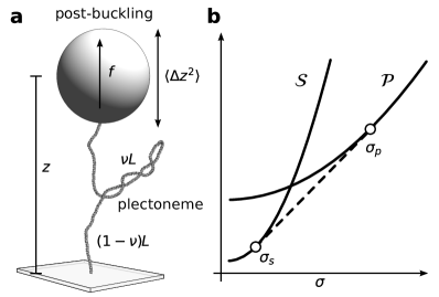
Figure 1: (a) Example of plectoneme supercoil formation as induced in MT experiments by rotation to the end point of a DNA molecule stretched by a linear force $f$. At post-buckling the molecule phase separates into a stretched and a plectonemic phase. The total length of the molecule $L$ is partitioned between the two phases and $0\leq\nu\leq 1$ indicates the fraction of length in the stretched phase. (b) Sketch of free energies per unit length of the stretched and plectonemic phases free energies ${\cal S}$ and ${\cal P}$, respectively, as introduced in the two-phase model of linear supercoiled DNA buckling [5, 6]. The dashed line indicates the double-tangent construction.

Because of its relevance in many biological processes, DNA supercoiling has been attracting significant interest for a long time, both from the experimental and modeling side [5, 6, 7, 8, 9, 10, 11, 12, 13, 14, 15, 16, 17, 18, 19, 20, 21, 22, 23, 24]. The properties of DNA supercoils can be probed in vitro by means of single molecule experiments such as Magnetic Tweezers (MT) [25, 26]. In these experiments a linear DNA molecule is attached to a solid surface at one side and to a paramagnetic bead at the other side (Fig. 1(a)). A magnetic field is used to apply a stretching force $f$ and to control the total torsional strain of the molecule by restricting the rotation of the bead. In a torsionally relaxed DNA, the two strands wind around each other ${Lk}_{0}$ times, corresponding to one turn every $10.5$ base pairs, where ${Lk}$ represents the topological linking number. Rotating the bead away from the relaxed state induces an excess linking number $\Delta{Lk}={Lk}-{Lk}_{0}\neq 0$, which can be either positive or negative for over-wound or under-wound DNA, respectively. It is convenient to define the supercoiling density $\sigma=\Delta{Lk}/{Lk}_{0}$ which is an intensive quantity, independent on the total length of the molecule. Starting from a torsionally relaxed state ($\sigma=0$) under an applied stretching force $f$, one can gradually increase $\sigma$ in a MT experiment. At a certain threshold $\sigma=\sigma_{s}$ the molecule buckles - plectonemic supercoils appear and the end-to-end distance $z$ drops (Fig. 1(a)). Upon further increase of $\sigma$ the plectoneme grows at the cost of the stretched part of the molecule.

Our analysis of linear DNA supercoiling is based on the two-phase model [5, 6] which describes the DNA molecule as being composed of a stretched phase and a plectonemic phase, each with distinct free energies, see Fig. 1(b). In this model, buckling is analogous to a thermodynamic first order transition. While typical theoretical and experimental work on supercoiling in MT focuses on the average signal $\langle z\rangle$, we discuss the fluctuations in the extension $z$ characterized by the variance $\langle\Delta z^{2}\rangle$. Recent experiments show that a change in $\langle\Delta z^{2}\rangle$ can be associated with the formation of topological domains induced by proteins that bridge across different sites of DNA [27]. In addition, insights on equilibrium fluctuations can shed light on the rich dynamics of plectonemes [15].

The aim of this paper is to investigate the properties and origin of fluctuations in linear supercoiled DNA. We first discuss the two state model of DNA supercoiling and extend it to the analysis of fluctuations. We show that the leading contribution to the variance of $z$ are due to phase-exchange fluctuations, i.e. the transient transfer of contour length between the plectonemic and stretched phase. Moreover, our analysis highlights that the extension variance $\langle\Delta z^{2}\rangle$ is a lot more sensitive to the properties of the plectonemic phase than the average extension. It is therefore an excellent quantity to be used for the assessment of plectoneme free energy models [28, 29]. The theoretical analysis is supported by numerical results obtained by extensive Monte Carlo simulations, which are in general good agreement with the two-phase model predictions, both for average quantities and their fluctuations.

II Fluctuations in extension from the two phase model

In order to describe the phenomenology of DNA supercoiling, we follow the commonly employed two-phase model-approach that partitions a DNA molecule of length $L$, stretched by a force $f$ and subject to supercoil density $\sigma$ into two separate phases [5, 6]. A fraction $\nu$ of the entire molecular length is assumed to be in the stretched phase (Fig. 1(a)) maintained at supercoil density $\phi$, while the remainder length is in the plectonemic phase with supercoil density $\psi$. As the total linking number in the system is fixed by the amount of turns applied to the bead (which means that $\sigma$ is fixed), fluctuations of the quantities $\nu$, $\phi$ and $\psi$ are constrained to the requirement for the total linking density to equal the sum of the contributions within the two domains $\sigma=\nu\phi+(1-\nu)\psi$. In the following, we will consider $\nu$ and $\phi$ as independent variables, which fixes $\psi$ to

$$\psi=\frac{\sigma-\nu\phi}{1-\nu}.$$ (1)

Following Ref. [6] we consider the free energies per unit length of the stretched and plectonemic phases ${\cal S}(\phi,f)$ and ${\cal P}(\psi)$, respectively, such that the combined free energy per unit length becomes the linear combination

$${\cal F}(f,\phi,\nu)=\nu{\cal S}(f,\phi)+(1-\nu){\cal P}(\psi).$$ (2)

No explicit force dependence is assumed in ${\cal P}(\psi)$ as plectonemes do not contribute to the end-to-end extension. While specific choices of these free energies will be discussed further on, for the time being we will explore general properties. To reproduce the observed phenomenology we only require the free energies to be convex in $\sigma$ and ${\cal S}(\sigma,f)<{\cal P}(\sigma)$ for small $\sigma$, while ${\cal S}(\sigma,f)>{\cal P}(\sigma)$ for sufficiently large $\sigma$, reflecting the absence of plectonemes at small supercoiling densities and their proliferation at large $\sigma$.

The partition function of a molecule of total length $L$ subject to a stretching force $f$, fixed $\sigma$ and large $L$ is then given by

$$Z(\sigma,f,L)=\int_{0}^{1}d\nu\int_{-\infty}^{+\infty}d\phi\,\,e^{-\beta L{\cal F}(f,\phi,\nu)}\approx e^{-\beta L\widetilde{\cal F}(\sigma,f)},$$ (3)

and where the minimal free energy

$$\widetilde{\cal F}(\sigma,f)\equiv\min_{\{\phi,\nu\}}\left[\nu{\cal S}(\phi,f)+(1-\nu){\cal P}\left(\frac{\sigma-\phi\nu}{1-\nu}\right)\right],$$ (4)

is obtained from the condition of vanishing derivatives $\partial{\cal F}/\partial{\phi}=0$ and $\partial{\cal F}/\partial{\nu}=0$, see [6]. This minimization leads to a double tangent construction (see Fig. 1b)

$$\widetilde{\cal F}(\sigma,f)=\left\{\begin{array}[]{lcc}{\cal S}\left(\sigma,f\right)&&0\leq\sigma\leq\sigma_{s}\\ &&\\ \frac{(\sigma_{p}-\sigma){\cal S}\left(\sigma_{s},f\right)+(\sigma-\sigma_{s}){\cal P}\left(\sigma_{p}\right)}{\sigma_{p}-\sigma_{s}}&&\sigma_{s}\leq\sigma\leq\sigma_{p}\\ &&\\ {\cal P}\left(\sigma\right)&&\sigma\geq\sigma_{p}.\\ \end{array}\right.$$ (5)

In the pre-buckling regime $0\leq\sigma\leq\sigma_{s}$ the minimum corresponds to a pure stretched phase, i.e. $\nu=1$ and $\phi=\sigma$. For $\sigma_{s}\leq\sigma\leq\sigma_{p}$, the free energy is a linear combination of stretched phase and plectoneme phase free energies, with a fraction

$$\nu_{s}=\langle\nu\rangle=\frac{\sigma_{p}-\sigma}{\sigma_{p}-\sigma_{s}},$$ (6)

of molecular contour length contained in the stretched phase. Finally, for $\sigma>\sigma_{p}$, corresponding to $\nu=0$ and $\psi=\sigma$, the plectonemic phase fully engulfs the molecule, reducing the end-point extension to zero. The two-phase model describes buckling as a first order phase transition [6]. For $\sigma_{s}\leq\sigma\leq\sigma_{p}$ the molecule separates into stretched and plectonemic domains with average supercoil densities $\sigma_{s}$ and $\sigma_{p}$ in full analogy to a fluid, which phase-separates into a liquid and a vapor phase with distinct particle densities $n_{L}$ and $n_{V}$. We emphasize that $\sigma_{s}$ and $\sigma_{p}$ are average supercoil densities. At equilibrium, the supercoil densities ($\phi$ and $\psi$) as well as the lengths of the two phases ($\nu$) exhibit fluctuations. It is precisely the scope of this paper to analyze the properties of these equilibrium fluctuations.

The experimentally accessible average molecular extension along the direction of the force director field is obtained from the total derivative of the free energy with respect to the force

$$\frac{\langle z\rangle}{L}=-\frac{d\widetilde{\cal F}}{df},$$ (7)

while the variance is obtained by the second derivative

$$\frac{\langle\Delta z^{2}\rangle}{L}=-k_{B}T\frac{d^{2}\widetilde{\cal F}}{df^{2}}.$$ (8)

II.1 Fluctuations in $\phi$, $\psi$ and $\nu$

The fluctuations of the supercoiling densities $\phi$ and $\psi$ as well as the fractional occupancy of the stretched phase $\nu$ in the post buckling regime can be understood on general grounds. Taylor expansion of the free energy per unit length (2) around the minimum at $\sigma_{s}$ and $\nu_{s}$ yields

$${\cal F}\approx\widetilde{\cal F}+\frac{1}{2}[ {\cal F}_{\nu\nu}(\nu-\nu_{s})^{2}+{\cal F}_{\phi\phi}(\phi-\sigma_{s})^{2}$$

$$+2{\cal F}_{\nu\phi}(\nu-\nu_{s})(\phi-\sigma_{s})],$$ (9)

where $\widetilde{\cal F}$ is the minimal free energy (4) and ${\cal F}_{\nu\nu}$, ${\cal F}_{\phi\phi}$, ${\cal F}_{\phi\nu}$ are the second derivatives of ${\cal F}$ with respect of $\nu$ and $\phi$. These form a $2\times 2$ Hessian matrix, which upon inversion gives the following results for the fluctuations (for details see Appendix A)

$$\langle\Delta\nu^{2}\rangle =\frac{k_{B}T}{L(\sigma_{p}-\sigma_{s})^{2}}\left(\frac{1-\nu_{s}}{{\cal P}_{\psi\psi}}+\frac{\nu_{s}}{{\cal S}_{\phi\phi}}\right),$$ (10)

$$\langle\Delta\phi^{2}\rangle =\frac{k_{B}T}{L\nu_{s}{\cal S}_{\phi\phi}},$$ (11)

$$\langle\Delta\nu\Delta\phi\rangle =\frac{k_{B}T}{L(\sigma_{p}-\sigma_{s}){\cal S}_{\phi\phi}},$$ (12)

where $\Delta\nu\equiv\nu-\nu_{s}$, $\Delta\phi\equiv\phi-\sigma_{s}$ and where ${\cal S}_{\phi\phi}$ and ${\cal P}_{\psi\psi}$ are the second derivatives of the free energies of the stretched and plectonemic phases with respect to the corresponding supercoiling densities. Evaluation at $\phi=\sigma_{s}$ and $\psi=\sigma_{p}$ is implied. Analogously, the plectoneme supercoiling density fluctuates as

$$\langle\Delta\psi^{2}\rangle=\frac{k_{B}T}{L(1-\nu_{s}){\cal P}_{\psi\psi}}.$$ (13)

The variances of the supercoiling densities $\phi$ and $\psi$ are inversely proportional to the curvature of the respective free energy at the minimum, ${\cal S}_{\phi\phi}$ and ${\cal P}_{\psi\psi}$, and the average lengths of the two phases, $\nu_{s}L$ and $(1-\nu_{s})L$. As in the post-buckling regime $\nu_{s}$ decreases with increasing $\sigma$ (Eq. (6)), the variance of the stretched phase supercoil density $\langle\Delta\phi^{2}\rangle$ increases with $\sigma$. Conversely, $\langle\Delta\psi^{2}\rangle$ decreases with increasing $\sigma$, while the cross-correlator $\langle\Delta\nu\Delta\phi\rangle$ is independent on $\sigma$.

In the pre-buckling regime $0\leq\sigma<\sigma_{s}$ the system is in the pure stretched phase $\nu_{s}=1$, such that there are no phase-exchange fluctuations $\langle\Delta\nu^{2}\rangle=0$. When advancing into the post-buckling regime, the system traverses the buckling point where the variance in $\nu$ exhibits a discrete jump into non-zero fluctuations

$$\lim_{\sigma\to\sigma_{s}^{+}}\langle\Delta\nu^{2}\rangle-\lim_{\sigma\to\sigma_{s}^{-}}\langle\Delta\nu^{2}\rangle=\frac{k_{B}T}{L}\frac{1}{{\cal S}_{\phi\phi}(\sigma_{p}-\sigma_{s})^{2}}.$$ (14)

Similarly, fluctuations in $\phi$ and $\psi$ exhibit a discontinuity at the buckling point, since $\phi=\sigma$ and $\psi=0$ at pre-buckling. From Eqs. (10) and (6) we find

$$\frac{d\langle\Delta\nu^{2}\rangle}{d\sigma}=\frac{k_{B}T}{L(\sigma_{p}-\sigma_{s})^{3}}\frac{{\cal S}_{\phi\phi}-{\cal P}_{\psi\psi}}{{\cal S}_{\phi\phi}{\cal P}_{\psi\psi}},$$ (15)

which shows that fluctuations in $\nu$ increase throughout the post-buckling regime if ${\cal S}_{\phi\phi}>{\cal P}_{\psi\psi}$ at the minimum $\phi=\sigma_{s}$, $\psi=\sigma_{p}$. This is the typical behavior of DNA, as the stretched phase is torsionally stiffer than the plectonemic phase [6].

II.2 Quadratic free energies

As a concrete and analytically tractable example we consider quadratic free energies for the two phases [6]

$${\cal S}(\phi,f) = -g(f)+a(f)\phi^{2},$$ (16)

$${\cal P}(\psi) = b\psi^{2}.$$ (17)

While the free energy of the stretched phase of type (16) can be derived from the Twistable Wormlike Chain (TWLC) [30], the form of the plectonemic free energy (17) is purely phenomenological. It assumes symmetry in $\pm\psi$, valid at low forces ($f<1$ pN) where the DNA has an almost symmetric behavior upon over- and under-winding. Eq. (17) can be viewed as the lowest order expansion of a generic ${\cal P}(\psi)$. As such, this form will be valid for sufficiently small supercoiling densities. For the TWLC the coefficients $g$ and $a$ describing the free energy of the stretched phase are force-dependent [31, 30, 32]. Since the system is assumed to be fully in the stretched phase at low supercoiling densities, we require $g>0$ to ensure that ${\cal S}(0,f)<{\cal P}(0)$. Moreover, to have a transition from stretched to plectonemic phase, the free energy of the former has to exceed that of the latter (${\cal P}<{\cal S}$) for sufficiently large supercoiling density, which requires $a(f)>b$ (this corresponds to ${\cal S}_{\phi\phi}>{\cal P}_{\psi\psi}$, i.e. an increase in variance with increasing $\sigma$, as per Eq. (15)).

For the free energies (16) and (17) the double tangent construction yields the average supercoiling densities of stretched and plectonemic phases [6]

$$\langle\phi\rangle=\sigma_{s}=\sqrt{\frac{bg}{a(a-b)}}, \langle\psi\rangle=\sigma_{p}=\sqrt{\frac{ag}{b(a-b)}}.$$ (18)

The free energy in the post-buckling regime ($\sigma_{s}\leq\sigma\leq\sigma_{p}$) assumes the form

$$\widetilde{\cal F}(\sigma,f)=-\frac{ga}{a-b}+2\sigma\sqrt{\frac{gab}{a-b}},$$ (19)

which is linear in $\sigma$ and depends on $f$ through the force-dependence of $g$ and $a$.

As ${\cal S}_{\phi\phi}=2a$ and ${\cal P}_{\psi\psi}=2b$, the fluctuations of Eqs. (10)-(13) take the form

$$\langle\Delta\nu^{2}\rangle = \frac{k_{B}T\sigma}{2Lg^{3/2}}\,\sqrt{\frac{ab}{a-b}},$$ (20)

$$\langle\Delta\phi^{2}\rangle = \frac{k_{B}T}{2aL\nu_{s}},$$ (21)

$$\langle\Delta\psi^{2}\rangle = \frac{k_{B}T}{2bL(1-\nu_{s})},$$ (22)

$$\langle\Delta\phi\Delta\nu\rangle = \frac{k_{B}T}{2L}\sqrt{\frac{ab}{g(a-b)}},$$ (23)

where we used (18). Note that $\langle\Delta\nu^{2}\rangle$ increases with $\sigma$, as deduced from (15): the stretched phase is torsionally stiffer than the plectonemic phase ($a>b$).

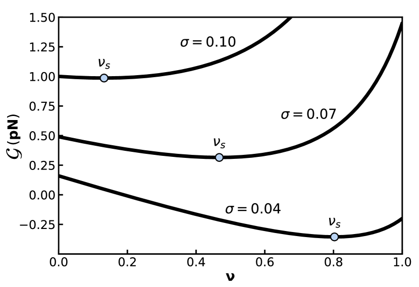
Figure 2: Plot of ${\cal G}(\nu)$ the free energy per unit length (25) vs. $\nu$, the fraction of length in the stretched phase. As $\sigma$ increases the minimum $\nu_{s}=\langle\nu\rangle$ shifts towards $\nu=0$, the pure plectonemic phase. Fluctuations $\langle\Delta\nu^{2}\rangle$ are determined by the curvature around the minimum ${\cal G^{\prime\prime}}(\nu_{s})$, as given in Eq. (20). The curvature decreases with increasing $\sigma$, implying an increase of fluctuations with $\sigma$. These curves correspond to $g=1$ pN, $a=500$ pN and $b=100$ pN (${\cal G}$ is a free energy per unit of length, which means that it has the dimension of a force and is therefore expressed in units of pN).

While so far we have considered the asymptotic limit $L\to\infty$, one can extend the analysis to finite length effects. For this purpose one can start from (3) and perform the (Gaussian) integral on $\phi$ explicitly

$$Z(\sigma,f,L) = \int_{0}^{1}d\nu\int_{-\infty}^{+\infty}d\phi\,\,e^{-\beta L\nu{\cal S}(\phi,f)}e^{-\beta L(1-\nu){\cal P}(\psi)}$$ (24)

$$= \ldots\int_{0}^{1}d\nu\,e^{-\beta L{\cal G}(\nu)},$$

where the dots indicate subleading terms in $1/L$. The free energy ${\cal G}(\nu)$ is found to be

$${\cal G}(\nu)=-\nu g+\Xi(\nu)\,\sigma^{2},$$ (25)

which is characterized by an effective stiffness

$$\frac{1}{\Xi(\nu)}=\frac{\nu}{a}+\frac{1-\nu}{b},$$ (26)

given by the weighted harmonic mean of the stiffnesses of the stretched ($a$) and plectonemic ($b$) phases. As expected this free energy reduces to the pure state free energies in the two extremal cases ${\cal G}(\nu=1)={\cal S}$ and ${\cal G}(\nu=0)={\cal P}$. ${\cal G}(\nu)$ is plotted in Fig. 2 for three different values of $\sigma$. In the post-buckling regime $\sigma_{s}<\sigma<\sigma_{p}$ the fluctuations of $\nu$ are obtained from the second derivative of ${\cal G}(\nu)$ calculated in $\nu_{s}$ from which one recovers (20). This Gaussian approximation is valid at large $L$ and breaks down in the vicinity of the phase boundaries $\nu_{s}\approx 0$ and $\nu_{s}\approx 1$. In that case the partition function (24) can be obtained by numerical integration.

II.2.1 Rigid rod model

To highlight the phenomenology of the extension fluctuations we start with a simple model in which thermally activated bending fluctuations within stretched phase are neglected. We assume that this phase consists of twistable rigid rods aligned along the direction of the force. This corresponds to setting $g(f)=f$ and $a(f)=a$ in Eq. (16), with $a$ constant. In the pre-buckling regime $0<\sigma<\sigma_{s}$ one obtains average and variance of $z$ from differentiating ${\cal S}(\sigma,f)$ with respect to $f$. The calculation gives $\langle z\rangle=L$ and $\langle\Delta z^{2}\rangle=0$, showing that this choice of stretched phase free energy indeed represents a straight rod. In the post-buckling regime $\sigma_{s}<\sigma<\sigma_{p}$ differentiation of (19) is simple as the only force dependence in the parameters is $g=f$

$$\frac{\langle z\rangle}{L}=-\frac{d\widetilde{\cal F}}{df}=\frac{a}{a-b}-\frac{\sigma}{\sqrt{f}}\sqrt{\frac{ab}{a-b}}.$$ (27)

Using (18) one can easily verify that (27) yields $\langle z\rangle=L$ for $\sigma=\sigma_{s}$ and that $\langle z\rangle=0$ for $\sigma=\sigma_{p}$. For the variance one obtains

$$\frac{\langle\Delta z^{2}\rangle}{L}=-k_{B}T\frac{d^{2}\widetilde{\cal F}}{df^{2}}=\frac{k_{B}T\sigma}{2f^{3/2}}\sqrt{\frac{ab}{a-b}}=L\langle\Delta\nu^{2}\rangle,$$ (28)

where the last equality follows from (20). As the stretched phase does not exhibit extension fluctuations, the only source for fluctuations in $z$ stems from the exchange of contour length between the two phases (fluctuations of $\nu$). We note that the relation

$$\langle\Delta z^{2}\rangle=L^{2}\langle\Delta\nu^{2}\rangle,$$ (29)

follows directly from the observation that the variance of $\nu$ can be obtained from the second derivative of the free energy in $g$. This is because $g$ and $\nu$ enter in the Boltzmann factor of (24) in the combination $g\nu$.

II.2.2 Twistable worm-like chain (TWLC)

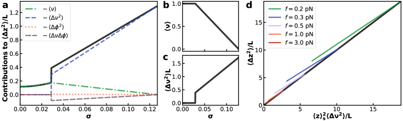
Figure 3: (a) Plot of the total extension variance $\langle\Delta z^{2}\rangle$ vs. $\sigma$ (solid line) and of the four different terms (dashed, dotted and dashed-dotted colored lines) on the right hand side of Eq. (32) with the force set to $f=2$ pN. The sum of these terms gives $\langle\Delta z^{2}\rangle$. The plot shows that the leading contribution to $\langle\Delta z^{2}\rangle$ is due to the length exchange fluctuations, i.e. the term proportional to $\langle\Delta\nu^{2}\rangle$. (b) Plots of $\langle\nu\rangle$ and (c) $\langle\Delta\nu^{2}\rangle$ vs. $\sigma$ for $f=2$ pN. The former decreases linearly in $\sigma$ (6), while the latter is discontinuous at the buckling point (14), followed by a linear increase throughout the post-buckling regime (20). (d) The colored lines are plots of $\langle\Delta z^{2}\rangle$ vs. $\langle z\rangle_{\cal S}^{2}\,\langle\Delta\nu^{2}\rangle$ testing (36) for different forces and $\sigma_{s}\leq\sigma\leq\sigma_{p}$. The black line is the diagonal $x=y$ indicating perfect agreement between the two quantities. For the calculations reported in these plots we used $A=40$ nm, $C=100$ nm, $P=20$ nm and $\omega_{0}=1.76\,\text{nm}^{-1}$ (corresponding to one one full turn of the helix each 10.5 base pairs).

To account for the effect of bending fluctuations, we invoke the twistable worm-like chain (TWLC) [10, 33, 34, 35]. In this model DNA is represented as an inextensible continuous twistable rod with an associated bending stiffness $A$ and twist stiffness $C$. The behavior of the TWLC within the extended phase has been studies for both small [36, 37] and large forces [31, 30, 32]. Here we use the high force expansion of the stretched phase free energy, which is given by Eq. (16) with

$$g(f) = f\left(1-\sqrt{\frac{k_{B}T}{Af}}+\ldots\right),$$ (30)

$$a(f) = \frac{C}{2}\left(1-\frac{C}{4A}\sqrt{\frac{k_{B}T}{Af}}+\ldots\right)k_{B}T\omega_{0}^{2},$$ (31)

where $\omega_{0}\approx 1.76$ nm^-1 is the intrinsic helical twist of DNA. Note, that in the limit $A\to\infty$, which amounts to suppressing bending fluctuations, one recovers the rigid rod model of section II.2.1.

Without making any particular choice for the plectoneme free energy ${\cal P}$, the extension variance $z$ can be expressed in terms of the fluctuations of $\nu$ and $\phi$. Double differentiation of the post-buckling free energy (19) in $f$, see Eq. (8), leads to the relation (details of in Appendix B)

$$\langle\Delta z^{2}\rangle = k_{B}TL\langle\nu\rangle(g_{f\!f}-a_{f\!f}\sigma_{s}^{2})$$ (32)

$$+ L^{2}\left[\left(g_{f}-a_{f}\sigma_{s}^{2}\right)^{2}\langle\Delta\nu^{2}\rangle+4a_{f}^{2}\langle\nu\rangle^{2}\sigma_{s}^{2}\langle\Delta\phi^{2}\rangle\right.$$

$$- 4a_{f}\left.\langle\nu\rangle\sigma_{s}\left(g_{f}-a_{f}\sigma_{s}^{2}\right)\langle\Delta\nu\Delta\phi\rangle\right],$$

where we omitted higher than second order cumulants and adopted the shorthand notation $g_{f}\equiv dg/df$ and $g_{f\!f}\equiv d^{2}g/df^{2}$. The correlators $\langle\Delta\nu^{2}\rangle$, $\langle\Delta\phi^{2}\rangle$ and $\langle\Delta\nu\Delta\phi\rangle$ scale as $1/L$, see Eqs. (20)-(22), while $\langle\nu\rangle$ is independent of $L$, such that all the terms on the right hand side of (32) scale as $L$, i.e. they retain their relevance for large $L$. Note that (32) reduces to (29) in the rigid rod limit $g_{f}=1$ and $a_{f}=a_{f\!f}=g_{f\!f}=0$.

Eq. (32) decomposes $\langle\Delta z^{2}\rangle$ into contributions stemming from different fluctuating quantities. For example, the innate stretched phase variance $\langle\Delta z^{2}\rangle$ for a domain of length $L_{s}$ with supercoiling density $\sigma_{s}$ is

$$\langle\Delta z^{2}\rangle_{\cal S}=-k_{B}TL_{s}\frac{d^{2}{\cal S}}{df^{2}}=k_{B}TL_{s}(g_{f\!f}-a_{f\!f}\sigma^{2}).$$ (33)

At mean fractional occupancy $\langle\nu\rangle$ this domain length is $L_{s}=\langle\nu\rangle L$, which yields the first term in Eq. (32).

Evaluation of the remaining contribution requires the calculation of the correlators, which depend on the specific functional form of the plectoneme free energy ${\cal P}$. Following prior work [6, 38] we invoke the harmonic form (17) with the conventional parametrization [6]

$$b=\frac{1}{2}Pk_{B}T\omega_{0}^{2},$$ (34)

where $P$ is usually referred to as the effective torsional stiffness of the plectonmic phase [38], which like $A$ and $C$ is expressed in units of length. A plot of $\langle\Delta z^{2}\rangle$, as well as the four different contributions on the right hand side of Eq. (32), in function of $\sigma$ for $f=2.0$ pN are shown in Fig. 3(a). In the pre-buckling regime, the stretched phase fully occupies the chain such that $\nu=1$ and $\phi=\sigma$ remain constant, leaving Eq. (33) with $L_{s}=L$ as the only non-zero contribution to $\langle\Delta z^{2}\rangle$. This contribution decreases linearly in $\sigma$ in the post-buckling regime, reflecting the decrease of $\langle\nu\rangle$ with $\sigma$. Generally, as a consequence of the linear dependence of the free energy (19) on $\sigma$ in this regime, all four contributions to $\langle\Delta z^{2}\rangle$ scale linearly with $\sigma$. We note that the term proportional to $\langle\Delta\phi^{2}\rangle$ (orange dotted line in Fig. 3(b)) provides a very small contribution to $\langle\Delta z^{2}\rangle$. The term proportional to the mixed correlator $\langle\Delta\nu\Delta\phi\rangle$ gives an overall negative contribution to $\langle\Delta z^{2}\rangle$, partially canceling the contribution of the stretched phase fluctuations proportional to $\langle\nu\rangle$.

The analysis of Fig. 3(b) shows that the leading contribution to $\langle\Delta z^{2}\rangle$ comes from the term proportional to the phase-exchange fluctuations $\langle\Delta\nu^{2}\rangle$. We can rewrite this term by using the force-extension relation for the stretched phase at supercoiled density $\sigma$

$$\frac{\langle z\rangle_{\cal S}}{L}=-\frac{d{\cal S}}{df}=g_{f}-a_{f}\sigma^{2}.$$ (35)

Using this we can then write for the leading contribution to the variance of $z$ as

$$\langle\Delta z^{2}\rangle\approx\langle z\rangle_{\cal S}^{2}\,\langle\Delta\nu^{2}\rangle,$$ (36)

where $\langle z\rangle_{\cal S}$ is computed at $\sigma_{s}$. Figure 3(c) shows a plot of $\langle\Delta z^{2}\rangle$ vs. $\langle z\rangle_{\cal S}^{2}\,\langle\Delta\nu^{2}\rangle$ for different forces and $\sigma_{s}\leq\sigma\leq\sigma_{p}$ indicating good agreement between the two terms.

III Twistable Worm-like chain Monte Carlo

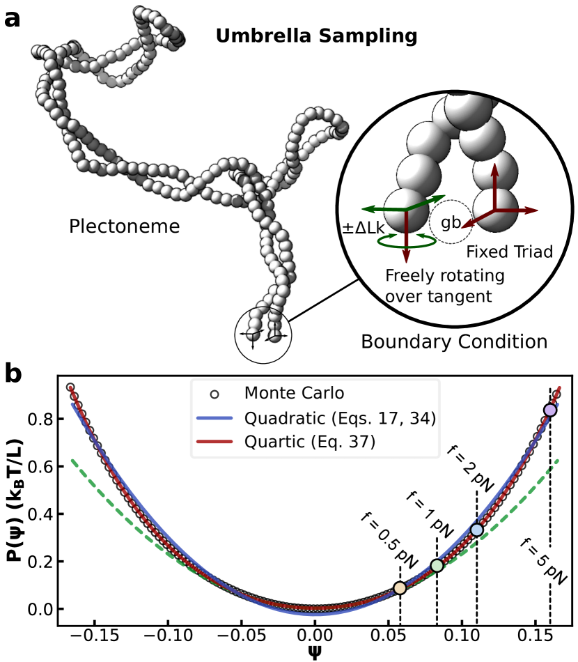
Figure 4: (a) Snapshot of MC simulation used to calculate the free energy of the plectonemic phase ${\cal P}(\psi)$, via umbrella sampling. The first and last beads are maintained fixed in space $8$ nm apart, with an antiparallel orientation of their local tangents. The triad attached to the first bead is fully prevented from rotating and that attached to the last bead is only permitted to rotate freely about its tangent, allowing for diffusion of torsional strain into and out of the system. Between these boundary beads we place demobilized ghost-bead (gb) to prevent any part of the molecule to cross through the open gap. By initializing each simulation with zero linking number, the linking number at any snapshot is given by the accumulative rotation angle of the last triad. High supercoiling densities $\sigma$ are induced by introducing biasing torques. We perform simulations for torques ranging from $1$ to $30$ pN$\cdot$nm spaced in integer steps. For each torque we sample $10^{7}$ independent configuration for a total of $3\times 10^{11}$ Monte Carlo steps. (b) Monte Carlo sampled free energy (circles) and approximations with quadratic and quartic models. Best agreement with the quadratic model Eq. (34) is found for $P=20.5$ nm (solid blue line). Considering the quartic model Eq.(37) with $P_{2}=14.4$ nm and $P_{4}=524.04$ nm (solid red line) improves the agreement with the MC free energy. The quadratic free energy with $P=P_{2}$ is indicated with a green dashed line. The dashed vertical lines indicate the estimated values of $\sigma_{p}$ (the average $\langle\psi\rangle$) for four different forces. Our umbrella sampling simulations are similar to those of Ref. [8] performed on a different coarse-grained model of DNA. Deviations from harmonic behavior were already noted yet not quantified in that work.

We tested the predictions of the two-phase model by means of Monte Carlo (MC) simulations of the dicrete Twistable Wormlike Chain (TWLC), see e.g. [27]. The discrete TWLC consists of a series of spherical beads carrying each an orthonormal triad of unit vectors (Fig. 4a). In our simulations each coarse-grained bead corresponds to $10$ base pairs of DNA. From the relative orientations between two consecutive triads we compute bending and twist angles. The TWLC bending and twist energy is calculated from the bending and torsional stiffnesses given by the two parameters $A$ and $C$, respectively. Following Rybenkov et al. [39] we account for both salt-concentration dependent electrostatic repulsion as well as steric self-avoidance by hard spheres with an effective diameter $d_{EV}$ that exceeds the physical extension of the underlying molecule. Throughout this work we use $d_{EV}=4.0$ nm, $A=40$ nm and $C=100$ nm, which were shown to produce the best agreement with magnetic tweezers measurements in a buffer of $150$ mM univalent salt [27]. Further details on the simulation protocol can be found in supplemental material of Ref. [27].

III.1 Plectoneme Free Energy

In a first step we utilize the MC simulations to explore the free energy of the plectonemic phase ${\cal P}(\psi)$ by umbrella sampling [40]. With appropriately imposed boundary conditions, we restrict simulations of chains of length $L=680$ nm ($2$ kbp) to the plectonemic phase (see Fig. 4b and caption for details) and repeat the simulation for a range of biasing torques to sample supercoiling densities $\psi$ in the range of $-0.165\leq\psi\leq 0.165$. We employ WHAM (Weighted Histogram Analysis Method) [41] to construct a single unbiased histogram that combines all individual biased histograms in $\psi$. Boltzmann-inversion then yields the sought plectoneme free energy ${\cal P}(\psi)$, see Fig. 4a. The best fit for the effective torsional stiffness of the plectonemic state for the quadratic model ${\cal P}=b\psi^{2}$ (with the parametrization of Eq. (34)) over the entire sampled range is found to be $P=20.5$ nm, which is consistent with previous experimental measurements [38, 27]. However, closer inspection shows that MC data deviate from the quadratic model free energy. Instead, the quartic functional form

$${\cal P}(\psi)=\left(\frac{P_{2}}{2}\psi^{2}+\frac{P_{4}}{4}\psi^{4}\right)\omega_{0}^{2}k_{B}T,$$ (37)

is found to agree significantly better with the sampled energy. As the supercoiling density $\psi$ is dimensionless, both $P_{4}$ and $P_{2}$ have the unit of a length. Smallest least squared differences are attained for the coefficients $P_{2}=14.4$ nm and $P_{4}=524.04$ nm. For $\psi<0.075$ the relative contribution of the quartic term is less than $10\%$ (and less than $5\%$ for $\psi<0.05$), suggesting the quadratic model to be a reasonable approximation in this regime, albeit with a stiffness of $P_{2}$, which is about $25\%$ lower than the consensus values reported in the literature [38, 27]. We note that deviations from the quadratic behavior become more relevant at high tension as in this regime the average supercoil density of the plectonemic phase $\sigma_{p}=\langle\psi\rangle$ becomes larger ($\sigma_{s}$ and $\sigma_{p}$ grow with $f$, see Eqs. (18) and recall that $g\sim f$). In the high tension post-buckling regime, it becomes important to include the quartic term. The vertical dashed lines in Fig. 4b show the values of $\sigma_{p}$ for four different forces.

It is important to note that the double tangent construction (Eq. 5) is determined not only by the free energies ${\cal S}(\phi,f)$ and ${\cal P}(\psi)$, but also their local derivatives. While the global quadratic fit of the free energy may appear to be a reasonable approximation for ${\cal P}$ over the full range of $\psi$, the quartic term is necessary for a good approximation of the free energy derivatives ${\cal P}_{\psi}$ and ${\cal P}_{\psi\psi}$ (the latter contributes to the variances (10) and (13)).

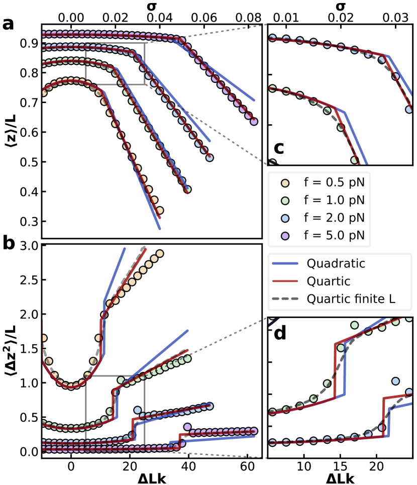
Figure 5: Rotation curves of (a) extension and (b) extension variance in function of applied turns ($\Delta{Lk}$ or $\sigma$) for 4 different stretching forces ($0.5$ pN, $1$ pN, $2$ pN and $5$ pN). Colored markers show $\langle z\rangle$ and $\langle\Delta z^{2}\rangle$ for Monte Carlo simulations of the TWLC for a molecule of length $L=2692.8$ nm ($7920$ bp). For each combination of force and linking density we performed $10^{11}$ Monte Carlo steps sampling the extension every $100$ steps. Solid blue lines give the respective values for the two-phase model with quadratic plectoneme free energy ${\cal P}$ using $P=20.5$ nm. Two-phase model curves with quartic ${\cal P}$ using $P_{2}=14.4$ nm and $P_{4}=524.04$ nm are shown as solid red lines. Grey solid lines show the a numerical integration of the two-phase model with quartic free energy. Panels (c) and (d) show a zoom-in on the buckling transition for $\langle z\rangle$ and $\langle\Delta z^{2}\rangle$, respectively. The finite length numerical calculation, with $L$ matching the chain length considered in the Monte Carlo simulations, is indicated by the grey dashed line.

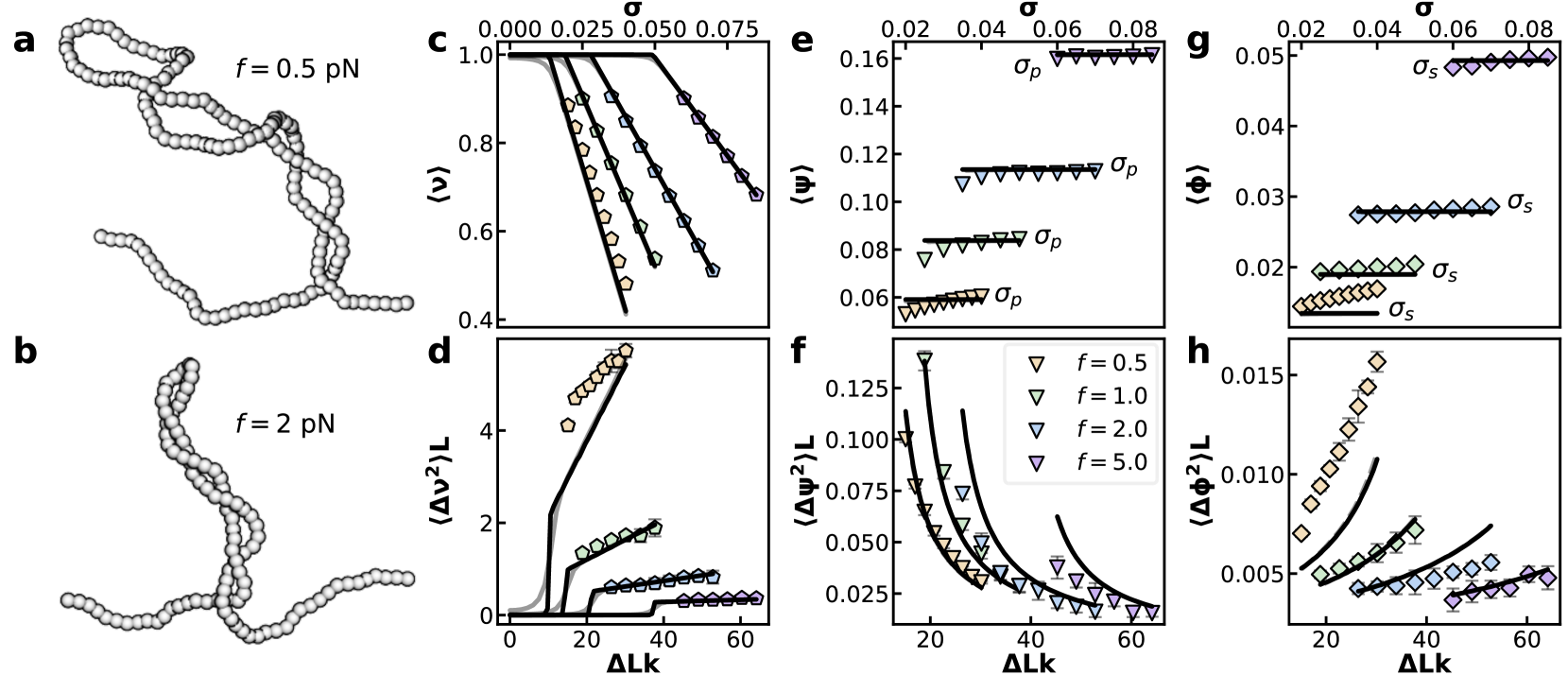
Figure 6: (a,b) Snapshots of MC simulations for two different forces. At higher tension (b) the plectoneme is considerably tighter than at lower tension (a) which is reflected by a significantly larger supercoiling density $\sigma_{p}$. Using a plectoneme-detecting algorithm (Appendix C) we have computed averages and variances of the fraction of length in the straight phase $\nu$ (c, d), and the supercoiling density of the plectonemic phase $\psi$ (e, f) and of the straight phase $\phi$ (g, h). Solid lines in c-g are the predictions of the two-phase model, using the quartic free energy for the plectonemic phase (37) and the expansion (38) for $g(f)$.

III.2 The mean extension and the extension variance

Next, we consider linear DNA molecules of length $L=2692.8$ nm ($7920$ bp), subject to different stretching forces ($0.5$ to $5$ pN). We performed Monte Carlo simulations in the fixed linking number ensemble within a range of relevant supercoiling densities. From the sampled ensembles we obtain data of mean extension $\langle z\rangle$ (Fig. 5a) and extension variance $\langle\Delta z^{2}\rangle$ (Fig. 5b), which we compare to the predictions of the two-phase model. For the stretched phase free energy we use Eq. (16) with $g(f)$ and $a(f)$ defined by Eqs. (30) and (31). We include the next higher order term in the expansion of $g$

$$g(f)=f\left(1-\sqrt{\frac{k_{B}T}{Af}}+g_{2}\frac{k_{B}T}{Af}\right).$$ (38)

Using the numerically exact solution of a stretched Wormlike Chain [31] we find $g_{2}=0.3$ for $A=40$ nm, and the room temperature value $k_{B}T=4.1$ pN$\cdot$nm. The term proportional to $g_{2}$ contributes as an overall force-independent constant to the stretched phase free energy, and thus does not modify the statistical properties of this phase. However, $g_{2}$ is relevant in the double tangent construction as it gives a constant relative shift to the stretched and plectoneme phase free energies.

The quadratic free energy two-phase model as defined in Eq. (34) using the umbrella sampled full range optimization $P=20.5$ nm yields reasonable agreement with the MC sampled mean extension $\langle z\rangle$, albeit with visible deviations in the post-buckling slopes. As anticipated in the discussion of the free energy, the most substantial deviations are observed for large forces. Large forces imply tight plectonemic coiling (large $\langle\psi\rangle=\sigma_{p}$), where the deviation of ${\cal P}$ from the quadratic model are most notable, see Fig. 4a. The deviations between theory and simulations are almost entirely resolved by invoking the quartic model (37), which yields excellent agreement with the mean extension of the MC data across the full range of forces.

In spite of the success of the quartic model for the mean extension, the variance reveals the existence of remnant shortcomings. While the general features are quite accurately reproduced and the high force agreement is rather convincing, the slope of the low force variance significantly overestimates the MC data. Nonetheless, the quartic free energy constitutes a compelling improvement to the quadratic model.

We also performed a numerical integration of the full partition function. This reveals finite $L$ effects that are not captured by the free energy minimization approach (3), which is valid in the thermodynamic limit. The difference between the two calculations is mostly visible in the vicinity of the phase boundary $\sigma=\sigma_{s}$ (see Fig. 5c,d). Here the Gaussian approximation predicts a jump of $\langle\Delta z^{2}\rangle$, while the numerical integration smoothly connects the pre- and post-buckling regimes, and matches the simulation data in the pre-buckling regime.

III.3 Two-phase model degrees of freedom

Inspired by previous work [9, 42, 43], we developed an algorithm to detect the regions occupied by the plectonemic phase in simulation generated snapshots (see Appendix C for details). With this algorithm we calculated the total fraction of stretched phase $\nu$, and the supercoiling densities of the stretched and plectonemic phases, $\phi$ and $\psi$. We compared these results with the prediction of the two-phase model, employing the quartic model (Eq. (37)) for the plectoneme free energy with the parameters obtained from umbrella sampling. The averages $\langle\nu\rangle$, $\langle\psi\rangle$ and $\langle\phi\rangle$ convincingly follow the prediction of the two-phase model, at least for large forces (Figs. 6a, c and e). We note that $\langle\nu\rangle$ is linear in $\sigma$, as expected from Eq. (6). Moreover, $\langle\phi\rangle=\sigma_{s}$ and $\langle\psi\rangle=\sigma_{p}$ are approximately independent of $\sigma$. Deviations are apparent for the smallest force ($0.5$ pN) and close to the buckling point $\sigma\approx\sigma_{p}$, where finite length effects are of relevance. The variances $\langle\Delta\nu^{2}\rangle$, $\langle\Delta\psi^{2}\rangle$ and $\langle\Delta\phi^{2}\rangle$ show stronger deviations from the theory as compared to the averages, especially at the smallest force analyzed $f=0.5$ pN. Considering the inherent difficulty to determine phase-boundaries, and the sensitivity of higher moments to algorithmic noise, we observe satisfactory agreement between theory and simulations for the variances of $\nu$, $\psi$ and $\phi$ (Figs. 6(b),(d) and (f)). For all forces the two-phase model theory qualitatively captures the general trends of the fluctuations. Quantitative agreement is once again limited to the higher force regime $f\gtrsim 1$ pN.

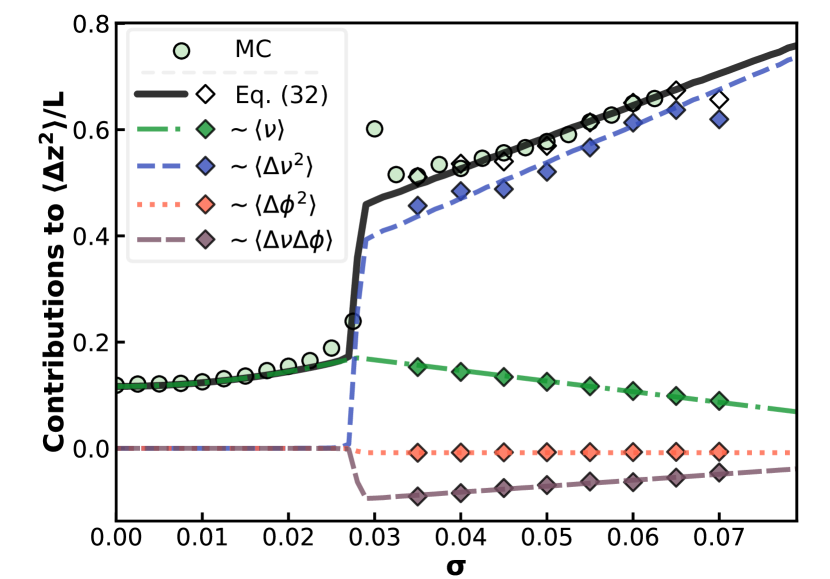
Figure 7: Comparison of the extension variance $\langle\Delta z^{2}\rangle$ for $f=2$ pN (black solid line: theory with quartic ${\cal P}$; round symbols: TWLC MC) to the four different contributions according to Eq. (32) (blue: term $\sim\langle\Delta\nu^{2}\rangle$; green: term $\sim\langle\nu\rangle$; orange: term $\sim\langle\Delta\phi^{2}\rangle$; brown: term $\sim\langle\Delta\nu\Delta\phi\rangle$). The numerical calculations with quartic ${\cal P}$ are shown as lines and MC data as diamonds. White diamonds represent the sum of the MC extracted contributions.

III.4 Contributions to extension variance

Finally, we verify if the conclusions of Section II.2.2 that were obtained for the two-phase model with quadratic free energies still hold for a quartic plectoneme free energy and for the TWLC Monte Carlo simulations. The expectation values for $\langle\nu\rangle$, $\langle\Delta\nu^{2}\rangle$, $\langle\Delta\phi^{2}\rangle$ and $\langle\Delta\nu\Delta\phi\rangle$, calculated numerically for the for quartic ${\cal P}$ and deduced from TWLC Monte Carlo simulations as shown in Fig. 6, allow us to once again decompose the extension variance into various contributions according to Eq. (32). Note, that this equation remains valid as long as the stretched phase free energy is reasonably well approximated by the stretching free energy (30) and twist free energy (31). Given the excellent agreement between the theoretical and simulated $\langle z\rangle$ and $\langle\Delta z^{2}\rangle$ in the pre-buckling regime (see Fig. 5) we consider this requirement satisfied. The differences between the quadratic and quartic ${\cal P}$ are fully contained in the the correlators (see Eq. (32)).

In Fig. 7 the extension variance of the TWLC Monte Carlo simulations for $f=2$ pN is compared to the contributions stemming from $\langle\nu\rangle$, $\langle\Delta\nu^{2}\rangle$, $\langle\Delta\phi^{2}\rangle$ and $\langle\Delta\nu\Delta\phi\rangle$ according to Eq. (32). Just as in the case of the quadratic free energy, the extension variance $\langle\Delta z^{2}\rangle$ is dominated by phase exchange fluctuations $\langle\Delta\nu^{2}\rangle$, especially for large supercoiling densities, where the system shows a significant occupancy of the plectonemic phase.

IV Conclusion

In this paper we discussed the properties of end-point fluctuations of linear stretched and overtwisted DNA. This is the typical setup of single molecule MT experiments in which a magnetic field is used to apply a stretching force $f$ and to maintain kbp-long DNA molecule at fixed linking number. We based our analysis on a two-phase model [6], which describes DNA buckling as a thermodynamic first order transition.

In the pre-buckling regime, both mean extension $\langle z\rangle$ as well as extension fluctuations, characterized by the variance $\langle\Delta z^{2}\rangle$, are controlled by the behavior of the stretched phase. Past the buckling point, the DNA consists of coexisting stretched and plectonemic domains. The average length of the plectonemic phase increases with increasing supercoiling density $\sigma$, while the stretched phase decreases, leading to a global decrease of $\langle z\rangle$. The two-phase model indicates that several terms contribute to $\langle\Delta z^{2}\rangle$, representing distinct fluctuation mechanisms, see Eq. (32). While $\langle\Delta z^{2}\rangle$ linearly increases with $\sigma$ at post-buckling, the contribution of extension fluctuations of the stretched phase (term proportional to $\nu$ in (32)) decreases, as this phase decreases in length. We show that of all the contributions to $\langle\Delta z^{2}\rangle$, phase-exchange fluctuations, e.g. the transient exchange of lengths between the stretched and the plectonemic phases through which the plectonemes shrink and grow, is the dominant one. Equation (36), which approximates (32), summarizes the dominance of the length exchange mechanism. The remaining contributions to the extension variance $\langle\Delta z^{2}\rangle$ are due to fluctuations of the supercoiling densities of the stretched and plectonemic phases and of mixed terms coupling stretched phase length and supercoiling density. Although the overall contribution of these terms to $\langle\Delta z^{2}\rangle$ is minor, we note a perhaps curious cancellation between a (positive) stretched phase fluctuation term and a (negative) mixed correlator term. These two contributions are indicated as $\sim\langle\nu\rangle$ and $\sim\langle\Delta\phi\Delta\nu\rangle$ in Figs. 3a and 7. The contribution to $\langle\Delta z^{2}\rangle$ due to the fluctuations of stretched phase supercoil density (term indicated with $\sim\langle\Delta\phi^{2}\rangle$ in Figs. 3a and 7) is generally small.

We corroborate these theoretical predictions with Monte Carlo simulations of the discrete TWLC. In a first step we ascertain the most appropriate form for the plectonemic free energy ${\cal P}$ by umbrella sampling. We find that the quadratic free energy (17) is a good approximation only for plectoneme supercoiling densities $\sigma_{p}$ smaller than roughly $0.05$. Beyond that, the quartic (37) is found to yield satisfactory agreement. For large forces, the use of the quartic ${\cal P}$ is found to significantly increase the agreement between theoretical extension and extension variance curves and Monte Carlo sampled data as compared to the previously used quadratic [6, 27]. Our analysis suggests that the two-phase model captures the phenomenology of the fluctuations in the post-buckling regime. Discrepancies observed at small forces ($f\leq 1$ pN) are likely due to a breakdown of a two-phase model description. At small forces, both plectonemes and stretched parts are loose and are likely to be separated by a smooth and extended interfacial region. This leads to a difficulty in sharply separating plectonemes from stretched domains. In spite of these deviations, the overall qualitative picture holds also at small forces.

Summarizing, we believe that an in-depth understanding of the nature of equilibrium fluctuations of stretched supercoiled DNA is important, since in the cell, as well as in in-vitro experiments, DNA subject to strong thermal fluctuations. Moreover, fluctuations can carry information about processes that do not affect average quantities, as was illustrated in a recent study of protein binding on supercoiling DNA [27].

Appendix A Gaussian fluctuations of $\nu$ and $\phi$

Here, we provide additional details on the calculations of the fluctuations in $\nu$, $\phi$ and $\psi$ given in Eqs. (10), (11), (12) and (13). We use the same notation as in the main text: subscripts denote differentiation with respect to the indicated variable followed by evaluation at the minimum. For example

$${\cal P}_{\psi}=\left.\frac{d{\cal P}}{d\psi}\right|_{\psi=\sigma_{p}}, \psi_{\nu}=\left.\frac{d\psi}{d\nu}\right|_{\phi=\sigma_{s},\nu=\nu_{s}}.$$ (39)

Using the expression for the free energy (2) we find for the second derivative in $\nu$

$${\cal F}_{\nu\nu} = -2{\cal P}_{\psi}\psi_{\nu}+(1-\nu_{s})\left({\cal P}_{\psi}\psi_{\nu\nu}+{\cal P}_{\psi\psi}\psi_{\nu}^{2}\right)$$ (40)

$$= (1-\nu_{s}){\cal P}_{\psi\psi}\psi_{\nu}^{2}=\frac{(\sigma_{p}-\sigma_{s})^{2}}{1-\nu_{s}}{\cal P}_{\psi\psi},$$

where we have used the following relations

$$\psi = \frac{\sigma-\phi}{1-\nu}-\phi,$$ (41)

$$\psi_{\nu} = \frac{\sigma-\sigma_{s}}{(1-\nu_{s})^{2}}=\frac{\sigma_{p}-\sigma_{s}}{1-\nu_{s}},$$ (42)

$$\psi_{\nu\nu} = 2\frac{\sigma-\sigma_{s}}{(1-\nu_{s})^{3}}=\frac{2\psi_{\nu}}{1-\nu_{s}}.$$ (43)

Likewise, we find for the other derivatives

$${\cal F}_{\phi\phi} =\frac{\nu_{s}}{1-\nu_{s}}\left[(1-\nu_{s}){\cal S}_{\phi\phi}+\nu_{s}{\cal P}_{\psi\psi}\right],$$ (44)

$${\cal F}_{\phi\nu} =\frac{\nu_{s}}{1-\nu_{s}}(\sigma_{p}-\sigma_{s}){\cal P}_{\psi\psi}.$$ (45)

Equipartition then stipulates that fluctuations in $\phi$ and $\nu$ are obtained from the inversion of the Hessian matrix. This gives

$$\beta L\langle\Delta\nu^{2}\rangle=\frac{{\cal F}_{\phi\phi}}{{\cal F}_{\nu\nu}{\cal F}_{\phi\phi}-{\cal F}_{\nu\phi}^{2}},$$ (46)

$$\beta L\langle\Delta\phi^{2}\rangle=\frac{{\cal F}_{\nu\nu}}{{\cal F}_{\nu\nu}{\cal F}_{\phi\phi}-{\cal F}_{\nu\phi}^{2}},$$ (47)

$$\beta L\langle\Delta\nu\Delta\phi\rangle=-\frac{{\cal F}_{\nu\phi}}{{\cal F}_{\nu\nu}{\cal F}_{\phi\phi}-{\cal F}_{\nu\phi}^{2}}.$$ (48)

Replacing (40), (44) and (45) in the previous relations, we get Eqs. (10), (11) and (12).

Appendix B Derivation of $\langle\Delta z^{2}\rangle$ for the TWLC

The free energy per unit length of the quadratic model in the post-buckling regime (19) depends on the force $f$ via the variables $a(f)$ and $g(f)$. Differentiation with respect to $f$ can be expressed via the partial derivatives with respect to $a$ and $g$ as

$${\cal F}_{f}={\cal F}_{g}\,g_{f}+{\cal F}_{a}\,a_{f},$$ (49)

where we use the notation $\Psi_{f}\equiv d\Psi/df$ for the total derivative in $f$ and $\Psi_{a}\equiv\partial\Psi/\partial a$ and $\Psi_{g}\equiv\partial\Psi/\partial g$ for partial derivatives in $a$ and $g$. The second derivative in $f$ gives the variance in $z$ which can then be written as

$$\beta\frac{\langle\Delta z^{2}\rangle}{L}=-{\cal F}_{f\!f}=-\left({\cal F}_{g}\,g_{f\!f}+{\cal F}_{a}\,a_{f\!f}+{\cal F}_{gg}\,g_{f}^{2}+{\cal F}_{aa}\,a_{f}^{2}\right.$$

$$\left.+2{\cal F}_{ag}\,a_{f}g_{f}\right)=\langle\nu\rangle g_{f\!f}-\langle\nu\phi^{2}\rangle a_{f\!f}+\beta L\left[\langle\Delta\nu^{2}\rangle g_{f}^{2}+\right.$$

$$\left.\langle\Delta(\nu\phi^{2})^{2}\rangle a_{f}^{2}-2\left(\langle\nu^{2}\phi^{2}\rangle-\langle\nu\rangle\langle\nu\phi^{2}\rangle\right)a_{f}g_{f}\right],$$ (50)

where we have expressed derivatives with respect to $a$ and $g$ as correlators of combinations of variables $\nu$ and $\phi$ using

$${\cal F}_{g} = -\langle\nu\rangle,\quad{\cal F}_{gg}=-\beta L\langle\Delta\nu^{2}\rangle,$$ (51)

$${\cal F}_{a} = \langle\nu\phi^{2}\rangle,\quad{\cal F}_{aa}=-\beta L\langle\Delta(\nu\phi^{2})^{2}\rangle,$$ (52)

$${\cal F}_{ag} = \beta L\left(\langle\nu^{2}\phi^{2}\rangle-\langle\nu\rangle\langle\nu\phi^{2}\rangle\right),$$ (53)

which can be obtained from the form of the free energy. These correlators can be further expanded to lowest order in fluctuations around the averages $\Delta\phi=\phi-\sigma_{s}$ and $\Delta\nu=\nu-\nu_{s}$ (recall that $\nu_{s}=\langle\nu\rangle$ and $\sigma_{s}=\langle\phi\rangle$).

For example, for the term $\langle\nu\phi^{2}\rangle$ this expansion gives

$$\langle\nu\phi^{2}\rangle \approx \nu_{s}\sigma_{s}^{2}+\nu_{s}\langle\Delta\phi^{2}\rangle+2\sigma_{s}\langle\Delta\nu\Delta\phi\rangle.$$ (54)

Similar relations can be obtained for $\langle\nu^{2}\phi^{2}\rangle$ and $\langle\Delta(\nu\phi^{2})^{2}\rangle$. Substituting these in (50), we can express the variance in $z$ as a function of the correlators $\langle\Delta\nu^{2}\rangle$, $\langle\Delta\phi^{2}\rangle$ and $\langle\Delta\nu\Delta\phi\rangle$ which gives Eq. (32).

Appendix C Detecting Plectonemes

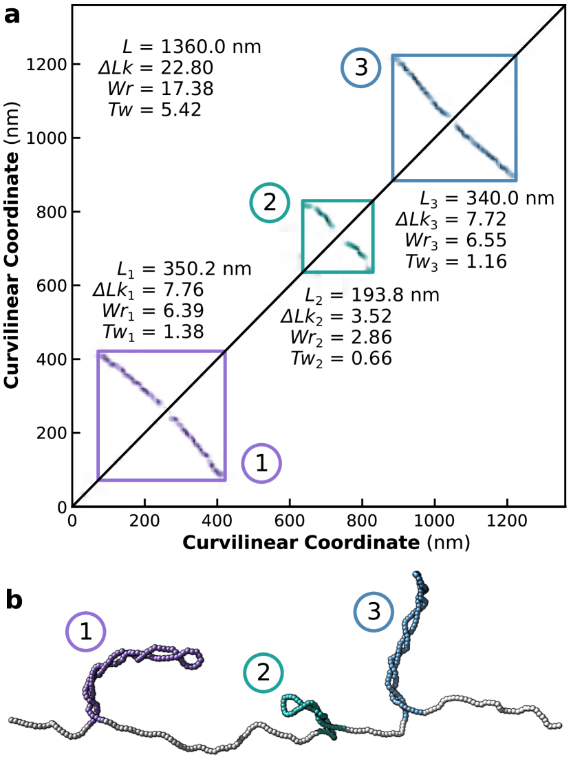
Figure 8: Illustration of the algorithm used to identify plectonemes in Monte Carlo generated snapshots. (a) Writhe map corresponding to the configuration shown in (b). The three plectonemes of panel (b) are highlighted by rectangles with corners $(i,i)$, $(i,j)$, $(j,i)$ and $(j,j)$ for a plectoneme with entry and exit indices $i$ and $j$, respectively. In the figure these indices have been converted into curvilinear coordinates. Writhe and twist can be calculated separately for each plectoneme, which allows for the calculation of the plectoneme linking number.

Here we outline the algorithm used to detect plectonemic regions in simulation generated configurations. Two different characteristics have been used in the past to identify plectonemes. For one, plectonemic coiling induces juxtaposition between sites that are far away along the DNA contour. Therefore, various studies, utilized a distance map (or contact map) to identify regions of high segment proximity [20, 43, 44]. Alternatively, one can identify plectonemes as regions of high writhe density [9, 42]. Writhe (defined below) is a measure of the amount of coiling of a closed curve [45], and plectonemes are characterized by a considerably larger writhe density as compared to the stretched phase (see Fig. 6 and [42, 46]).

In this work, we used the latter property to identify plectonemes. Since our simulations are composed of a series of $N-1$ straight segments $\mathbf{s}_{i}$ connecting consecutive beads, the double integral definition of writhe [45] may be decomposed into $(N-1)^{2}$ pairwise contributions 

$$\textrm{Wr}=\frac{1}{4\pi}\sum_{i=1}^{N}\sum_{j=1}^{N}\int_{\mathbf{s}_{i}}\int_{\mathbf{s}_{j}}\frac{\left(d\mathbf{r}_{j}\times d\mathbf{r}_{i}\right)\cdot\mathbf{r}_{ij}}{r_{ij}^{3}}=\sum_{i=1}^{N}\sum_{j=1}^{N}w_{ij}.$$ (55)

The elements $w_{ij}$ may then be viewed as analogous to the entries of a contact map. In practice, we calculate those elements $w_{ij}$ by analytically carrying out the double integral over the two straight segments $\mathbf{s}_{i}$ and $\mathbf{s}_{j}$ of length $a$ ($3.4$ nm in our case). For details on this calculation see method $1b$ from Ref. [48]. Note, that in the writhe map, plectonemes have much more contrast as compared to the proximity map  [42]. An example of a writhe map for a Monte Carlo generated configuration of length $L=1360$ nm ($4000$ bp or $400$ segments) containing 3 plectonemes is shown in Fig. 8. The high contrast black bands trace segment pairs $(s_{i},s_{j})$, where the $i$-th and $j$-the segment are on opposing strands along the superhelix. Towards the diagonal, as $i$ comes close to $j$, the trace approaches the plectoneme end-loop. Conversely, the outermost segments, indicated by the upper-left and lower-right corner of the rectangles drawn around the plectonemic region, mark the entry points of the plectonemes.

We trace plectonemes by setting a force dependent cutoff writhe-density $\chi_{\mathrm{min}}$, which is typically chosen, somewhere in-between the expected stretched and plectonemic phase supercoiling densities $\sigma_{s}$ and $\sigma_{p}$. Such choice can be made more quantitative by also considering the twist-density in the chain, which can either be directly calculated from the given snapshots or from the stretched phase theory [32, 49, 29]

$$\sigma_{Tw}=\left(1-\frac{C}{4A}\sqrt{\frac{k_{B}T}{Af}}\right)\sigma,$$ (56)

as twist is equilibrated over both phases. We then identify all indices $i$ for which the total involved writhe density is at least $\chi_{\mathrm{min}}$, i.e.

$$W_{i}\equiv\sum_{j=1}^{N-1}w_{i,j}>=\frac{a\omega_{0}}{2\pi}\chi_{\mathrm{min}}.$$ (57)

Neighbors among these remaining segments, say at indices $k$ and $l$ are then connected, if the sum of the intermediate contributions of $W_{i}$, including those at $k$ and $l$, still exceeds the minimum writhe density, i.e. if

$$\frac{1}{l-k+1}\sum_{j=k}^{l}W_{j}>=\frac{a\omega_{0}}{2\pi}\chi_{\mathrm{min}}.$$ (58)

This generates connected regions tracing one strand along a superhelical branch. The branch itself, can be traced by identifying for every $i$ the index $j$ for which the writhe contribution $|w_{ij}|$ is largest. Full plectoneme branches are finally identified by finding the pairs of strands which map into each other by inverting the respective indices, which is equivalent to transposing the points relative to the writhe map. Certain care has to be taken when tracing the branches, not to pick up contributions stemming from outside the current branch, which could in some cases lead to an erroneous assignment of a part of a stretched domain to a plectoneme. An exhaustive discussion of the algorithm is beyond the scope of this work. The final traces found for each plectoneme are indicated as colored lines in Fig. 8.

Once the plectonemic domains are identified the contained writhe can be extracted from the writhe map. The twist can either be taken directly from the simulation, if local twist strains are consisted, or in the case of equilibrated twist simulations [8, 50, 17] from the total twist $Tw=\Delta Lk-Wr$ of the entire snapshot. Summation of writhe and twist contained in the plectonemic domains yields the total linking number in the plectonemic phase, which together with the number of segments in in these domains yields the supercoiling density $\psi$. Completely analogously is the calculation of the the stretched phase supercoiling density $\phi$. Finally, the fraction of segments not contained in plectonemic domains gives the fractional occupancy of the stretched phase $\nu$.

References

- Vanderlinden et al. [2019] W. Vanderlinden, T. Brouns, P. U. Walker, P. J. Kolbeck, L. F. Milles, W. Ott, P. C. Nickels, Z. Debyser, and J. Lipfert, The free energy landscape of retroviral integration, Nature Comm. 10, 1 (2019).
- Yan et al. [2018a] Y. Yan, Y. Ding, F. Leng, D. Dunlap, and L. Finzi, Protein-mediated loops in supercoiled DNA create large topological domains, Nucl. Acids Res. 46, 4417 (2018a).
- Yan et al. [2018b] Y. Yan, F. Leng, L. Finzi, and D. Dunlap, Protein-mediated looping of DNA under tension requires supercoiling, Nucl. Acids Res. 46, 2370 (2018b).
- Yan et al. [2021] Y. Yan, W. Xu, S. Kumar, A. Zhang, F. Leng, D. Dunlap, and L. Finzi, Negative DNA supercoiling makes protein-mediated looping deterministic and ergodic within the bacterial doubling time, Nucl. Acids Res. 49, 11550 (2021).
- Marko and Siggia [1995a] J. F. Marko and E. D. Siggia, Statistical mechanics of supercoiled DNA, Phys. Rev. E 52, 2912 (1995a).
- Marko [2007] J. F. Marko, Torque and dynamics of linking number relaxation in stretched supercoiled DNA, Phys. Rev. E 76, 021926 (2007).
- Vologodskii et al. [1979] A. V. Vologodskii, V. V. Anshelevich, A. V. Lukashin, and M. D. Frank-Kamenetskii, Statistical mechanics of supercoils and the torsional stiffness of the DNA double helix, Nature 280, 294 (1979).
- Klenin et al. [1991] K. V. Klenin, A. V. Vologodskii, V. V. Anshelevich, A. M. Dykhne, and M. D. Frank-Kamenetskii, Computer Simulation of DNA Supercoiling, J. Mol. Biol. 217, 413 (1991).
- Vologodskii et al. [1992] A. V. Vologodskii, S. D. Levene, K. V. Klenin, M. Frank-Kamenetskii, and N. R. Cozzarelli, Conformational and thermodynamic properties of supercoiled DNA, J. Mol. Biol. 227, 1224 (1992).
- Marko and Siggia [1994] J. F. Marko and E. D. Siggia, Bending and twisting elasticity of DNA, Macromolecules 27, 981 (1994).
- Strick et al. [1996] T. R. Strick, J. F. Allemand, D. Bensimon, A. Bensimon, and V. Croquette, The elasticity of a single supercoiled DNA molecule, Science 271, 1835 (1996).
- Forth et al. [2008] S. Forth, C. Deufel, M. Y. Sheinin, B. Daniels, J. P. Sethna, and M. D. Wang, Abrupt buckling transition observed during the plectoneme formation of individual dna molecules, Phys. Rev. Lett. 100, 148301 (2008).
- Wada and Netz [2009] H. Wada and R. R. Netz, Plectoneme creation reduces the rotational friction of a polymer, EPL (Europhys. Lett.) 87, 38001 (2009).
- Neukirch and Marko [2011] S. Neukirch and J. F. Marko, Analytical description of extension, torque, and supercoiling radius of a stretched twisted DNA, Phys. Rev. Lett. 106, 138104 (2011).
- van Loenhout et al. [2012] M. van Loenhout, M. de Grunt, and C. Dekker, Dynamics of DNA supercoils, Science 338, 94 (2012).
- Oberstrass et al. [2012] F. C. Oberstrass, L. E. Fernandes, and Z. Bryant, Torque measurements reveal sequence-specific cooperative transitions in supercoiled DNA, Proc. Natl. Acad. Sci. USA 109, 6106 (2012).
- Lepage et al. [2015] T. Lepage, F. Képès, and I. Junier, Thermodynamics of Long Supercoiled Molecules: Insights from Highly Efficient Monte Carlo Simulations, Biophys. J. 109, 135 (2015).
- Fathizadeh et al. [2015] A. Fathizadeh, H. Schiessel, and M. R. Ejtehadi, Molecular dynamics simulation of supercoiled DNA rings, Macromolecules 48, 164 (2015).
- Benedetti et al. [2015] F. Benedetti, A. Japaridze, J. Dorier, D. Racko, R. Kwapich, Y. Burnier, G. Dietler, and A. Stasiak, Effects of physiological self-crowding of DNA on shape and biological properties of DNA molecules with various levels of supercoiling, Nucl. Acids Res. 43, 2390 (2015).
- Matek et al. [2015] C. Matek, T. E. Ouldridge, J. P. K. Doye, and A. A. Louis, Plectoneme tip bubbles: coupled denaturation and writhing in supercoiled DNA, Sci. Rep. 5, 7655 (2015).
- Ivenso and Lillian [2016] I. D. Ivenso and T. D. Lillian, Simulation of DNA supercoil relaxation, Biophys. J. 110, 2176 (2016).
- Barde et al. [2018] C. Barde, N. Destainville, and M. Manghi, Energy required to pinch a DNA plectoneme, Phys. Rev. E 97, 032412 (2018).
- Fosado et al. [2021] Y. A. Fosado, D. Michieletto, C. A. Brackley, and D. Marenduzzo, Nonequilibrium dynamics and action at a distance in transcriptionally driven DNA supercoiling, Proc. Natl. Acad. Sci. USA 118, e1905215118 (2021).
- Ott et al. [2020] K. Ott, L. Martini, J. Lipfert, and U. Gerland, Dynamics of the Buckling Transition in Double-Stranded DNA and RNA, Biophys. J. 118, 1690 (2020).
- De Vlaminck and Dekker [2012] I. De Vlaminck and C. Dekker, Recent advances in magnetic tweezers, Annu. Rev. Biophys. 41, 453 (2012).
- Lipfert et al. [2011] J. Lipfert, M. Wiggin, J. W. J. Kerssemakers, F. Pedaci, and N. H. Dekker, Freely orbiting magnetic tweezers to directly monitor changes in the twist of nucleic acids, Nature Comm. 2, 439 (2011).
- Vanderlinden et al. [2021] W. Vanderlinden, E. Skoruppa, P. Kolbeck, E. Carlon, and J. Lipfert, DNA fluctuations reveal the size and dynamics of topological domains, BiorXiv preprint https://doi.org/10.1101/2021.12.21.473646 (2021).
- Marko and Neukirch [2012] J. F. Marko and S. Neukirch, Competition between curls and plectonemes near the buckling transition of stretched supercoiled DNA, Phys. Rev. E 85, 011908 (2012).
- Emanuel et al. [2013] M. Emanuel, G. Lanzani, and H. Schiessel, Multiplectoneme phase of double-stranded DNA under torsion, Phys. Rev. E 88, 022706 (2013).
- Moroz and Nelson [1997] J. D. Moroz and P. Nelson, Torsional directed walks, entropic elasticity, and DNA twist stiffness, Proc. Natl. Acad. Sci. USA 94, 14418 (1997).
- Marko and Siggia [1995b] J. F. Marko and E. D. Siggia, Stretching DNA, Macromolecules 28, 8759 (1995b).
- Moroz and Nelson [1998] J. D. Moroz and P. Nelson, Entropic elasticity of twist-storing polymers, Macromolecules 31, 6333 (1998).
- Skoruppa et al. [2017] E. Skoruppa, M. Laleman, S. K. Nomidis, and E. Carlon, DNA elasticity from coarse-grained simulations: The effect of groove asymmetry, J. Chem. Phys. 146, 214902 (2017).
- Skoruppa et al. [2018] E. Skoruppa, S. K. Nomidis, J. F. Marko, and E. Carlon, Bend-Induced Twist Waves and the Structure of Nucleosomal DNA, Phys. Rev. Lett. 121, 088101 (2018).
- Skoruppa et al. [2021] E. Skoruppa, A. Voorspoels, J. Vreede, and E. Carlon, Length-scale-dependent elasticity in DNA from coarse-grained and all-atom models, Phys. Rev. E 103, 042408 (2021).
- Bouchiat and Mézard [1998] C. Bouchiat and M. Mézard, Elasticity model of a supercoiled DNA molecule, Phys. Rev. Lett. 80, 1556 (1998).
- Bouchiat and Mézard [2000] C. Bouchiat and M. Mézard, Elastic rod model of a supercoiled DNA molecule, Eur. Phys. J. E 2, 377 (2000).
- Gao et al. [2021] X. Gao, Y. Hong, F. Ye, J. T. Inman, and M. D. Wang, Torsional stiffness of extended and plectonemic dna, Phys. Rev. Lett. 127, 028101 (2021).
- Rybenkov et al. [1993] V. V. Rybenkov, N. R. Cozzarelli, and A. V. Vologodskii, Probability of DNA knotting and the effective diameter of the DNA double helix, Proc. Natl. Acad. Sci. USA 90, 5307 (1993).
- Frenkel and Smit [2002] D. Frenkel and B. Smit, Understanding Molecular Simulation: From Algorithms to Applications, 2nd ed., Computational Science Series, Vol. 1 (Academic Press, San Diego, 2002).
- Kumar et al. [1992] S. Kumar, J. M. Rosenberg, D. Bouzida, R. H. Swendsen, and P. A. Kollman, The weighted histogram analysis method for free-energy calculations on biomolecules. i. the method, J. Comp. Chem. 13, 1011 (1992).
- Liu and Chan [2008] Z. Liu and H. S. Chan, Efficient chain moves for Monte Carlo simulations of a wormlike DNA model: Excluded volume, supercoils, site juxtapositions, knots, and comparisons with random-flight and lattice models, J. Chem. Phys. 128, 145104 (2008).
- Coronel et al. [2018] L. Coronel, A. Suma, and C. Micheletti, Dynamics of supercoiled DNA with complex knots: large-scale rearrangements and persistent multi-strand interlocking, Nucl. Acids Res. 46, 7533 (2018).
- Desai et al. [2020] P. R. Desai, S. Brahmachari, J. F. Marko, S. Das, and K. C. Neuman, Coarse-grained modelling of DNA plectoneme pinning in the presence of base-pair mismatches, Nucl. Acids Res. 48, 10713 (2020).
- Fuller [1971] F. B. Fuller, The Writhing Number of a Space Curve, Proc. Natl. Acad. Sci. USA 68, 815 (1971).
- Marko [2015] J. F. Marko, Biophysics of protein-DNA interactions and chromosome organization, Physica A 418, 126 (2015).
- Note [1] We remark that writhe is technically only defined for a closed space curve, which in the context of stretched linear DNA is usually resolved by introducing a virtual closure at either infinity or through a large arc [51, 52]. We ignore these closure contributions, since they are irrelevant for the detection of plectonemes.
- Klenin and Langowski [2000] K. Klenin and J. Langowski, Computation of writhe in modeling of supercoiled DNA, Biopolymers 54, 307 (2000).
- Nomidis [2020] S. K. Nomidis, Theory and simulation of DNA mechanics and hybridization, Ph.D. thesis, KU Leuven (2020).
- Yang et al. [2000] Z. Yang, Z. Haijun, and O. Y. Zhong-Can, Monte Carlo implementation of supercoiled double-stranded DNA, Biophys. J. 78, 1979 (2000).
- Vologodskii and Marko [1997] A. V. Vologodskii and J. F. Marko, Extension of torsionally stressed DNA by external force, Biophys. J. 73, 123 (1997).
- Chou et al. [2014] F. C. Chou, J. Lipfert, and R. Das, Blind predictions of DNA and RNA tweezers experiments with force and torque, PLoS Comp. Biol. 10, e1003756 (2014).