Exploring Diversity-based Active Learning for 3D Object Detection in Autonomous Driving

Abstract

3D object detection has recently received much attention due to its great potential in autonomous vehicle (AV). The success of deep learning based object detectors relies on the availability of large-scale annotated datasets, which is time-consuming and expensive to compile, especially for 3D bounding box annotation. In this work, we investigate diversity-based active learning (AL) as a potential solution to alleviate the annotation burden. Given limited annotation budget, only the most informative frames and objects are automatically selected for human to annotate. Technically, we take the advantage of the multimodal information provided in an AV dataset, and propose a novel acquisition function that enforces spatial and temporal diversity in the selected samples. We benchmark the proposed method against other AL strategies under realistic annotation cost measurement, where the realistic costs for annotating a frame and a 3D bounding box are both taken into consideration. We demonstrate the effectiveness of the proposed method on the nuScenes dataset and show that it outperforms existing AL strategies significantly.

I Introduction

3D object detection has recently received much attention from the 3D computer vision community due to its great potential in autonomous vehicle (AV). Most works are focused on improving the detection accuracy by designing more effective network architectures [1, 2, 3] and input representations [4, 5, 6, 7]. The success of these deep learning based methods relies on the availability of large-scale annotated datasets, the collection of which is time consuming and prohibitively expensive; this is particularly true for 3D bounding box annotation in point cloud data, where the annotator needs to adjust the yaw angle frequently for accurate labeling. This necessitates the development of data-efficient learning techniques for 3D object detection to reduce the labeling efforts.

Active learning (AL) offers a promising solution to mitigate the annotation burden. Given a limited annotation budget, AL aims to maximize model performance by iteratively selecting the most informative samples to label based on current model state. Depending on how the informativeness is measured, various methods can be generally categorized into uncertainty-based [8, 9, 10], diversity-based [11, 12] and hybrid methods [13, 14, 15]. Due to the data-hungry nature of deep learning, there is a resurgence of interest of AL in recent years. It has been shown to achieve comparable accuracy with relatively fewer labels for image classification [16, 17, 18], 2D object detection [19, 20, 21] and semantic segmentation [22, 23, 24].

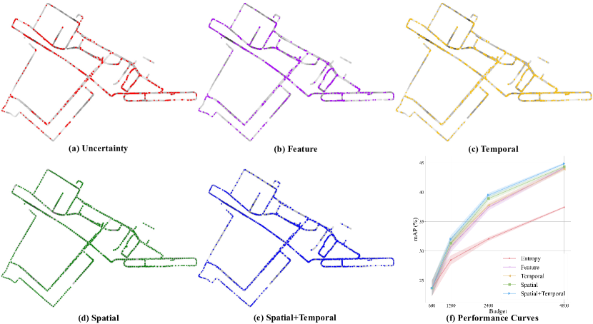
Figure 1: Distribution of samples selected by different active learning strategies and the corresponding performance - (a) Uncertainty, (b) Feature Diversity, (c) Temporal Diversity, (d) Spatial Diversity and (e) Combined Spatial and Temporal Diversity. (f) Performance curves on nuScenes. Colors represent different selection strategies. The black-white color scale along the path represents original data distribution density (black indicates high density). The proposed spatial and temporal diversity is able to select a diverse of samples without the need of a good feature extractor, while uncertainty-based sampling tends to concentrate in regions of high data density, resulting in redundant samples being selected.

Little attention has been paid to AL for 3D object detection, and Feng et al.[25] made the first attempt by employing uncertainty-based sampling to query unlabeled samples. However, the method developed in [25] is entangled with frustum-based detectors, and a general AL method that can be universally applied to all existing detectors is lacking. Also, diversity-based AL is not studied in [25], and it is not clear whether and how the multimodal information that is typically available in an AV dataset can be utilized for querying informative samples. Our work fills this gap.

In this work, we focus on diversity-based AL for 3D object detection and propose that enforcing diversity in the spatial and temporal space achieves superior performance. Our method is motivated by the observation that data collected by the autonomous vehicle at different locations and time steps corresponds to different scenes and visual content, and by enforcing diversity in the location and time steps of the selected samples, we can obtain a diverse set of samples covering different object categories. Figure 1 summarizes the behavior of different AL strategies and the corresponding performance curves. The proposed spatial and temporal diversity can effectively select a diverse set of informative samples and achieve the best detector performance at the same budget.

An important consideration in applying AL for 3D object detection is how to measure the annotation cost. Previous works measure the annotation cost either by the number of annotated frames [21, 19, 26] or the number of annotated bounding boxes [27, 28]. The former is inaccurate as different frames contain different number of objects and the actual annotation cost can differ significantly. The latter ignores the fact that even an almost empty frame takes time for the annotator to look for objects of interest. We thus consider a more realistic setting where both the cost for annotating a frame and a 3D bounding box are taken into consideration.

Finally, we look into the cold-start problem of AL, i.elet@tokeneonedot, the first batch of samples are usually randomly selected (as a trained model is not available for active selection of the initial batch) [28] and results in sub-optimal solution. We show that the proposed acquisition function can effectively provides a warm-start for the AL cycles.

Our contributions can be summarized as below:

• We propose a novel diversity-based acquisition function for AL in 3D object detection. We exploit the multimodal information provided in an AV dataset and propose spatial and temporal diversity objectives for querying informative samples.

• We propose to evaluate the AL methods under realistic annotation cost measurement. We show that the choice of cost measurement can significantly affect the evaluation results and highlight the importance of using realistic cost measurement to properly evaluate AL methods.

• We look into the cold-start problem of AL and demonstrate that the proposed acquisition function can provide an effective solution to this.

II Related Work

II-A Active Learning for Deep CNNs

The success of deep CNNs on visual recognition tasks relies on the availability of large-scale annotated datasets. Active learning offers a promising solution to alleviate annotation efforts and there is a resurgence of interest in AL in the deep learning era [29]. Acquisition function is the core component in AL, and various AL strategies can be generally categorized into uncertainty-based and diversity-based methods. Uncertainty-based AL [8, 9, 30, 13, 10] select the most uncertainty samples to label and different methods vary in how the uncertainty is estimated. [31] obtained the uncertainty through the estimation of an ensemble of classifiers. Learning-Loss[10] proposed to use the pseudo loss as an indication of uncertainty. Diversity-based AL [11, 32, 12, 33, 34] select the most diverse set of samples to label. Core-Set [11] formulated the AL problem as minimizing the core-set loss and proposed solutions to minize the upper-bound of the core-set loss. VAAL [34] trained an auto-encoder in an adversarial manner and select unlabeled samples that are most dissimilar with labeled ones based on the discriminator score. Our method is based on the Core-Set framework, and we propose novel diversity objectives to complement the traditionally used feature diversity.

II-B Active Learning for Object Detection

Several attempts have been made to apply AL for object detection tasks, and most of them are focused on 2D object detection task. Aghdam et al. [19] proposed to obtain an image-level score by aggregating pixel-wise scores for active selection. Instead of aggregating pixel-wise scores, Brust et al. [35] investigate various methods to aggregate bounding box scores. Roy et al. [20] utilized the disagreement of layer-wise prediction scores for query and the method is specific to one-stage object detectors with similar architecture of SSD [36]. Kao et al. [21] combined the uncertainty in both classification and location prediction to query samples. These AL methods are specifically optimized for 2D object detection and are entangled with the architecture of 2D object detectors, and thus a direct application to 3D object detection is either infeasible or sub-optimal. The only work we are aware that tackles AL for 3D object detection is reported in [25], but the method is entangled with frustum-based detectors and only uncertainty-based AL is investigated. In this work, we focus on diversity-based AL and our method is agnostic to the detector architecture.

II-C 3D Object Detection

Depending on how the point cloud data is represented, existing 3D object detectors can be divided into two categories : point-based and voxel-based methods. Point-based detectors[37, 1, 38, 4, 39] use the point-wise feature extractor[40, 41, 42] as backbone and directly extract point-wise feature from the input point cloud. Proposals are generated based on the position of point cloud, which can provide more fine-grained position information. However, point-based methods typically downsample the input point cloud to a fixed number of points, and some input information may be lost. Voxel-based detectors[43, 7, 2, 3, 44, 45] quantize the input point cloud as regular voxels, and utilize 3D CNNs to operate on voxels directly. The extracted 3D feature map are then projected into a bird-eye-view(BEV) feature map and proposals are generated from the projected 2D feature map. While voxelization can cause the loss of fine-grained position information, it has the advantage of establishing regularities for the irregular point cloud, and allowing for the use of powerful 3D CNNs to extract features. We employ one of the state-of-the-art voxel-based detectors, VoxelNet [43], as detection model to perform experiments, but our method is compatible with all existing detectors.

III Methodology

The overview of the proposed AL pipeline for 3D object detection is presented in Fig. 2. AL is an iterative process where in each cycle, an informative subset of samples are selected based on an acquisition function. The selected samples are then sent to an oracle for annotation and the model is updated on all the samples annotated so far. The process is iterated until the annotation budget is exhausted. In the following, we will first introduce the diversity-based AL framework. We then describe in details our proposed acquisition function that incorporates novel spatial and temporal diversity objectives. Finally, we present a realistic method to measure annotation cost.

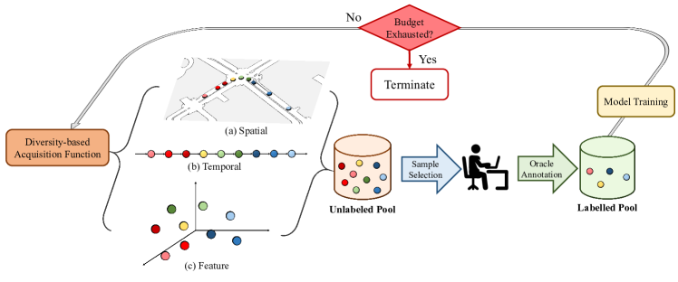
Figure 2: The proposed AL pipeline for 3D object detection. The spatial, temporal and feature diversity terms are complementary to each other.

III-A Diversity-based AL

Diversity-based AL selects to label a diverse subset of samples that can represent the distribution of the unlabeled pool. Core-Set [11] is one of the state-of-the-art methods for diversity-based AL. It formulates the AL problem as minimizing the core-set loss, i.elet@tokeneonedot, selecting a set of points such that the difference between the average empirical training loss on this subset and the average empirical loss on the entire dataset is minimized. [11] showed that minimizing the upper bound of the core-set loss is equivalent to solving a k-Center problem. Mathematically, denoting the unlabeled pool as $\mathcal{S}_{u}=\{\mathbf{x}_{i}\}_{i=1\cdots N_{u}}$ and the labeled pool as $\mathcal{S}_{l}=\{\mathbf{x}_{j}\}_{j=1\cdots N_{l}}$, at each AL cycle $t$, we are trying to select a subset $\mathcal{B}_{t}$ from $\mathcal{S}_{u}$ by solving the k-Center objective:

$$\min_{\mathcal{B}_{t}\subseteq\mathcal{S}_{u}}\max_{\mathbf{x}_{i}\in\mathcal{B}_{t}}\min_{\mathbf{x}_{j}\in\mathcal{B}_{t}\cup\mathcal{S}_{l}}d(\mathbf{x}_{i},\mathbf{x}_{j}),\quad s.t.\quad\mathcal{C}(\mathcal{B}_{t})\leq b_{t},$$ (1)

where $d(\cdot,\cdot)$ is a distance measure between two samples, $\mathcal{C}(\cdot)$ is the annotation cost for labeling a subset, and $b_{t}$ is the annotation budget for cycle $t$. Solving Eq. (1) is NP-hard, and we opt for a greedy solution for AL selection, which is summarized in Algorithm 1.

Algorithm 1 Greedy solution for AL selection

1:Budgets $\{b_{0},\ b_{1},\ \ldots,\ b_{T-1}\}$; Dataset $\mathcal{S}$

2:Initialize the label set $\mathcal{S}_{l}$ with $\mathcal{C}(\mathcal{S}_{l})\leq b_{0}$

3:Initialize the unlabeled set $\mathcal{S}_{u}=\mathcal{S}\setminus\mathcal{S}_{l}$

4:for $t=1,\ \ldots,T-1$ do

5:     $\mathcal{B}_{t}=\emptyset$ 

6:     $\tilde{b}$ = 0

7:     while $\tilde{b}<b_{t}$ do

8:         $\tilde{\mathbf{x}}=\arg\max_{\mathbf{x}_{i}\in\mathcal{S}_{u}}\min_{\mathbf{x}_{j}\in\mathcal{S}_{l}\cup\mathcal{B}_{t}}d(\mathbf{x}_{i},\mathbf{x}_{j})$

9:         $\mathcal{B}_{t}\leftarrow\mathcal{B}_{t}\cup\tilde{\mathbf{x}}$

10:         $\mathcal{S}_{u}\leftarrow\mathcal{S}_{u}\setminus\tilde{\mathbf{x}}$

11:         $\tilde{b}\leftarrow\mathcal{C}(\mathcal{B}_{t})$

12:     end while

13:     Annotate the samples in $\mathcal{B}_{t}$

14:     $\mathcal{S}_{l}\leftarrow\mathcal{S}_{l}\cup\mathcal{B}_{t}$

15:     Train detector $\Phi_{t}$ on $\mathcal{S}_{l}$

16:end for

17:return Detector $\Phi_{T-1}$;

A common practice to measure $d(\mathbf{x}_{i},\mathbf{x}_{j})$ is to embed the samples in a feature space using a feature extractor $\Theta$ and compute the distance by $L_{p}$ norm:

$$d_{f}(\mathbf{x}_{i},\mathbf{x}_{j})=||\Theta(\mathbf{x}_{i})-\Theta(\mathbf{x}_{j})||_{p}.$$ (2)

However, it is non-trivial to design a good feature extractor for the task. In the following section, we explore how the multimodal information in an AV dataset can be utilized to design more effective diversity terms.

III-B Enforcing Diversity in Spatial and Temporal Space

Existing AV datasets comprise multimodal data including images, point clouds and GPS/IMU data. The multimodal data is complementary to each other and how to combine multimodal measurements in a principled manner for robust detection has attracted much attention from the AV community. While most works focus on fusing image and point cloud data for 3D object detection[46, 47], we are interested in exploiting the GPS/IMU data for active learning of 3D object detectors.

The GPS/IMU system provides accurate location information for the vehicle. Intuitively, different location traversed by the autonomous vehicle corresponds to different scenes and visual content, and by enforcing diversity in the location of the selected samples, we can obtain a diverse set of samples covering different object categories without relying on a good feature extractor. This motivates us to design a spatial diversity objective for the k-Center optimization. Furthermore, we observe that an autonomous driving vehicle may visit the same place at different timings for data collection, and the data collected at the same location but different timings vary in traffic and weather conditions. We thus propose to enforce diversity in temporal space to complement the spatial diversity for optimal sample selection. We detail the definition of the proposed spatial and temporal diversity objectives in the following.

Spatial Diversity Objective As the multi-modal sensors are synchronized during data collection, each sample in $\mathcal{S}_{u}$ is associated with a spatial location. Denoting the location of sample $\mathbf{x}_{i}$ as $loc(\mathbf{x}_{i})$, we measure the spatial distance between two samples by manifold distance. Specifically, we first build a KNN graph with adjacency matrix $\mathbf{W}\in R^{(N_{l}+N_{u})\times(N_{l}+N_{u})}$ defined as below,

$$w_{ij}=\begin{cases}||loc(\mathbf{x}_{i})-loc(\mathbf{x}_{j})||_{2}^{2},&\text{if }\mathbf{x}_{i}\in NN_{k}(\mathbf{x}_{j})\\ 0.&\text{otherwise}\end{cases}$$ (3)

where $NN_{k}(\cdot)$ is the set of k-nearest neighbors for a sample in the Euclidean space. The spatial distance between $\mathbf{x}_{i}$ and $\mathbf{x}_{j}$ is then defined as their shortest path on the KNN graph. This problem can be efficiently solved by Dijkstra’s algorithm:

$$\begin{split}&d_{s}(\mathbf{x}_{i},\mathbf{x}_{j})=\min_{\{c_{pq}\}}\sum_{p,q=1,\cdots,(N_{l}+N_{u})}w_{pq}c_{pq}\\ &s.t.\quad c_{pq}\geq 0\text{ and }\forall p,\sum_{q}c_{pq}-\sum_{q}c_{qp}=\begin{cases}1,\text{if }p=i\\ -1,\text{if }p=j\\ 0.\text{otherwise}\end{cases}\end{split}$$ (4)

For samples collected from different areas, e.g. one sample collected from Singapore vs. another collected from Boston, we define the spatial distance as a large constant.

Temporal Diversity Objective A sample in an AV dataset is also associated with a data stream id $si\in N^{1}$ and the timestamp $ts\in R^{1}$. We define the temporal distance as below,

$$d_{t}(\mathbf{x}_{i},\mathbf{x}_{j})=\begin{cases}|ts(\mathbf{x}_{i})-ts(\mathbf{x}_{j})|,\ \text{if}\ si(\mathbf{x}_{i})=si(\mathbf{x}_{j})\\ \inf.\ \text{otherwise}\end{cases}$$ (5)

III-C Combining Diversity Terms

The various diversity terms, e.g. spatial, temporal and feature, defined above are complementary to each other and we can combine them to achieve better performance. As the values for each diversity objective are in different scales, we first normalize it to [0, 1] using a radial basis function (RBF) kernel. Specifically, for the spatial diversity term $d_{s}(\mathbf{x}_{i},\mathbf{x}_{j})$, we normalize it by the following equation:

$$\bar{d}_{s}(\mathbf{x}_{i},\mathbf{x}_{j})=1-\exp(-d_{s}(\mathbf{x}_{i},\mathbf{x}_{j})).$$ (6)

The temporal diversity term $d_{t}$ and $d_{f}$ can be similarly normalized. The distance metric used in Algorithm 1 is then defined as:

$$d(\mathbf{x}_{i},\mathbf{x}_{j})=\lambda_{s}\bar{d}_{s}(\mathbf{x}_{i},\mathbf{x}_{j})+\lambda_{t}\bar{d}_{t}(\mathbf{x}_{i},\mathbf{x}_{j})+\lambda_{f}\bar{d}_{f}(\mathbf{x}_{i},\mathbf{x}_{j}).$$ (7)

III-D Annotation Cost Measurement

In contrast to previous works that use either the number of annotated frames or the number of annotated bounding boxes to measure annotation cost, we propose to take into consideration the cost of annotating both. Specifically, the annotation cost $\mathcal{C}(\mathcal{B}_{t})$ used in Eq. (1) and Algorithm 1 is computed as:

$$\ \mathcal{C}(\mathcal{B}_{t})=c_{f}*n_{f}({\mathcal{B}_{t}})+c_{b}*n_{b}({\mathcal{B}_{t}}),$$ (8)

where $c_{f}$ and $c_{b}$ is the cost for annotating one frame and one bounding box, respectively, and $n_{f}$ and $n_{b}$ denote the total number of frames and bounding boxes in the selected samples. The actual value for $c_{f}$ and $c_{b}$ varies among different vendors. In the experiments, we set the values based on discussion with the nuScenes team and investigate the influence of different settings in Section V-C.

IV Experiment

IV-A Experimental Settings

Evaluation Datasets We perform experiments on the nuScenes[48], which is a popular multimodal dataset used for benchmarking 3D object detection algorithms. The training set of nuScenes contains 28,130 LiDAR point clouds and 1,255,109 bounding boxes, and the validation set of nuScenes contains 6,019 LiDAR point clouds. The nuScenes contains 10 categories, namely: car, truck, construction vehicle, bus, trailer, barrier, motorcycle, bicycle, pedestrian, traffic cone and ignore. We perform active selection on the training set and report the detector performance on the validation set.

Evaluation Metrics Following the official nuScenes evaluation protocol, we report mean Average Precision(mAP) as the evaluation metric to compare different methods.

Detection Model We employ the open-source VoxelNet[43] as our 3D object detection detector in all experiments. We voxelize the input point clouds in the range of $[-51.2,51.2]$, $[-51.2,51.2]$ and $[-5.0,3.0]$ for axis x, y, z, respectively.

Fully Supervised Baseline We train a detector using the entire training set, which serves as a performance upper bound for all AL methods. We follow the default training setting in VoxelNet[43]. For nuScenes, we trained for a total 20 epoches with a batch size of 8. The mAP of the fully supervised baseline is 51.00%.

Implementation Details We perform sample selection at the granularity of frame, and once a frame is selected, all the objects of interest within the frame are annotated. We set $c_{s}=0.12,\ c_{b}=0.04$ in Eq.  8. With this setting, the budget for annotating the entire training set in nuScenes is $36,314$. We conduct AL at the budget of 600/1200/2400/4800. The number of nearest neighbor used in constructing the KNN graph for computing spatial diversity is set to $K=8$. The training hyper-parameters remain the same as the fully supervised baseline. We conduct each experiment three-times and report the average result.

IV-B Experimental Results

Comparing Different Diversity Terms We consider three diversity terms, i.elet@tokeneonedot, feature, spatial and temporal, to measure the distance between two samples. We set the random selection as baseline and investigate the effect of each diversity term and their combination on AL performance. We consider the following variants:

(A) Random: This strategy randomly select the samples.

(B) Feature [11]: This strategy uses Eq. (2) to measure sample distance. We obtain the feature of each sample used in Eq. 2 by averaging the output feature map of the 3D feature extractor.

(C) Spatial [23]: This strategy uses Eq. (LABEL:EqDs) to measure sample distance.

(D) Temporal: This strategy uses Eq. (5) to measure sample distance.

(E) Spatial+Temporal: This strategy uses Eq. (7) with $\lambda_{s}=1,\lambda_{t}=1,\lambda_{f}=0$ to measure sample distance.

(F) Spatial+Temporal+Feature: This strategy uses Eq. (7) with $\lambda_{s}=1,\lambda_{t}=1,\lambda_{f}=1$ to measure sample distance.

For fair comparison, the first batch (budget=600) is randomly selected and kept the same for all methods. The results are presented in Table I. It can be seen that Spatial+Temporal outperforms the traditionally used Feature diversity, and perform comparably to Spatial+Temporal+Feature without the need of feature engineering.

Budget	Random	Feature [11]	Spatial [23]	Temporal	Spa+Temp	Spa+Temp+Feat
1200	30.23	30.71	31.33	31.20	31.22	31.22
2400	37.52	37.47	38.28	37.48	39.15	39.23
4800	42.61	44.15	43.68	43.30	44.37	44.77

TABLE I: Comparing different diversity terms. Spatial, Temporal and Features are shorten as Spa, Temp and Feat respectively for representing combination multi terms. Feature term in Spa+Temp+Feat is enabled at budget 1200.

Comparing with Uncertainty-based Sampling For AL, Uncertainty-based sampling has been widely used in various visual recognition tasks. It aims to select samples that the current model is most uncertain of. One drawback of uncertainty-based sampling comes from the observation that neural networks tends to predict similar output for similar input, and thus similar samples will have similar uncertainty values. Directly selecting the top-k uncertain samples will result in a set of redundant samples. This problem is more severe on AV datasets, where the velocity of the autonomous vehicle is affected by the traffic condition, resulting in different sampling density at different parts of the path, e.g. slower velocity results in higher sampling density as the recording rate of the sensors is fixed. Regions with high sampling density usually correspond to busy scenes that contain a relatively large number of objects. The object detector has relatively low confidence (high uncertainty) on these scenes, and thus will be picked up by uncertainty-based sampling. However, the high sampling density of these scenes will cause uncertainty-based sampling to select a set of uncertain yet redundant samples, which harm the training of the object detector. State-of-the-art uncertainty-based sampling methods typically adopt a “first randomly sample a large pool, then select the top-k uncertain ones" approach to alleviate this problem [10]. However, as showed in Fig. 3, uncertainty-based sampling still underperform the Random baseline on AV dataset, while the vanilla diversity-based AL method (i.elet@tokeneonedot, feature diversity) significantly outperforms the rest.

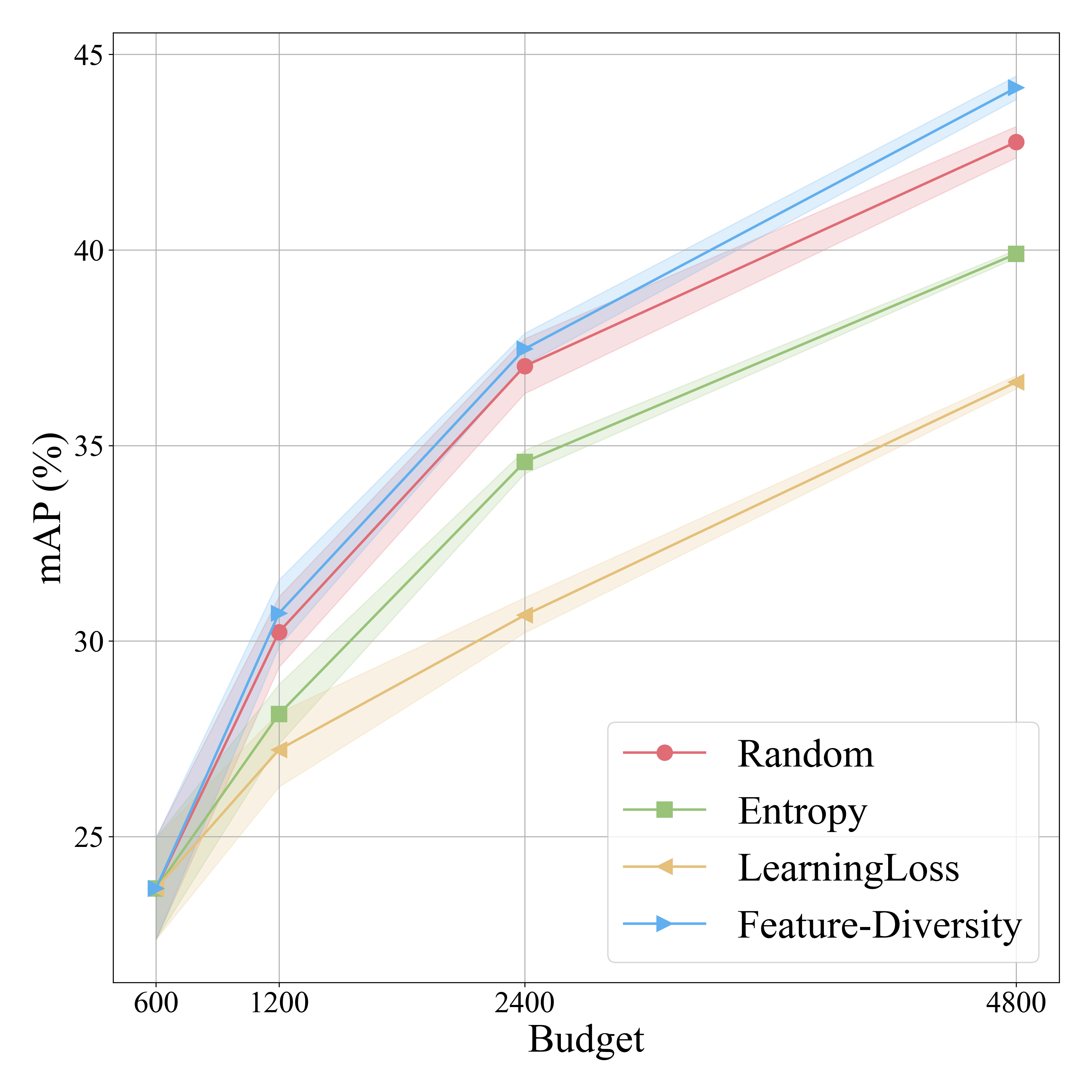
Figure 3: Comparing uncertainty-based sampling and diversity-based sampling for AL on nuScenes dataset.

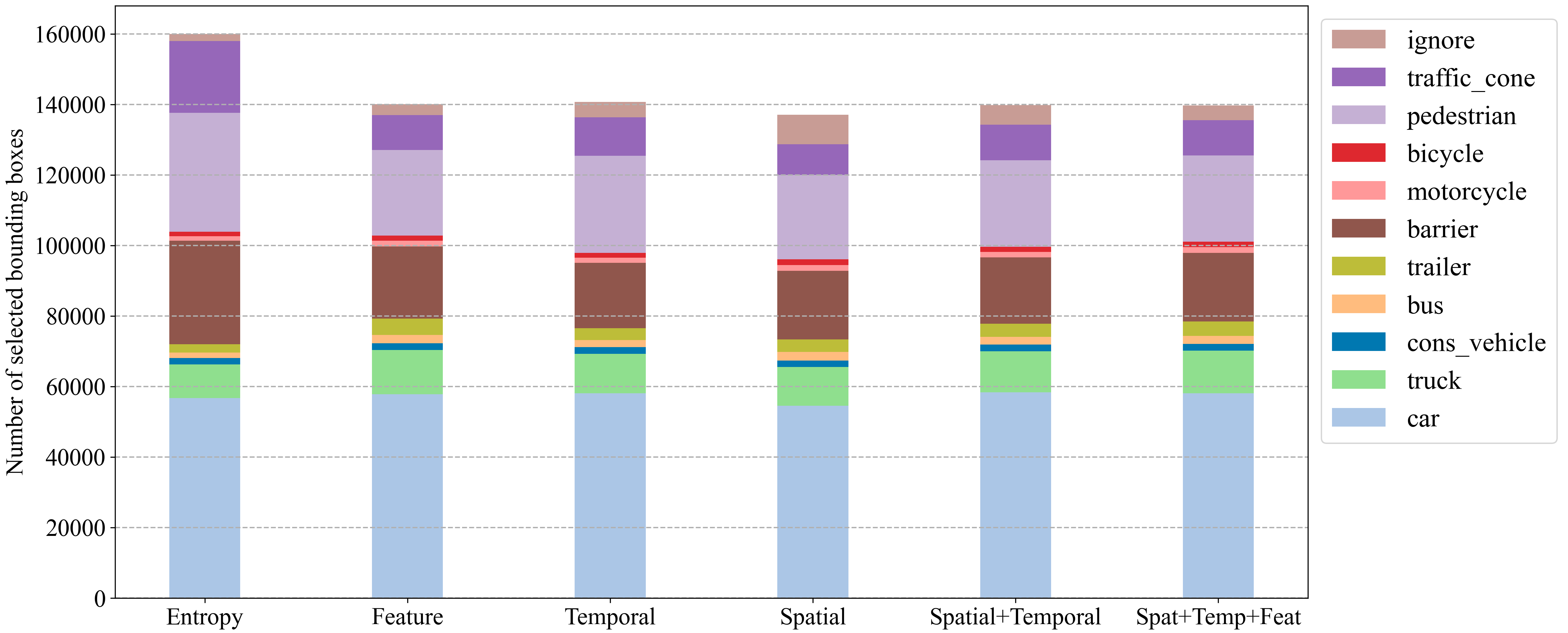
Figure 4: Distribution of selected bounding boxes over categories at budget 4800.

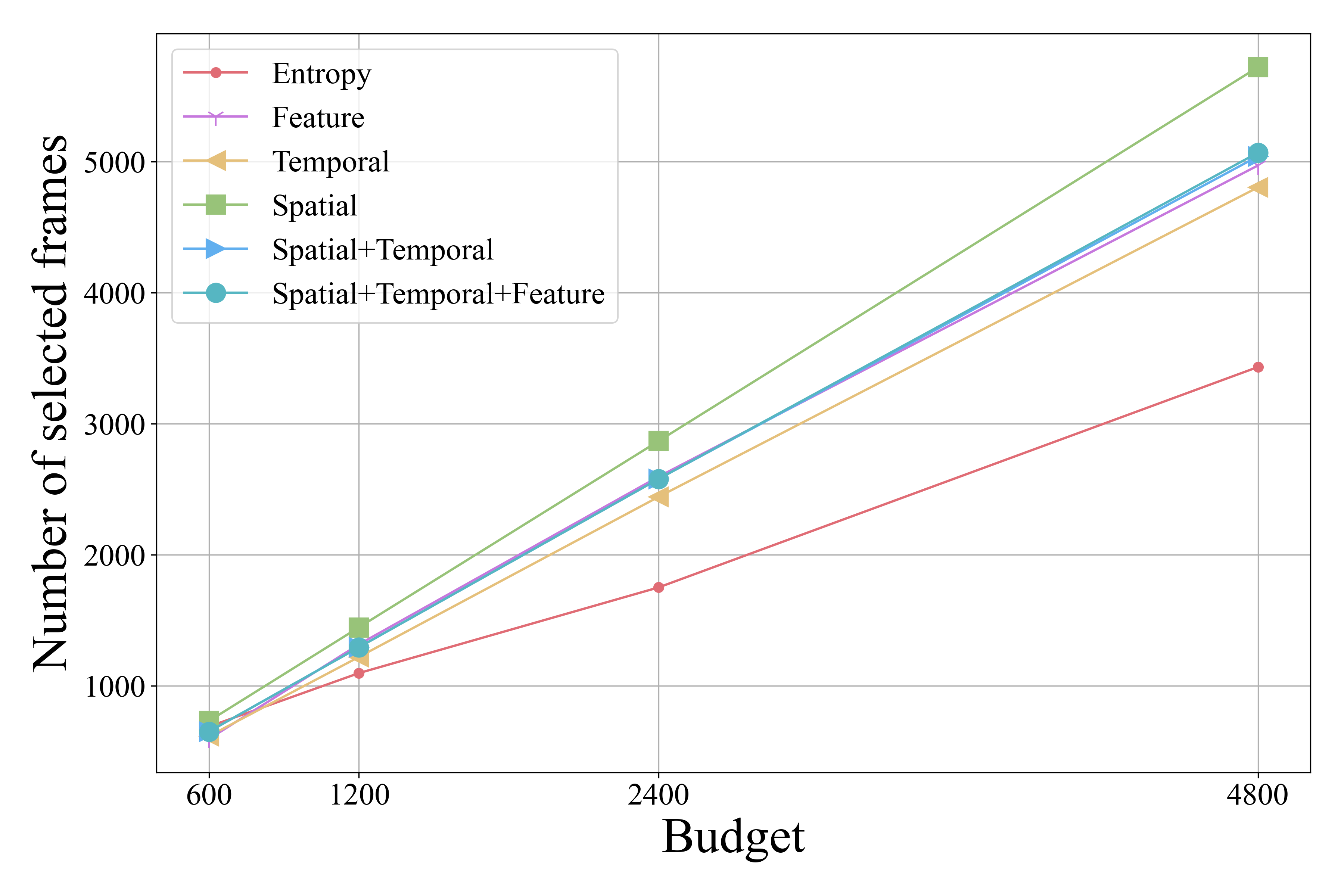
Figure 5: Number of frames selected by different strategies at fixed budgets.

V Discussion

V-A Selected Sample Distribution

To cast more insight into why diversity-based AL works better than uncertainty-based AL, we visualize the distribution of frames selected by different acquisition functions in Fig. 1, the category distribution of selected bounding boxes in Fig. 4, and the number of selected frames in Fig. 5. It can be seen that Entropy selects the most number of bounding boxes and the least number of frames. This suggests that Uncertainty tends to concentrate the annotation budget in regions with high sampling density, and these regions typically correspond to busy streets where the number of objects within each scene is high. On the contrary, Spatial selects the most number of frames and the least number of bounding boxes, and the selected frames are distributed uniformly over all regions. The distribution of samples selected by Feature and Temporal lie in the middle, and the diversity terms complement each other to select an informative subset of samples to label.

In detail, we visualize the distribution of samples selected by different selection strategies at one segment in Fig. 6. For each strategy, we randomly select 40 samples and visualize the corresponding images taken by the front camera. It can be seen that Uncertainty tends to select highly similar samples. Feature is able to select more diverse samples but there is still some redundancy. Spatial+Temporal can complement Feature and further improve the diversity of selected samples.

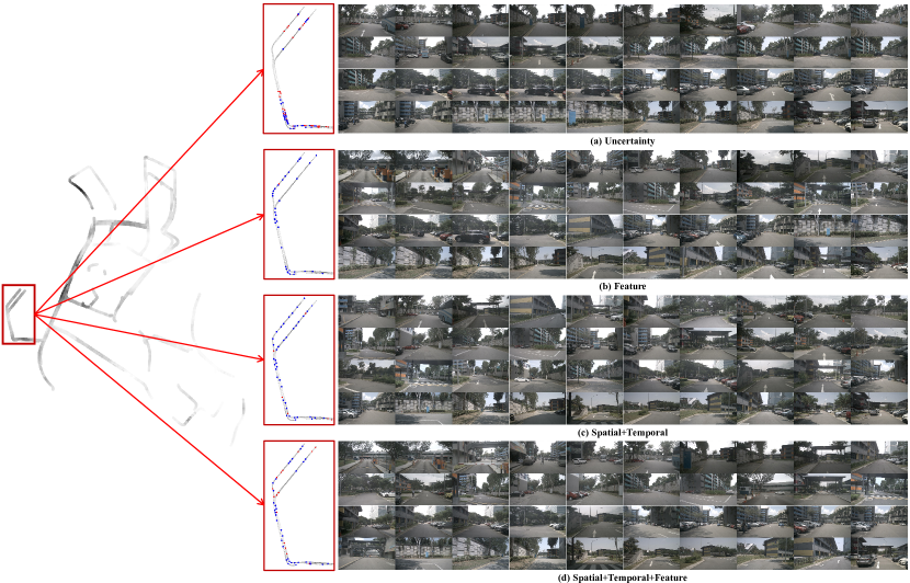
Figure 6: Visualization of samples selected by different acquisition functions. • indicates selected samples and • indicates those selected samples whose front camera view are visualized on the right.

V-B Initial Batch Selection

Typically, the AL acquisition function is contingent on the model prediction. For example, uncertainty-based AL depends on the model prediction score, and feature diversity-based AL utilizes the model for feature extraction. At the early stage of the AL cycles, due to data scarcity and model instability, AL strategies may fail. This is called the cold-start problem of AL [49]. One advantage of our proposed spatial and temporal diversity is that it does not rely on model prediction, and thus can be utilized to select betters samples for initializing the AL cycles.

In Section IV-B, we fix the initial batch (selected by Random) for all methods for fair comparison. In Table II, we provide additional results where the initial batch is selected by Spatial+Temporal. It can be seen that using the proposed method not only achieves higher accuracy at early batches, but also results in better performance in the long run.

	600	1200	2400	4800
Random	23.67	30.23	37.52	42.61
Spatial+Temporal(cold)	23.67	31.22	39.15	44.37
Spatial+Temporal(warm)	24.82	32.03	39.51	44.85
Spatial+Temporal+Feature(cold)	23.67	31.22	39.23	44.77
Spatial+Temporal+Feature(warm)	24.82	32.03	39.31	45.02

TABLE II: Comparing the effect of selecting the initial batch by Random (cold) or Spatial+Temporal (warm).

V-C Influence of Cost Measurement

We set the cost for annotating a frame ($c_{f}$) to 0.12, and the cost for annotating a 3D bounding box ($c_{b}$) to 0.04. These values reflect the market rates charged by big data annotation companies in US . The ratio $c_{f}/c_{b}$ can vary among companies and may affect the evaluation results. We experiment with extreme condition where the vendor only charges for bounding box annotation ($c_{f}=0,c_{b}=0.04$, equivalent to measuring annotation cost by the number of selected bounding boxes) or for frame annotation ($c_{f}=0.6,c_{b}=0$, equivalent to measuring annotation cost by the number of selected frames). The results are presented in Table III. It can be seen that how the cost is measured can significantly affect the relative ranking or the gap of different AL strategies. For example, when only frame annotation is charged, Random emerges as a strong baseline, and the gap between Entropy and other methods is greatly reduced. This highlights the importance of using realistic annotation cost measurement to properly evaluate different methods.

	600	1200	2400	600	1200	2400	600	1200	2400
	$c_{f}=0.12,c_{b}=0.04$			$c_{f}=0.0,c_{b}=0.04$			$c_{f}=0.6,c_{b}=0.0$
Random	23.67	30.23	37.52	24.55	31.50	38.41	30.39	36.98	42.35
Entropy [50]	23.67	27.83	30.89	24.55	28.47	32.06	30.39	34.88	39.49
Feature [11]	23.67	30.71	37.47	24.55	32.29	38.85	30.39	37.05	41.25
Spatial [23]	23.67	31.33	38.28	24.55	32.56	38.93	30.39	34.67	41.24
Temporal	23.67	31.20	37.48	24.55	32.28	39.03	30.39	36.80	42.89
Spatial+Temp.	23.67	31.22	39.15	24.55	33.16	39.61	30.39	36.93	43.11

TABLE III: Influence of cost measurement. All methods select the first batch by Random.

V-D Alternative Methods for Diversity Aggregation and Normalization

We investigate alternative aggregation and normalization methods for combing various diversity terms. The aggregated value can be obtained by computing the summation, minimum or maximum of the individual terms. The results with alternative aggregation methods are presented in Table IV. Experiments are run with Spatial+Temporal. It can be seen that summation performs the best. We also experiment with linear scaling for normalization, where the distance value is normalized to [0,1] by dividing by the maximum value of the distance matrix. The results are presented in Table V. It can be seen that RBF performs better than linear normalization.

Aggregation	600	1200	2400	4800
Max	22.32	30.04	38.41	44.37
Min	24.04	31.82	39.63	44.70
Sum	24.82	32.03	39.51	44.85

TABLE IV: Ablation study on the aggregation methods for combining the diversity terms.

V-E Analysis on Spatial Distance Measurement

For spatial diversity term, we use the manifold distance to measure the spatial distance between two samples. This is motivated by the intuition that given pairs of samples with the same Euclidean distance, the pair collected along the same road may be more similar (i.elet@tokeneonedotcloser) to teach other compared to those collected from different roads. We also experimented with Euclidean distance and the results are presented in Table VI. It can be seen that manifold distance slightly outperforms Euclidean distance.

VI Analysis on Feature Term

We combine the spatial, temporal and feature diversity terms as Eq.7. Compared to spatial and temporal terms, the feature diversity term is contingent on the model prediction. At the early stage of the AL cycles, the model may be unreliable and affect the effectiveness of the extracted features. It may be beneficial to enable feature diversity only at later AL cycles. We investigate the optimal budget size to turn on feature diversity and the effect of $\lambda_{f}$.

Normalization	600	1200	2400	4800
Linear	24.55	31.87	38.20	44.39
RBF	24.82	32.03	39.51	44.85

TABLE V: Ablation study on the normalization methods for combining the diversity terms.

For the budget size to enable feature diveristy, we experiment with Spatial+Temporal+Feature where the feature term is only enabled after certain amount of budgets. We fix $\lambda_{f}$ to be 1 when the feature term is enabled. The results reported in Table VII show that turning on feature diversity after 1200 achieves the best results. The trade-off is that, if the feature term is enabled too early, the features are not reliable and can harm the performance; on the other hand, if enabled too late, the information from current model is under-utilized, which may also be sub-optimal.

	600	1200	2400	4800
Euclidean	23.67	31.07	38.35	42.98
Manifold	23.67	31.33	38.28	43.68

TABLE VI: Comparing manifold and Euclidean distance for defining spatial diversity.

start size	600	1200	2400	4800
Baseline	24.82	32.03	39.51	44.85
600	24.82	31.07	38.99	44.22
1200	24.82	32.03	39.31	45.02
2400	24.82	32.03	39.51	44.64

TABLE VII: Investigating the optimal budget size to enable feature diversity for Spatial+Temporal+Feature. Baseline represents Spatial+Temporal where the feature diversity is not considered.

To study the effect of $\lambda_{f}$ on Spatial+Temporal+Feature, we vary the value from 0 to 5 and the results are presented in Table VIII. It can be seen that setting $\lambda_{f}$ to 1 outperforms the rest.

$\lambda_{f}$	0	0.1	1	2	5
1200	32.03	32.03	32.03	32.03	32.03
2400	39.51	38.87	39.23	39.31	38.50
4800	44.85	44.84	45.02	44.95	44.49

TABLE VIII: Effect of $\lambda_{f}$ on Spatial+Temporal+Feature. We turn on the feature term after budget 1200.

VI-A Influence of Cost Measurement at Larger Budget

We add experiments at budget 4800 for the three annotation budget settings used in the paper, i.e. $c_{f}=0,c_{b}=0.04/c_{f}=0.12,c_{b}=0.04/c_{f}=0.6,c_{b}=0.04$. The results are shown in Fig. 7. The observation is consistent with previous studies, the measurement of annotation cost, e.g. considering different costs for each frame and bounding box, will have an impact on the overall performance. Given a fixed budget 4800, the most realistic way towards annotation counting, i.e. emphasizing both frame and bounding-box annotation cost, will result in lower performance. But regardless of the cost measurements, our approach (Spatial+Temporal) always outperforms the alternative active learning methods.

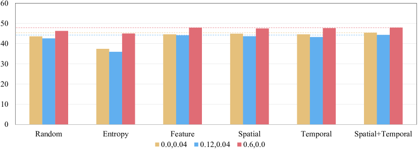
Figure 7: Influence of cost measurement at budget 4800. Dash lines represent the best performing method under different cost measurements (represented by different colors). 0.0,0.04: $c_{f}=0,c_{b}=0.04$; 0.12,0.04: $c_{f}=0.12,c_{b}=0.04$; 0.6,0.0: $c_{f}=0.6,c_{b}=0.0$.

VI-B Limitations

Our proposed method leverages the data collected from the GPS/IMU system to enforce diversity in spatial space. In practice, the quality of the collected data can be affected by device outages, especially for vehicles operating in dense urban areas. Some datasets, e.g. nuScenes, employed additional techniques, e.g. HD map, to guarantee accurate localization, but other datasets, e.g. KITTI, did not. The localization errors may affect the effectiveness of the proposed spatial diversity term. The proposed temporal diversity term and feature diversity term complement spatial diversity and help to alleviate this limitation.

VII Conclusion

In this paper, we explored diversity-based AL for 3D object detection. We proposed a novel acquisition function that enforces diversity in the spatial and temporal space. Extensive experiments on the nuScenes dataset demonstrate that the proposed method outperform the Random and Entropy baseline. To fairly evaluate different AL methods, we propose to measure the annotation cost by taking into consideration both the cost for annotating a frame and a 3D bounding box. We show that how to measure the cost can significantly affect the ranking of the AL strategies and highlight the importance of using realistic cost measurement in evaluating such methods. Finally, we look into the cold-start problem of AL and show that the proposed diversity terms have the advantage of not relying on model prediction, and can be utilized to select better initial batch that not only achieves higher accuracy at early batches, but also results in better performance in the long run. Our work is the pioneering works that investigate AL for 3D object detection in autonomous driving. The proposed acquisition function significantly outperforms the baseline and is applicable to all existing 3D object detectors. The proposed cost measurement scheme provides guidelines for properly evaluating AL methods in the future. Our work provides valuable insights to the AV community and may inspire more studies in this direction.

References

- [1] Z. Yang, Y. Sun, S. Liu, and J. Jia, “3dssd: Point-based 3d single stage object detector,” in Proceedings of the IEEE/CVF conference on computer vision and pattern recognition, 2020, pp. 11 040–11 048.
- [2] B. Zhu, Z. Jiang, X. Zhou, Z. Li, and G. Yu, “Class-balanced grouping and sampling for point cloud 3d object detection,” arXiv preprint arXiv:1908.09492, 2019.
- [3] T. Yin, X. Zhou, and P. Krahenbuhl, “Center-based 3d object detection and tracking,” in Proceedings of the IEEE/CVF Conference on Computer Vision and Pattern Recognition, 2021, pp. 11 784–11 793.
- [4] C. R. Qi, W. Liu, C. Wu, H. Su, and L. J. Guibas, “Frustum pointnets for 3d object detection from rgb-d data,” in Proceedings of the IEEE conference on computer vision and pattern recognition, 2018, pp. 918–927.
- [5] S. Shi, X. Wang, and H. Li, “Pointrcnn: 3d object proposal generation and detection from point cloud,” in The IEEE Conference on Computer Vision and Pattern Recognition (CVPR), June 2019.
- [6] A. H. Lang, S. Vora, H. Caesar, L. Zhou, J. Yang, and O. Beijbom, “Pointpillars: Fast encoders for object detection from point clouds,” in Proceedings of the IEEE/CVF Conference on Computer Vision and Pattern Recognition (CVPR), June 2019.
- [7] Y. Yan, Y. Mao, and B. Li, “Second: Sparsely embedded convolutional detection,” Sensors, vol. 18, no. 10, p. 3337, 2018.
- [8] D. Roth and K. Small, “Margin-based active learning for structured output spaces,” in European Conference on Machine Learning. Springer, 2006, pp. 413–424.
- [9] A. J. Joshi, F. Porikli, and N. Papanikolopoulos, “Multi-class active learning for image classification,” in 2009 IEEE Conference on Computer Vision and Pattern Recognition. IEEE, 2009, pp. 2372–2379.
- [10] D. Yoo and I. S. Kweon, “Learning loss for active learning,” in Proceedings of the IEEE/CVF Conference on Computer Vision and Pattern Recognition, 2019, pp. 93–102.
- [11] O. Sener and S. Savarese, “Active learning for convolutional neural networks: A core-set approach,” arXiv preprint arXiv:1708.00489, 2017.
- [12] L. Lin, K. Wang, D. Meng, W. Zuo, and L. Zhang, “Active self-paced learning for cost-effective and progressive face identification,” IEEE transactions on pattern analysis and machine intelligence, vol. 40, no. 1, pp. 7–19, 2017.
- [13] Y. Yang, Z. Ma, F. Nie, X. Chang, and A. G. Hauptmann, “Multi-class active learning by uncertainty sampling with diversity maximization,” International Journal of Computer Vision, vol. 113, no. 2, pp. 113–127, 2015.
- [14] E. Elhamifar, G. Sapiro, A. Yang, and S. S. Sasrty, “A convex optimization framework for active learning,” in Proceedings of the IEEE International Conference on Computer Vision, 2013, pp. 209–216.
- [15] Y. Guo, “Active instance sampling via matrix partition.” in NIPS, 2010, pp. 802–810.
- [16] Y. Gal and Z. Ghahramani, “Bayesian convolutional neural networks with bernoulli approximate variational inference,” arXiv preprint arXiv:1506.02158, 2015.
- [17] Y. Gal, R. Islam, and Z. Ghahramani, “Deep bayesian active learning with image data,” in International Conference on Machine Learning. PMLR, 2017, pp. 1183–1192.
- [18] Y. Li and Y. Gal, “Dropout inference in bayesian neural networks with alpha-divergences,” in International conference on machine learning. PMLR, 2017, pp. 2052–2061.
- [19] H. H. Aghdam, A. Gonzalez-Garcia, J. v. d. Weijer, and A. M. López, “Active learning for deep detection neural networks,” in Proceedings of the IEEE/CVF International Conference on Computer Vision, 2019, pp. 3672–3680.
- [20] S. Roy, A. Unmesh, and V. P. Namboodiri, “Deep active learning for object detection.” in BMVC, vol. 362, 2018, p. 91.
- [21] C.-C. Kao, T.-Y. Lee, P. Sen, and M.-Y. Liu, “Localization-aware active learning for object detection,” in Asian Conference on Computer Vision. Springer, 2018, pp. 506–522.
- [22] R. Mackowiak, P. Lenz, O. Ghori, F. Diego, O. Lange, and C. Rother, “Cereals-cost-effective region-based active learning for semantic segmentation,” arXiv preprint arXiv:1810.09726, 2018.
- [23] L. Cai, X. Xu, L. Zhang, and C.-S. Foo, “Exploring spatial diversity for region-based active learning,” IEEE Transactions on Image Processing, 2021.
- [24] L. Cai, X. Xu, J. H. Liew, and C. S. Foo, “Revisiting superpixels for active learning in semantic segmentation with realistic annotation costs,” in Proceedings of the IEEE/CVF Conference on Computer Vision and Pattern Recognition, 2021, pp. 10 988–10 997.
- [25] D. Feng, X. Wei, L. Rosenbaum, A. Maki, and K. Dietmayer, “Deep active learning for efficient training of a lidar 3d object detector,” in 2019 IEEE Intelligent Vehicles Symposium (IV). IEEE, 2019, pp. 667–674.
- [26] T. Yuan, F. Wan, M. Fu, J. Liu, S. Xu, X. Ji, and Q. Ye, “Multiple instance active learning for object detection,” in Proceedings of the IEEE/CVF Conference on Computer Vision and Pattern Recognition, 2021, pp. 5330–5339.
- [27] S. V. Desai and V. N. Balasubramanian, “Towards fine-grained sampling for active learning in object detection,” in Proceedings of the IEEE/CVF Conference on Computer Vision and Pattern Recognition Workshops, 2020, pp. 924–925.
- [28] M. Gao, Z. Zhang, G. Yu, S. Ö. Arık, L. S. Davis, and T. Pfister, “Consistency-based semi-supervised active learning: Towards minimizing labeling cost,” in European Conference on Computer Vision. Springer, 2020, pp. 510–526.
- [29] P. Ren, Y. Xiao, X. Chang, P.-Y. Huang, Z. Li, X. Chen, and X. Wang, “A survey of deep active learning,” arXiv preprint arXiv:2009.00236, 2020.
- [30] N. Houlsby, F. Huszár, Z. Ghahramani, and M. Lengyel, “Bayesian active learning for classification and preference learning,” arXiv preprint arXiv:1112.5745, 2011.
- [31] W. H. Beluch, T. Genewein, A. Nürnberger, and J. M. Köhler, “The power of ensembles for active learning in image classification,” in Proceedings of the IEEE Conference on Computer Vision and Pattern Recognition, 2018, pp. 9368–9377.
- [32] M. Hasan and A. K. Roy-Chowdhury, “Context aware active learning of activity recognition models,” in Proceedings of the IEEE International Conference on Computer Vision, 2015, pp. 4543–4551.
- [33] Y.-P. Tang and S.-J. Huang, “Self-paced active learning: Query the right thing at the right time,” in Proceedings of the AAAI conference on artificial intelligence, vol. 33, no. 01, 2019, pp. 5117–5124.
- [34] S. Sinha, S. Ebrahimi, and T. Darrell, “Variational adversarial active learning,” in Proceedings of the IEEE/CVF International Conference on Computer Vision, 2019, pp. 5972–5981.
- [35] C.-A. Brust, C. Käding, and J. Denzler, “Active learning for deep object detection,” arXiv preprint arXiv:1809.09875, 2018.
- [36] W. Liu, D. Anguelov, D. Erhan, C. Szegedy, S. Reed, C.-Y. Fu, and A. C. Berg, “Ssd: Single shot multibox detector,” in European conference on computer vision. Springer, 2016, pp. 21–37.
- [37] S. Shi, X. Wang, and H. P. Li, “3d object proposal generation and detection from point cloud,” in Proceedings of the IEEE Conference on Computer Vision and Pattern Recognition, Long Beach, CA, USA, 2019, pp. 16–20.
- [38] Z. Wang and K. Jia, “Frustum convnet: Sliding frustums to aggregate local point-wise features for amodal 3d object detection,” in 2019 IEEE/RSJ International Conference on Intelligent Robots and Systems (IROS). IEEE, 2019, pp. 1742–1749.
- [39] C. R. Qi, O. Litany, K. He, and L. J. Guibas, “Deep hough voting for 3d object detection in point clouds,” in Proceedings of the IEEE/CVF International Conference on Computer Vision, 2019, pp. 9277–9286.
- [40] C. R. Qi, H. Su, K. Mo, and L. J. Guibas, “Pointnet: Deep learning on point sets for 3d classification and segmentation,” in Proceedings of the IEEE conference on computer vision and pattern recognition, 2017, pp. 652–660.
- [41] C. R. Qi, L. Yi, H. Su, and L. J. Guibas, “Pointnet++: Deep hierarchical feature learning on point sets in a metric space,” arXiv preprint arXiv:1706.02413, 2017.
- [42] Y. Wang, Y. Sun, Z. Liu, S. E. Sarma, M. M. Bronstein, and J. M. Solomon, “Dynamic graph cnn for learning on point clouds,” Acm Transactions On Graphics (tog), vol. 38, no. 5, pp. 1–12, 2019.
- [43] Y. Zhou and O. Tuzel, “Voxelnet: End-to-end learning for point cloud based 3d object detection,” in Proceedings of the IEEE conference on computer vision and pattern recognition, 2018, pp. 4490–4499.
- [44] Q. Chen, L. Sun, Z. Wang, K. Jia, and A. Yuille, “Object as hotspots: An anchor-free 3d object detection approach via firing of hotspots,” in European Conference on Computer Vision. Springer, 2020, pp. 68–84.
- [45] Q. Chen, L. Sun, E. Cheung, and A. L. Yuille, “Every view counts: Cross-view consistency in 3d object detection with hybrid-cylindrical-spherical voxelization,” Advances in Neural Information Processing Systems, 2020.
- [46] X. Chen, H. Ma, J. Wan, B. Li, and T. Xia, “Multi-view 3d object detection network for autonomous driving,” in Proceedings of the IEEE Conference on Computer Vision and Pattern Recognition, 2017.
- [47] S. Vora, A. H. Lang, B. Helou, and O. Beijbom, “Pointpainting: Sequential fusion for 3d object detection,” in Proceedings of the IEEE/CVF Conference on Computer Vision and Pattern Recognition (CVPR), June 2020.
- [48] H. Caesar, V. Bankiti, A. H. Lang, S. Vora, V. E. Liong, Q. Xu, A. Krishnan, Y. Pan, G. Baldan, and O. Beijbom, “nuscenes: A multimodal dataset for autonomous driving,” in Proceedings of the IEEE/CVF Conference on Computer Vision and Pattern Recognition (CVPR), June 2020.
- [49] M. Yuan, H.-T. Lin, and J. Boyd-Graber, “Cold-start active learning through self-supervised language modeling,” arXiv preprint arXiv:2010.09535, 2020.
- [50] A. Holub, P. Perona, and M. C. Burl, “Entropy-based active learning for object recognition,” in 2008 IEEE Computer Society Conference on Computer Vision and Pattern Recognition Workshops. IEEE, 2008.