Optimization of a domestic microgrid equipped with solar panel and battery: Model Predictive Control and Stochastic Dual Dynamic Programming approaches

Abstract

In this study, a microgrid with storage (battery, hot water tank) and solar panel is considered. We benchmark two algorithms, MPC and SDDP, that yield online policies to manage the microgrid, and compare them with a rule based policy. Model Predictive Control (MPC) is a well-known algorithm which models the future uncertainties with a deterministic forecast. By contrast, Stochastic Dual Dynamic Programming (SDDP) models the future uncertainties as stagewise independent random variables with known probability distributions. We present a scheme, based on out-of-sample validation, to fairly compare the two online policies yielded by MPC and SDDP. Our numerical studies put to light that MPC and SDDP achieve significant gains compared to the rule based policy, and that SDDP overperforms MPC not only on average but on most of the out-of-sample assessment scenarios.

Abbreviations
AR	Auto-regressive
EMS	Energy Management System
MPC	Model Predictive Control
SDP	Stochastic Dynamic Programming
SDDP	Stochastic Dual Dynamic Programming
Physical variables
$t$	Time
$\Delta$	Time step (15mn)
$T_{0}$	Horizon (24h)
$p_{t}^{e}$	Electricity price (Euro €)
$p_{t}^{d}$	Thermal comfort (virtual price)
$A_{p}$	Surface of solar panel ($m^{2}$)
$\rho_{c}$	Battery charge rate
$\rho_{d}$	Battery discharge rate
$\beta_{h}$	Conversion yield for hot water tank
Decision variables and uncertainties
$(\Omega,\mathcal{F},\mathbb{P})$	Probability space
$\boldsymbol{B^{\textstyle\text{\unboldmath$\scriptstyle$}}_{\textstyle\text{\unboldmath$\scriptstyle t$}}}$	Level of energy in battery (kWh)
$\boldsymbol{H^{\textstyle\text{\unboldmath$\scriptstyle$}}_{\textstyle\text{\unboldmath$\scriptstyle t$}}}$	Level of energy in hot water tank (kWh)
$\mathbf{D}^{el}_{t}$	Electrical demand (kW)
$\mathbf{D}^{th}_{t}$	Hot water demand (kW)
$\boldsymbol{\Phi}^{pv}_{t}$	Production of the solar panel (kW)
$\theta_{t}^{i}$	Inner temperature (${}^{\circ}C$)
$\theta_{t}^{w}$	Walls temperature (${}^{\circ}C$)
$\theta_{t}^{e}$	Outdoor temperature (${}^{\circ}C$)
$\boldsymbol{F^{\textstyle\text{\unboldmath$\scriptstyle b$}}_{\textstyle\text{\unboldmath$\scriptstyle t$}}}$	Energy exchanged with the battery (kW)
$\boldsymbol{F^{\textstyle\text{\unboldmath$\scriptstyle w$}}_{\textstyle\text{\unboldmath$\scriptstyle t$}}}$	Energy injected in the hot water tank (kW)
$\boldsymbol{F^{\textstyle\text{\unboldmath$\scriptstyle h$}}_{\textstyle\text{\unboldmath$\scriptstyle t$}}}$	Energy injected in the electrical heater (kW)
$\boldsymbol{U^{\textstyle\text{\unboldmath$\scriptstyle$}}_{\textstyle\text{\unboldmath$\scriptstyle t$}}}=(\boldsymbol{F^{\textstyle\text{\unboldmath$\scriptstyle b$}}_{\textstyle\text{\unboldmath$\scriptstyle t$}}},\boldsymbol{F^{\textstyle\text{\unboldmath$\scriptstyle w$}}_{\textstyle\text{\unboldmath$\scriptstyle t$}}},\boldsymbol{F^{\textstyle\text{\unboldmath$\scriptstyle h$}}_{\textstyle\text{\unboldmath$\scriptstyle t$}}})$	Controls
$\boldsymbol{W^{\textstyle\text{\unboldmath$\scriptstyle$}}_{\textstyle\text{\unboldmath$\scriptstyle t$}}}=(\mathbf{D}^{el}_{t},\mathbf{D}^{th}_{t},\boldsymbol{\Phi}^{pv}_{t})$	Uncertainties
$\boldsymbol{X^{\textstyle\text{\unboldmath$\scriptstyle$}}_{\textstyle\text{\unboldmath$\scriptstyle t$}}}=(\boldsymbol{B^{\textstyle\text{\unboldmath$\scriptstyle$}}_{\textstyle\text{\unboldmath$\scriptstyle t$}}},\boldsymbol{H^{\textstyle\text{\unboldmath$\scriptstyle$}}_{\textstyle\text{\unboldmath$\scriptstyle t$}}},\boldsymbol{\theta}^{w}_{t},\boldsymbol{\theta}^{i}_{t})$	States
Mappings
$f_{t}:\mathbb{X}_{t}\times\mathbb{U}_{t}\times\mathbb{W}_{t+1}\rightarrow\mathbb{X}_{t+1}$	Linear dynamics
$L_{t}:\mathbb{X}_{t}\times\mathbb{U}_{t}\times\mathbb{W}_{t+1}\rightarrow\mathbb{R}$	Convex operational cost
$K:\mathbb{X}_{T}\rightarrow\mathbb{R}$	Convex final cost
$\pi_{t}:\mathbb{X}_{t}\rightarrow\mathbb{U}_{t}$	Control policy

Table 1: Nomenclature

1 Introduction

1.1 Background introduction

A microgrid is a local energy network that produces part of its energy and controls its own demand. Such systems are complex to control because, on the one hand, of the different stocks and interconnections, and, on the other hand, of electrical demands and weather conditions (heat demand and renewable energy production) that are highly variable and hard to predict at local scale (see [1, 2] for a panorama of the challenges faced when controlling microgrids).

We consider here a domestic microgrid equipped with a battery, an electrical hot water tank and a solar panel, as in Figure 1. The microgrid is connected to an external grid to import electricity when needed. The battery stores energy when external grid prices are low or when the production of the solar panel is above the electrical demand. The house’s envelope also plays the role of heat storage. As a consequence, the system has four stocks to store energy: a battery, a hot water tank, and two passive stocks being the house’s walls and inner rooms. Two kinds of uncertainties affect the system: the electrical and domestic hot water demands are not known in advance; the production of the solar panel is substantially perturbed by the variable weather nebulosity.

We aim to compare two classes of algorithms to tackle uncertainties in a microgrid Energy Management System (EMS). The Model Predictive Control (MPC) algorithm (or its stochastic variant, Stochastic Model Predictive Control) relies on a mathematical representation of the future uncertainties as deterministic forecasts; then, MPC computes decisions online as solutions of a deterministic multistage optimization problem. Stochastic Dual Dynamic Programming (SDDP) relies on a mathematical representation of the future uncertainties as stagewise independent random variables with known probability distributions; then, SDDP computes offline a set of value functions by backward induction, and computes online decisions as solutions of a single stage stochastic optimization problem, using the value functions. We present a fair comparison of these two algorithms, and highlight the pros and cons of both methods.

1.2 Literature review

Optimization and energy management systems

EMS are integrated automated tools used to monitor and control energy systems. In [1], the authors give an overview of the use of optimization methods in the design of EMS. The MPC algorithm [3] and its stochastic variant, Stochastic Model Predictive Control (SMPC) [4], have been widely used to control EMS. We refer the reader to [5] for applications of MPC in buildings. In [6], the authors use MPC for the optimal control of a domestic microgrid, and investigate how to balance the uncertainties of renewable energies with the microgrid. In [7], the authors apply SMPC to the management of an isolated microgrid, and highlight the benefit of this method; an application of SMPC in buildings is presented in [8]; a variant based on robust optimization is proposed in [9].

Stochastic optimization

At local scale, electrical demand and production are highly variable, especially as microgrids are expected to absorb renewable energies. This leads to pay attention to stochastic optimization approaches [10]. Stochastic optimization has been widely applied to hydrovalleys management [11]. Other applications have arisen recently, such as integration of wind energy and storage [12] or insulated microgrids management [13, 14].

Stochastic Dynamic Programming (SDP) [15] is a general method to solve stochastic optimal control problems. In energy applications, a variant of SDP, Stochastic Dual Dynamic Programming (SDDP), has demonstrated its adequacy for large scale convex applications. SDDP was first described in the seminal paper [11]; we refer to [16] for a generic description of the algorithm and its application to the management of hydrovalleys; a proof of convergence in the linear case is given in [17], and in the convex case in [18]. Recent articles have applied SDDP to the management of energy systems. In [19], numerical experiments show that SDDP yields better results than a myopic policy. In [20], SDDP is applied to the dispatch of energy inside the German national grid, under time correlated uncertainties; the authors observe that SDDP achieves better performances than those of a deterministic-based policy. Other Approximate Dynamic Programming algorithms have been designed to tackle different stochastic optimal control problems like, for instance, incorporating probability constraints [21].

1.3 Main contributions and structure of the paper

We provide a rigorous mathematical formulation of the optimal management of a domestic microgrid — equipped with a battery, an electrical hot water tank and a solar panel, and connected to an external supply network — under stochasticity of demand and of renewable energy production. To manage the microgrid, we design online policies using two different algorithms, MPC and SDDP. Then, we develop a fair benchmark methodology to compare the two algorithms, based on a realistic use case. The comparison reveals that SDDP overperforms MPC not only on average but, interestingly, on most of the out-of-sample assessment scenarios.

The paper is organized as follows. In Sect. 2, we detail the modeling of a small residential microgrid and formulate a mathematical multistage stochastic optimization problem. Then, we outline the two algorithms, MPC and SDDP, in Sect. 3. Finally, in Sect. 4 we detail the benchmark methodology and we provide numerical results on the systematic comparison of MPC, SDDP and a rule based policy. Sect. 5 concludes and the Appendix 6 provides details on the physical equations of the microgrid.

2 Optimization problem statement

We consider the optimal management of a microgrid which, as depicted in Figure 1, consists of a single house equipped with a battery and an electrical hot water tank. An electrical heater can produce heat in winter, and a solar panel can produce energy locally. The decision maker aims at minimizing the energy bill — that is, the cost of the possible recourse energy supplied by the external network — while satisfying the energy demands (hot water and electricity), and ensuring a minimal thermal comfort.

In this section, we write up a multistage stochastic optimization problem. As decisions are taken at discrete time steps, we start by discretizing the time interval in §2.1. Then, we introduce the uncertainties in §2.2, the controls and the stocks in §2.3 and §2.4. We detail the nonanticipativity constraints in §2.5, the bounds constraints in §2.6 and the objective function in §2.7. Finally, we formulate a multistage stochastic optimization problem in §2.8.

Figure 1: Electrical microgrid

2.1 Decisions are taken at discrete time steps

The EMS takes decisions every 15 minutes to control the system. We consider a time interval $\Delta=15\text{mn}$, a time horizon $T_{0}{=}24\text{h}$ and a number $T{=}T_{0}/\Delta{=}96$ of time steps. We adopt the following convention for discrete time processes: for each time step $t\in\{0,1,\cdots,T\}$, $x_{t}$ denotes the value of the variable $x$ at the beginning of the interval $[t\Delta,(t+1)\Delta)$. Otherwise stated, we will denote by $[t,t+1)$ the continuous time interval $[t\Delta,(t+1)\Delta)$.

2.2 Modeling uncertainties as random variables

Because of their unpredictable nature, the EMS cannot anticipate the values of electrical and thermal demands, nor the production of the solar panel. We choose to model these quantities as random variables over a probability space $(\Omega,\mathcal{F},\mathbb{P})$. We adopt the following convention: a random variable will be denoted by an uppercase bold letter $\boldsymbol{Z^{\textstyle\text{\unboldmath$\scriptstyle$}}_{\textstyle\text{\unboldmath$\scriptstyle$}}}$, and its realization for a given outcome $\omega\in\Omega$ will be denoted in lowercase $z=\boldsymbol{Z^{\textstyle\text{\unboldmath$\scriptstyle$}}_{\textstyle\text{\unboldmath$\scriptstyle$}}}(\omega)$. We denote by $\mathbf{D}^{el}_{t}$ the electrical demand, $\mathbf{D}^{th}_{t}$ the hot water demand and $\boldsymbol{\Phi}^{pv}_{t}$ the production of the solar panel, all being real-valued random variables. For each time step $t=1,\ldots,T$, we define the (uncertainty) random variable

$$\boldsymbol{W}_{t}=(\mathbf{D}^{el}_{t},\mathbf{D}^{th}_{t},\boldsymbol{\Phi}^{pv}_{t})\;.$$ (1)

The uncertainty $\boldsymbol{W}_{t}$ is a multivariate random variable taking values in $\mathbb{W}_{t}=\mathbb{R}^{3}$.

2.3 Modeling controls as random variables

As decisions depend on the previous uncertainties, controls are random variables. At the beginning of the time interval $[t,t+1)$, the EMS takes three decisions:

• $\boldsymbol{F^{\textstyle\text{\unboldmath$\scriptstyle b$}}_{\textstyle\text{\unboldmath$\scriptstyle t$}}}$, how much energy to charge in/discharge from the battery,

• $\boldsymbol{F^{\textstyle\text{\unboldmath$\scriptstyle w$}}_{\textstyle\text{\unboldmath$\scriptstyle t$}}}$, how much energy to store in the electrical hot water tank,

• $\boldsymbol{F^{\textstyle\text{\unboldmath$\scriptstyle h$}}_{\textstyle\text{\unboldmath$\scriptstyle t$}}}$, how much energy to inject in the electrical heater,

during the time interval $[t,t+1)$. For each time step $t=1,\ldots,T$, we define the decision multivariate random variable, taking values in $\mathbb{U}_{t}=\mathbb{R}^{3}$, as

$$\boldsymbol{U}_{t}=(\boldsymbol{F^{\textstyle\text{\unboldmath$\scriptstyle b$}}_{\textstyle\text{\unboldmath$\scriptstyle t$}}},\boldsymbol{F^{\textstyle\text{\unboldmath$\scriptstyle w$}}_{\textstyle\text{\unboldmath$\scriptstyle t$}}},\boldsymbol{F^{\textstyle\text{\unboldmath$\scriptstyle h$}}_{\textstyle\text{\unboldmath$\scriptstyle t$}}})\;.$$ (2)

During the time interval $[t,t+1)$, the EMS imports an energy quantity $\boldsymbol{F^{\textstyle\text{\unboldmath$\scriptstyle ne$}}_{\textstyle\text{\unboldmath$\scriptstyle{t+1}$}}}$ from the external network in order to fulfill the load balance equation

$$\boldsymbol{F^{\textstyle\text{\unboldmath$\scriptstyle ne$}}_{\textstyle\text{\unboldmath$\scriptstyle{t+1}$}}}+\boldsymbol{\Phi}^{pv}_{t+1}=\boldsymbol{F^{\textstyle\text{\unboldmath$\scriptstyle b$}}_{\textstyle\text{\unboldmath$\scriptstyle t$}}}+\boldsymbol{F^{\textstyle\text{\unboldmath$\scriptstyle w$}}_{\textstyle\text{\unboldmath$\scriptstyle t$}}}+\boldsymbol{F^{\textstyle\text{\unboldmath$\scriptstyle h$}}_{\textstyle\text{\unboldmath$\scriptstyle t$}}}+\mathbf{D}^{el}_{t+1}\;,$$ (3)

whatever the demand $\mathbf{D}^{el}_{t+1}$ and the production of the solar panel $\boldsymbol{\Phi}^{pv}_{t+1}$, unknown at the beginning of the time interval $[t,t+1)$. On the left-hand side of Equation (3), the load consists of

• $\boldsymbol{F^{\textstyle\text{\unboldmath$\scriptstyle ne$}}_{\textstyle\text{\unboldmath$\scriptstyle{t+1}$}}}$, the energy surplus or shortage (when $\boldsymbol{F^{\textstyle\text{\unboldmath$\scriptstyle ne$}}_{\textstyle\text{\unboldmath$\scriptstyle{t+1}$}}}<0$, one wastes the surplus; when $\boldsymbol{F^{\textstyle\text{\unboldmath$\scriptstyle ne$}}_{\textstyle\text{\unboldmath$\scriptstyle{t+1}$}}}>0$, one imports the shortage from the network),

• $\boldsymbol{\Phi}^{pv}_{t+1}$, the production of the solar panel,

all during the time interval $[t,t+1)$. On the right-hand side of Equation (3), the electrical demand is the sum of

• $\boldsymbol{F^{\textstyle\text{\unboldmath$\scriptstyle b$}}_{\textstyle\text{\unboldmath$\scriptstyle t$}}}$, the energy exchanged with the battery,

• $\boldsymbol{F^{\textstyle\text{\unboldmath$\scriptstyle w$}}_{\textstyle\text{\unboldmath$\scriptstyle t$}}}$, the energy injected into the electrical hot water tank,

• $\boldsymbol{F^{\textstyle\text{\unboldmath$\scriptstyle h$}}_{\textstyle\text{\unboldmath$\scriptstyle t$}}}$, the energy injected in the electrical heater,

• $\boldsymbol{D^{\textstyle\text{\unboldmath$\scriptstyle el$}}_{\textstyle\text{\unboldmath$\scriptstyle{t+1}$}}}$, the electrical demands (lightning, cooking…), aggregated in a single demand,

all during the time interval $[t,t+1)$.

Later, we will aggregate the solar panel production $\boldsymbol{\Phi}^{pv}_{t+1}$ with the demands $\mathbf{D}^{el}_{t+1}$ in Equation (3), as these two quantities appear only by their difference.

2.4 States and dynamics

The state is the multivariate random variable

$$\boldsymbol{X}_{t}=(\boldsymbol{B^{\textstyle\text{\unboldmath$\scriptstyle$}}_{\textstyle\text{\unboldmath$\scriptstyle t$}}},\boldsymbol{H^{\textstyle\text{\unboldmath$\scriptstyle$}}_{\textstyle\text{\unboldmath$\scriptstyle t$}}},\boldsymbol{\theta}^{w}_{t},\boldsymbol{\theta}^{i}_{t})\;,$$ (4)

which consists of the stocks $\boldsymbol{B^{\textstyle\text{\unboldmath$\scriptstyle$}}_{\textstyle\text{\unboldmath$\scriptstyle t$}}}$ in the battery and $\boldsymbol{H^{\textstyle\text{\unboldmath$\scriptstyle$}}_{\textstyle\text{\unboldmath$\scriptstyle t$}}}$ in the electrical hot water tank, plus the two temperatures $(\boldsymbol{\theta}^{w}_{t},\boldsymbol{\theta}^{i}_{t})$ of the thermal envelope. Thus, the state random variable $\boldsymbol{X}_{t}$ takes values in $\mathbb{X}_{t}=\mathbb{R}^{4}$.

The discrete time dynamics $f_{t}:\mathbb{X}_{t}\times\mathbb{U}_{t}\times\mathbb{W}_{t+1}\rightarrow\mathbb{X}_{t+1}$ describes the time evolution

$$\boldsymbol{X}_{t+1}=f_{t}\big{(}\boldsymbol{X}_{t},\boldsymbol{U}_{t},\boldsymbol{W}_{t+1}\big{)}$$ (5)

of the state, where $f_{t}$ is a piecewise linear function (a property that will prove important for the SDDP algorithm), that corresponds to the integration of the continuous dynamics (21)-(22)-(24) given in Appendix 6. We suppose that we start from a given state $x_{0}\in\mathbb{X}_{0}=\mathbb{R}^{4}$, thus adding the constraint $\boldsymbol{X}_{0}=x_{0}$.

2.5 Nonanticipativity constraints

The future realizations of uncertainties are unknown. Thus, decisions at time step $t$ are functions of previous history only, that is, the information collected between step $0$ and step $t$. Such a constraint is encoded as an algebraic constraint, using the tools of Probability theory [22], in the so-called nonanticipativity constraints written as

$$\sigma(\boldsymbol{U}_{t})\subset\mathcal{F}_{t}\;,$$ (6a)

where $$\sigma(\boldsymbol{U}_{t}) \sigma \boldsymbol{U}_{t} \mathcal{F}_{t}=\sigma(\boldsymbol{W}_{1},\cdots,\boldsymbol{W}_{t}) \sigma (\boldsymbol{W}_{1}, \ldots,\boldsymbol{W}_{t}) \pi_{t}:\mathbb{W}_{1}\times\dots\times\mathbb{W}_{t}\rightarrow\mathbb{U}_{t}$$ is the -algebra generated by the random variable  and is the -algebra generated by the previous uncertainties  . If Constraint (6a) holds true, the Doob Lemma [22] ensures that there exists a measurable function such that

$$\boldsymbol{U}_{t}=\pi_{t}(\boldsymbol{W}_{1},\ldots,\boldsymbol{W}_{t})\;.$$ (6b)

This is how we turn an (abstract) algebraic constraint into a more practical functional constraint. The function $\pi_{t}$ is called a policy.

2.6 Bounds constraints

The stocks $\boldsymbol{B^{\textstyle\text{\unboldmath$\scriptstyle$}}_{\textstyle\text{\unboldmath$\scriptstyle t$}}}$ in the battery and $\boldsymbol{H^{\textstyle\text{\unboldmath$\scriptstyle$}}_{\textstyle\text{\unboldmath$\scriptstyle t$}}}$ in the tank are bounded:

$$\underline{b}\leq\boldsymbol{B^{\textstyle\text{\unboldmath$\scriptstyle$}}_{\textstyle\text{\unboldmath$\scriptstyle t$}}}\leq\overline{b}\;,\enspace 0\leq\boldsymbol{H^{\textstyle\text{\unboldmath$\scriptstyle$}}_{\textstyle\text{\unboldmath$\scriptstyle t$}}}\leq\overline{h}\;.$$ (7)

At time step $t$, the control $\boldsymbol{F^{\textstyle\text{\unboldmath$\scriptstyle b$}}_{\textstyle\text{\unboldmath$\scriptstyle t$}}}$ must ensure that the next state $\boldsymbol{B^{\textstyle\text{\unboldmath$\scriptstyle$}}_{\textstyle\text{\unboldmath$\scriptstyle{t+1}$}}}$ is admissible, that is, satisfies $\underline{b}\leq\boldsymbol{B^{\textstyle\text{\unboldmath$\scriptstyle$}}_{\textstyle\text{\unboldmath$\scriptstyle{t+1}$}}}\leq\overline{b}$, which, by time discretization of (21), is equivalent to the two inequalities

$$\underline{b}\leq\boldsymbol{B^{\textstyle\text{\unboldmath$\scriptstyle$}}_{\textstyle\text{\unboldmath$\scriptstyle t$}}}+\Delta\Big{[}\rho_{c}(\boldsymbol{F^{\textstyle\text{\unboldmath$\scriptstyle b$}}_{\textstyle\text{\unboldmath$\scriptstyle t$}}})^{+}+\dfrac{1}{\rho_{d}}(\boldsymbol{F^{\textstyle\text{\unboldmath$\scriptstyle b$}}_{\textstyle\text{\unboldmath$\scriptstyle t$}}})^{-}\Big{]}\leq\overline{b}\;,$$ (8)

with $\rho_{c}$ and $\rho_{d}$ being the charge and discharge efficiencies of the battery. Thus, the constraints on $\boldsymbol{F^{\textstyle\text{\unboldmath$\scriptstyle b$}}_{\textstyle\text{\unboldmath$\scriptstyle t$}}}$ depends on the stock $\boldsymbol{B^{\textstyle\text{\unboldmath$\scriptstyle$}}_{\textstyle\text{\unboldmath$\scriptstyle t$}}}$. The same reasoning applies for the tank energy $\boldsymbol{F^{\textstyle\text{\unboldmath$\scriptstyle w$}}_{\textstyle\text{\unboldmath$\scriptstyle t$}}}$ and the stock $\boldsymbol{H^{\textstyle\text{\unboldmath$\scriptstyle$}}_{\textstyle\text{\unboldmath$\scriptstyle t$}}}$. Furthermore, we set bound constraints on controls:

$$-\overline{f}^{b}\leq\boldsymbol{F^{\textstyle\text{\unboldmath$\scriptstyle b$}}_{\textstyle\text{\unboldmath$\scriptstyle t$}}}\leq\overline{f}^{b}\;,\enspace 0\leq\boldsymbol{F^{\textstyle\text{\unboldmath$\scriptstyle w$}}_{\textstyle\text{\unboldmath$\scriptstyle t$}}}\leq\overline{f}_{t}^{w}\;,\enspace 0\leq\boldsymbol{F^{\textstyle\text{\unboldmath$\scriptstyle h$}}_{\textstyle\text{\unboldmath$\scriptstyle t$}}}\leq\overline{f}_{t}^{h}\;.$$ (9)

Finally, the load-balance equation (3) also acts as a constraint on the controls. We gather all these constraints into an admissible subset $\mathcal{U}^{ad}_{t}(\boldsymbol{X}_{t})$ of $\mathbb{U}_{t}=\mathbb{R}^{3}$, depending on the current state $\boldsymbol{X}_{t}$, giving the constraint

$$\boldsymbol{U}_{t}\in\mathcal{U}^{ad}_{t}(\boldsymbol{X}_{t})\;.$$ (10)

Note that we do not enforce any explicit bounds on the inner temperature. Instead, we choose to add a penalization term in the objective function if the temperature is below a given threshold, as explained below.

2.7 Objective function

At time step $t$, the instantaneous cost $L_{t}:\mathbb{X}_{t}\times\mathbb{U}_{t}\times\mathbb{W}_{t+1}\rightarrow\mathbb{R}$ aggregates two different costs as in the formula

$$L_{t}(x_{t},u_{t},w_{t+1})=p^{e}_{t}\times\max\{0,f^{ne}_{t+1}\}+p^{d}_{t}\times\max\{0,\overline{\theta^{i}_{t}}-\theta^{i}_{t}\}\;,$$ (11)

where $f^{ne}_{t+1}$ is a function of $(u_{t},w_{t+1})$ by (3), and $\theta^{i}_{t}$ is part of the state $x_{t}$ in (4).

First, one pays a unitary price $p_{t}^{e}$ to import electricity from the external network between step $t$ and $t+1$; hence, the electricity cost is equal to $p^{e}_{t}\times\max\{0,f^{ne}_{t+1}\}$. Second, if the indoor temperature is below a given threshold, we penalize the induced discomfort with a cost $p^{d}_{t}\times\max\{0,\overline{\theta^{i}_{t}}-\theta^{i}_{t}\}$, where $p_{t}^{d}$ is a virtual price of discomfort (we choose not to penalize the temperature in case it is above a given threshold, as we do not consider any air conditioning in this study). The cost $L_{t}$ is a convex piecewise linear function, a property that will prove important for the SDDP algorithm. To ensure that stocks are not empty at the final time step $T$, we add a convex piecewise linear final cost $K:\mathbb{X}_{T}\rightarrow\mathbb{R}$ of the form

$$K(x_{T})=\kappa\times\max\{0,x_{0}-x_{T}\}\;,$$ (12)

where $\kappa$ is a positive penalization coefficient (calibrated by trial and error).

As decisions $\boldsymbol{U}_{t}$ and states $\boldsymbol{X}_{t}$ are random, the costs $L_{t}(\boldsymbol{X}_{t},\boldsymbol{U}_{t},\boldsymbol{W}_{t+1})$ and $K(\boldsymbol{X}_{T})$ become also random variables. We choose to minimize the expected value of the daily operational cost, that is,

$$\mathbb{E}\Bigg{[}\sum_{t=0}^{T-1}L_{t}(\boldsymbol{X}_{t},\boldsymbol{U}_{t},\boldsymbol{W}_{t+1})+K(\boldsymbol{X}_{T})\Bigg{]}\;,$$ (13)

yielding the expected value of a convex piecewise linear cost.

2.8 Stochastic optimal control formulation

Finally, the EMS problem is written as a stochastic optimal control problem

$$\underset{\boldsymbol{X},\boldsymbol{U}}{\min}\leavevmode\nobreak\ \mathbb{E}\;\Bigg{[}\sum_{t=0}^{T-1}L_{t}(\boldsymbol{X}_{t},\boldsymbol{U}_{t},\boldsymbol{W}_{t+1})+K(\boldsymbol{X}_{T})\Bigg{]}\;,$$ (14a)

s.t. $$\boldsymbol{X}_{t+1}=f_{t}\big{(}\boldsymbol{X}_{t},\boldsymbol{U}_{t},\boldsymbol{W}_{t+1}\big{)}\;,\enspace\boldsymbol{X}_{0}=x_{0}\;,\enspace t=0,\ldots,T-1\;,$$ (14b)

$$\boldsymbol{U}_{t}\in\mathcal{U}^{ad}_{t}(\boldsymbol{X}_{t})\;,\enspace t=0,\ldots,T-1\;,$$ (14c)

$$\sigma(\boldsymbol{U}_{t})\subset\mathcal{F}_{t}\;,\enspace t=0,\ldots,T-1\;.$$ (14d)

Problem (14) expresses that the microgrid manager aims to minimize the expected value of the costs while satisfying the dynamics, the control bounds and the nonanticipativity constraints.

3 Resolution methods

The exact resolution of Problem (14) is out of reach in general. We propose two different algorithms that provide policies $\pi_{t}:\mathbb{W}_{1}\times\cdots\times\mathbb{W}_{t}\rightarrow\mathbb{U}_{t}$ that map available information $w_{1},\ldots,w_{t}$ at step $t$ to a decision $u_{t}$.

In §3.1, we start by presenting how to design management policies with the MPC algorithm. Then, we depict SDDP-based policies in §3.2. Both methods use the dynamics $f_{t}$ in (5), the constraints sets $\mathcal{U}^{ad}_{t}(\cdot)$ in (10), and the cost functions $L_{t}$ in (11) and $K$ in (12).

3.1 Model Predictive Control (MPC)

Be it ordinary or stochastic, MPC is a classical algorithm that is commonly used to solve stochastic optimization problems. Regarding MPC, we follow [15]. At time step $t$, we consider a deterministic forecast $(\overline{w}_{t+1},\ldots,\overline{w}_{T})$ of the future uncertainties $(\boldsymbol{W}_{t+1},\ldots,\boldsymbol{W}_{T})$ (see §6.4 for more details) and we solve the following deterministic problem, where the state $x_{t}$ is given:

$$\underset{(u_{t},\cdots,u_{T-1})}{\min}\leavevmode\nobreak\ \sum_{j=t}^{T-1}L_{j}(x_{j},u_{j},\overline{w}_{j+1})+K(x_{T})\;,$$ (15a)

s.t. $$x_{j+1}=f_{j}\big{(}x_{j},u_{j},\overline{w}_{j+1}\big{)}\;,\enspace j=t,\ldots,T-1\;,$$ (15b)

$$u_{j}\in\mathcal{U}^{ad}_{j}(x_{j})\;,\enspace j=t,\ldots,T-1\;.$$ (15c)

Then, we retrieve the optimal decisions $(u_{t}^{\sharp},\ldots,u_{T-1}^{\sharp})$ and only keep the first decision $u_{t}^{\sharp}$ to control the system at the beginning of the time interval $[t,t+1)$. This procedure is then restarted at step $t+1$. Thus, MPC solves an optimization problem at each time step, with a time span going from the current time step $t$ to the final time step $T$. Then, at the next time $t+1$, the optimizer updates the scenario $(\overline{w}_{t+1},\ldots,\overline{w}_{T})$ to take into account the latest observation made at $t+1$.

3.2 Stochastic Dual Dynamic Programming (SDDP)

As said in §1.2, SDDP is an algorithm widely used to optimize energy systems. The SDDP algorithm provides, at each time step, a value function and an online control policy. Whereas the value functions are computed offline (hence with offline data), online control policies are computed taking into account an online probability distribution on the next period noise.

Dynamic Programming and Bellman principle

The Dynamic Programming method [23] provides solutions of Problem (14) as state feedbacks $\pi_{t}:\mathbb{X}_{t}\rightarrow\mathbb{U}_{t}$ (these feedbacks are optimal when the noise process is made of independent random variables). Dynamic Programming makes use of a sequence of value functions, obtained offline by setting $V_{T}(x_{T})=K(x_{T})$ and by solving backward in time the recursive functional equations

$$V_{t}(x_{t})=\min_{u\in\mathcal{U}^{ad}_{t}(x_{t})}\int_{\mathbb{W}_{t+1}}\Big{[}L_{t}(x_{t},u,w_{t+1})+\\ V_{t+1}\big{(}f_{t}(x_{t},u,w_{t+1})\big{)}\Big{]}\mu^{of}_{t+1}(dw_{t+1})\;,$$ (16)

where $\mu^{of}_{t+1}$ is a (offline) probability distribution on $\mathbb{W}_{t+1}$. Once these functions obtained, we compute a decision at time step $t$ as a state feedback

$$\pi_{t}(x_{t})\in\mathop{\arg\min}_{u\in\mathcal{U}^{ad}_{t}(x_{t})}\int_{\mathbb{W}_{t+1}}\Big{[}L_{t}(x_{t},u,w_{t+1})+\\ V_{t+1}\big{(}f_{t}(x_{t},u,w_{t+1})\big{)}\Big{]}\mu^{on}_{t+1}(dw_{t+1})\;,$$ (17)

where $\mu_{t+1}^{on}$ is an online probability distribution on $\mathbb{W}_{t+1}$. This method proves to be optimal when the random variables $\boldsymbol{W}_{1},\ldots,\boldsymbol{W}_{T}$ are stagewise independent and when $\mu^{on}_{t}=\mu^{of}_{t}$ is the probability distribution of $\boldsymbol{W}_{t}$.

Description of Stochastic Dual Dynamic Programming

Dynamic Programming suffers from the well-known curse of dimensionality [23]: its numerical resolution fails for state dimension typically greater than 4 when value functions are computed on a numerical grid. When uncertainties are stagewise independent random variables, costs $L_{t}$ and $K$ are convex and dynamics $f_{t}$ are linear, the SDDP algorithm provides a solution to Problem (14) where the value functions are represented by convex polyhedral functions [18]. Most achievements of SDDP have been obtained in the linear case — when all the costs are linear — as each subproblem (16) can be solved with the simplex algorithm. However, the extension to the generic convex case has not been studied extensively.

SDDP provides an outer approximation of the value function $V_{t}$ in (16). Provided a bundle of $k$ supporting hyperplanes $\{(\lambda^{j}_{t},\beta^{j}_{t})\}_{j=1,\cdots,k}$ (with, for each $j=1,\cdots,k$, $\lambda^{j}_{t}\in\mathbb{R}^{4}$ and $\beta^{j}_{t}\in\mathbb{R}$), the corresponding outer approximation $\underline{V}_{t}^{k}$ is given by

$$\underline{V}_{t}^{k}(x_{t}) =\min_{\varrho_{t}\in\mathbb{R}}\varrho_{t}\;,$$ (18a)

s.t. $$\big{\langle}\lambda_{t}^{j}\>,x_{t}\big{\rangle}+\beta_{t}^{j}\leq\varrho_{t}\;,\enspace\forall j=1,\cdots,k\;.$$ (18b)

SDDP takes as input an initial value function $\underline{V}_{t+1}^{0}$ (usually $-\infty$) and an initial state $x_{0}$. In the algorithm, we assume that the probability distributions have finite support $\{w_{t+1}^{1},\ldots,w_{t+1}^{S}\}$. The offline distribution $\mu_{t+1}^{of}$ is then written in the form $\mu_{t+1}^{of}=\sum_{s=1}^{S}p_{t+1}^{s}\delta_{w_{t+1}^{s}}$, where $\delta_{w_{t+1}^{s}}$ is the Dirac measure at $w_{t+1}^{s}$ and $p_{t+1}^{1},\ldots,p_{t+1}^{S}$ are probability weights. Then, each iteration $k$ of SDDP encompasses two passes.

• During the forward pass, we draw a scenario $w_{1}^{k},\ldots,w_{T}^{k}$ of uncertainties, and obtain a state trajectory $\big{\{}x_{t}^{k}\big{\}}_{t=0\cdots T}$ along this scenario as follows. Starting from initial state $x_{0}$, we compute $x_{t+1}^{k}$ from $x_{t}^{k}$ in an iterative fashion: i) we obtain a control $u_{t}^{k}$ at time step $t$, using the available $\underline{V}_{t+1}^{k}$ function, by

  $$u_{t}^{k}\in\mathop{\arg\min}_{u\in\mathcal{U}^{ad}_{t}(x_{t})}\sum_{i=1}^{S}p_{t+1}^{i}\big{[}L_{t}(x_{t}^{k},u,w_{t+1}^{i})+\underline{V}_{t+1}^{k}\big{(}f_{t}(x_{t}^{k},u,w_{t+1}^{i})\big{)}\big{]}\;,$$ (19a)

  and ii), we set $$x_{t+1}^{k}=f_{t}(x_{t}^{k},u_{t}^{k},w_{t+1}^{k}) f_{t}$$ where is the piecewise linear dynamics in (5).

• During the backward pass, we update the approximated value functions $\big{\{}\underline{V}_{t}^{k}\big{\}}_{t=0,\cdots,T}$ backward in time along the trajectory $\big{\{}x_{t}^{k}\big{\}}_{t=0,\cdots,T}$. At time step $t$, we solve the problem

  $$\varrho_{t}^{k+1}=\min_{u\in\mathcal{U}^{ad}_{t}(x_{t})}\sum_{i=1}^{S}p_{t+1}^{i}\big{[}L_{t}(x_{t}^{k},u,w_{t+1}^{i})+\underline{V}_{t+1}^{k+1}\big{(}f_{t}(x_{t}^{k},u,w_{t+1}^{i})\big{)}\big{]}\;,$$ (19b)

  and we obtain a new cut $(\lambda_{t}^{k+1},\beta_{t}^{k+1})$ where $\lambda_{t}^{k+1}$ is a subgradient of the optimal cost function (19b) evaluated at the point $x_{t}=x_{t}^{k}$,

  $$\lambda_{t}^{k+1}\in\sum_{i=1}^{S}p_{t+1}^{i}\big{[}\partial_{x}L_{t}(x_{t}^{k},u_{t}^{k+1},w_{t+1}^{i})+\\ \partial_{x}\underline{V}_{t+1}^{k+1}\big{(}f_{t}(x_{t}^{k},u_{t}^{k+1}w_{t+1}^{i})\big{)}\big{]}\;,$$

  and where $\beta_{t}^{k+1}=\varrho_{t}^{k+1}-\big{\langle}\lambda_{t}^{k+1}\>,x_{t}^{k}\big{\rangle}$. This new cut makes it possible to update the function $\underline{V}_{t}^{k+1}$ by the formula $\underline{V}_{t}^{k+1}=\max\{\underline{V}_{t}^{k},\big{\langle}\lambda_{t}^{k+1}\>,.\big{\rangle}+\beta_{t}^{k+1}\}$.

We use the stopping criterion introduced in [16] to stop SDDP once the gap between the upper and lower bounds is lower than 0.1 %. In practice, the subproblems (19a) and (19b) are linear, and can be solved efficiently with any linear programming solver. At iteration $k$, the lower bound is given directly by $\underline{V}_{0}(x_{0})$. The upper bound is computed by running $N_{sim}$ forward passes of SDDP on a fixed set of scenarios $w^{1},\cdots,w^{N_{sim}}$; the costs associated with each scenario are then averaged to get the upper bound (the method is thus akin to a Monte Carlo simulation). We obtain a sequence $\{\underline{V}_{t}\}_{t=0,\cdots,T}$ of functions, that are lower approximations of the original Bellman functions.

Obtaining online controls with SDDP

We obtain an online policy by means of the following procedure:

• approximated value functions $\big{\{}\underline{V}_{t}\big{\}}$ are computed offline with the SDDP algorithm (see §3.2),

• the approximated value functions $\big{\{}\underline{V}_{t}\big{\}}$ are then used to compute online a decision at any time step $t$ for any state $x_{t}$ as follows.

We compute the SDDP policy $\pi^{sddp}_{t}$ by

$$\pi^{sddp}_{t}(x_{t})\in\mathop{\arg\min}_{u\in\mathcal{U}^{ad}_{t}(x_{t})}\sum_{i=1}^{S}p_{t+1}^{i}\big{[}L_{t}(x_{t},u,w_{t+1})+\underline{V}_{t+1}\big{(}f_{t}(x_{t},u,w_{t+1})\big{)}\big{]}\;,$$ (20)

which corresponds to replacing the value function $V_{t+1}$ in Equation (17) with its approximation $\underline{V}_{t+1}$. The decision $\pi_{t}^{sddp}(x_{t})$ is used to control the system between steps $t$ and $t+1$. Then, we solve Problem (20) at step $t+1$.

3.3 Discussion

In this section, we have introduced two methods to design management policies, the first one based on MPC, the second on SDDP. Both methods differ on how they model the future uncertainties. In SDDP, one represents the future as a sequence of independent random variables, whereas in MPC it is with a deterministic forecast. It remains now to compare the policy $\pi^{sdpp}$ with the policy $\pi^{mpc}$.

In the next Sect. 4, we compare the performances of $\pi^{mpc}$ and $\pi^{sddp}$ on a set of assessment scenarios, using a simulator. We depict in Figure 2 the flow chart of the simulation procedure. The devised policies are used to compute a decision $u_{t}$ at each time step $t$, using the information already available at step $t$. Then, by comparing the total costs obtained and repeating the procedure on a bundle of scenarios, we are able to draw conclusions about the respective performances of each policy.

Figure 2: Flow chart of the simulation procedure

4 Numerical results

In §4.1, we describe a case study. In §4.2, we develop a protocol to fairly compare the MPC and SDDP algorithms altogether with a rule based policy, then discuss the results obtained. In §4.3, we quantify the robustness of MPC and SDDP with respect to the level of uncertainty.

4.1 Case study

Settings

We aim to solve the stochastic optimization problem (14) over one day, with 96 time steps. The battery size is $3\leavevmode\nobreak\ \text{kWh}$, and the hot water tank has a capacity of $120\leavevmode\nobreak\ \text{l}$. We suppose that the house has a surface $A_{p}=20\leavevmode\nobreak\ \text{m}^{2}$ of solar panel at disposal, oriented south, and with a yield of 15%. We penalize the recourse variable $\mathbf{F}^{ne}_{t+1}$ in (11) with on-peak and off-peak tariff, corresponding to Électricité de France’s (EDF) individual tariffs. The house’s thermal envelope corresponds to the French RT2012 specifications [24]. Meteorological data comes from Météo France measurements corresponding to the year 2015.

Implementing the algorithms

We implement MPC and SDDP in Julia 0.6, using JuMP [25] as a modeler, StochDynamicProgramming.jl as a SDDP solver, and Gurobi 7.02 [26] as a LP solver. All computations run on a Core i7 2.5 GHz processor, with 16GB RAM.

Rule based method

We choose to compare the MPC and SDDP algorithms with the following basic decision rule: the battery is charged whenever the solar production $\boldsymbol{\Phi}^{pv}$ is available, and discharged to fulfill the demand if there remains enough energy in the battery; the tank is charged ($\boldsymbol{F^{\textstyle\text{\unboldmath$\scriptstyle w$}}_{\textstyle\text{\unboldmath$\scriptstyle t$}}}>0$) if the tank energy $\boldsymbol{H^{\textstyle\text{\unboldmath$\scriptstyle$}}_{\textstyle\text{\unboldmath$\scriptstyle t$}}}$ is lower than $\boldsymbol{H^{\textstyle\text{\unboldmath$\scriptstyle$}}_{\textstyle\text{\unboldmath$\scriptstyle 0$}}}$, the heater $\boldsymbol{F^{\textstyle\text{\unboldmath$\scriptstyle h$}}_{\textstyle\text{\unboldmath$\scriptstyle t$}}}$ is switched on when the temperature is below the setpoint $\overline{\theta^{i}_{t}}$, and switched off whenever the temperature is above the setpoint plus a given margin.

4.2 Benchmark

Demand scenarios

Scenarios of electrical and domestic hot water demands, at time steps evenly spaced every $\Delta=15$ minutes, are generated with the software StRoBe [27]. In Figure 3, 100 scenarios of electrical and hot water demands are displayed. We observe almost null demand during the night, and demand peaks around midday and 8 pm; peaks in hot water demand correspond to showers. We aggregate the electrical demand $\mathbf{D}^{el}$ minus the production $\boldsymbol{\Phi}^{pv}$ of the solar panel in a single variable $\mathbf{D}^{el}$, so that we consider only two uncertainties $\boldsymbol{W}_{t}=(\mathbf{D}^{el}_{t},\boldsymbol{D^{\textstyle\text{\unboldmath$\scriptstyle th$}}_{\textstyle\text{\unboldmath$\scriptstyle t$}}})$.

Figure 3: Electrical (left) and domestic hot water (right) demand scenarios

Building offline probability distributions for SDDP

We use the optimization scenarios to build marginal probability distributions $\mu_{t}^{of}$ that will feed the SDDP procedure in (19a)-(19b). In order to obtain a discrete probability distribution at each time $t$, we use a Lloyd-Max quantization scheme [28] to compute $S$ representative points from the $N_{opt}$ optimization scenarios.

Out of sample assessment of policies

To obtain a fair comparison between SDDP and MPC, we use an out-of-sample validation. We generate 2,000 scenarios of electrical and hot water demands, and we split these scenarios in two distinct parts: the first $N_{opt}=1,000$ scenarios are called optimization scenarios, and the remaining $N_{sim}=1,000$ scenarios are called assessment scenarios.

First, during the offline phase, we use the optimization scenarios to build models for the uncertainties, under the mathematical form required by each algorithm (see Sect. 3). Second, during the online phase, we use the assessment scenarios to compare the policies produced by these algorithms. At time step $t$ during the assessment, the algorithms cannot use the future values of the assessment scenarios, but can take advantage of the observed values up to $t$ to update their statistical models of future uncertainties. Our method differs from [19, 20] where scenarios serve to fit a probability distribution which is used, on the one hand, to design the SDDP algorithm and, on the other hand, to generate new scenarios to assess the performances of SDDP.

MPC procedure

Electrical and thermal demands are naturally correlated in time [29]. To take into account such a dependence across the different time steps, we choose to model the process $\boldsymbol{W}_{1},\ldots,\boldsymbol{W}_{T}$ with an auto-regressive (AR) model and use the deterministic trend to yield the forecast in (15). We detail the overall procedure in §6.4.

SDDP procedure

Computing value functions offline

We fit a sequence of finite probability distributions $\{\mu_{t}^{of}\}_{t=0,\cdots,T}$ using only the optimization scenarios. Then we compute a set of value functions with the procedure described in §3.2.

Using value functions online

Once the value functions have been obtained by SDDP, we compute online decisions at step $t$ with Equation (20), using a finite online probability distribution $\mu_{t}^{on}$, fitted with both the optimization scenarios and the past of the current assessment scenario (respecting thus the nonanticipativity constraint).

Assessing on different meteorological conditions

We assess the algorithms on three different days, with different meteorological conditions (see Table 2). Therefore, we use three distinct sets of $N_{opt}+N_{sim}$ scenarios for demands (with $N_{opt}$ the number of optimization scenarios and $N_{sim}$ the number of assessment scenarios), one for each typical day.

	Date	Temp. (${}^{\circ}C$)	PV Production (kWh)
Winter Day	February, 19th	3.3	8.4
Spring Day	April, 1st	10.1	14.8
Summer Day	May, 31st	14.1	23.3

Table 2: Different meteorological conditions

These three different days correspond to different heating needs. During Winter day, the heating is maximal, whereas it is medium during Spring day and null during Summer day. The production of the solar panel varies accordingly.

Comparing the algorithms performances

During assessment, we use MPC (see (15)) and SDDP (see (20)) policies to compute online decisions along $N_{sim}$ assessment scenarios. Then, we compare the average electricity bill obtained with these two policies and with the rule based policy. The assessment results are given in Table 3, where means and standard deviation $\sigma$ are computed with the $N_{sim}=1,000$ scenarios; the notation $\pm$ corresponds to the 95% confidence interval $\pm 1.96\dfrac{\sigma}{\sqrt{N_{sim}}}$.

	SDDP	MPC	rule based policy
Offline time	50 s	0 s	0 s
Online time	1.5 ms	0.5 ms	0.005 ms
Electricity bill (€)
Winter day	4.38 $\pm$ 0.02	4.59 $\pm$ 0.02	5.55 $\pm$ 0.02
Spring day	1.46 $\pm$ 0.01	1.45 $\pm$ 0.01	2.83 $\pm$ 0.01
Summer day	0.10 $\pm$ 0.01	0.18 $\pm$ 0.01	0.33 $\pm$ 0.02

Table 3: Comparison of SDDP, MPC and rule based policies

Regarding mean electricity bills, we observe, on the three last rows in Table 3, that MPC and SDDP yield much better results than the rule based policy. On Winter day, SDDP is slightly better than MPC; on Spring day, they are equivalent; on Summer day, SDDP is able to almost halve the mean costs yielded by MPC (in both case, these costs are low).

Figure 4 displays the histogram of the difference between SDDP and MPC total costs during Summer day. In this way, for each scenario (and not only in the mean), we can measure the discrepancy between SDDP and MPC performances. We observe that SDDP is better than MPC for about 93% of the scenarios. The distribution in Figure 4 exhibits a heavy tail that reveals the superiority of SDDP on extreme scenarios. Thus, not only SDDP achieves better performance than MPC in the mean, but also for the vast majority of scenarios. Similar analyses hold for Winter and Spring days.

Comparing the algorithms running times

In terms of numerical performance, it takes less than one minute to compute approximated Bellman functions $\underline{V}_{t}$ as in §3.2 with SDDP on a particular day. Then, the online computation of a single decision takes 1.5 ms on average, compared to 0.5 ms for MPC. Indeed, MPC is favored by the linearity of the optimization Problem (15), whereas, for SDDP, the higher the quantization size $S$ of the online probability distribution $\mu_{t}^{on}$, the slower is the online resolution of Problem (20), but the more accurate $\mu_{t}^{on}$ is. MPC’s offline resolution time is equal to 0s, as MPC is not an algorithm based on cost-to-go functions, and as we do not include the offline time devoted to find coefficients of an AR process. As we are not in a distributed setting, the computation time is not a challenge here, and computing the value functions or the online decisions is a doable task for a central controller.

Figure 4: SDDP total costs minus MPC total costs during Summer day

Analyzing the use of storage capacities

We analyze now the trajectories of stocks in assessment during Summer day, where heating is off and production of the solar panel is nominal at midday.

Figure 5 displays the state of charge of the battery along a subset of assessment scenarios, for SDDP and MPC. We observe that SDDP charges earlier the battery at its maximum. On the contrary, MPC charges the battery later and does not use the full potential of the battery. The two algorithms discharge the battery to fulfill the evening demands. We notice that each trajectory exhibits a single cycle of charge/discharge, thus preserving the battery’s aging.

Figure 6 displays the charge of the domestic hot water tank along the same subset of assessment scenarios. We observe a similar behavior as for the battery trajectories: SDDP uses more the electrical hot water tank to store the excess of PV energy, and the level of the tank is greater at the end of the day than in MPC.

Figure 5: Battery charge trajectories for SDDP (left) and MPC (right) during Summer day

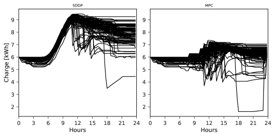
Figure 6: Hot water tank trajectories for SDDP (left) and MPC (right) during Summer day

This analysis suggests that SDDP makes a better use of storage capacities than MPC.

4.3 Quantifying the sensitivity of MPC and SDDP with respect to the level of uncertainty

Here, we compare the performances of the two algorithms (MPC and SDDP) when the level of uncertainty increases.

Uncertainty model

We suppose that, at each time step $t$, the random variable $\boldsymbol{\Phi}^{pv}_{t}$ (the photovoltaic production in Equation (1)) is given by $\boldsymbol{\Phi}^{pv}_{t}=\mu_{t}\times(1+\boldsymbol{\varepsilon^{\textstyle\text{\unboldmath$\scriptstyle$}}_{\textstyle\text{\unboldmath$\scriptstyle t$}}})$, where $\mu_{t}$ is deterministic (it corresponds to the forecasted value of $\boldsymbol{\Phi}^{pv}_{t}$) and where $\boldsymbol{\varepsilon^{\textstyle\text{\unboldmath$\scriptstyle$}}_{\textstyle\text{\unboldmath$\scriptstyle t$}}}$ is a zero-mean Gaussian random variable, with standard-deviation $\sigma_{t}=\sigma_{0}+(\sigma_{T}-\sigma_{0}){t}/{T}$ increasing linearly over time (where $\sigma_{0}$ is the initial standard-deviation and $\sigma_{T}$ the final standard-deviation). We define the level of uncertainty through the value of $\sigma_{T}$: the greater it is, the more difficult it becomes to predict the value of the random variable $\boldsymbol{\Phi}^{pv}_{t}$. With this setting, we have that $\mathbb{E}(\boldsymbol{\Phi}^{pv}_{t})=\mu_{t}$ and $\mathrm{Var}(\boldsymbol{\Phi}^{pv}_{t})=\mu_{t}^{2}\sigma_{t}^{2}$. In Figure 7, we display scenarios that are realizations of sequences $\boldsymbol{\Phi}^{pv}_{0},\ldots,\boldsymbol{\Phi}^{pv}_{T}$.

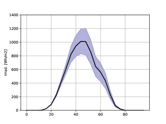
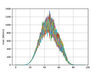
(a)	(b)

Figure 7: Confidence interval (a) and generation of corresponding assessment scenarios (b) for production of solar panel $\boldsymbol{\Phi}^{pv}$. These scenarios are generated with $\sigma_{0}=0$ and $\sigma_{T}=0.2$.

Results

We assess SDDP and MPC with different level of uncertainties, that is, with increasing values of $\sigma_{T}$. The costs correspond to the management costs to operate the microgrid during a particular day in Summer, where the production of the solar panel is nominal. The detailed results are given in Figure 8, which shows the evolution of the performance of the two algorithms as a function of the level $\sigma_{T}$ of uncertainty. The costs of each algorithm are obtained via Monte-Carlo simulation, with 10,000 assessment scenarios. We observe that MPC’s cost increases quicker than SDDP’s cost when the level of uncertainty increases.

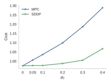
Figure 8: Evolution of the performance of MPC and SDDP as a function of the level $\sigma_{T}$ of uncertainty

This second use case allows to quantify the sensitivity of the algorithms with respect to the level of uncertainty. It seems that SDDP behaves better than MPC when facing high uncertainties.

5 Conclusion

We have presented the optimal management of a domestic microgrid, and have compared different management policies (the core of an Energy Management System) under uncertainties. Our results show that the two optimization-based policies (MPC and SDDP) outperform the proposed rule based policy in terms of money savings. Furthermore, SDDP outperforms MPC during Winter and Summer days — and displays similar performance as MPC during Spring day. Even when SDDP and MPC exhibit close average performances, a comparison scenario by scenario shows that SDDP beats MPC most of the time (more than 90% of scenarios during Summer day). Thus, SDDP proves better than MPC to manage uncertainties in our study, although MPC displays also good performances. SDDP makes better use of storage capacities too.

What if we had compared SDDP not only with “ordinary” MPC but with its stochastic variant, Stochastic Model Predictive Control (SMPC)? A systematic analysis done in [30], using a large dataset of microgrids, reveals that our conclusions remain valid: algorithms based on the offline computation of cost-to-go functions (SDP, SDDP) outperform lookahead algorithms (MPC, SMPC).

Our study can be extended in different directions. First, we could mix SDDP and MPC to grasp the benefits of these two algorithms. Indeed, SDDP is designed to handle the uncertainties variability but fails to capture the time correlation (as it relies on an assumption of stagewise independence), whereas ordinary MPC ignores the uncertainties variability, but considers time correlation by means of a future scenario. Second, we have extended this study in [31], where we applied decomposition methods to optimize microgrids comprising several buildings connected together. Finally, a comparison of MPC and SDDP with novel methods based on reinforcement learning could also be of interest.

6 Appendix

In this Appendix, we depict physical equations of the energy system in Figure 1. These equations are naturally written in continuous time $t$. We model the battery and the hot water tank with stock dynamics, and the dynamics of the house’s temperatures with an electrical analogy.

6.1 Energy storage

We consider a battery, whose state of charge at time $t$ is denoted by $b(t)$. The battery dynamics is given by the differential equation

$$\dfrac{db}{dt}=\rho_{c}(f^{b}(t))^{+}-\dfrac{1}{\rho_{d}}(f^{b}(t))^{-}\;,$$ (21)

with $\rho_{c}$ and $\rho_{d}$ being the charge and discharge efficiency and $f^{b}(t)$ denoting the energy exchange with the battery.

6.2 Electrical hot water tank

We use a simple linear model for the electrical hot water tank dynamics. The enthalpy balance equation writes

$$\dfrac{dh}{dt}=\beta_{h}f^{w}(t)-d^{th}(t)\;,$$ (22)

where

• $f^{h}(t)$ is the electrical energy used to heat the tank, satisfying

  $$0\leq f^{w}(t)\leq\overline{f}^{w}\;,$$ (23)

• $d^{th}(t)$ is the domestic hot water demand,

• $\beta_{h}$ is a conversion yield.

6.3 Thermal envelope

We model the evolution of the temperatures inside the house with an electrical analogy: we view temperatures as voltages, walls as capacitors, and thermal flows as currents. A model with 6 resistances and 2 capacitors (R6C2) proves to be accurate to describe small buildings [32]. The model takes into account two temperatures:

• the wall’s temperature $\theta^{w}(t)$,

• the inner temperature $\theta^{i}(t)$.

Their evolution is governed by the two following differential equations

$$c_{m}\dfrac{d\theta^{w}}{dt}=\underbrace{\dfrac{\theta^{i}(t)-\theta^{w}(t)}{R_{i}+R_{s}}}_{\begin{subarray}{c}\text{Exchange}\\ \text{ Indoor/Wall}\end{subarray}}+\underbrace{\dfrac{\theta^{e}(t)-\theta^{w}(t)}{R_{m}+R_{e}}}_{\begin{subarray}{c}\text{Exchange}\\ \text{ Outdoor/Wall}\end{subarray}}+\underbrace{\gamma f^{t}(t)}_{\text{Heater}}\\ +\underbrace{\dfrac{R_{i}}{R_{i}+R_{s}}\Phi^{int}(t)}_{\begin{subarray}{c}\text{Radiation}\\ \text{through windows}\end{subarray}}+\underbrace{\dfrac{R_{e}}{R_{e}+R_{m}}\Phi^{ext}(t)}_{\begin{subarray}{c}\text{Radiation}\\ \text{through wall}\end{subarray}}\;,$$ (24a)

$$c_{i}\dfrac{d\theta^{i}}{dt}=\underbrace{\dfrac{\theta^{w}(t)-\theta^{i}(t)}{R_{i}+R_{s}}}_{\begin{subarray}{c}\text{Exchange}\\ \text{ Indoor/Wall}\end{subarray}}+\underbrace{\dfrac{\theta^{e}(t)-\theta^{i}(t)}{R_{v}}}_{\text{Ventilation}}+\underbrace{\dfrac{\theta^{e}(t)-\theta^{i}(t)}{R_{f}}}_{\text{Windows}}\\ +\underbrace{(1-\gamma)f^{t}(t)}_{\text{Heater}}+\underbrace{\dfrac{R_{s}}{R_{i}+R_{s}}\Phi^{int}(t)}_{\begin{subarray}{c}\text{Radiation}\\ \text{through windows}\end{subarray}}\;,$$ (24b)

where we denote

• the energy injected in the heater by $f^{h}(t)$,

• the external temperature by $\theta^{e}(t)$,

• the radiation through the wall by $\Phi^{ext}(t)$,

• the radiation through the windows by $\Phi^{int}(t)$.

The time-varying quantities $\theta^{e}(t)$, $\Phi^{int}(t)$ and $\Phi^{ext}(t)$ are exogenous. We denote by $R_{i},R_{s},R_{m},R_{e},R_{v},R_{f}$ the different resistances of the R6C2 model, and by $c_{i},c_{m}$ the capacities of the inner rooms and the walls. We denote by $\gamma$ the proportion of heating dissipated in the wall through conduction, and by $(1-\gamma)$ the proportion of heating dissipated in the inner room through convection. We detail the numerical values in Table 4.

$R_{i}$	$4.81\times 10^{-4}$ SI
$R_{s}$	$2.94\times 10^{-4}$ SI
$R_{m}$	$4.51\times 10^{-3}$ SI
$R_{e}$	$1.48\times 10^{-4}$ SI
$R_{v}$	$4.51\times 10^{-3}$ SI
$R_{f}$	$2.00\times 10^{-2}$ SI
$c_{i}$	$8.30\times 10^{7}$  SI
$c_{m}$	$5.85\times 10^{6}$  SI

Table 4: Numerical values for the electrical analogy

6.4 MPC

Building offline an AR model for MPC

We fit an AR(1) model using the optimization scenarios (we do not consider higher order lags for the sake of simplicity). For $i\in\{el,hw\}$, the AR model writes

$$d^{i}_{t+1}=\alpha_{t}^{i}d^{i}_{t}+\beta_{t}^{i}+\varepsilon_{t}^{i}\;,$$ (25a)

where the nonstationary coefficients $$(\alpha^{i}_{t},\beta^{i}_{t}) t$$ are, for any time step , solutions of the least-square problem

$$(\alpha^{i}_{t},\beta_{t}^{i})=\mathop{\arg\min}_{a,b}\sum_{s=1}^{N_{opt}}\left\|d^{i,s}_{t+1}-ad^{i,s}_{t}-b\right\|^{2}_{2}\;.$$ (25b)

The points $$(d^{i,1}_{t},\ldots d_{t}^{i,N_{opt}}) (\varepsilon_{t}^{el},\varepsilon_{t}^{hw})$$ correspond to the optimization scenarios. The AR residuals are a white noise process.

Updating the forecast online

Once the AR model is calibrated, we use it to update the forecast during assessment (see §3.1). The update procedure is threefold:

• we observe the demands $w_{t}=(d^{el}_{t},d^{hw}_{t})$ between time steps $t-1$ and $t$,

• we update the forecast $\overline{w}_{t+1}$ at time step $t+1$ with the AR model

  $$\overline{w}_{t+1}=\big{(}\overline{d}^{el}_{t+1},\overline{d}^{hw}_{t+1}\big{)}=\Big{(}\alpha_{t}^{el}d^{el}_{t}+\beta_{t}^{el},\;\alpha_{t}^{hw}d^{hw}_{t}+\beta_{t}^{hw}\Big{)}\;,$$

• we set the forecast between time steps $t+2$ and $T$ by using the mean values

  $$\overline{w}_{\tau}=\dfrac{1}{N_{opt}}\sum_{i=1}^{N_{opt}}w_{\tau}^{i}\quad\forall\tau=t+2,\cdots,T$$

  of the optimization scenarios

Once the forecast $(\overline{w}_{t+1},\ldots,\overline{w}_{T})$ is available, it serves as input into the optimization Problem (15) (the MPC algorithm).

References

- [1] D. E. Olivares, A. Mehrizi-Sani, A. H. Etemadi, C. A. Cañizares, R. Iravani, M. Kazerani, A. H. Hajimiragha, O. Gomis-Bellmunt, M. Saeedifard, R. Palma-Behnke, G. A. Jiménez-Estévez, and N. D. Hatziargyriou, “Trends in microgrid control,” IEEE Transactions on Smart Grid, vol. 5, no. 4, pp. 1905–1919, 2014.
- [2] T. Morstyn, B. Hredzak, and V. G. Agelidis, “Control strategies for microgrids with distributed energy storage systems: An overview,” IEEE Transactions on Smart Grid, vol. 9, no. 4, pp. 3652–3666, 2016.
- [3] C. E. Garcia, D. M. Prett, and M. Morari, “Model predictive control: theory and practice—a survey,” Automatica, vol. 25, no. 3, pp. 335–348, 1989.
- [4] A. Mesbah, “Stochastic model predictive control: An overview and perspectives for future research,” IEEE Control Systems Magazine, vol. 36, no. 6, pp. 30–44, 2016.
- [5] J. Širokỳ, F. Oldewurtel, J. Cigler, and S. Prívara, “Experimental analysis of model predictive control for an energy efficient building heating system,” Applied energy, vol. 88, no. 9, pp. 3079–3087, 2011.
- [6] N. Holjevac, T. Capuder, and I. Kuzle, “Adaptive control for evaluation of flexibility benefits in microgrid systems,” Energy, vol. 92, pp. 487–504, 2015.
- [7] D. E. Olivares, J. D. Lara, C. A. Cañizares, and M. Kazerani, “Stochastic-predictive energy management system for isolated microgrids,” IEEE Transactions on Smart Grid, vol. 6, no. 6, pp. 2681–2693, 2015.
- [8] R. R. Appino, J. Á. G. Ordiano, R. Mikut, T. Faulwasser, and V. Hagenmeyer, “On the use of probabilistic forecasts in scheduling of renewable energy sources coupled to storages,” Applied energy, vol. 210, pp. 1207–1218, 2018.
- [9] K. Paridari, A. Parisio, H. Sandberg, and K. H. Johansson, “Robust scheduling of smart appliances in active apartments with user behavior uncertainty,” IEEE Transactions on Automation Science and Engineering, vol. 13, no. 1, pp. 247–259, 2016.
- [10] M. De Lara, P. Carpentier, J.-P. Chancelier, and V. Leclère, Optimization Methods for the Smart Grid. Conseil Francais de l’Energie, 2014.
- [11] M. V. Pereira and L. M. Pinto, “Multi-stage stochastic optimization applied to energy planning,” Mathematical programming, vol. 52, no. 1-3, pp. 359–375, 1991.
- [12] P. Haessig, H. B. Ahmed, and B. Multon, “Energy storage control with aging limitation,” in 2015 IEEE Eindhoven PowerTech, pp. 1–6, IEEE, 2015.
- [13] B. Heymann, J. F. Bonnans, F. Silva, and G. Jimenez, “A stochastic continuous time model for microgrid energy management,” in European Control Conference (ECC), pp. 2084–2089, IEEE, 2016.
- [14] C. Alasseur, A. Balata, S. B. Aziza, A. Maheshwari, P. Tankov, and X. Warin, “Regression Monte Carlo for microgrid management,” ESAIM: Proceedings and Surveys, vol. 65, pp. 46–67, 2019.
- [15] D. P. Bertsekas, Dynamic programming and optimal control, vol. 1. Athena Scientific Belmont, MA, third ed., 2005.
- [16] A. Shapiro, “Analysis of stochastic dual dynamic programming method,” European Journal of Operational Research, vol. 209, no. 1, pp. 63–72, 2011.
- [17] A. B. Philpott and Z. Guan, “On the convergence of stochastic dual dynamic programming and related methods,” Operations Research Letters, vol. 36, no. 4, pp. 450–455, 2008.
- [18] P. Girardeau, V. Leclère, and A. B. Philpott, “On the convergence of decomposition methods for multistage stochastic convex programs,” Mathematics of Operations Research, vol. 40, no. 1, pp. 130–145, 2014.
- [19] A. Bhattacharya, J. P. Kharoufeh, and B. Zeng, “Managing energy storage in microgrids: A multistage stochastic programming approach,” IEEE Transactions on Smart Grid, vol. 9, no. 1, pp. 483–496, 2018.
- [20] A. Papavasiliou, Y. Mou, L. Cambier, and D. Scieur, “Application of stochastic dual dynamic programming to the real-time dispatch of storage under renewable supply uncertainty,” IEEE Transactions on Sustainable Energy, vol. 9, no. 2, pp. 547–558, 2018.
- [21] A. Balata, M. Ludkovski, A. Maheshwari, and J. Palczewski, “Statistical learning for probability-constrained stochastic optimal control,” European Journal of Operational Research, vol. 290, no. 2, pp. 640–656, 2021.
- [22] O. Kallenberg, Foundations of Modern Probability. Springer-Verlag, New York, second ed., 2002.
- [23] R. Bellman, Dynamic Programming. New Jersey: Princeton University Press, 1957.
- [24] Journal Officiel de la République Française, Arrêté du 28 décembre 2012 relatif aux caractéristiques thermiques et aux exigences de performance énergétique des bâtiments nouveaux, 2013.
- [25] I. Dunning, J. Huchette, and M. Lubin, “JuMP: A modeling language for mathematical optimization,” SIAM Review, vol. 59, no. 2, pp. 295–320, 2017.
- [26] Gurobi Optimization Inc, “Gurobi Optimizer Reference Manual,” 2014.
- [27] R. Baetens and D. Saelens, “Modelling uncertainty in district energy simulations by stochastic residential occupant behaviour,” Journal of Building Performance Simulation, vol. 9, no. 4, pp. 431–447, 2016.
- [28] S. Lloyd, “Least squares quantization in PCM,” IEEE transactions on information theory, vol. 28, no. 2, pp. 129–137, 1982.
- [29] J. Widén and E. Wäckelgård, “A high-resolution stochastic model of domestic activity patterns and electricity demand,” Applied Energy, vol. 87, no. 6, pp. 1880–1892, 2010.
- [30] A. Le Franc, P. Carpentier, J.-P. Chancelier, and M. De Lara, “EMSx: A numerical benchmark for energy management systems,” Energy Systems, Feb. 2021.
- [31] P. Carpentier, J. P. Chancelier, M. De Lara, and F. Pacaud, “Mixed spatial and temporal decompositions for large-scale multistage stochastic optimization problems,” Journal of Optimization Theory and Applications, vol. 186, no. 3, pp. 985–1005, 2020.
- [32] T. Berthou, P. Stabat, R. Salvazet, and D. Marchio, “Development and validation of a gray box model to predict thermal behavior of occupied office buildings,” Energy and Buildings, vol. 74, pp. 91–100, 2014.