From Small Scales to Large Scales: Distance-to-Measure Density based Geometric Analysis of Complex Data

Abstract

How can we tell complex point clouds with different small scale characteristics apart, while disregarding global features? Can we find a suitable transformation of such data in a way that allows to discriminate between differences in this sense with statistical guarantees?

In this paper, we consider the analysis and classification of complex point clouds as they are obtained, e.g., via single molecule localization microscopy. We focus on the task of identifying differences between noisy point clouds based on small scale characteristics, while disregarding large scale information such as overall size. We propose an approach based on a transformation of the data via the so-called Distance-to-Measure (DTM) function, a transformation which is based on the average of nearest neighbor distances. For each data set, we estimate the probability density of average local distances of all data points and use the estimated densities for classification. While the applicability is immediate and the practical performance of the proposed methodology is very good, the theoretical study of the density estimators is quite challenging, as they are based on non-i.i.d. observations that have been obtained via a complicated transformation. In fact, the transformed data are stochastically dependent in a non-local way that is not captured by commonly considered dependence measures. Nonetheless, we show that the asymptotic behaviour of the density estimator is driven by a kernel density estimator of certain i.i.d. random variables by using theoretical properties of U-statistics, which allows to handle the dependencies via a Hoeffding decomposition. We show via a numerical study and in an application to simulated single molecule localization microscopy data of chromatin fibers that unsupervised classification tasks based on estimated DTM-densities achieve excellent separation results.

Keywords Geometric data analysis, Distance-to-Measure signature, kernel density estimators, nearest neighbor distributions

1 Introduction

The analysis and extraction of information from complex point clouds has become a main task in many applications. Prominent examples can be found in geomorphology, where structure in point-clouds obtained from laser scanners is investigated to infer on the shape of the Earth [54, 27], or in cosmology, where the Cosmic Web is analysed based on a discrete set of points from $N$-body simulations or galaxy studies [32]. Related questions also arise in biology, when data from single molecule localization microscopy (SMLM), which is based on the localization of fluorescent molecules that appear at different times, are analyzed [42, 31]. Data obtained in SMLM are 2D or 3D point clouds, where the points correspond to particular molecular localization events. In this paper, we consider a specific example which is related to the analysis of super-resolution visualization of human chromosomal regions as it has recently been investigated in Hao et al. [26]. In this application, the goal is to better understand the 3D organization of the chromatin fiber in cell nuclei, which plays a key role in the regulation of gene expression.
In all aforementioned examples, it is important to identify significant differences between noisy point clouds, where a focus is on general structure and small scale information rather than on global features such as the overall shape of a point cloud.

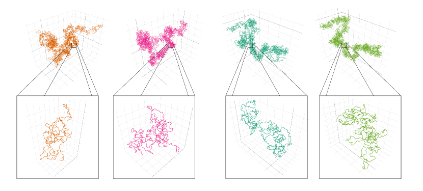
Figure 1: Example Data: Four different simulated chromatin fibers in two different conditions: Condition A (orange (far left) and blue-green (middle right)) and Condition B (pink (middle left) and green (far right)) for the purpose of comparison.

For illustration, Figure 1 shows four simulated chromatin fibers in two different conditions. The displayed structures form loops of different sizes and frequencies, based on the condition under which they were simulated, where the differences are very subtle. In the application considered in this paper, we analyse noisy samples of such simulated structures. The noise accounts for localization errors as they are present in real SMLM data. The loops are of sizes comparable to the resolution of the images (see Section 4 and Hao et al. [26] for more details), which makes the problem tractable but difficult. The aim is to classify the point clouds based on their loop distribution (i.e. based on their small scale characteristics), while disregarding their total size or large scale shapes. It is natural to transform such complicated data prior to the analysis, in particular when one has a clear objective in mind. In the above reference, the statistical analysis of the simulated and real data was based on a transformation of each data cloud onto a set of two parameters, capturing smoothness and local curvature of the point clouds. While this transformation provided a clear discrimination between different groups, the amount of information preserved in a two-dimensional parameter is not sufficient as a basis for point-by-point classification. In this paper, we propose an approach which is similar in spirit, but which provides a transformation into a curve, with different characteristics for the different conditions. In our analysis, the whole curves are then used as features. To this end, we perform the following two steps.

• A transformation of the data points in a point cloud based on the Distance-to-Measure (DTM) signature [13, 14] to a one-dimensional data set,

• The analysis of the distribution of the DTM-transformed data via their estimated probability density.

The DTM signature is closely related to certain nearest neighbor distributions, which makes this approach very intuitive. In particular, this framework allows for a comprehensive exploratory analysis of complex data, for which we might seek a simple graphical representation that captures and summarizes the local structural information well.

1.1 The DTM-Density as a Representation for Local Features

We now introduce the statistical framework of the paper and carefully define the previously mentioned DTM-signature. Throughout the following, we consider random point clouds as samples from a Euclidean metric measure space $\mathcal{X}=\left(\mathcal{X},||\cdot||,\mu_{\mathcal{X}}\right)$, i.e., a triple, where $\mathcal{X}\subset\mathbb{R}^{d}$ denotes a compact set, $||\cdot||$ stands for the Euclidean distance and $\mu_{\mathcal{X}}$ denotes a probability measure that is fully supported on the compact set $\mathcal{X}$. If, additionally, $\mu_{\mathcal{X}}$ has a Lipschitz continuous density with respect to the $d$-dimensional Lebesgue measure, then we call $\mathcal{X}$ a regular Euclidean metric measure space. For each metric measure space $\mathcal{X}$, we can define the corresponding Distance-to-Measure (DTM) function with mass parameter $m\in(0,1]$ for $x\in\mathbb{R}^{d}$ as

$$\mathrm{d}^{2}_{\mathcal{X},m}(x)=\frac{1}{m}\int_{0}^{m}\!F_{x}^{-1}(u)\,du,$$ (1)

where $F_{x}(t)=P(\left\lVert X-x\right\rVert^{2}\leq t)$, $X\sim\mu_{\mathcal{X}}$, and $F_{x}^{-1}$ denotes the corresponding quantile function. The DTM function, which is essential for the definition of the DTM-signature, is a population quantity that is generally unknown in practice and thus has to be estimated from the data. In order to do so, we replace the quantile function in the definition (1) by its empirical version as follows. Let $X_{1}\dots,X_{n}\overset{i.i.d.}{\sim}\mu_{\mathcal{X}}$ and denote the corresponding empirical measure by $\widehat{\mu}_{\mathcal{X}}$. We define for $t\geq 0$

$$\widehat{F}_{x,n}(t)=\frac{1}{n}\sum_{i=1}^{n}\mathds{1}_{\left\{||x-X_{i}||^{2}\leq t\right\}}$$ (2)

and denote by $\widehat{F}_{x,n}^{-1}$ the corresponding quantile function, giving rise to a plug-in estimator for the Distance-to-Measure function $\mathrm{d}^{2}_{\mathcal{X},m}(x)$:

$${\delta}^{2}_{\mathcal{X},m}(x)=\frac{1}{m}\int_{0}^{m}\!\widehat{F}_{x,n}^{-1}(u)\,du.$$ (3)

In the special case that $m=\frac{k}{n}$, it is possible to rewrite (3) as a nearest neighbor statistic as follows

$${\delta}^{2}_{\mathcal{X},m}(x)=\frac{1}{k}\sum_{X_{i}\in N_{k}(x)}||X_{i}-x||^{2},$$ (4)

where $N_{k}(x)$ is the set containing the $k$ nearest neighbors of $x$ among the data points $X_{1},\dots,X_{n}$.

As discussed previously, we require a good descriptor for the small scale behavior of our data. Hence, in a similar spirit as Brécheteau [7], we reduce the potentially complex Euclidean metric measure space to a one-dimensional probability distribution by considering the Distance-to-Measure (DTM) signature $\mathrm{d}^{2}_{\mathcal{X},m}(X)$, where $X\sim\mu_{\mathcal{X}}$. That is, the deterministic point $x\in\mathcal{X}$ is replaced by the random variable $X$. The distribution of $\mathrm{d}^{2}_{\mathcal{X},m}(X)$ captures the relative frequency of the mean of the distances of a random point in $\mathcal{X}$ to its “$m\cdot 100\%$ nearest neighbors”. We will empirically illustrate that the distribution of $\mathrm{d}^{2}_{\mathcal{X},m}(X)$ is a good descriptor for the small scale behavior of the considered data for small values of $m$ and verify that it is well-suited for chromatin loop analysis. Furthermore, it is easy to see that for $m=1$ the random quantity $\mathrm{d}^{2}_{\mathcal{X},1}(X)$ is closely related to the lower bound $\text{FLB}_{p}$ of the Gromov-Wasserstein distance defined in Mémoli [37] and is well suited for object discrimination with a focus on large scale characteristics. Although this case is not of interest in our specific data example, we include it in our analysis, since variants of $\mathrm{d}^{2}_{\mathcal{X},1}(X)$ have been proven very useful for pose invariant object discrimination [25, 22].

Since we propose to reduce (possibly complex) multi-dimensional metric measure spaces to a one-dimensional probability distribution, the next step is to visualize and investigate these distributions. It is well known that probability densities (if they exist) usually provide a useful visual insight into the probability distributions considered. In this regard, they are usually better suited than cumulative distribution functions (see, e.g., Chen and Pokojovy [15]). Therefore, we focus on the estimation of the density of $\mathrm{d}^{2}_{\mathcal{X},m}(X)$ in this paper. A natural estimator for the density of $\mathrm{d}^{2}_{\mathcal{X},m}(X)$, in the following denoted as DTM-density, in case of a known DTM-function, is given by

$$\widehat{f}_{\mathrm{d}^{2}_{\mathcal{X},m}}(y)=\frac{1}{nh}\sum_{i=1}^{n}K\left(\frac{\mathrm{d}^{2}_{\mathcal{X},m}(X_{i})-y}{h}\right).$$ (5)

However, since $\mu_{\mathcal{X}}$ is usually unknown, we cannot calculate $\mathrm{d}^{2}_{\mathcal{X},m}$ and consequently it is generally not feasible to estimate $f_{\mathrm{d}^{2}_{\mathcal{X},m}}$ via $\widehat{f}_{\mathrm{d}^{2}_{\mathcal{X},m}}$. Instead, we propose to replace $\mathrm{d}^{2}_{\mathcal{X},m}$ by its empirical version ${\delta}^{2}_{\mathcal{X},m}$ and estimate $f_{\mathrm{d}^{2}_{\mathcal{X},m}}$ based on the plug-in estimator

$$\widehat{f}_{{\delta}^{2}_{\mathcal{X},m}}(y)=\frac{1}{nh}\sum_{i=1}^{n}K\left(\frac{{\delta}^{2}_{\mathcal{X},m}(X_{i})-y}{h}\right).$$ (6)

It is important to note that, in contrast to $\widehat{f}_{\mathrm{d}^{2}_{\mathcal{X},m}}$, the plug-in estimator $\widehat{f}_{{\delta}^{2}_{\mathcal{X},m}}$ is based on the non-i.i.d. observations ${\delta}^{2}_{\mathcal{X},m}(X_{1}),\ldots,{\delta}^{2}_{\mathcal{X},m}(X_{n})$. In fact, for each $i\neq j$, ${\delta}^{2}_{\mathcal{X},m}(X_{i})$ and ${\delta}^{2}_{\mathcal{X},m}(X_{j})$ are stochastically dependent. The asymptotic behaviour of kernel density estimators under dependence has been studied extensively in the literature for various mixing and linear processes connected to weakly dependent time series [10, 45, 34, 35, 56]. In all these settings, results on asymptotic normality similar to the i.i.d. case can be derived. Related results for spatial processes can be found, e.g., in Hallin et al. [24]. For long-range dependent data, the asymptotic behaviour of kernel density estimators changes drastically. Here, the empirical density process (based on kernel estimators of the marginal densities) converges weakly to a tight limit (see Csorgo and Mielniczuk [16]). For the sequence ${\delta}^{2}_{\mathcal{X},m}(X_{1}),\ldots,{\delta}^{2}_{\mathcal{X},m}(X_{n})$, however, a structure as in the above examples (in space or time) is not given. For each $i\neq j$, ${\delta}^{2}_{\mathcal{X},m}(X_{i})$ and ${\delta}^{2}_{\mathcal{X},m}(X_{j})$ are stochastically dependent in a way that is not captured by the dependency models considered in the literature discussed above.

1.2 Main Results

The main theoretical contribution of the paper is the distributional limit of the kernel density estimator defined in (6). More precisely, we prove (cf. Theorem 2.12), given certain regularity conditions on $f_{\mathrm{d}^{2}_{\mathcal{X},m}}$, $\mathrm{d}^{2}_{\mathcal{X},m}(y)$ and $\mathcal{X}$, (see Condition 2.2 in Section 2.1) that for $n\to\infty$, $h=o\left(n^{-1/5}\right)$ and $nh\to\infty$

$$\sqrt{nh}\left(\widehat{f}_{{\delta}^{2}_{\mathcal{X},m}}(y)-f_{\mathrm{d}^{2}_{\mathcal{X},m}}(y)\right)\Rightarrow N\left(0,f_{\mathrm{d}^{2}_{\mathcal{X},m}}(y)\int\!K^{2}(u)\,du\right).$$ (7)

This means that, although the kernel density estimator $\widehat{f}_{{\delta}^{2}_{\mathcal{X},m}}$ is based on transformed, dependent random variables, asymptotically, it behaves precisely as the inaccessible kernel density estimator $\widehat{f}_{\mathrm{d}^{2}_{\mathcal{X},m}}$ based on independent random variables. This entails that many methods which are feasible for kernel density estimators based on i.i.d. data, can be applied in this much more complex setting as well, with the same asymptotic justification.

1.3 Application

Chromosomes, which consist of chromatin fibres, are essential parts of cell nuclei in human beings and carry the genetic information important for heredity transmission. It is known by now that there are small scale self-interacting genomic regions, so called topologically associating domains (TADs) which are often associated with loops in the chromatin fibers [43]. As an application, we consider chromatin loop analysis, one aspect of which is to study the presence or absence of loops in the chromatin (see Section 4).
The local loop structure is very well characterized by local nearest neighbor means as illustrated on the right of Figure 2 and hence we propose to use DTM-signatures for tackling this issue. Figure 2 shows the pipeline for the data transformation (left) and the resulting kernel density estimators ($m=1/250$, biweight kernel, bandwidth selection as in Section 4) for the four data sets shown in Figure 1 (right, same coloring). It shows that the kernel density estimators mainly differ between the different conditions and not between the corresponding chromatin fibers and that the differences between the conditions are clearly pronounced. This demonstrates that the transformation allows for a qualitative analysis of the data.

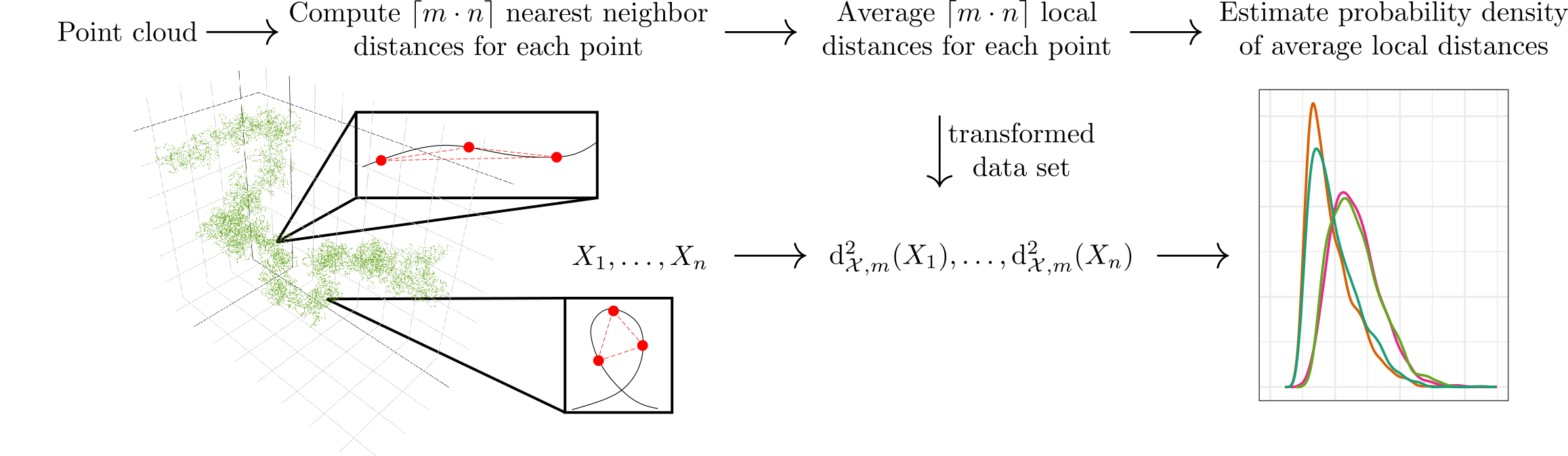
Figure 2: Data analysis pipeline: Illustration of the different steps in the proposed data analysis (left). The red dots in the details of the image represent data points, the red lines show the point-to-point distances, whereas the underlying chromatin structure is depicted by a black line. Right: The resulting DTM-density estimates of the point clouds illustrated in Figure 1 (same coloring).

1.4 Related Work

The use of the DTM-signature for the purpose of pose invariant object discrimination was proposed by Brécheteau [7], who in particular established a relation between the DTM-signature and the Gromov-Wasserstein distance (see Mémoli [37] for a definition). In the aforementioned work, the author considers the asymptotic behavior of the Wasserstein distance between sub-sampled estimates of the DTM-signatures for two different spaces. One big advantage of our method of estimating the DTM-densities over the former is that it does not require sub-sampling and all data points can be used for the analysis.
As illustrated in Section 1.1, the DTM-signature is based on the DTM-function (see (1)). This function has been thoroughly studied and applied in the context of support estimation and topological data analysis [11, 12, 9] and for its sample counterpart (see (3)) many consistency properties have been established in Chazal et al. [13, 14].

Distance based signatures for object discrimination have been applied and studied in a variety of settings [44, 21, 2, 47, 8, 3]. Recently, lower bounds of the Gromov-Wasserstein distance (see Mémoli [37]) have received some attention in applications [22] and in the investigation of their discriminating properties and their statistical behavior [38, 55].

Furthermore, it is noteworthy that nearest neighbor distributions are of great interest in various fields in biology [57, 39] as well as in physics [50, 4, 30]. In these fields it is quite common to consider the (mean of the) distribution of all nearest neighbors for data analysis. While this case corresponds to $m=1/n$ and is not included in our theoretic analysis, we would like to emphasize that taking the mean over a certain percentage of nearest neighbors makes our method a lot more robust against noise, which is why it performs so well in the analysis of noisy point clouds.
In the analysis of SMLM images, methods from spatial statistics are often employed. Related to the global distribution of all distances is Ripley’s K, which is used to infer on the amount and the degree of clustering in a given data set as compared to a point cloud generated by a homogeneous Poisson point process (see, e.g., Nicovich et al. [42] for the application of Ripley’s K in this context). Despite the connection via certain distributions of distances, the objectives and underlying models are quite different to the setting of this paper, such that a direct comparison is not straightforward.

Kernel density estimation from dependent data is a broad and well investigated topic. In addition to the references provided in Section 1.1, kernel density estimators of symmetric functions of the data and dyadic undirected data have been considered [20, 23]. In these settings, the summands of the corresponding kernel density estimators admit a “$U$-statistic like” dependency structure that has to be accounted for. While this is more closely related to the dependency structure which we are encountering in our analysis, the structure of the statistics that appear in the decomposition of the kernel density estimator (6) is quite different, such that those results cannot directly be transferred to our setting.

1.5 Organization of the Paper

In Section 2 we state the main results and are concerned with the derivation of (7) and the assumptions required for this.

Afterwards, in Section 3 we illustrate our findings via simulations. In Section 4, we apply our methodology to the classification within the framework of chromatin loop analysis.

Notation:

Throughout the following, we denote the $d$-dimensional Lebesgue measure by $\lambda^{d}$ and the $(d-1)$-dimensional surface measure in $\mathbb{R}^{d}$ by $\sigma^{d-1}$. We write $B(x,r)$ for the open ball in $\mathbb{R}^{d}$ (equipped with $||\cdot||$) with center $x$ and radius $r$. Given a function $f$ or a measure $\mu$, we write $\mathrm{supp}(f)$ and $\mathrm{supp}(\mu)$ to denote their respective support. Let $F$ be a distribution function with compact support $[a,b]$ and let $F^{-1}$ denote the corresponding quantile function. As frequently done, we set $F^{-1}(0)=a$ and $F^{-1}(1)=b$. Let $U\subseteq\mathbb{R}^{d_{1}}$ be an open set. We denote by $C^{k}(U,\mathbb{R}^{d_{2}})$ the set of all $k$-times continuously differentiable functions from $U$ to $\mathbb{R}^{d_{2}}$. Further, we denote by $C^{k,1}(U,\mathbb{R}^{d_{2}})$ the set of all $k$-times continuously differentiable functions from $U$ to $\mathbb{R}^{d_{2}}$, whose $k$’th derivative is Lipschitz continuous. For $d_{2}=1$, we abbreviate this to $C^{k}(U)$ and $C^{k,1}(U)$. If the domain and range of a function $g$ are clear from the context, we will usually write $g\in C^{k}$ or $g\in C^{k,1}$.

2 Distributional Limits

In this section, we state our main theoretical results, upon which our statistical methodology is based. We show that $\widehat{f}_{{\delta}^{2}_{\mathcal{X},m}}$ is a reasonable estimator for the density of the DTM-signature by proving the distributional limit (7). Before we come to this, we recall the setting, establish the conditions required and ensure that they are met in some simple examples.

2.1 Setting and Assumptions

First of all, we summarize the setting introduced in Section 1.1.

Setting 2.1.

Let $\left(\mathcal{X},||\cdot||,\mu_{\mathcal{X}}\right)$ denote a regular Euclidean metric measure space. For $x\in\mathcal{X}$ let $\mathrm{d}^{2}_{\mathcal{X},m}(x)$ denote the corresponding Distance-to-Measure function with mass parameter $m\in(0,1]$. Let $X\sim\mu_{\mathcal{X}}$ and assume that the Distance-to-Measure Signature $\mathrm{d}^{2}_{\mathcal{X},m}(X)$ has a density $f_{\mathrm{d}^{2}_{\mathcal{X},m}}$. Let $X_{1},\dots,X_{n}\overset{i.i.d.}{\sim}\mu_{\mathcal{X}}$ and denote by $\widehat{f}_{\mathrm{d}^{2}_{\mathcal{X},m}}$ and $\widehat{f}_{{\delta}^{2}_{\mathcal{X},m}}$ the kernel density estimators defined in (6) and (5), respectively.

It is noteworthy that the assumption that $\mathrm{d}^{2}_{\mathcal{X},m}(X)$ admits a Lebesgue density is slightly restrictive. The probability measure $\mu_{\mathrm{d}^{2}_{\mathcal{X},m}}$ of the DTM-signature can have a pure point component $\mu_{\mathrm{d}^{2}_{\mathcal{X},m},\text{pp}}$ in addition to the continuous component $\mu_{\mathrm{d}^{2}_{\mathcal{X},m},\text{cont}}$, if the spaces considered have very little local structure (for examples, see Section 2.2). That is,

$$\mu_{\mathrm{d}^{2}_{\mathcal{X},m}}=\mu_{\mathrm{d}^{2}_{\mathcal{X},m},\text{pp}}+\mu_{\mathrm{d}^{2}_{\mathcal{X},m},\text{cont}}.$$

If we define $f_{\mathrm{d}^{2}_{\mathcal{X},m}}$ to be the Radon-Nikodym derivative of the absolutely continuous component $\mu_{\mathrm{d}^{2}_{\mathcal{X},m},\text{cont}}$, i.e., $f_{\mathrm{d}^{2}_{\mathcal{X},m}}\mathrm{d}\lambda=\mathrm{d}\mu_{\mathrm{d}^{2}_{\mathcal{X},m},\text{cont}}$, the pointwise asymptotic analysis of $\widehat{f}_{{\delta}^{2}_{\mathcal{X},m}}$ performed in Section 2.3 (see Theorem 2.12) remains valid for all $y$ with $\mu_{\mathrm{d}^{2}_{\mathcal{X},m}}(\{y\})=0$ that meet the corresponding assumptions. This guarantees that our analysis remains meaningful even if parts of our space do not provide local structure that is discriminative.

In order to derive the statement (7), we require certain regularity assumptions on the density $f_{\mathrm{d}^{2}_{\mathcal{X},m}}$, the DTM function $\mathrm{d}^{2}_{\mathcal{X},m}$ and the kernel $K$. For the sake of completeness, we first recall some facts about the relation of the level sets of a given function. Let $g:\mathbb{R}^{d}\to\mathbb{R}$ and let $y\in\mathbb{R}$ be such that $g^{-1}(\{y\})\neq\emptyset$. Suppose that the function $g$ is continuously differentiable in an open environment of $g^{-1}(\{y\})$. Assume further that $\nabla g\neq 0$ on the level set $g^{-1}(\{y\})$. Then, it follows by Cauchy-Lipschitz’s theory that there exists a constant $h_{0}>0$, an open set $W\supset g^{-1}([y-h_{0},y+h_{0}])$ and a canonical one parameter family of $C^{1}$-diffeomorphisms $\Phi:[-h_{0},h_{0}]\times W\to\mathbb{R}^{d}$ with the following property:

$$\Phi(v,g^{-1}(\{y\}))=g^{-1}(\{y+v\})$$

for all $v\in[-h_{0},h_{0}]$ (for the precise construction of $\Phi$ see the proof of Lemma D.4 in Section D.1). Throughout the following, the family $\{\Phi(v,\cdot)\}_{v\in[-h_{0},h_{0}]}$ (also abbreviated to $\Phi$) is referred to as canonical level set flow of $g^{-1}(\{y\})$.

Condition 2.2.

Let $f_{\mathrm{d}^{2}_{\mathcal{X},m}}$ be supported on $[D_{1},D_{2}]$ and let $y\in[D_{1},D_{2}]$. Assume that there exists $\epsilon>0$ such that $f_{\mathrm{d}^{2}_{\mathcal{X},m}}$ is twice continuously differentiable on $(y-\epsilon,y+\epsilon)$. Further, suppose that the function $\mathrm{d}^{2}_{\mathcal{X},m}:\mathbb{R}^{d}\to\mathbb{R}$ is $C^{2,1}$ on an open neighborhood of the level set

$$\Gamma_{y}\coloneqq{\mathrm{d}^{2}_{\mathcal{X},m}}^{-1}(\{y\})=\{x\in\mathbb{R}^{d}:\mathrm{d}^{2}_{\mathcal{X},m}(x)=y\},$$

that $\nabla\mathrm{d}^{2}_{\mathcal{X},m}\neq 0$ on $\Gamma_{y}$ and that there exists $h_{0}>0$ such that for all $-h_{0}<v<h_{0}$

$$\mathcal{I}_{\mathcal{X}}(y;v):=\int_{\Gamma_{y}}\!\left|\mathds{1}_{\left\{x\in\mathcal{X}\right\}}-\mathds{1}_{\left\{\Phi(v,x)\in\mathcal{X}\right\}}\right|\,d\sigma^{d-1}(x)\leq C_{y}|v|,$$ (8)

where $\{\Phi(v,\cdot)\}_{v\in[-h_{0},h_{0}]}$ denotes the canonical level set flow of $\Gamma_{y}$ and $C_{y}$ denotes a finite constant that depends on $y$ and $\mathrm{d}^{2}_{\mathcal{X},m}$. Suppose that the kernel $K:\mathbb{R}\to\mathbb{R}_{+}$, is an even, twice continuously differentiable function with $\mathrm{supp}(K)=[-1,1]$. If $m<1$, we assume additionally that there are constants $\kappa>0$ and $1\leq b<5$ such that for $u\in(0,1)$ it holds

$$\omega_{\mathcal{X}}(u)\coloneqq\sup_{x\in\mathcal{X}}\sup_{t,t^{\prime}\in(0,1)^{2},|t-t^{\prime}|<u}\left|F_{x}^{-1}(t)-F_{x}^{-1}(t^{\prime})\right|\leq\kappa u^{1/b}.$$ (9)

The satisfiability of Condition 2.2 is an important issue that is difficult to address in general. Hence, in Section 2.2 we will verify that the requirements of Condition 2.2 are met in several simple examples. Nevertheless, in order to put Condition 2.2 into a broader perspective, we first gather some known regularity properties of $\mathrm{d}^{2}_{\mathcal{X},m}$ as well as $\{F_{x}^{-1}\}_{x\in\mathcal{X}}$ and discuss the technical requirement (8) afterwards.

2.1.1 Regularity of $\mathrm{d}^{2}_{\mathcal{X},m}$ and $\{F_{x}^{-1}\}_{x\in\mathcal{X}}$

We distinguish between the cases $m<1$ and $m=1$ for the presentation of known regularity results. For $m<1$, the smoothness of $\mathrm{d}^{2}_{\mathcal{X},m}$ has been investigated in Chazal et al. [11], where the authors derived the following results.

Lemma 2.3.

1. Let $\left(\mathcal{X},||\cdot||,\mu_{\mathcal{X}}\right)$ denote an Euclidean metric measure space. Then, the function $\mathrm{d}^{2}_{\mathcal{X},m}:\mathbb{R}^{d}\to\mathbb{R}$ is almost everywhere twice differentiable.

2. If $\mathcal{X}=\left(\mathcal{X},||\cdot||,\mu_{\mathcal{X}}\right)$ denotes a regular Euclidean metric measure space, then the function $\mathrm{d}^{2}_{\mathcal{X},m}:\mathbb{R}^{d}\to\mathbb{R}$ is differentiable with derivative

   $$\nabla\mathrm{d}^{2}_{\mathcal{X},m}(x)=\frac{2}{m}\int\![x-y]\,d\bar{\mu}_{x}(y),$$

   where $\bar{\mu}_{x}=\mu_{\mathcal{X}}|_{B(x,\gamma_{\mu_{\mathcal{X}},m}(x))}$ and $\gamma_{\mu_{\mathcal{X}},m}(x)=\inf\{r>0:\mu_{\mathcal{X}}\left(\bar{B}(x,r)\right)>m\}.$

Another important point for the case $m<1$ is the verification of inequality (9). This corresponds to bounding a uniform modulus of continuity for the family $\{F_{x}^{-1}\}_{x\in\mathcal{X}}$. An application of Lemma 3 in Chazal et al. [13] immediately yields the subsequent result.

Lemma 2.4.

Let $\left(\mathcal{X},||\cdot||,\mu_{\mathcal{X}}\right)$ be a regular Euclidean metric measure space. Suppose that there are constants $a,b>0$ such that for all $r>0$ and all $x\in\mathcal{X}$

$$\mu_{\mathcal{X}}(B(x,r))\geq 1\wedge ar^{b}.$$ (10)

Then, it holds that

$$\omega_{\mathcal{X}}(u)\leq 2\left(\frac{h}{a}\right)^{1/b}\mathrm{diam}\left(\mathcal{X}\right).$$

Remark 2.5.

Condition (10) is frequently assumed in the context of shape analysis. Measures that fulfill (10) are often called (a,b)-standard (see Cuevas [17], Fasy et al. [18], Chazal et al. [13] for a detailed discussion of (a,b)-standard measures). In particular, we observe that our assumption (9) is met, whenever $b<5$.

In the case $m=1$, it is important to observe that the DTM function admits the following specific form:

$$\mathrm{d}^{2}_{\mathcal{X},1}(x)=\int_{0}^{1}\!F_{x}^{-1}(u)\,du=\mathbb{E}\left[||X-x||^{2}\right],$$ (11)

where $X\sim\mu_{\mathcal{X}}$. This identity allows us to derive the following lemma.

Lemma 2.6.

Let $\mathcal{X}=\left(\mathcal{X},||\cdot||,\mu_{\mathcal{X}}\right)$ denote a regular Euclidean metric measure space and let $X\sim\mu_{\mathcal{X}}$. Then, it holds that:

1. The function $\mathrm{d}^{2}_{\mathcal{X},1}:\mathbb{R}^{d}\to\mathbb{R}$ is given as

   $$x=(x_{1},\dots,x_{d})\mapsto(x_{1}-c_{1})^{2}+(x_{2}-c_{2})^{2}+\dots+(x_{d}-c_{d})^{2}+\zeta,$$ (12)

   where $c=(c_{1},\dots,c_{d})^{T}=\mathbb{E}\left[X\right]$ and $\zeta$ denotes a finite constant that can be made explicit.

2. The function $\mathrm{d}^{2}_{\mathcal{X},1}:\mathbb{R}^{d}\to\mathbb{R}$ is three times continuously differentiable.

3. We have $\nabla\mathrm{d}^{2}_{\mathcal{X},1}(x)=0$ if and only if $x=\mathbb{E}\left[X\right]$.

4. Consider the representation of $\mathrm{d}^{2}_{\mathcal{X},1}$ in (12). Set $\Gamma_{y}={\mathrm{d}^{2}_{\mathcal{X},1}}^{-1}(\{y\})$ and suppose that $\left(y-\mathbb{E}\left[||X-\mathbb{E}\left[X\right]||^{2}\right]\right)>2h_{0}>0$. Then, the canonical level set flow $\{\Phi(v,\cdot)\}_{v\in[-h_{0},h_{0}]}$ of $\Gamma_{y}$ considered as function from $[-h_{0},h_{0}]\times{\mathrm{d}^{2}_{\mathcal{X},1}}^{-1}([y-h_{0},y+h_{0}])$ to $\mathbb{R}^{d}$ is for $x=(x_{1},\dots,x_{d})$ given as

   $$(v,x)\!\mapsto\!\!\left(\!\!(x_{1}-c_{1})\sqrt{1+\frac{v}{||x-c||^{2}}}+c_{1},\dots,(x_{d}-c_{d})\sqrt{1+\frac{v}{||x-c||^{2}}}+c_{d}\right)\!.$$ (13)

In order to increase the readability of this section, the proof of Lemma 2.6 is postponed to Section A in the Appendix.

2.1.2 Discussion of assumption (8) in Condition 2.2

To conclude this section, we consider the technical assumption (8). First of all, it is obvious (if $\mathrm{d}^{2}_{\mathcal{X},m}$ is nowhere constant) that the assumption only comes into play for $d\geq 2$. Furthermore, we observe that it is trivially fulfilled if there exists some $\epsilon>0$ such that $\Gamma_{y-\epsilon}\subset\mathcal{X}$, $\Gamma_{y}\subset\mathcal{X}$ and $\Gamma_{y+\epsilon}\subset\mathcal{X}$. Only if this is not the case, there might be points $y\in\mathcal{X}$ for which (8) is not satisfied. However, the assumption will typically be satisfied for all points of regularity of the density $f_{\mathrm{d}^{2}_{\mathcal{X},m}}$. To provide some intuition on this matter, we will consider the following example.

Example 2.7.

Let $\mathcal{X}=[0,1]^{2}$ and let $\mu_{\mathcal{X}}$ stand for the uniform distribution on $\mathcal{X}$. In this case, using relation (11), we obtain for $x=(x_{1},x_{2})\in\mathcal{X}$

$$\mathrm{d}^{2}_{\mathcal{X},1}(x)=\mathbb{E}\left[||X-x||^{2}\right]=\left(x_{1}-\frac{1}{2}\right)^{2}+\left(x_{2}-\frac{1}{2}\right)^{2}+\frac{1}{6}.$$

The corresponding DTM-density is supported on $[1/6,2/3]$ and it is smooth everywhere except for $y=5/12$, where $f_{\mathrm{d}^{2}_{\mathcal{X},m}}$ has a kink (detailed computations are provided in Section B.3 in the appendix). The level sets $\Gamma_{y}$ ($y\geq 1/6$), are concentric circles centered at $(1/2,1/2)$ with radii $\sqrt{y-1/6}$. For all $y<5/12$ the level sets are fully contained in the open cube $(0,1)^{2}$. For all $y>5/12$, we have $\mathbb{R}^{2}\backslash[0,1]^{2}\cap\Gamma_{y}\neq\emptyset$, i.e., the level sets are at least partly outside of the cube $[0,1]^{2}$. This means that $y=5/12$ is, in a sense, a transition point. In order to check (8) for $y\geq 5/12$, we observe that Lemma 2.6 implies that for $v>0$, $y\in[5/12,2/3]$ and each $x\in\mathcal{X}$ the equality $\mathds{1}_{\left\{x\in\Gamma_{y}\cap\mathcal{X}\right\}}=0$ implies $\mathds{1}_{\left\{\Phi(v,x))\Gamma_{y}\cap\mathcal{X}\right\}}=0$, where $\Phi$ denotes the canonical level set flow of $\Gamma_{y}$. Consequently, it follows that

$$\mathcal{I}_{\mathcal{X}}(y;v)=\left|\int_{\Gamma_{y}}\!\mathds{1}_{\left\{x\in\mathcal{X}\right\}}-\mathds{1}_{\left\{\Phi(v,x)\in\mathcal{X}\right\}}\,d\sigma^{1}(x)\right|=\left|\mathcal{L}(\Gamma_{y}\cap\mathcal{X})-\mathcal{L}(\Gamma_{y+v}\cap\mathcal{X})\right|,$$

where $\mathcal{L}(\Gamma_{y}\cap\mathcal{X})$ stands for the length of the curve $\Gamma_{y}$ in $\mathcal{X}$ and $\mathcal{L}(\Gamma_{y+v}\cap\mathcal{X})$ is defined analogously. Using the above equality, it is easy to verify that the requirement (8) is satisfied for all $y\in[1/6,2/3]\backslash\{5/12\}.$ Figure 3 exemplarily illustrates the behavior of the level sets in a neighborhood of $(1/2,1)$. The figure shows the level sets $\Gamma_{5/12}$ in blue and $\Gamma_{5/12+v}$ for some $v>0$ as dotted line in black. We observe that for $0\leq v\leq h_{0}$ for some $h_{0}$ sufficiently small, the value of the integral $\mathcal{I}_{\mathcal{X}}(y;v)$ corresponds to $2\pi v$ minus four times the length of the red line, which can be calculated explicitly using a well-known formula for circular segments:

$$\mathcal{I}_{\mathcal{X}}(y;v)=\left|2\pi v-4\arcsin\left({2\sqrt{v-v^{2}}}\right)\right|\geq\sqrt{v}.$$

This proves that for $y=5/12$ the requirement (8) is not fulfilled.

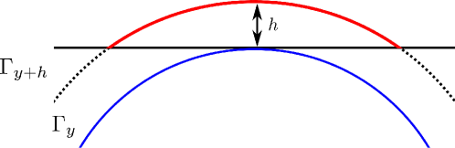
Figure 3: Tangential Level Set: Illustration of the behavior of the levels sets in a neighborhood of tangential intersection point with the boundary of $\mathcal{X}$ in the setting of Example 2.7.

We conclude this subsection by noting that the dimension of $\mathcal{X}$ heavily influences the regularity of (8). While it seems to be problematic, if $\Gamma_{y}$ intersects tangentially with the boundary $\partial\mathcal{X}$ of $\mathcal{X}$ for $d=2$, this is not necessarily the case for $d\geq 3$. In particular, if we consider $\mathcal{X}=[0,1]^{3}$ equipped with the uniform distribution, we find that for $y=3/4$ the level set $\Gamma_{y}$ tangentially touches $\partial\mathcal{X}$ at 6 points. However, here, it does not cause any problems. Following our considerations from Example 2.7, one can show that condition (8) holds for all points $y$ in the support of $f_{\mathrm{d}^{2}_{\mathcal{X},m}}$.

2.2 Examples of DTM-Densities

In the following, we will derive $\mathrm{d}^{2}_{\mathcal{X},m}$ as well as $f_{\mathrm{d}^{2}_{\mathcal{X},m}}$ in several simple examples explicitly and verify that in these settings Condition 2.2 is met almost everywhere. Since calculating $\mathrm{d}^{2}_{\mathcal{X},m}$ and $f_{\mathrm{d}^{2}_{\mathcal{X},m}}$ explicitly is quite cumbersome (especially for $m<1$), we concentrate on one- or two-dimensional examples. In order to increase the readability of this section, we postpone the the explicit, but lengthy representations of the derived DTM-functions and densities (as well as their derivation) to Section B.

We begin our considerations with the simplest case possible, the interval $[0,1]$ equipped with the uniform distribution.

Example 2.8.

Let $\mathcal{X}=[0,1]$ and let $\mu_{\mathcal{X}}$ denote the uniform distribution on $\mathcal{X}$. Furthermore, we consider two values for $m$, namely $m_{1}=1$ and $m_{2}=0.1$. In Section B.1, we derive $\mathrm{d}^{2}_{\mathcal{X},1}$, $\mathrm{d}^{2}_{\mathcal{X},0.1}$, $f_{\mathrm{d}^{2}_{\mathcal{X},1}}$ (see Figure 4 for an illustration). For $m=1$, the requirement (8) does not come into play as $\mathcal{X}$ is one-dimensional and $\mathrm{d}^{2}_{\mathcal{X},1}$ nowhere constant. Further, we point out that the density $f_{\mathrm{d}^{2}_{\mathcal{X},1}}$ is unbounded (however twice continuously differentiable on the interior of its support). In the case $m=0.1$ things are quite different. The function $\mathrm{d}^{2}_{\mathcal{X},0.1}$ is constant on $[0.05,0.95]$ and hence the random variable $\mathrm{d}^{2}_{\mathcal{X},0.1}(X)$, $X\sim\mu_{\mathcal{X}}$, does not have a Lebesgue density.

It is immediately clear that the DTM-signature can only admit a density with respect to the Lebesgue measure, if the DTM-function defined in (1) is almost nowhere constant. In Example 2.8 this is the case for $m_{1}=1$ but not for $m_{2}=0.1$. Recall that the DTM-function considers the quantile function of the random variable $||X-x||^{2}$, $\mathcal{X}\sim\mu_{\mathcal{X}}$, on $[0,m]$ for each $x\in\mathcal{X}$. In Example 2.8, $\mu_{\mathcal{X}}$ denotes the uniform measure on $\mathcal{X}=[0,1]$. Hence, it is evident in this setting that the quantile functions of the random variables $\{||X-x||\}_{x\in[m/2,1-m/2]}$ agree on $[0,m]$. Consequently, the corresponding DTM-signature admits a Lebesgue density only for $m=1$. In the next example, we equip $\mathcal{X}$ with another distribution, whose density is not constant on $\mathcal{X}$. In this case, we will find that also for $m<1$ the corresponding DTM-signature admits a Lebesgue density.

Example 2.9.

Let $\mathcal{X}=[0,1]$ and let $\mu_{\mathcal{X}}$ denote the probability distribution on $[0,1]$ with density $f(x)=2x$. Let $m=0.1$. In Section B.2, we derive $\mathrm{d}^{2}_{\mathcal{X},0.1}$ explicitly and demonstrate that the random variable $\mathrm{d}^{2}_{\mathcal{X},0.1}(X)$, $X\sim\mu_{\mathcal{X}}$, admits a Lebesgue density in this setting (see Figure 4 for an illustration). We observe that $\mathrm{d}^{2}_{\mathcal{X},0.1}$ is continuously differentiable everywhere and three times continuously differentiable almost everywhere. Further, the density $f_{\mathrm{d}^{2}_{\mathcal{X},0.1}}$ admits one discontinuity for $y=\frac{-683}{60}+18\sqrt{\frac{2}{5}}$ and is $C^{2}$ almost everywhere.

We observe that the DTM-densities derived in Example 2.8 and Example 2.9 are both unbounded. This has a simple explanation. Let $\left(\mathcal{X},||\cdot||,\mu_{\mathcal{X}}\right)$ be a regular Euclidean metric measure space and denote the $d$-dimensional Lebesgue density of $\mu_{\mathcal{X}}$ by $g_{\mu_{\mathcal{X}}}$. Suppose that $f_{\mathrm{d}^{2}_{\mathcal{X},m}}$ exists. Then, one can show (see e.g. Appendix C of Weitkamp et al. [55]) that

$$f_{\mathrm{d}^{2}_{\mathcal{X},m}}(y)=\int_{\left\{x\in\mathcal{X}:\mathrm{d}^{2}_{\mathcal{X},m}(x)=y\right\}}\frac{g_{\mu_{\mathcal{X}}}(u)}{||\nabla\mathrm{d}^{2}_{\mathcal{X},m}(u)||}\,d\sigma^{d-1}(u).$$ (14)

Since $d\sigma^{0}$ corresponds to integration with respect to the counting measure, the DTM-density of a one-dimensional Euclidean metric measure space is unbounded if there are $u\in\mathcal{X}$ with $|\nabla\mathrm{d}^{2}_{\mathcal{X},m}(u)|=0$ (this is the case in Example 2.8 and Example 2.9). However, it is important to note that this behavior mainly occurs for one-dimensional Euclidean metric measure spaces. For higher dimensional spaces, the area (w.r.t. $d\sigma^{d-1}$) of the set $A=\{x\in\mathcal{X}:||\nabla\mathrm{d}^{2}_{\mathcal{X},m}(u)||=0\}$, is usually a null set. Hence, it is possible that the density $f_{\mathrm{d}^{2}_{\mathcal{X},m}}$ defined in (14) remains bounded even if $A$ is non-empty (see Example 2.7 and Example 2.10).

To conclude this section and in order to illustrate that the showcased regularity of the DTM-function $\mathrm{d}^{2}_{\mathcal{X},m}$ and the DTM-density $f_{\mathrm{d}^{2}_{\mathcal{X},m}}$ does not only hold for one-dimensional settings, we consider two simple examples in $\mathbb{R}^{2}$ next. As the derivation of the family $(F_{x}^{-1})_{x\in\mathcal{X}}$ can be incredibly time consuming, we restrict ourselves in the following to the case $m=1$.

Example 2.7 (Continued).

Recall that $\mathcal{X}=[0,1]^{2}$, $\mu_{\mathcal{X}}$ stands for the uniform distribution on $\mathcal{X}$ and that $m=1$. Based on our previous considerations it is possible to derive $f_{\mathrm{d}^{2}_{\mathcal{X},1}}$ explicitly (see Section B.3 for the derivation). As illustrated in Figure 4, the density $f_{\mathrm{d}^{2}_{\mathcal{X},1}}$ is continuous. Moreover, it is twice continuously differentiable inside its support for $y\neq\frac{5}{12}$, which is also the only point where the requirements of (8) are not met, as discussed previously.

We note that the density $f_{\mathrm{d}^{2}_{\mathcal{X},1}}$ derived in Example 2.7 is constant on $[1/6,5/12]$. This kind of behavior is also expressed when considering a disc in $\mathbb{R}^{2}$ equipped with the uniform distribution (it is easy to verify that $f_{\mathrm{d}^{2}_{\mathcal{X},1}}$ is a constant function in this case). It is well known that it is difficult for kernel density estimators to approximate constant pieces or a constant function. However, it is not reasonable to assume that the data stems from a uniform distribution over a compact set in many applications (such as chromatin loop analysis). More often, it is possible to assume that the data generating distribution is more concentrated in the center of the considered set. The final example of this section showcases that in such a case the corresponding DTM-signature admits a density without any constant parts even on the disk.

Example 2.10.

Let $\mathcal{X}$ denote a disk in $\mathbb{R}^{2}$ centered at $(0,0)$ with radius 1 and let $\mu_{\mathcal{X}}$ denote probability measure with density

$$f(x_{1},x_{2})=\begin{cases}-\frac{2}{\pi}\left(x_{1}^{2}+x_{2}^{2}-1\right)&x_{1}^{2}+x_{2}^{2}\leq 1,\\ 0&\,\text{else.}\end{cases}$$

In this framework, we derive $\mathrm{d}^{2}_{\mathcal{X},1}$ and $f_{\mathrm{d}^{2}_{\mathcal{X},1}}$ in Section B.4. We observe that the level sets $\Gamma_{y}$ (of $\mathrm{d}^{2}_{\mathcal{X},1}$) are contained in $\mathcal{X}$ for any $y\in[1/3,4/3]$, i.e., condition (8) is met for all $y\in(1/3,4/3)$ in this setting. Further, we realize that $f_{\mathrm{d}^{2}_{\mathcal{X},1}}$ (see Figure 4 for an illustration) is smooth and nowhere constant on the interior of its support.

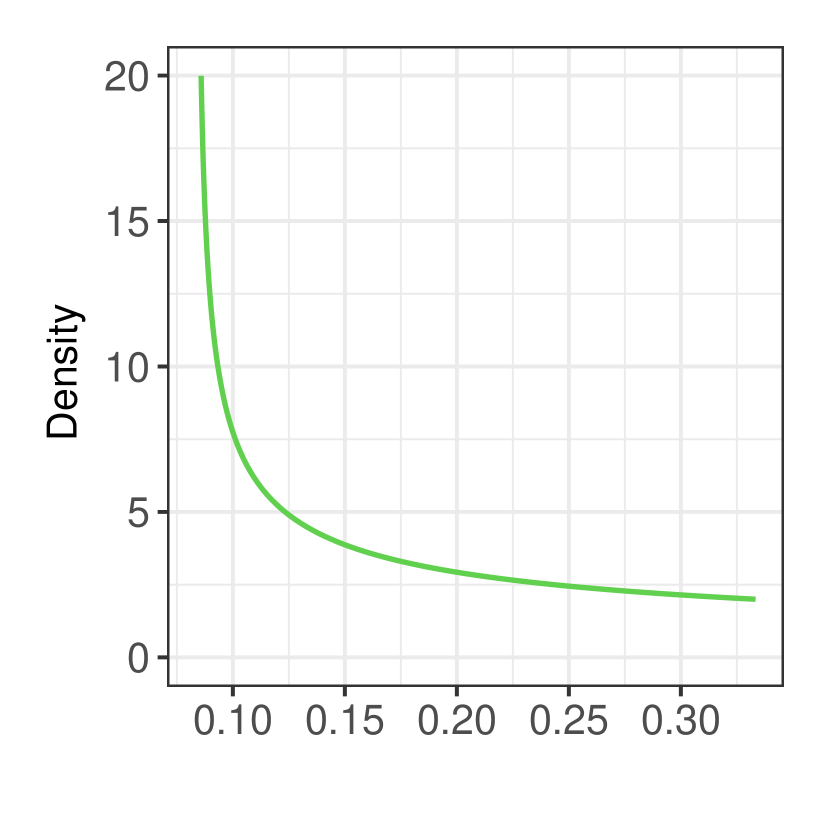
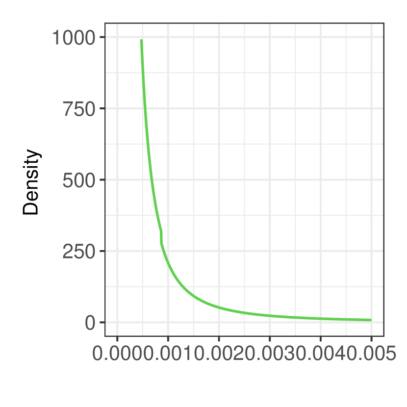
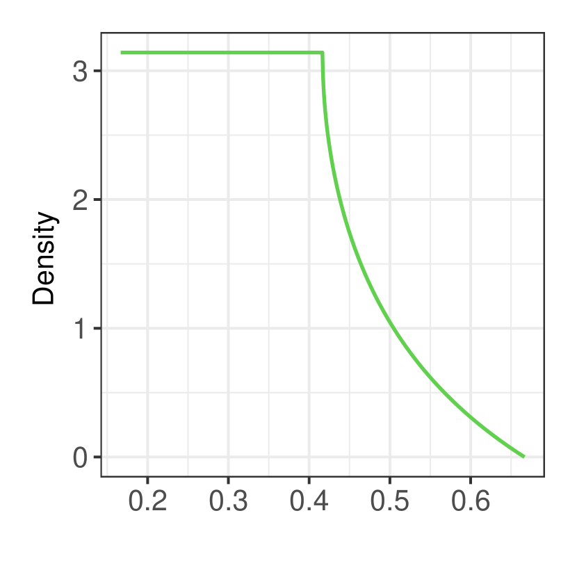
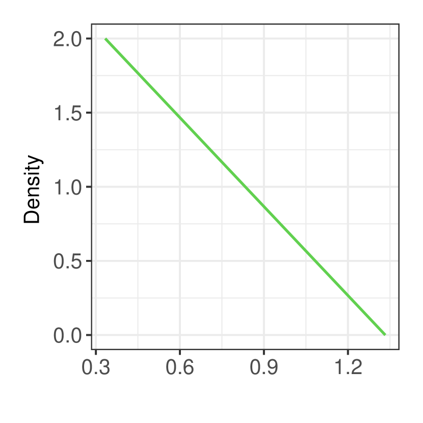
Figure 4: Distance-to-Measure signature: Illustration of the densities calculated in Example 2.8-2.9, Example 2.7 and Example 2.10 (from left to right).

2.3 Theoretical Results

In this section we study the asymptotic behavior of the kernel estimator of the DTM-density (6). Clearly, standard methodology implies the following pointwise central limit theorem for the kernel estimator $\widehat{f}_{\mathrm{d}^{2}_{\mathcal{X},m}}$ defined in (5).

Theorem 2.11.

Assume Setting 2.1 and suppose that $\mathrm{d}^{2}_{\mathcal{X},m}(X_{1})$ admits a density that is twice continuously differentiable in an environment of $y$. Suppose further that the kernel $K:\mathbb{R}\to\mathbb{R}_{+}$, is an even, twice continuously differentiable function with $\mathrm{supp}(K)=[-1,1]$. Then, it holds for $n\to\infty$, $h=o\left(n^{-1/5}\right)$ and $nh\to\infty$ that

$$\sqrt{nh}\left(\widehat{f}_{\mathrm{d}^{2}_{\mathcal{X},m}}(y)-f_{\mathrm{d}^{2}_{\mathcal{X},m}}(y)\right)\Rightarrow N\left(0,f_{\mathrm{d}^{2}_{\mathcal{X},m}}(y)\int\!K^{2}(u)\,du\right).$$

Surprisingly perhaps, despite the complicated stochastic dependence of the random variables ${\delta}^{2}_{\mathcal{X},m}(X_{i})$, asymptotically, $\widehat{f}_{\mathrm{d}^{2}_{\mathcal{X},m}}$ and $\widehat{f}_{{\delta}^{2}_{\mathcal{X},m}}$ behave equivalently in the following sense.

Theorem 2.12.

Assume Setting 2.1 and let Condition 2.2 hold. Then, it holds for $n\to\infty$, $h=o\left(n^{-1/5}\right)$ and $nh\to\infty$ that

$$\sqrt{nh}\left(\widehat{f}_{{\delta}^{2}_{\mathcal{X},m}}(y)-f_{\mathrm{d}^{2}_{\mathcal{X},m}}(y)\right)\Rightarrow N\left(0,f_{\mathrm{d}^{2}_{\mathcal{X},m}}(y)\int\!K^{2}(u)\,du\right).$$

As the the proof of Theorem 2.12 is lengthy and quite technical, it has been deferred to Appendix C. There, we will write the density estimator $\widehat{f}_{{\delta}^{2}_{\mathcal{X},m}}$ as a U-statistic plus remainder terms. Then, using a Hoeffding decomposition, the dependencies can be handled. However, showing that the remainder terms vanish is not trivial and requires the application of some tools from geometric measure theory.

3 Simulations

In the following, we investigate the finite sample behavior of $\widehat{f}_{{\delta}^{2}_{\mathcal{X},m}}$ in Monte Carlo simulations. To this end, we illustrate the pointwise limit derived in Theorem 2.11 in the setting of Example 2.10 and exemplarily highlight the discriminating potential of $\widehat{f}_{{\delta}^{2}_{\mathcal{X},m}}$. All simulations were performed in $\mathsf{R}$ ($\mathsf{R}$ Core Team [36]).

3.1 Pointwise Limit

We start with the illustration of Theorem 2.11. To this end, we consider the Euclidean metric measure space $\left(\mathcal{X},||\cdot||,\mu_{\mathcal{X}}\right)$ from Example 2.10. Recall that in this setting, $\mathcal{X}$ denotes a disk in $\mathbb{R}^{2}$ centered at $(0,0)$ with radius $1$ and that $\mu_{\mathcal{X}}$ denotes the probability measure with density

$$f(x_{1},x_{2})=\begin{cases}-\frac{2}{\pi}\left(x_{1}^{2}+x_{2}^{2}-1\right)&x_{1}^{2}+x_{2}^{2}\leq 1,\\ 0&\,\text{else.}\end{cases}$$

Now, we choose $m=1$ and consider

$$\widehat{f}_{{\delta}^{2}_{\mathcal{X},1}}(y)=\frac{1}{nh_{1}}\sum_{i=1}^{n}K_{Bi}\left(\frac{{\delta}^{2}_{\mathcal{X},m}(X_{i})-y}{h_{1}}\right),$$

where $K_{Bi}$ denotes the Biweight kernel, i.e.,

$$K_{Bi}(u)=\begin{cases}\frac{15}{16}\left(1-u^{2}\right)^{2}&|u|\leq 1,\\ 0&\,\text{else.}\end{cases}$$ (15)

Since we have calculated $\mathrm{d}^{2}_{\mathcal{X},1}$ explicitly (see (18)), it is of interest to compare the behavior of $\widehat{f}_{{\delta}^{2}_{\mathcal{X},1}}(y)$ to the one of

$$\widehat{f}_{\mathrm{d}^{2}_{\mathcal{X},1}}(y)=\frac{1}{nh_{2}}\sum_{i=1}^{n}K_{Bi}\left(\frac{\mathrm{d}^{2}_{\mathcal{X},1}(X_{i})-y}{h_{2}}\right).$$

As discussed previously, $\widehat{f}_{\mathrm{d}^{2}_{\mathcal{X},1}}$ is different from $\widehat{f}_{{\delta}^{2}_{\mathcal{X},1}}$ a kernel density estimator based on independent data, whose limit behavior is well understood (see Theorem 2.11). Nevertheless, for $y\in(1/3,4/3)$, $\widehat{f}_{\mathrm{d}^{2}_{\mathcal{X},1}}(y)$ and $\widehat{f}_{{\delta}^{2}_{\mathcal{X},1}}(y)$ admit the same asymptotic behavior according to Theorem 2.12, whose requirements can be easily checked in this setting (see Example 2.10). In order to illustrate this, we generate two independent samples $\{X_{i}\}_{i=1}^{n}$ and $\{X^{\prime}_{i}\}_{i=1}^{n}$ of $\mu_{\mathcal{X}}$ and calculate $\Delta_{n}=\{{\delta}^{2}_{\mathcal{X},1}(X_{i})\}_{i=1}^{n}$ as well as $D_{n}=\{\mathrm{d}^{2}_{\mathcal{X},1}(X_{i})\}_{i=1}^{n}$ for $n=50,500,2500,5000$. We set

$$h_{1}=(1.06\min\{s(\Delta_{n}),\text{IQR}(\Delta_{n})/1.34)\})^{5/4}n^{-1/4}$$

and

$$h_{2}=(1.06\min\{s(D_{n}),\text{IQR}(D_{n})/1.34)\})^{5/4}n^{-1/4},$$

where $s$ is the usual sample standard deviation and IQR denotes the inter quartile range. Based on $\Delta_{n}$ and $D_{n}$, we choose a central value of $y$ and calculate

$$\sqrt{nh_{1}}(\widehat{f}_{{\delta}^{2}_{\mathcal{X},1}}(y)-f_{\mathrm{d}^{2}_{\mathcal{X},1}}(y))\text{ and }\sqrt{nh_{2}}(\widehat{f}_{\mathrm{d}^{2}_{\mathcal{X},1}}(y)-f_{\mathrm{d}^{2}_{\mathcal{X},1}}(y)).$$ (16)

For each $n$, we repeat this process 5,000 times. The finite sample distributions of the quantities defined in (16) are compared to their theoretical normal counter part in Figure 5 (exemplarily for the specific choice of $y=0.7$). The kernel density estimators displayed (Gaussian kernel with bandwidth given by Silverman’s rule) highlight that the asymptotic behavior of $\widehat{f}_{{\delta}^{2}_{\mathcal{X},1}}(y)$ (red) matches that of $\widehat{f}_{\mathrm{d}^{2}_{\mathcal{X},1}}(y)$ (green). Further, we observe that even for small samples sizes both finite sample distributions strongly resemble their theoretical normal limit distribution (blue).

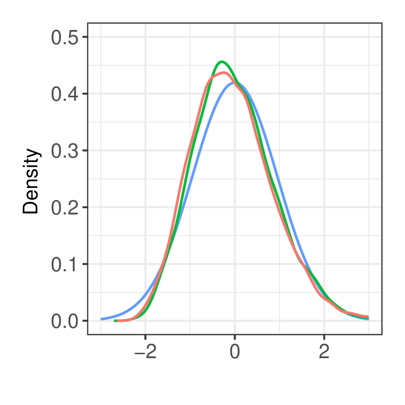
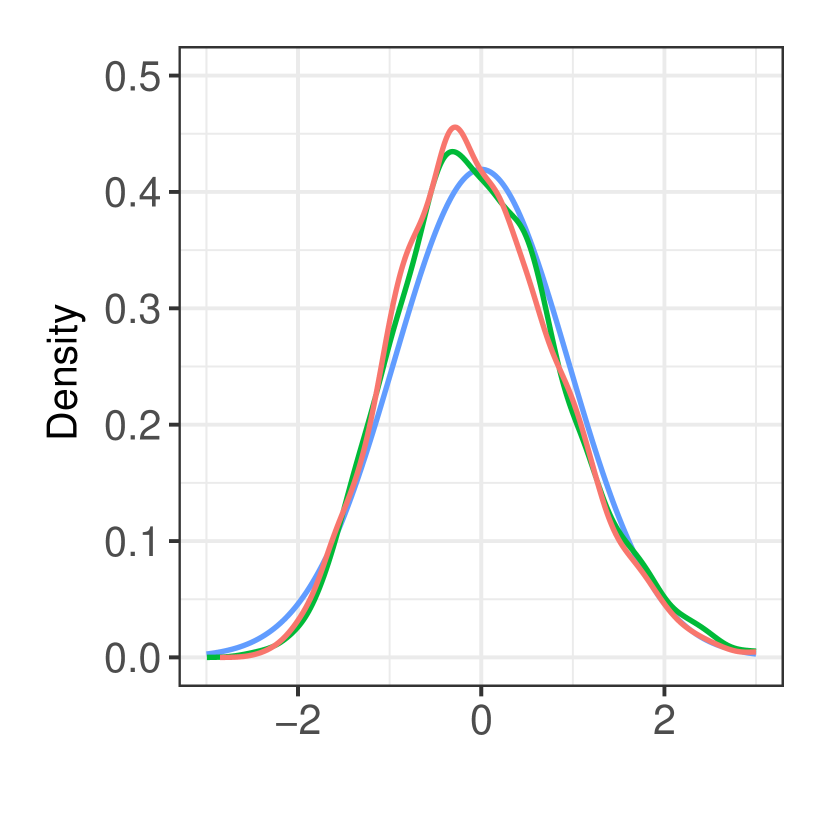
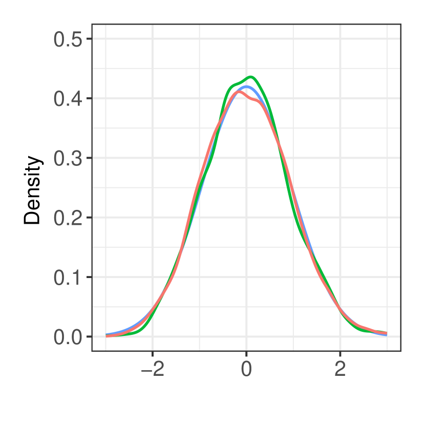
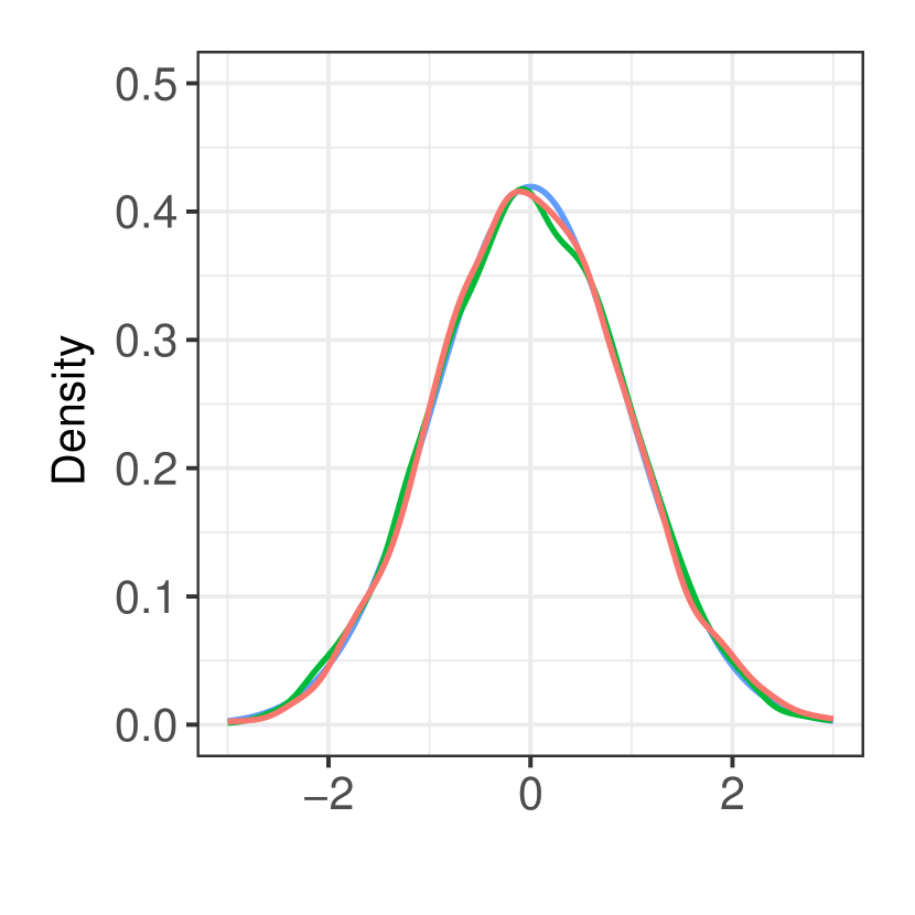
Figure 5: Pointwise limit distribution: Kernel density estimators of $\sqrt{nh_{1}}(\widehat{f}_{{\delta}^{2}_{\mathcal{X},1}}(0.7)-f_{\mathrm{d}^{2}_{\mathcal{X},1}}(0.7))$ (in red) and $\sqrt{nh_{2}}(\widehat{f}_{\mathrm{d}^{2}_{\mathcal{X},1}}(0.7)-f_{\mathrm{d}^{2}_{\mathcal{X},1}}(0.7))$ (in green) for $n=50,500,2500,5000$ (from left to right, sample size 5,000) and the normal limiting density (blue).

3.2 Discriminating Properties

In the remainder of this section, we will showcase empirically the potential of the DTM-signature for discriminating between different Euclidean metric measure spaces. To this end, let $\mu_{\mathcal{Y}_{1}}$ stand for the uniform distribution on a 3D-pentagon (inner pentagon side length: 1, Euclidean distance between inner and outer pentagon: 0.4, height: 0.4) and let $\mu_{\mathcal{Y}_{7}}$ denote the uniform distribution on a torus (center radius: 1.169, tube radius: 0.2) with the same center and orientation (see the plots for $t_{1}=0$ and $t_{7}=1$ in Figure 6). In order to interpolate between these measures, let $\Pi_{\mu_{\mathcal{Y}_{1}}}^{\mu_{\mathcal{Y}_{7}}}(t)$, $t\in[0,1]$, denote the 2-Wasserstein geodesic between $\mu_{\mathcal{Y}_{1}}$ and $\mu_{\mathcal{Y}_{7}}$ (see e.g. Santambrogio [46, Sec. 5.4] for a formal definition). Figure 6 displays the Euclidean metric measure spaces $\mathcal{Y}_{i}$, $1\leq i\leq 7$, corresponding to $\mu_{\mathcal{Y}_{i}}=\Pi_{\mu_{\mathcal{Y}_{1}}}^{\mu_{\mathcal{Y}_{7}}}(t_{i})$ for $t_{i}\in\{0,0.1,0.2,0.4,0.6,0.8,1\}$ (the geodesic has been approximated discretely based on 40,000 points with the the $\mathsf{WSGeometry}$-package [28]).

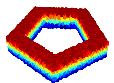
$t_{1}=0$

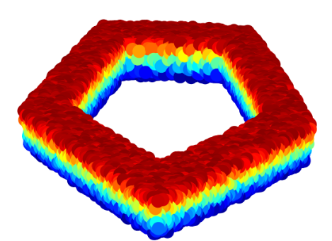
$t_{2}=0.1$

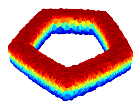
$t_{3}=0.2$

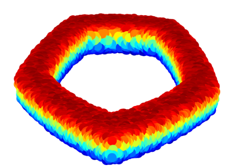
$t_{4}=0.4$

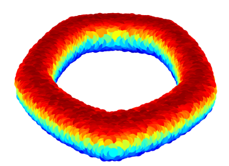
$t_{5}=0.6$

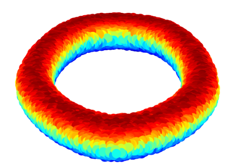
$t_{6}=0.8$

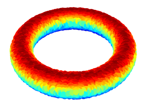
$t_{7}=1$

Figure 6: Metric measure spaces: Graphical illustration of the metric measure spaces $\left\{\mathcal{Y}_{i}\right\}_{i=1}^{7}$.

In this example, we are not interested in only finding local changes, but we want to distinguish between Euclidean metric measure spaces that differ globally. Hence, $m=1$ seems to be the most reasonable choice. At the end of this section, we will illustrate the influence of the parameter $m$ in the present setting. We draw independent samples of size $n$ from $\mu_{\mathcal{Y}_{i}}$, denoted as $\{Y_{j,n,i}\}_{j=1}^{n}$, and calculate $\Delta_{n,i}=\{{\delta}^{2}_{\mathcal{X},1}(Y_{j,n,i})\}_{j=1}^{n}$ and $\widehat{f}_{{\delta}^{2}_{{\mathcal{Y}_{i}},1}}$ based on each of these samples for $1\leq i\leq 7$ and $n=500,2500,5000,10000$ (Biweight kernel, $h_{i}=1.06\min\{s(\Delta_{n}),\text{IQR}(\Delta_{n})/1.34)\}n^{-1/5})$. We repeat this procedure for each $i$ and $n$ 10 times and display the resulting kernel density estimators in the upper row of Figure 7. While it is not possible to reliably distinguish between the realizations of $\widehat{f}_{{\delta}^{2}_{{\mathcal{Y}_{0}},1}}$ (blue-green), $\widehat{f}_{{\delta}^{2}_{{\mathcal{Y}_{1}},1}}$ (orange) and $\widehat{f}_{{\delta}^{2}_{{\mathcal{Y}_{2}},1}}$ (blue) by eye for $n=500$, this is very simple for $n\geq 2500$. Now, that we have estimated the densities, we can choose a suitable notion of distance between densities (e.g. the $L^{1}$-distance) and perform a linkage clustering in order to showcase that the illustrations in the upper row are not deceptive and that it is indeed possible to discriminate between the Euclidean metric measure spaces considered based on the kernel density estimators of the respective DTM-densities. To this end, we calculate the $L_{1}$-distance between the kernel density estimators considered and perform an average linkage clustering on the resulting distance matrix for each $n$. The results are showcased in the lower row of Figure 7. The average linkage clustering confirms our previous observations.

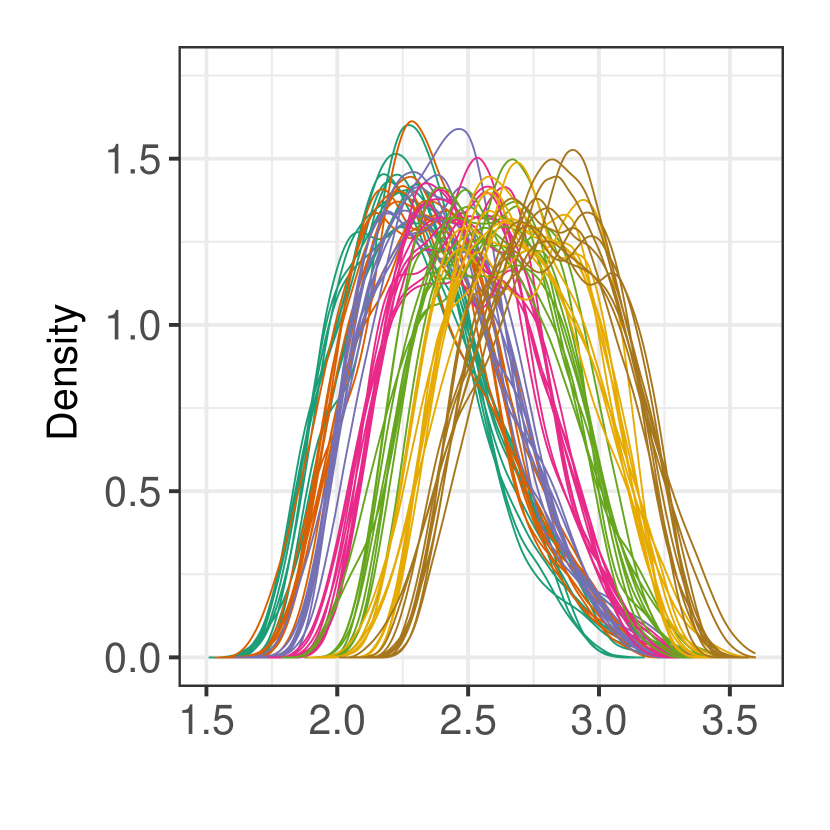
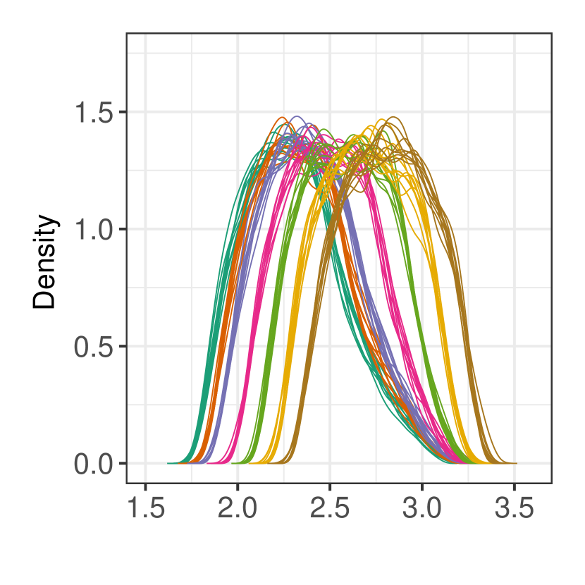
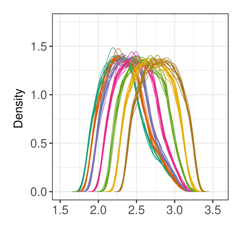
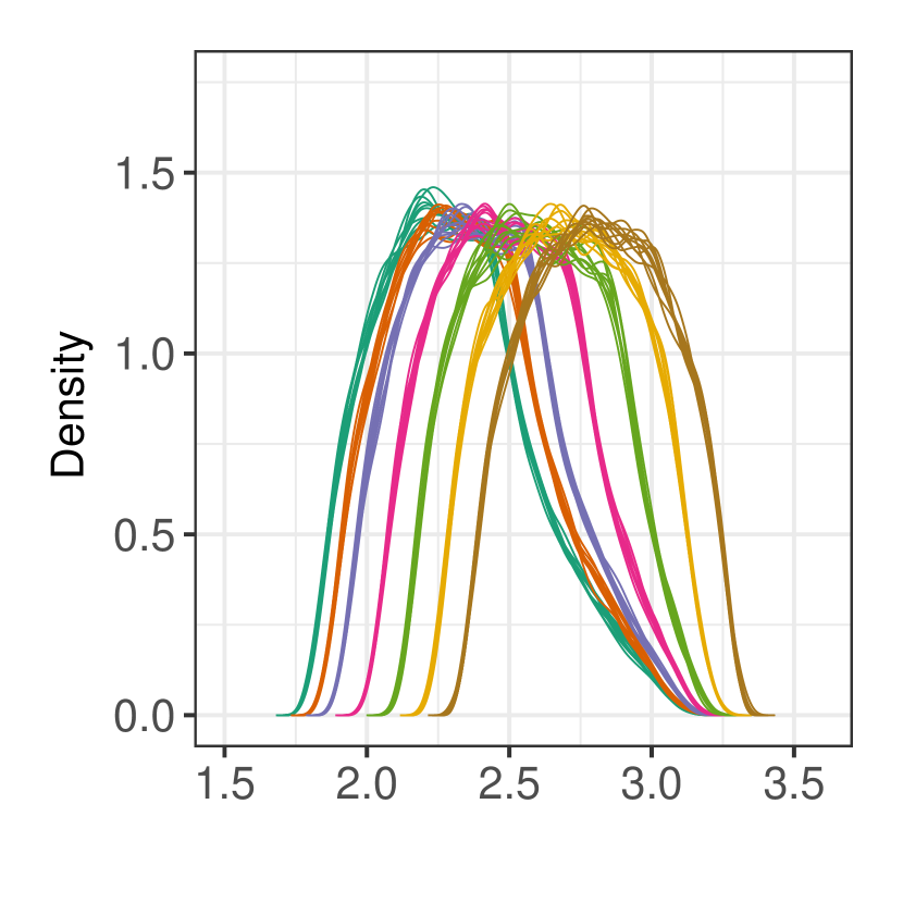
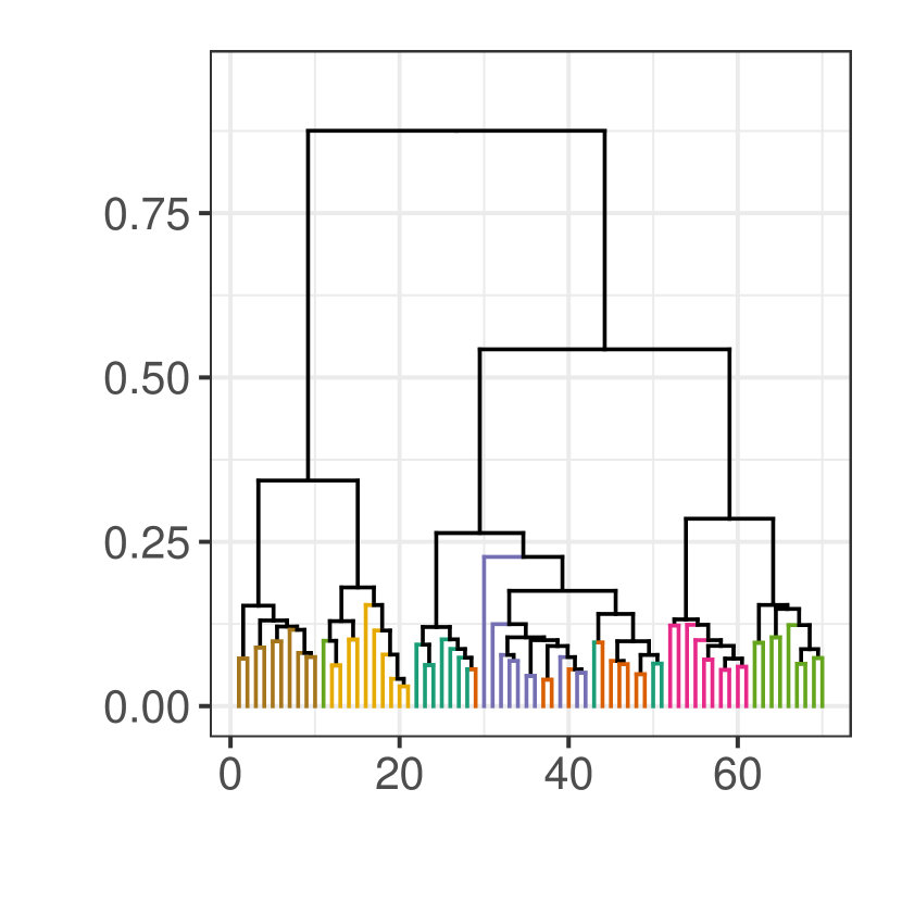
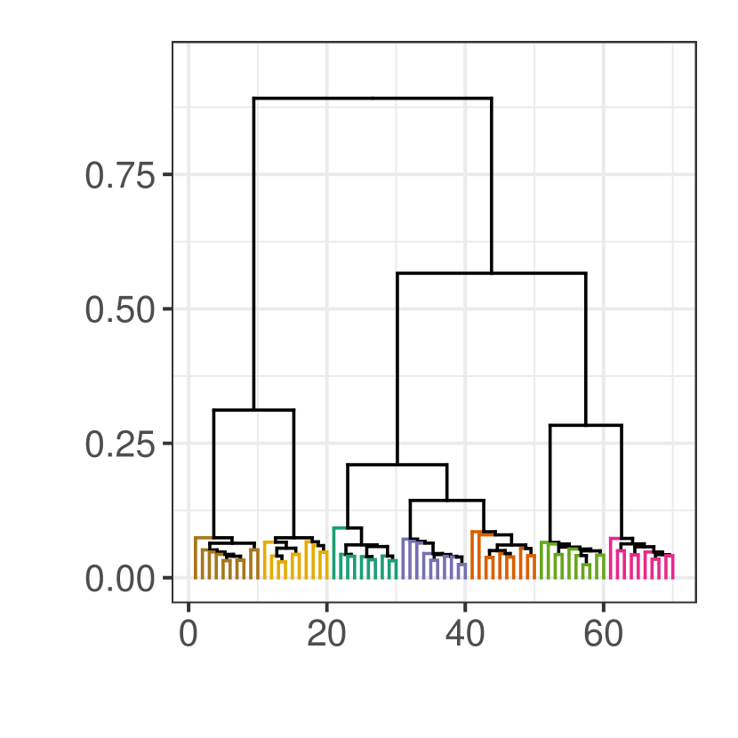
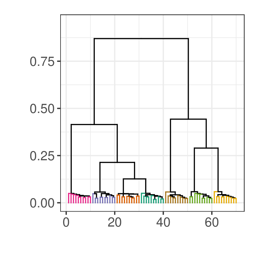
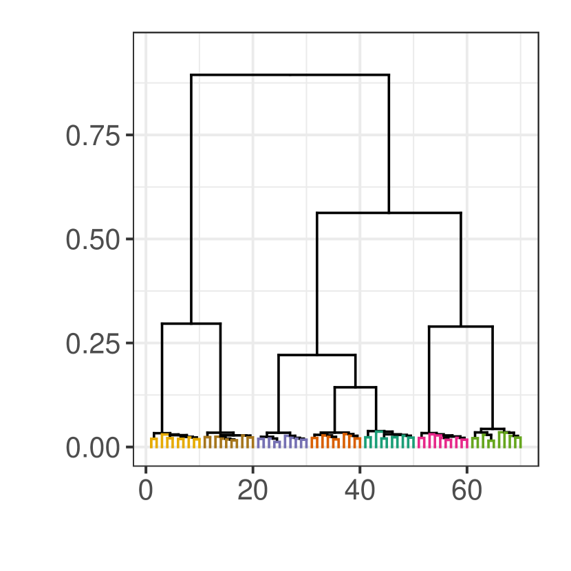
Figure 7: Discriminating between Euclidean metric measure spaces: Upper row: Ten realizations of the kernel density estimators $\widehat{f}_{{\delta}^{2}_{{\mathcal{Y}_{1}},1}}$ (blue-green), $\widehat{f}_{{\delta}^{2}_{{\mathcal{Y}_{2}},1}}$ (orange), $\widehat{f}_{{\delta}^{2}_{{\mathcal{Y}_{3}},1}}$ (blue), $\widehat{f}_{{\delta}^{2}_{{\mathcal{Y}_{4}},1}}$ (pink), $\widehat{f}_{{\delta}^{2}_{{\mathcal{Y}_{5}},1}}$ (green), $\widehat{f}_{{\delta}^{2}_{{\mathcal{Y}_{6}},1}}$ (yellow) and $\widehat{f}_{{\delta}^{2}_{{\mathcal{Y}_{6}},1}}$ (brown) for $n=500,2500,5000,10000$ (from left to right). Lower row: The results of an average linkage clustering of the considered kernel density estimators based on the $L^{1}$-distance (same coloring).

To conclude this section, we illustrate the influence of the choice of $m$. For this purpose, we repeat the above procedure with $n=10,000$ and $m=0.2,0.4,0.6,0.8$ (this means that we can use the alternative representation of $\mathrm{d}^{2}_{\mathcal{X},m}$ in (4) with $k=2000,4000,6000,8000$). The resulting kernel density estimators are displayed in the upper row and the corresponding average clustering in the bottom row of Figure 8 (same coloring as previously). As we consider the transformation of $\mu_{\mathcal{Y}_{1}}$ into $\mu_{\mathcal{Y}_{7}}$ along a 2-Wasserstein geodesic, it is intuitive that choosing $m$ too small is not informative in this setting (the goal is to distinguish between the whole spaces). Indeed, this is exactly, what we observe. For $m=0.2$ the kernel density estimators strongly resemble each other and in particular the Euclidean metric measure spaces $\mathcal{Y}_{1}$ and $\mathcal{Y}_{2}$ are hardly distinguishable (see the corresponding dendrogram in the lower row of Figure 8). For $m\geq 0.4$ the kernel density estimators are better separated and the corresponding dendrograms highlight that it possible to discriminate between the spaces $\mathcal{Y}_{i}$ based on the kernel density estimators $\widehat{f}_{{\delta}^{2}_{{\mathcal{Y}_{i}},m}}$, $i=1,\dots,7$ and $m=0.4,0.6,0.8$. It is noteworthy that although the form of the kernel density estimators drastically changes between $m=0.4$ and $m=1$, the quality of the corresponding clustering only increases slightly with increasing $m$.

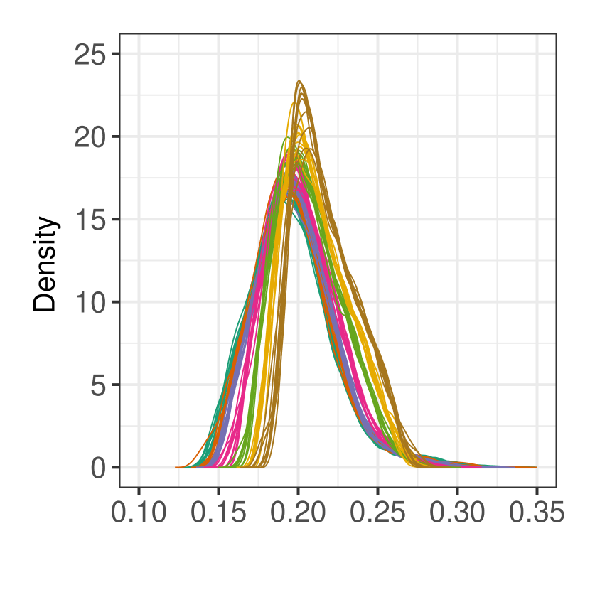
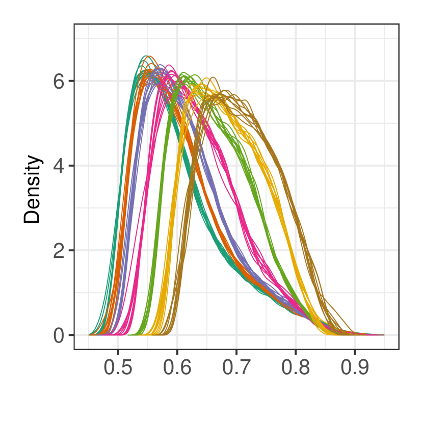
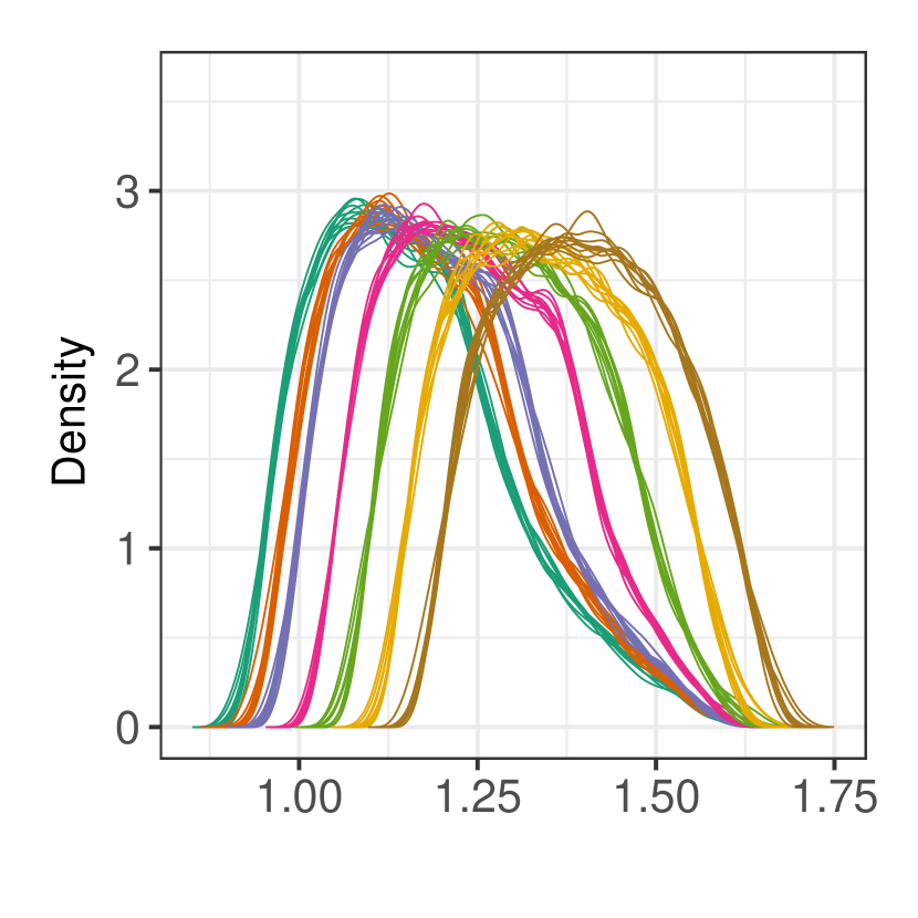
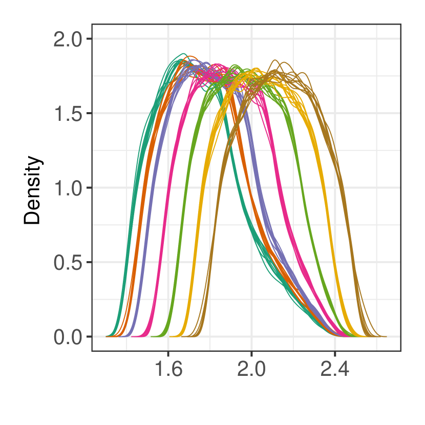
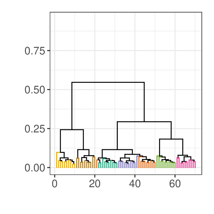
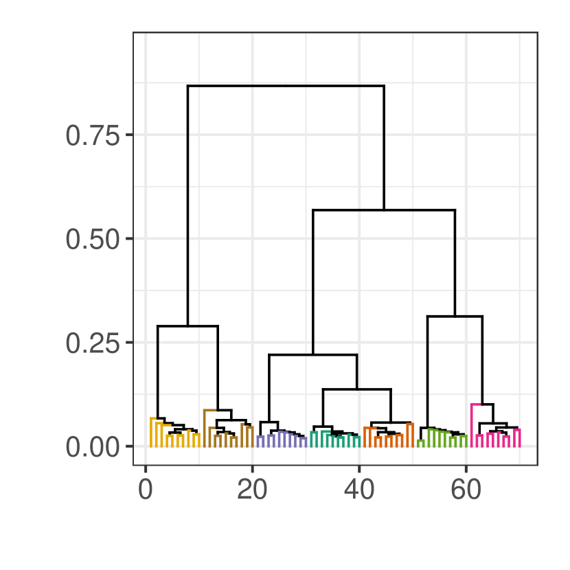
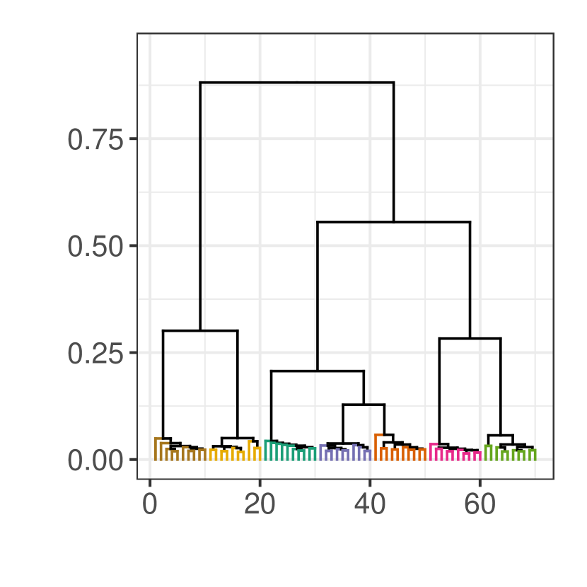
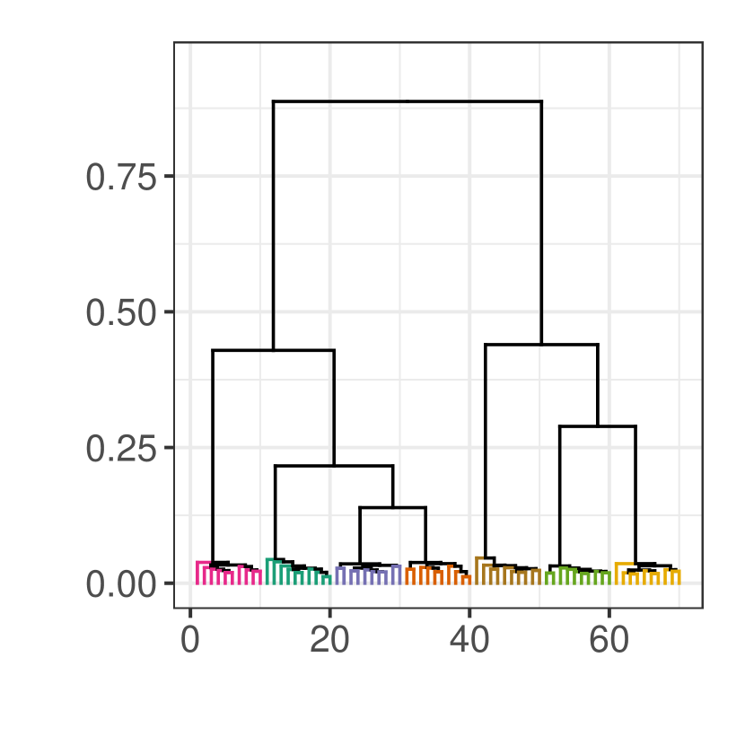
Figure 8: The influence of $m$: Upper row: Ten realizations of the kernel density estimators $\widehat{f}_{{\delta}^{2}_{{\mathcal{Y}_{1}},m}}$ (blue-green), $\widehat{f}_{{\delta}^{2}_{{\mathcal{Y}_{2}},m}}$ (orange), $\widehat{f}_{{\delta}^{2}_{{\mathcal{Y}_{3}},m}}$ (blue), $\widehat{f}_{{\delta}^{2}_{{\mathcal{Y}_{4}},m}}$ (pink), $\widehat{f}_{{\delta}^{2}_{{\mathcal{Y}_{5}},m}}$ (green), $\widehat{f}_{{\delta}^{2}_{{\mathcal{Y}_{6}},m}}$ (yellow) and $\widehat{f}_{{\delta}^{2}_{{\mathcal{Y}_{7}},m}}$ (brown) for $n=10000$ and $m=0.2,0.4,0.6,0.8$ (from left to right). Lower row: The results of an average linkage clustering of the considered kernel density estimators based on the $L^{1}$-distance (same coloring).

4 Chromatin Loop Analysis

In this section, we will highlight how to use the DTM-density-transformation for chromantin loop analysis. First, we briefly recall some important facts about chromatin fibers, state the goal of this analysis and precisely describe the data used here.

For human beings, chromosomes are essential parts of cell nuclei. They carry the genetic information important for heredity transmission and consist of chromatin fibers. Learning the topological 3D structure of the chromatin fiber in cell nuclei is important for a better understanding of the human genome. As discussed in Section 1.3, TADs are self-interacting genomic regions, which are often associated with loops in the chromatin fibers. These domains have been estimated to the range of 100–300 nm [43]. Hi-C data [33] allow to construct spatial proximity maps of the human genome and are often used to analyze genome-wide chromatin organization and to identify TADs. However, spatial size and form, and how frequently chromatin loops and domains exist in single cells, cannot directly be answered based on Hi-C data, whereas in 3D visualization of chromosomal regions via SMLM with a sufficiently high resolution, this information might be more easily accessible [26]. Therefore, in the above reference, such an approach is considered, in which two groups of images of chromatin fibers were produced: Chromatin with supposedly fully intact loop structures and chromatin, which had been treated with auxin prior to imaging. Auxin is known to cause a degrading of the loops. Therefore, in the second set of images, the loops are expected to be mostly dissolved. The obtained resolution in these images was of the order of 150 nm, i.e., below the diffraction limit and comparable to the typical sizes of TADs. This means that the analysis of chromatin loops based on these images is tractable but difficult as we will not see detailed loops when zooming in.

In this paper we analyse simulated SMLM data of chromatin fibers that mimic the chromatin structure with loops as local features and compare them to simulated data that mimic the progressive degradation of loop structures in five steps. The simulated structures mimic the first chromosome (of 23 in total) of the human genome, which is the longest with approximately 249 megabases (Mb, corresponding to 249,000,000 nucleotides). Each step corresponds to a loop density with a different parameter, which we denote by $c$. The value of $c$ is the number of loops per megabase. A value of $c=25$ corresponds to a high loop density with 2490 loops in total and corresponds to the setting without the application of auxin. Values of $c=10,6,4,2$ correspond to decreasing states of resolved loops (1494, 996 and 498 loops) and $c=0$ encodes the fully resolved state. These simulated images provide a controlled setting in which we can investigate the applicability of our methods and in which we can explore how small a difference in loop density our method can still pick up and when it starts to break down. Here, we only consider classification into the different conditions based on the estimated DTM density. While it is clear from the results described below that information on loop size and frequency is encoded in these densities, a quantification of these parameters requires a deeper study of the proposed methods and is beyond the scope of this manuscript.
In our study, we consider 102 synthetic, noisy samples of size 49800 of 6 different loop densities each and denote the corresponding samples as $\mathcal{X}_{i,c}$, $c=25,10,6,4,2,0$, $1\leq i\leq 102$. These samples are created by first discretizing the chromatin structure such that the distance between two points along the chromatin structure corresponds to $45$ nm. Then, we add independent, centered Gaussian errors with covariance matrix

$$\Sigma=\begin{pmatrix}45&0&0\\ 0&45&0\\ 0&0&90\end{pmatrix}$$

to each point (see Figure 9 for an illustration of data obtained in this fashion). This high level of noise is chosen to match the experimental data obtained in Hao et al. [26]. Throughout the following, we consider the data on a scale of 1:45. We stress once again that the goal of our analysis is to distinguish between the respective loop conditions and not between chromatin fibers from which the points are sampled (the overall form of the chromatin fibers within one condition can be quite different).

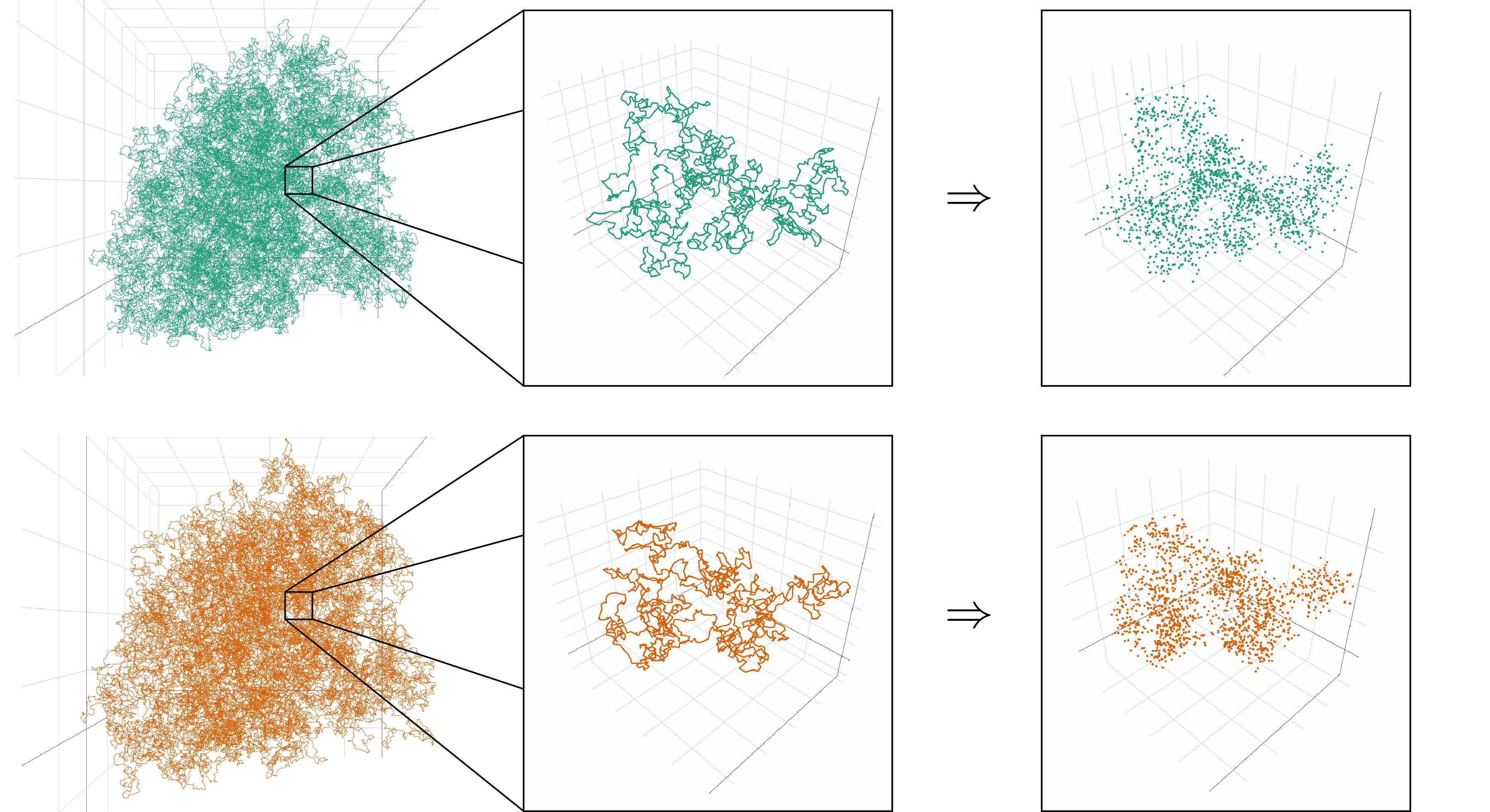
Figure 9: Chromatin Loops: Upper row: Illustration of a chromatin structure and the corresponding sample with loop density $c=25$. Lower row: Illustration of the same chromatin and the corresponding sample with loop density $c=10$.

We demonstrate in the following that the corresponding DTM-signatures, or more precisely the corresponding kernel density estimators $\widehat{f}_{{\delta}^{2}_{{\mathcal{X}_{i,c}},m}}$, $1\leq i\leq 102$, ($m$ chosen suitably small) represent a useful transformation of the data that allows discrimination between the different loop densities, while disregarding the overall shape of the chromatin fiber. To this end, we follow the strategy proposed in Section 1.3 and calculate $\Delta_{i,c}=\{{\delta}^{2}_{\mathcal{X},m}(X_{j,i,c}):X_{j,i,c}\in\mathcal{X}_{i,c}\}$ for $1\leq i\leq 102$, $c\in\{25,10,6,4,2,0\}$ and $m\in\{{1}/{9960},{1}/{4980},{1}/{1245}\}$. These particular choices of $m$ entail that in order to calculate ${\delta}^{2}_{\mathcal{X},m}(X_{j,i,c})$ we need to take the mean over the distances to the $k=5,10,40$ nearest neighbors of $X_{j,i,c}\in\mathcal{X}_{i,c}$ (recall the representation of ${\delta}^{2}_{\mathcal{X},m}$ in (4)). We determine $\widehat{f}_{{\delta}^{2}_{{\mathcal{X}_{i,c}},m}}$ based on each of the samples $\Delta_{i,c}$ (Biweight kernel, $h=1.06\min\{s(\Delta_{n}),\text{IQR}(\Delta_{n})/1.34)\}n^{-1/5})$. The resulting kernel density estimators are displayed in Figure 10. Generally, the kernel density estimators based on the different samples with the same loop density strongly resemble each other and it is possible to roughly distinguish between the different values of $c$. For all values of $m$ considered, the DTM-density estimators based on $\mathcal{X}_{i,25}$, $1\leq i\leq 102$, (here the respective chromatin fibers form many loops) are well separated from the other kernel density estimators and the estimators based on the samples $\Delta_{i,2}$ and $\Delta_{i,0}$ (which correspond to the lowest loop densities considered) are the most similar when comparing the different loop densities.

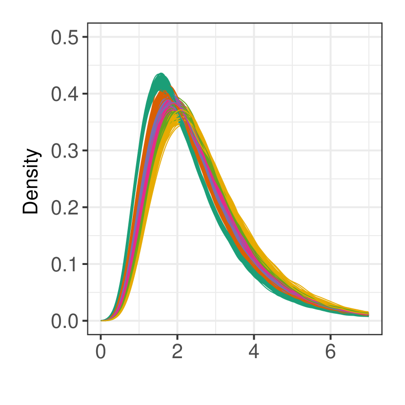
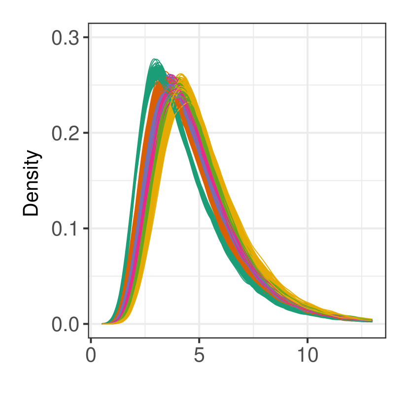
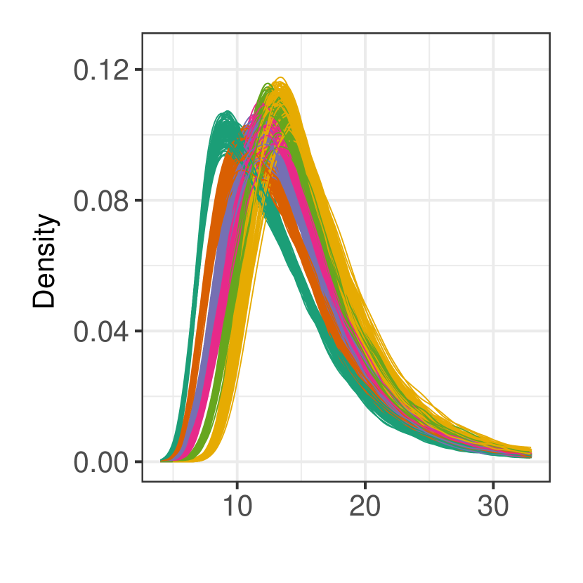
Figure 10: Chromatin Loop Analysis I: Illustration of the DTM-density estimators $\widehat{f}_{{\delta}^{2}_{{\mathcal{X}_{i,c}},m}}$, $1\leq i\leq 102$, for $c=25$ (blue-green), $c=10$ (orange), $c=6$ (blue), $c=4$ (pink), $c=2$ (green) and $c=0$ (yellow) and $m\in\{{1}/{9960},{1}/{4980},{1}/{1245}\}$ (from left to right).

In order to make a more qualitative comparison between the estimators $\widehat{f}_{{\delta}^{2}_{{\mathcal{X}_{i,c}},m}}$, we use the strategy developed in Section 3.2 and perform an average linkage clustering based on the $L_{1}$-distance between the estimated densities. For clarity, we restrict ourselves to the comparison of the loop density $c=25$ against $c=10$ as well as $c=2$ against $c=0$ and point out that the comparison between the setting $c=2$ against $c=0$ is very difficult as the loop frequencies are very low. The dendrograms in the upper row of Figure 11 illustrate the comparison of $c=25$ and $c=10$. It is remarkable that for each $m$ the correct clusters are obtained. The lower row of Figure 11 showcases the dendrograms for the comparison of the estimators $\widehat{f}_{{\delta}^{2}_{{\mathcal{X}_{i,2}},m}}$ and $\widehat{f}_{{\delta}^{2}_{{\mathcal{X}_{i,0}},m}}$, $1\leq i\leq 102$ and $m\in\{{1}/{9960},{1}/{4980},{1}/{1245}\}$. For $m\in\{{1}/{9960},{1}/{4980}\}$, we obtain (up to one exception) the correct clusters, although they are much closer (w.r.t. the $L^{1}$-distance) than the clusters for the previous comparisons. However, for $m={1}/{1245}$, it is no longer possible to reliably identify two clusters that correspond to $c=2$ and $c=0$. It seems that in this case $m$ is too large to yield a perfect discrimination.

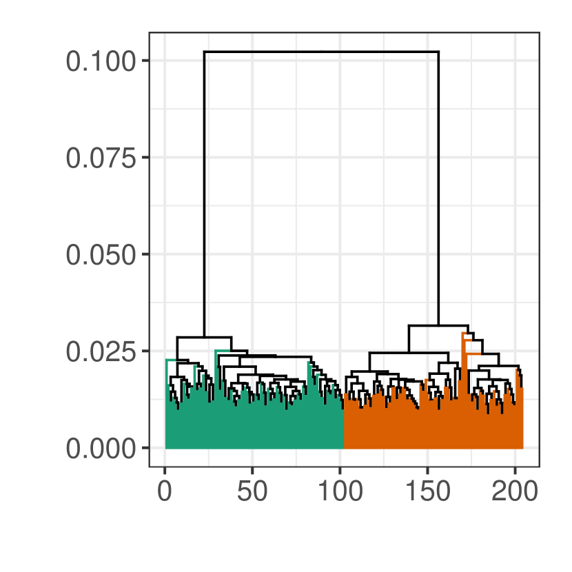
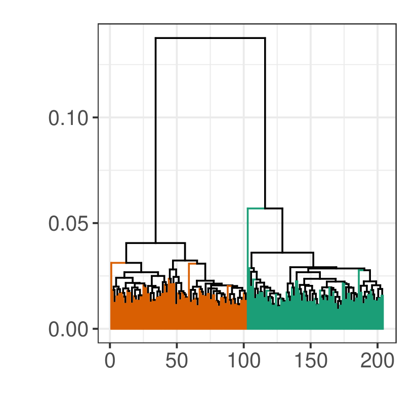
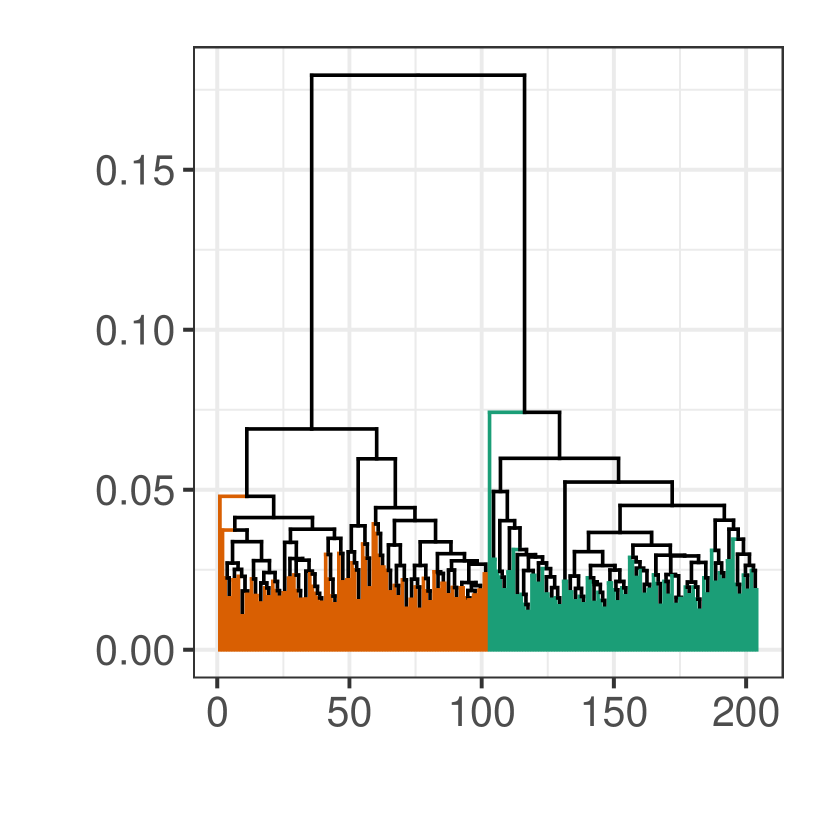
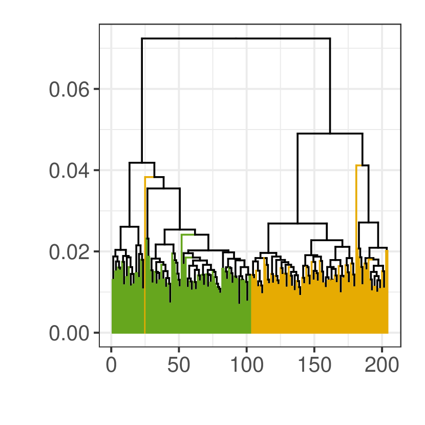
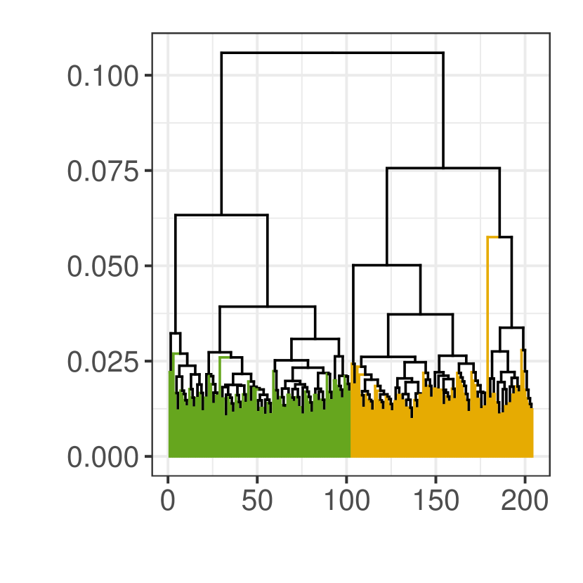
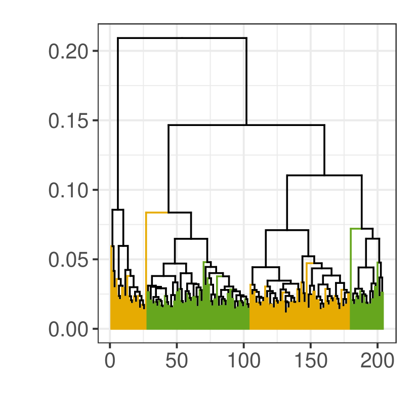
Figure 11: Chromatin Analysis II: Upper row: The results of an average linkage clustering of the kernel density estimators $\widehat{f}_{{\delta}^{2}_{{\mathcal{X}_{i,25}},m}}$ (blue-green) and $\widehat{f}_{{\delta}^{2}_{{\mathcal{X}_{i,10}},m}}$ (orange), $1\leq i\leq 102$, for $m\in\{{1}/{9960},{1}/{4980},{1}/{1245}\}$ (from left to right) based on the $L^{1}$-distance. Lower row: The results of an average linkage clustering of the kernel density estimators $\widehat{f}_{{\delta}^{2}_{{\mathcal{X}_{i,2}},m}}$ (green) and $\widehat{f}_{{\delta}^{2}_{{\mathcal{X}_{i,0}},m}}$ (yellow), $1\leq i\leq 102$, for $m\in\{{1}/{9960},{1}/{4980},{1}/{1245}\}$ (from left to right) based on the $L^{1}$-distance.

To conclude this section, we investigate whether classification based on the DTM-density estimates $\widehat{f}_{{\delta}^{2}_{{\mathcal{X}_{i,c}},m}}$ is possible. Here, we restrict ourselves once again to the comparison of $c=25$ with $c=10$ as well as of $c=2$ with $c=0$. For each comparison, we randomly select $5\%/10\%$ (rounded up) of the density estimates for each considered loop density and classify the remaining ones according to the the majority of the labels of their $k=1,3,5$ nearest neighbors in the randomly selected sample. We repeat this procedure for both comparisons 10,000 times and report the relative number of misclassifications in Table 1. The upper row of said table highlights that in the comparison of $c=25$ and $c=10$ the DTM-density estimates are always classified correctly. Things change in the comparison of $c=2$ with $c=0$. While for all $m$ at least $90\%$ of the classifications are correct, there is a noticeable difference between the individual values of $m$. We observe that $m={1}/{4980}$ yields by far the best performance in this setting. It is clear that the loop distributions of the respective chromatin fibers for these two parameters are extremely similar (the chromatin admits few to no loops). Hence, choosing $m$ too large incorporates too much global (non-loop) structure and makes it difficult to discriminate between these two loop densities. On the other hand, choosing $m$ too small seems to incorporate too little structure.

To conclude, we find that it is possible for a suitable choice of $m$ to clearly distinguish between the different loop densities based on the DTM-density estimators $\widehat{f}_{{\delta}^{2}_{{\mathcal{X}_{i,c}},m}}$. We have illustrated that these estimators yield a good summary of the data and can be used to approach the (already quite difficult) problem of chromatin loop analysis for noisy synthetic data.

	$k=1$	$k=3$	$k=5$
5%	0.000	0.000	0.000
10%	0.000	0.000	0.000

	$k=1$	$k=3$	$k=5$
5%	0.000	0.000	0.000
10%	0.000	0.000	0.000

	$k=1$	$k=3$	$k=5$
5%	0.000	0.000	0.000
10%	0.000	0.000	0.000

	$k=1$	$k=3$	$k=5$
5%	0.029	0.049	0.069
10%	0.020	0.033	0.043

	$k=1$	$k=3$	$k=5$
5%	0.012	0.019	0.039
10%	0.001	0.007	0.012

	$k=1$	$k=3$	$k=5$
5%	0.029	0.064	0.100
10%	0.008	0.021	0.025

Table 1: Chromatin Analysis III: Upper row: The relative number of missclassifications of a $k$-nearest neighbor classification (w.r.t. the $L^{1}$-distance) based on the kernel density estimators $\widehat{f}_{{\delta}^{2}_{{\mathcal{X}_{i,25}},m}}$ and $\widehat{f}_{{\delta}^{2}_{{\mathcal{X}_{i,10}},m}}$, $1\leq i\leq 102$, for $m\in\{{1}/{9960},{1}/{4980},{1}/{1245}\}$ (from left to right). Lower row: The relative number of missclassifications of a $k$-nearest neighbor classification (w.r.t. the $L^{1}$-distance) based on the kernel density estimators $\widehat{f}_{{\delta}^{2}_{{\mathcal{X}_{i,2}},m}}$ and $\widehat{f}_{{\delta}^{2}_{{\mathcal{X}_{i,0}},m}}$, $1\leq i\leq 102$, for $m\in\{{1}/{9960},{1}/{4980},{1}/{1245}\}$ (from left to right).

Appendix A Proof of Lemma 2.6

In this section, we state the full proof of Lemma 2.6.

Lemma 2.6.

Let $X=(X_{1},\dots,X_{d})\sim\mu_{\mathcal{X}}$ and $x=(x_{1},\dots,x_{d})\in\mathbb{R}^{d}$.

1. We observe that

   $$\mathrm{d}^{2}_{\mathcal{X},1}(x)=\mathbb{E}\left[||X-x||^{2}\right]= \sum_{i=1}^{d}\left(\mathbb{E}\left[X_{i}^{2}\right]-2x_{i}\mathbb{E}\left[X_{i}\right]+x_{i}^{2}\right)$$

   $$= \sum_{i=1}^{d}\left(\left(x_{i}-\mathbb{E}\left[X_{i}\right]\right)^{2}+\mathbb{E}\left[X_{i}^{2}\right]-(\mathbb{E}\left[X_{i}\right])^{2}\right).$$

   Setting $c_{i}=\mathbb{E}\left[X_{i}\right]$ and $\zeta=\sum_{i=1}^{d}\left(\mathbb{E}\left[X_{i}^{2}\right]-(\mathbb{E}\left[X_{i}\right])^{2}\right)$ yields the claim.

2. This follows directly from the fist statement.

3. The fist statement implies that

   $$\nabla\mathrm{d}^{2}_{\mathcal{X},1}(x)=2(x-\mathbb{E}\left[X\right]).$$

   Clearly, this is zero if and only if $x=\mathbb{E}\left[X\right]$.

4. By the second and third statement $\mathrm{d}^{2}_{\mathcal{X},1}$ is three times continuously differentiable and $\nabla\mathrm{d}^{2}_{\mathcal{X},1}>0$ on ${\mathrm{d}^{2}_{\mathcal{X},1}}^{-1}([y-2h_{0},y+2h_{0}])$. In consequence, there exists an open set $U\supset{\mathrm{d}^{2}_{\mathcal{X},1}}^{-1}([y-h_{0},y+h_{0}])$ such that the function

   $$\varphi:U\subset\mathbb{R}^{d}\to\mathbb{R}^{d};~{}x\mapsto\frac{\nabla\mathrm{d}^{2}_{\mathcal{X},1}(x)}{||\nabla\mathrm{d}^{2}_{\mathcal{X},1}(x)||^{2}}$$

   is $C^{2}(U,\mathbb{R}^{d})$. By Theorem 2 in Chapter 15 of Hirsch and Smale [29] there is a unique flow $\Phi^{*}:[-h_{0},h_{0}]\times W\to\mathbb{R}^{d}$ with

   $$\begin{cases}\frac{\partial}{\partial v}\Phi^{*}(v,x)=\frac{\nabla\mathrm{d}^{2}_{\mathcal{X},1}(\Phi^{*}(v,x))}{||\nabla\mathrm{d}^{2}_{\mathcal{X},1}(\Phi^{*}(v,x))||^{2}}\\ \Phi^{*}(0,x)=x,\end{cases}$$ (17)

   where $W\subset\mathbb{R}^{d}$ is an open set that contains ${\mathrm{d}^{2}_{\mathcal{X},1}}^{-1}([y-h_{0},y+h_{0}])$. Differentiating the function $v\mapsto\mathrm{d}^{2}_{\mathcal{X},1}(\Phi^{*}(v,x))$ immediately shows that $\mathrm{d}^{2}_{\mathcal{X},1}\left(\Phi^{*}(v,x)\right)=\mathrm{d}^{2}_{\mathcal{X},1}(x)+v$. This implies that $\Phi^{*}(v,{\mathrm{d}^{2}_{\mathcal{X},1}}^{-1}(\{y\}))={\mathrm{d}^{2}_{\mathcal{X},1}}^{-1}(\{y+v\})$. In consequence, it only remains prove that $\Phi$ defined in the statement is a solution of the ordinary differential equation (17). For this purpose, we observe that $\Phi(0,x)=x$ for all $x$. Furthermore, we derive that

   $$\frac{\partial}{\partial v}\Phi(v,x)=\left(\frac{x_{1}-c_{1}}{2||x-c||^{2}\sqrt{\frac{v}{||x-c||^{2}}+1}},\dots,\frac{x_{d}-c_{d}}{2||x-c||^{2}\sqrt{\frac{v}{||x-c||^{2}}+1}}\right)^{T}$$

   By the first statement, it follows immediately that

   $$\frac{\nabla\mathrm{d}^{2}_{\mathcal{X},1}(x)}{||\nabla\mathrm{d}^{2}_{\mathcal{X},1}(x)||^{2}}=\left(\frac{x_{1}-c_{1}}{2||x-c||^{2}},\dots,\frac{x_{d}-c_{d}}{2||x-c||^{2}}\right)^{T}.$$

   In consequence, we find that

   $$\frac{\nabla\mathrm{d}^{2}_{\mathcal{X},1}(\Phi^{*}(v,x))}{||\nabla\mathrm{d}^{2}_{\mathcal{X},1}(\Phi^{*}(v,x))||^{2}}=\left(\frac{x_{1}-c_{1}}{2||x-c||^{2}\sqrt{\frac{v}{||x-c||^{2}}+1}},\dots,\frac{x_{d}-c_{d}}{2||x-c||^{2}\sqrt{\frac{v}{||x-c||^{2}}+1}}\right)^{T},$$

   which proves the fourth statement.

∎

Appendix B Additional Details on Example 2.7-2.10

In this section, we will provide additional details on the examples considered in Section 2.2. For each example considered, we first briefly recall the setting and derive the corresponding DTM-function and DTM-density.

B.1 Example 2.8

Let $\mathcal{X}=[0,1]$ and let $\mu_{\mathcal{X}}$ denote the uniform distribution on $\mathcal{X}$. Furthermore, we consider two values for $m$, namely $m_{1}=1$ and $m_{2}=0.1$.

First, we derive $\mathrm{d}^{2}_{\mathcal{X},1}$ and $f_{\mathrm{d}^{2}_{\mathcal{X},1}}$. To this end, we observe that for $x\in\mathcal{X}$ and $X\sim\mu_{\mathcal{X}}$

$$\mathrm{d}^{2}_{\mathcal{X},1}(x)=\int_{0}^{1}\!F_{x}^{-1}(t)\,dt=\mathbb{E}\left[(X-x)^{2}\right]=\frac{1}{3}-x+x^{2}.$$

This immediately gives that

$$F_{\mathrm{d}^{2}_{\mathcal{X},1}}(t)=\mathbb{P}\left(\mathrm{d}^{2}_{\mathcal{X},1}(X)\leq t\right)=\begin{cases}0&t\leq\frac{1}{12},\\ \sqrt{4t-\frac{1}{3}}&\frac{1}{12}\leq t\leq\frac{1}{3},\\ 1&t>\frac{1}{3}.\end{cases}$$

Hence, $f_{\mathrm{d}^{2}_{\mathcal{X},1}}$ is given as

$$f_{\mathrm{d}^{2}_{\mathcal{X},1}}(t)=\begin{cases}\frac{2\sqrt{3}}{\sqrt{12t-1}}&\frac{1}{12}\leq t\leq\frac{1}{3},\\ 0&\,\text{else.}\end{cases}$$

Next, we come to $m_{2}=0.1$. In order to calculate $\mathrm{d}^{2}_{\mathcal{X},0.1}$ and $f_{\mathrm{d}^{2}_{\mathcal{X},0.1}}$, it is necessary to derive the family $\left(F_{x}^{-1}\right)_{x\in\mathcal{X}}$ explicitly. A short calculation yields that for $0\leq x\leq 1/2$

$$F_{x}^{-1}(y)=\begin{cases}\frac{y^{2}}{4}&0<y\leq 2x,\\ (y-x)^{2}&2x<y<1,\end{cases}$$

and for $1/2<x\leq 1$

$$F_{x}^{-1}(y)=\begin{cases}\frac{y^{2}}{4}&0<y\leq 2(1-x),\\ (y-(1-x))^{2}&2(1-x)<y<1.\end{cases}$$

Therefore, we find that

$$\mathrm{d}^{2}_{\mathcal{X},0.1}(x)=\begin{cases}x^{2}+0.1x+\frac{1}{300}&0\leq x<0.05,\\ \frac{1}{1200}&0.05\leq x\leq 0.95,\\ (1-x)^{2}+0.1(1-x)+\frac{1}{300}&0.95\leq x\leq 1.\\ \end{cases}$$

Since $\mathrm{d}^{2}_{\mathcal{X},0.1}$ is constant for $x\in[0.05,0.95]$ it is immediately clear that the corresponding distribution function $F_{\mathrm{d}^{2}_{\mathcal{X},0.1}}$ is not continuous. Indeed, we find that

$$F_{\mathrm{d}^{2}_{\mathcal{X},0.1}}(y)=\mathbb{P}\left(\mathrm{d}^{2}_{\mathcal{X},0.1}(X)\leq y\right)=\begin{cases}0&y<\frac{1}{1200},\\ \frac{1}{20}\sqrt{400y-\frac{1}{3}}+0.9&\frac{1}{1200}\leq y\leq\frac{1}{300},\\ 1&y\geq\frac{1}{300}.\\ \end{cases}$$

B.2 Example 2.9

Let $\mathcal{X}=[0,1]$ and let $\mu_{\mathcal{X}}$ denote the probability distribution on $[0,1]$ with density $f(x)=2x$. Let $m=0.1$. As previously, we have to explicitly calculate the family $\left(F_{x}^{-1}\right)_{x\in\mathcal{X}}$. A short calculation shows that for $0\leq x\leq 1/2$ we have that

$$F_{x}^{-1}(y)=\begin{cases}\frac{y^{2}}{16x^{2}}&0<y\leq 4x^{2},\\ (\sqrt{y}-x)^{2}&4x^{2}<y<1,\end{cases}$$

and for $1/2<x\leq 1$

$$F_{x}^{-1}(y)=\begin{cases}\frac{y^{2}}{16x^{2}}&0<y\leq 4x(1-x),\\ (x-\sqrt{1-y})^{2}&4x(1-x)<y<1.\end{cases}$$

The integration of these function on $[0,0.1]$, shows that the corresponding DTM-function is given as

$$\mathrm{d}^{2}_{\mathcal{X},0.1}(x)=\begin{cases}x^{2}-\frac{2}{3}\sqrt{\frac{2}{5}}x+\frac{1}{20}&0\leq x\leq\frac{\sqrt{0.1}}{2},\\ \frac{1}{4800x^{2}}&\frac{\sqrt{0.1}}{2}\leq x\leq\frac{1}{2}+\frac{3}{2\sqrt{10}},\\ x^{2}+\left(18\sqrt{\frac{2}{5}}-\frac{40}{3}\right)x+\frac{19}{20}&\frac{1}{2}+\frac{3}{2\sqrt{10}}<x\leq 1.\\ \end{cases}$$

It is obvious that in this case $\mathrm{d}^{2}_{\mathcal{X},0.1}$ is almost nowhere constant. Furthermore, we can now show that

$$F_{\mathrm{d}^{2}_{\mathcal{X},0.1}}(y)=\begin{cases}0&y\!\leq-\frac{13661}{180}\!+24\sqrt{10},\vspace{2mm}\\ \frac{2}{45}\left(-27\sqrt{2}+20\sqrt{5}\right)\sqrt{13661-4320\sqrt{10}+180y}&-\frac{13661}{180}\!+24\sqrt{10}<\!y\!\leq\frac{19-6\sqrt{10}}{120},\vspace{2mm}\\ \begin{subarray}{c}y-\frac{3}{5}\sqrt{360y-8640\sqrt{10}+27322}+\frac{4}{9}\sqrt{900y-21600\sqrt{10}+68305}\\ -\frac{1}{4800y}-48\sqrt{10}+\frac{27493}{180}\end{subarray}&\frac{19-6\sqrt{10}}{120}<y\leq\frac{-683}{60}+18\sqrt{\frac{2}{5}},\vspace{2mm}\\ 1-\frac{1}{4800y}&\,\frac{-683}{60}+18\sqrt{\frac{2}{5}}<\!y\!\leq\frac{1}{120}\vspace{2mm}\\ -y+\frac{1}{45}\sqrt{360y-2}+\frac{173}{180}&\,\frac{1}{120}<\!y\!\leq\frac{1}{20}\vspace{2mm}\\ 1&y\!>\frac{1}{20}.\end{cases}$$

This allows us to derive that

$$f_{\mathrm{d}^{2}_{\mathcal{X},0.1}}(y)=\begin{cases}\frac{80\sqrt{5}-108\sqrt{2}}{\sqrt{13661-4320\sqrt{10}+180y}}&-\frac{13661}{180}+24\sqrt{10}<y\leq\frac{19-6\sqrt{10}}{120},\vspace{2mm}\\ 1+\frac{40\sqrt{5}-54\sqrt{2}}{\sqrt{13661-4320\sqrt{10}+180y}}+\frac{1}{4800y^{2}}&\frac{19-6\sqrt{10}}{120}<y\leq\frac{-683}{60}+18\sqrt{\frac{2}{5}},\vspace{2mm}\\ \frac{1}{4800y^{2}}&\,\frac{-683}{60}+18\sqrt{\frac{2}{5}}<y\leq\frac{1}{120}\vspace{2mm}\\ -1+\frac{2}{\sqrt{-\frac{1}{2}+90y}}&\,\frac{1}{120}<y\leq\frac{1}{20}\vspace{2mm}\\ 0&\text{else}.\end{cases}$$

B.3 Example 2.7

Let $\mathcal{X}=[0,1]^{2}$ and let $\mu_{\mathcal{X}}$ stand for the uniform distribution on $\mathcal{X}$. Choose $m=1$ and let $\mathcal{X}\sim\mu_{\mathcal{X}}$. Then, it is possible to derive that for $x=(x_{1},x_{2})\in\mathcal{X}$

$$\mathrm{d}^{2}_{\mathcal{X},1}(x)=\mathbb{E}\left[||X-x||^{2}\right]=x_{1}^{2}+x_{2}^{2}-x_{1}-x_{2}+\frac{2}{3}.$$

Hence, we find that

$$F_{\mathrm{d}^{2}_{\mathcal{X},1}}(y)=\begin{cases}0&y\leq\frac{1}{6},\vspace{2mm}\\ \pi\left(y-\frac{1}{6}\right)&\frac{1}{6}<y\leq\frac{5}{12},\vspace{2mm}\\ \begin{subarray}{c}\frac{1}{3}\big{(}\sqrt{36y-15}+(6y-1)\mathrm{arccot}\left(2\sqrt{y-\frac{5}{12}}\right)\\ +(1-6y)\arctan\left(\sqrt{4y-\frac{5}{3}}\right)\big{)}\end{subarray}&\frac{5}{12}<y\leq\frac{2}{3},\vspace{2mm}\\ 1&\,y>\frac{2}{3}.\end{cases}$$

The corresponding density is given as

$$f_{\mathrm{d}^{2}_{\mathcal{X},1}}(y)=\begin{cases}\pi&\frac{1}{6}\leq y\leq\frac{5}{12},\\ 2\mathrm{arccot}\left(2\sqrt{y-\frac{5}{12}}\right)-2\arctan\left(\sqrt{4y-\frac{5}{3}}\right)&\frac{5}{12}<y\leq\frac{2}{3},\\ 0&\,\text{else.}\end{cases}$$

B.4 Example 2.10

Let $\mathcal{X}$ denote a disk in $\mathbb{R}^{2}$ centered at $(0,0)$ with radius 1 and let $\mu_{\mathcal{X}}$ denote probability measure with density

$$f(x_{1},x_{2})=\begin{cases}-\frac{2}{\pi}\left(x_{1}^{2}+x_{2}^{2}-1\right)&x_{1}^{2}+x_{2}^{2}\leq 1,\\ 0&\,\text{else.}\end{cases}$$

In this case, it is for $m=1$ straight forward to derive that for $x=(x_{1},x_{2})\in\mathcal{X}$

$$\mathrm{d}^{2}_{\mathcal{X},1}(x)=x_{1}^{2}+x_{2}^{2}+\frac{1}{3}.$$ (18)

In consequence, we find that for $X\sim\mu_{\mathcal{X}}$

$$F_{\mathrm{d}^{2}_{\mathcal{X},1}}(y)=\begin{cases}0&y\leq\frac{1}{3},\\ -y^{2}+\frac{8}{3}y-\frac{7}{9}&\frac{1}{3}<y\leq\frac{4}{3},\\ 1&\,\text{else.}\end{cases}$$

The corresponding density is given as

$$f_{\mathrm{d}^{2}_{\mathcal{X},1}}(y)=\begin{cases}-2y+\frac{8}{3}&\frac{1}{3}<y\leq\frac{4}{3},\\ 0&\,\text{else.}\end{cases}$$ (19)

Appendix C Proof of Theorem 2.12

In this section, we give the full proof of Theorem 2.12. The proof is composed of four steps, each of which formulated as an independent lemma (see Section C.1).

• Step 1: Replacement of ${\delta}^{2}_{\mathcal{X},m}(X_{i})$ by $\mathrm{d}^{2}_{\mathcal{X},m}(X_{i})$ (Lemma C.1).
  We provide a decomposition of $\widehat{f}_{{\delta}^{2}_{\mathcal{X},m}}$ in a sum of two leading terms in which ${\delta}^{2}_{\mathcal{X},m}(X_{i})$ is replaced by $\mathrm{d}^{2}_{\mathcal{X},m}(X_{i})$ in the argument of the kernel $K$ and we show that the remainder terms are negligible.

• Step 2: Introducing U-statistics (Lemma C.2).
  It is shown that the leading terms obtained in Step 1 can be written as a (sum of two) U-statistic(s) asymptotically.

• Step 3: Hoeffding decomposition (Lemma C.4).
  Applying a Hoeffding decomposition allows to derive a representation of the (sum of two) U-statistic(s) of step 2 as a sum of a deterministic term (expectation), a stochastic leading term consisting of a sum of independent random variables and a remainder term.

• Step 4: CLT for the leading term of Step 3 (Lemma C.7).
  Since the leading term of Step 3 is a sum of centered independent random variables, we can apply a standard CLT to show its asymptotic normality.

C.1 Auxiliary lemmas representing Step 1 - Step 4

Before we come to the proof of Theorem 2.12, we will establish several auxiliary results. In order to highlight the overall proof strategy, the corresponding proofs are deferred to Section C.3. We begin this section, by addressing Step 1.

Lemma C.1 (Step 1).

Assume that Setting 2.1 holds and let Condition 2.2 be met. Then, it follows that

$$\widehat{f}_{{\delta}^{2}_{\mathcal{X},m}}(y)=\frac{1}{n}\sum_{i=1}^{n}\left[\frac{1}{h}K\left(\frac{\mathrm{d}^{2}_{\mathcal{X},m}(X_{i})-y}{h}\right)+\frac{1}{h^{2}}K^{\prime}\left(\frac{\mathrm{d}^{2}_{\mathcal{X},m}(X_{i})-y}{h}\right)A_{n}(X_{i})\right]$$

$$+\mathcal{O}_{P}\left(\frac{1}{nh^{3}}\right)+o_{P}\left(\frac{\log(n)^{1/(2b)}}{n^{1/2+1/(2b)}h}\right),$$

where

$$A_{n}(x)\coloneqq\frac{1}{m}\int_{0}^{F_{x}^{-1}(m)}\!F_{x}(t)-\widehat{F}_{x,n}(t)\,dt.$$

As a direct consequence of Lemma C.1, we find that for $h\in o\left(1/n^{1/5}\right)$ the statistic

$$V_{n}(y)=\frac{1}{n}\sum_{i=1}^{n}\frac{1}{h}K\left(\frac{\mathrm{d}^{2}_{\mathcal{X},m}(X_{i})-y}{h}\right)+\frac{1}{n}\sum_{i=1}^{n}\frac{1}{h^{2}}K^{\prime}\left(\frac{\mathrm{d}^{2}_{\mathcal{X},m}(X_{i})-y}{h}\right)A_{n}(X_{i})$$

$$\eqqcolon V_{n}^{(1)}(y)+V_{n}^{(2)}(y)$$ (20)

drives the limit behavior of $\sqrt{nh}\left(\widehat{f}_{{\delta}^{2}_{\mathcal{X},m}}(y)-f_{\mathrm{d}^{2}_{\mathcal{X},m}}(y)\right)$. Next, we will establish that the statistic $V_{n}(y)$ can, up to asymptotically negligible terms, be written as a $U$-statistic (see e.g. Van der Vaart [52] for more information on $U$-statistics).

Lemma C.2 (Introduction of U-statistics, Step 2).

Assume Setting 2.1 and let $V_{n}^{(1)}$ and $V_{n}^{(2)}$ be as defined in (20). Then, we have

$$V_{n}^{(1)}(y)=\frac{2}{n(n-1)}\sum_{1\leq i<j\leq n}g^{(1)}_{y,h}(X_{i},X_{j}),$$

where

$$g^{(1)}_{y,h}(x_{1},x_{2})=\frac{1}{2h}\left(K\left(\frac{\mathrm{d}^{2}_{\mathcal{X},m}(x_{1})-y}{h}\right)+K\left(\frac{\mathrm{d}^{2}_{\mathcal{X},m}(x_{2})-y}{h}\right)\right).$$

Furthermore,

$$V_{n}^{(2)}(y)=\frac{2}{n(n-1)}\sum_{1\leq i<j\leq n}g^{(2)}_{y,h}(X_{i},X_{j})+\mathcal{O}_{P}\left(\frac{1}{nh^{2}}\right),$$

where

$$g^{(2)}_{y,h}(x_{1},x_{2})= \frac{1}{2mh^{2}}\Bigg{[}K^{\prime}\left(\frac{\mathrm{d}^{2}_{\mathcal{X},m}(x_{1})-y}{h}\right)\int_{0}^{F_{x_{1}}^{-1}(m)}\!F_{x_{1}}(t)-\mathds{1}_{\{||x_{1}-x_{2}||^{2}\leq t\}}\,dt$$

$$+K^{\prime}\left(\frac{\mathrm{d}^{2}_{\mathcal{X},m}(x_{2})-y}{h}\right)\int_{0}^{F_{x_{2}}^{-1}(m)}\!F_{x_{2}}(t)-\mathds{1}_{\{||x_{1}-x_{2}||^{2}\leq t\}}\,dt\Bigg{]}.$$

Remark C.3.

It is important to note that $g^{(1)}_{y,h}$ and $g^{(2)}_{y,h}$ are symmetric by definition, i.e., $V_{n}^{(1)}(x)$ is a $U$-statistic and $V_{n}^{(2)}(x)$ can be decomposed into a U-statistic and an asymptotically negligible remainder term.

Combining Lemma C.1 and Lemma C.2, we see that

$$\widehat{f}_{{\delta}^{2}_{\mathcal{X},m}}(y)=U_{n}+\mathcal{O}_{P}\left(\frac{1}{nh^{3}}\right)+o_{P}\left(\frac{\log(n)^{1/(2b)}}{n^{1/2+1/(2b)}h}\right),$$ (21)

where $U_{n}=U_{n}(y)$ denotes the $U$-statistic with kernel function $g_{y,h}(x_{1},x_{2})\coloneqq g^{(1)}_{y,h}(x_{1},x_{2})+g^{(2)}_{y,h}(x_{1},x_{2})$. Before we use (21) to finalize the proof of Theorem 2.12, we establish two further auxiliary results. Next, we rewrite $U_{n}$ using the Hoeffding decomposition (see Van der Vaart [52, Sec. 11.4]), which is the key ingredient to handling the stochastic dependencies introduced by the terms $A_{n}(X_{i})$.

Lemma C.4 (Hoeffding decomposition, Step 3).

Assume Setting 2.1. Let $U_{n}$ be the $U$-statistic with kernel function $g_{y,h}(x_{1},x_{2})=g^{(1)}_{y,h}(x_{1},x_{2})+g^{(2)}_{y,h}(x_{1},x_{2})$. Then, it follows that

$$U_{n}=\Theta_{y,h}+\frac{2}{n}\sum_{i=1}^{n}g_{y,h,1}(X_{i})+\frac{2}{n(n-1)}\sum_{1\leq i<j\leq n}g_{y,h,2}(X_{i},X_{j}).$$

Here, we have that

$$\Theta_{y,h}=\int\!K\left(v\right)f_{\mathrm{d}^{2}_{\mathcal{X},m}}(x+vh)\,dv.$$

Furthermore, let $Z_{1},Z_{2}\overset{i.i.d.}{\sim}\mu_{\mathcal{X}}$. Then, it holds that

$$g_{y,h,1}(x_{1})= \frac{1}{2h}K\left(\frac{\mathrm{d}^{2}_{\mathcal{X},m}(x_{1})-y}{h}\right)-\frac{1}{2}\Theta_{y,h}+\mathbb{E}_{Z_{1}}\left[\frac{1}{2mh^{2}}K^{\prime}\left(\frac{\mathrm{d}^{2}_{\mathcal{X},m}(Z_{1})-y}{h}\right)\Psi(x_{1},Z_{1})\right],$$

where

$$\Psi(x_{1},x_{2})\coloneqq||x_{1}-x_{2}||^{2}\wedge{F_{x_{2}}^{-1}(m)}-\mathbb{E}_{Z_{2}}\left[||Z_{2}-x_{2}||^{2}\wedge{F_{x_{2}}^{-1}(m)}\right],$$ (22)

and

$$g_{y,h,2}(x_{1},x_{2})=g_{y,h}(x_{1},x_{2})-g_{y,h,1}(x_{1})-g_{y,h,1}(x_{2})-\Theta_{y,h}.$$ (23)

Remark C.5.

It is well known that the mean zero random variables $\left(g_{y,h,2}(X_{i},X_{j})\right)_{1\leq i<j\leq n}$ are uncorrelated (see Van der Vaart [52, Sec. 11.4]).

For our later considerations it is important to derive a certain regularity for the function $\Psi$ defined in (22).

Lemma C.6.

Assume Setting 2.1 and let $\Psi$ be the function defined in (22). Then, the function $z\mapsto\Psi(x_{1},z)$ is Lipschitz continuous for all $x_{1}\in\mathcal{X}$ and the corresponding Lipschitz constant does not depend on the choice of $x_{1}$, i.e., it holds

$$\left|\Psi(x_{1},z_{1})-\Psi(x_{1},z_{2})\right|\leq C||z_{1}-z_{2}||,$$

for all $z_{1},z_{2}\in\mathcal{X}$, where the constant $0<C<\infty$ does not depend on $x_{1}$.

The next step in the proof of Theorem 2.12 is to derive for $n\to\infty$ and $h\to 0$ the limit distribution of $\sqrt{nh}\big{(}\frac{2}{{n}}\sum_{i=1}^{n}g_{y,h,1}(X_{i})\big{)}$.

Lemma C.7.

Assume Setting 2.1 and let Condition 2.2 be met. Let $n\to\infty,h\to 0$ such that $nh\to\infty$ and recall that

$$g_{y,h,1}(x_{1})= \frac{1}{2h}K\left(\frac{\mathrm{d}^{2}_{\mathcal{X},m}(x_{1})-y}{h}\right)-\frac{1}{2}\Theta_{y,h}+\mathbb{E}_{Z_{1}}\left[\frac{1}{2mh^{2}}K^{\prime}\left(\frac{\mathrm{d}^{2}_{\mathcal{X},m}(Z_{1})-y}{h}\right)\Psi(x_{1},Z_{1})\right],$$

It holds

$$\frac{2\sqrt{h}}{\sqrt{n}}\sum_{i=1}^{n}g_{y,h,1}(X_{i})\Rightarrow N\left(0,f_{\mathrm{d}^{2}_{\mathcal{X},m}}(y)\int\!K^{2}(u)\,du\right).$$ (24)

With all auxiliary results required established, we can finally come to the proof of Theorem 2.12. The proof strategy is to demonstrate that the limit of $\sqrt{nh}\left(\widehat{f}_{{\delta}^{2}_{\mathcal{X},m}}(y)-f_{\mathrm{d}^{2}_{\mathcal{X},m}}(y)\right)$ coincides with the limit of $\frac{2\sqrt{h}}{\sqrt{n}}\sum_{i=1}^{n}g_{y,h,1}(X_{i})$.

C.2 Proof of Theorem 2.12

The proof of Theorem 2.12 is now a consequence of the lemmas provided in the previous subsection.

Theorem 2.12.

We find that

$$\left|\sqrt{nh}\left(\widehat{f}_{{\delta}^{2}_{\mathcal{X},m}}(y)-f_{\mathrm{d}^{2}_{\mathcal{X},m}}(y)\right)-\sqrt{nh}\left(\frac{2}{n}\sum_{i=1}^{n}g_{y,h,1}(X_{i})\right)\right|$$

$$\leq\sqrt{nh} \left|\widehat{f}_{{\delta}^{2}_{\mathcal{X},m}}(y)-\left(\frac{2}{n}\sum_{i=1}^{n}g_{y,h,1}(X_{i})+\Theta_{y,h}\right)\right|+\sqrt{nh}\left|f_{\mathrm{d}^{2}_{\mathcal{X},m}}(y)-\Theta_{y,h}\right|.$$ (25)

In the following, we consider both summands separately.

First summand: For the first summand, we obtain that

$$\mathcal{S}_{n}(y)=\sqrt{nh} \left|\widehat{f}_{{\delta}^{2}_{\mathcal{X},m}}(y)-\left(\frac{2}{n}\sum_{i=1}^{n}g_{y,h,1}(X_{i})+\Theta_{y,h}\right)\right|$$

$$\leq\sqrt{nh}\Bigg{(} \left|\widehat{f}_{{\delta}^{2}_{\mathcal{X},m}}(y)-V_{n}(y)\right|+\left|V_{n}(y)-U_{n}(y)\right|+\left|U_{n}(y)-\left(\frac{2}{n}\sum_{i=1}^{n}g_{y,h,1}(X_{i})+\Theta_{y,h}\right)\right|\Bigg{)},$$

where $V_{n}(y)$ and $U_{n}(y)$ are defined in(20) and (21) respectively. By Lemma C.1 and $h=o\left(n^{-1/5}\right)$ we obtain that

$$\sqrt{nh}\left|\widehat{f}_{{\delta}^{2}_{\mathcal{X},m}}(y)-V_{n}(y)\right|=\mathcal{O}_{P}\left(\frac{\sqrt{nh}}{nh^{3}}\right)+o_{P}\left(\frac{\sqrt{nh}\log(n)^{1/(2b)}}{n^{1/2+1/(2b)}h}\right)=o_{P}(1).$$

Similarly, we get by Lemma C.2 and $h=o\left(n^{-1/5}\right)$ that

$$\sqrt{nh}\left|V_{n}(y)-U_{n}(y)\right|=\mathcal{O}_{P}\left(\frac{\sqrt{nh}}{nh^{2}}\right)=o_{P}(1).$$

Hence, it remains to consider

$$\sqrt{nh}\left|U_{n}(y)-\left(\frac{2}{n}\sum_{i=1}^{n}g_{y,h,1}(X_{i})+\Theta_{y,h}\right)\right|=\sqrt{nh}\left|\frac{2}{n(n-1)}\sum_{1\leq i<j\leq n}g_{y,h,2}(X_{i},X_{j})\right|,$$

where the last equality follows by Lemma C.4. Considering the definition of $g_{y,h,2}(x_{1},x_{2})$ in (23), we recognize that $g_{y,h,2}(x_{1},x_{2})\in\mathcal{O}\left(\frac{1}{h^{2}}\right)$, as $h\to 0$. Let now $g^{*}_{y,2}(x_{1},x_{2})=h^{2}g_{y,h,2}(x_{1},x_{2})$. Then, $g^{*}_{y,h,2}(x_{1},x_{2})=\mathcal{O}(1)$, as $h\to 0$. Furthermore, we have by Remark C.5 that the random variables $\{g_{y,h,2}(X_{i},X_{j})\}_{1\leq i<j\leq n}$ are uncorrelated, whence the same holds for the random variables $\{g^{*}_{y,h,2}(X_{i},X_{j})\}_{1\leq i<j\leq n}$. In consequence, we obtain that

$$\mathrm{Var}\left(\frac{2}{n(n-1)}\sum_{1\leq i<j\leq n}g^{*}_{y,2}(X_{i},X_{j})\right)=\mathcal{O}\left(n^{-2}\right).$$

This in turn implies by Chebyshev’s inequality that

$$\frac{2}{n(n-1)}\sum_{1\leq i<j\leq n}g^{*}_{y,2}(X_{i},X_{j})=\mathcal{O}_{P}(n^{-1}).$$

Therefore, we obtain with $h=o\left(n^{-1/5}\right)$ that

$$\frac{2\sqrt{h}}{\sqrt{n}(n-1)}\sum_{1\leq i<j\leq n}g_{y,h,2}(X_{i},X_{j})= \frac{\sqrt{nh}}{h^{2}}\left(\frac{2}{n(n-1)}\sum_{1\leq i<j\leq n}{g^{*}_{y,2}}(X_{i},X_{j})\right)$$

$$= \mathcal{O}_{P}\left(\frac{1}{n^{1/2}h^{1.5}}\right)=o_{P}(1).$$

Thus, we have shown that $\mathcal{S}(y)=o_{P}(1)$.
Second summand: Finally, we come to the second summand in (25). First of all, we observe that

$$\Theta_{y,h}=\int\!K\left(v\right)f_{\mathrm{d}^{2}_{\mathcal{X},m}}(x+vh)\,dv=\mathbb{E}\left[\frac{1}{nh}\sum_{i=1}^{n}K\left(\frac{\mathrm{d}^{2}_{\mathcal{X},m}(X_{i})-y}{h}\right)\right],$$

where $\{\mathrm{d}^{2}_{\mathcal{X},m}(X_{i})\}_{i=1}^{n}$ is a collection of i.i.d. random variables with density $f_{\mathrm{d}^{2}_{\mathcal{X},m}}$. Since $f_{\mathrm{d}^{2}_{\mathcal{X},m}}$ is assumed to be twice differentiable on $(y-\epsilon,y+\epsilon)$ and $K$ is symmetric, i.e., $\int\!uK(u)\,du=0$, it follows by a straight forward adaptation of Proposition 1.2 of Tsybakov [51] that

$$\left|\Theta_{y,h}-f_{\mathrm{d}^{2}_{\mathcal{X},m}}(y)\right|\leq Ch^{2}.$$

Here, $C$ denotes a constant independent of $n$ and $h$. We get that

$$\sqrt{nh}\left|\Theta_{y,h}-f_{\mathrm{d}^{2}_{\mathcal{X},m}}(y)\right|=\mathcal{O}_{P}(\sqrt{nh^{5}})=o_{P}(1),$$

as $h=o\left(n^{-1/5}\right)$.

In conclusion, we have shown that

$$\left|\sqrt{nh}\left(\widehat{f}_{{\delta}^{2}_{\mathcal{X},m}}(y)-f_{\mathrm{d}^{2}_{\mathcal{X},m}}(y)\right)-\sqrt{nh}\left(\frac{2}{n}\sum_{i=1}^{n}g_{y,h,1}(X_{i})\right)\right|=o_{P}(1),$$

which yields that

$$\sqrt{nh}\left(\widehat{f}_{{\delta}^{2}_{\mathcal{X},m}}(y)-f_{\mathrm{d}^{2}_{\mathcal{X},m}}(y)\right)\Rightarrow N\left(0,f_{\mathrm{d}^{2}_{\mathcal{X},m}}(y)\int_{\mathbb{R}}\!K^{2}(u)\,du\right)$$

as claimed. ∎

C.3 Proofs of the Auxiliary Lemmas from Section C.1

In this section, we gather the full proofs of Lemma C.1-C.7.

C.3.1 Proof of Lemma C.1

In the course of this proof we have to differentiate between the cases $0<m<1$ and $m=1$.

The case $0<m<1$: By assumption the kernel $K$ is twice continuously differentiable. Using a Taylor series approximation, we find that

$$K\left(\frac{{\delta}^{2}_{\mathcal{X},m}(X_{i})-y}{h}\right)=K\left(\frac{\mathrm{d}^{2}_{\mathcal{X},m}(X_{i})-y}{h}\right)+\frac{1}{h}K^{\prime}\left(\frac{\mathrm{d}^{2}_{\mathcal{X},m}(X_{i})-y}{h}\right)\left({\delta}^{2}_{\mathcal{X},m}(X_{i})-\mathrm{d}^{2}_{\mathcal{X},m}(X_{i})\right)$$

$$+\frac{1}{2h^{2}}K^{\prime\prime}\left(\frac{\zeta-y}{h}\right)\left({\delta}^{2}_{\mathcal{X},m}(X_{i})-\mathrm{d}^{2}_{\mathcal{X},m}(X_{i})\right)^{2},$$

for some $\zeta_{i}$ between $\mathrm{d}^{2}_{\mathcal{X},m}(X_{i})$ and ${\delta}^{2}_{\mathcal{X},m}(X_{i})$. By Theorem 9 in Chazal et al. [14] (whose conditions are met by assumption) it holds

$$\sup_{x\in\mathcal{X}}\left|{\delta}^{2}_{\mathcal{X},m}(x)-\mathrm{d}^{2}_{\mathcal{X},m}(x)\right|=\mathcal{O}_{P}(1/\sqrt{n}).$$ (26)

In consequence, we obtain that

$$\widehat{f}_{{\delta}^{2}_{\mathcal{X},m}}(y)= \frac{1}{nh}\sum_{i=1}^{n}K\left(\frac{{\delta}^{2}_{\mathcal{X},m}(X_{i})-y}{h}\right)$$

$$= \frac{1}{nh}\sum_{i=1}^{n}\left[K\left(\frac{\mathrm{d}^{2}_{\mathcal{X},m}(X_{i})-y}{h}\right)+\frac{1}{h}K^{\prime}\left(\frac{\mathrm{d}^{2}_{\mathcal{X},m}(X_{i})-y}{h}\right)\left({\delta}^{2}_{\mathcal{X},m}(X_{i})-\mathrm{d}^{2}_{\mathcal{X},m}(X_{i})\right)\right]$$

$$+ \mathcal{O}_{P}(1/(nh^{3})).$$

Furthermore, it has been shown (see the proof of Theorem 5 in Chazal et al. [14]) that for any $x\in\mathcal{X}$

$${\delta}^{2}_{\mathcal{X},m}(x)-\mathrm{d}^{2}_{\mathcal{X},m}(x)=\frac{1}{m}\int_{0}^{F_{x}^{-1}(m)}\!F_{x}(t)-\widehat{F}_{x,n}(t)\,dt+\frac{1}{m}\int_{F_{x}^{-1}(m)}^{\widehat{F}_{x,n}^{-1}(m)}\!m-\widehat{F}_{x,n}(t)\,dt$$

$$\eqqcolon A_{n}(x)+R_{n}(x).$$ (27)

In consequence, it remains to estimate $\sup_{x\in\mathcal{X}}|R_{n}(x)|$. Clearly, we have that

$$\left|R_{n}(x)\right|\leq\frac{1}{m}\left|S_{n}(x)\right|\left|T_{n}(x)\right|,$$ (28)

where

$$S_{n}(x)=\left|F_{x}^{-1}(m)-\widehat{F}_{x,n}^{-1}(m)\right|\text{ and }T_{n}(x)=\sup_{t}\left|F_{x}(t)-\widehat{F}_{x,n}(t)\right|.$$

Claim 1: It holds that

$$\sup_{x\in\mathcal{X}}|S_{n}(x)|=o_{P}\left(\left(\frac{\log(n)}{n}\right)^{1/(2b)}\right)\text{ as well as }\sup_{x\in\mathcal{X}}|T_{n}(x)|=\mathcal{O}_{P}\left(\sqrt{\frac{d}{n}}\right),$$

where $1\leq b<5$.
Combining Claim C.3.1 with (28) yields $\sup_{x\in\mathcal{X}}|R_{n}(x)|={o}_{P}\left(\frac{\log(n)^{1/(2b)}}{n^{1/2+1/(2b)}}\right)$, which gives the statement for $0<m<1$.
Proof of Claim C.3.1: It has already been established in the proof of Theorem 9 in Chazal et al. [14] that under the assumptions made

$$\sup_{x\in\mathcal{X}}|T_{n}(x)|=\mathcal{O}_{P}\left(\sqrt{\frac{d}{n}}\right).$$

Hence, it only remains to demonstrate the first equality. To this end, let $\xi_{i}\overset{i.i.d.}{\sim}\text{Uniform(0,1)}$, $1\leq i\leq n$, and denote by $H_{n}$ their empirical distribution function. Define $k=mn$. Then, it holds that $\widehat{F}_{x,n}^{-1}(m)\overset{\mathcal{D}}{=}{F}_{x}^{-1}(\xi_{(k)})={F}_{x}^{-1}\left(H_{n}^{-1}(m)\right)$. Here, $\xi_{(k)}$ is the $k$-th order statistic and $\overset{\mathcal{D}}{=}$ denotes equality in deistribution. Hence, we have for any $m>0$ and $x\in\mathcal{X}$ that

$$\mathbb{P}\left(|S_{n}(x)|>\epsilon\right)= \mathbb{P}\left(\left|F_{x}^{-1}\left(H_{n}^{-1}(m)\right)-F_{x}^{-1}(m)\right|>\epsilon\right)$$

$$\leq \mathbb{P}\left(\omega_{x}\left(\left|m-H_{n}^{-1}(m)\right|\right)>\epsilon\right),$$

where $\omega_{x}$ denote the modulus of continuity for $F^{-1}_{x}$. This means that for $u\in(0,1)$

$$\omega_{x}(u)\coloneqq\sup_{t,t^{\prime}\in(0,1)^{2},|t-t^{\prime}|<u}\left|F_{x}^{-1}(t)-F_{x}^{-1}(t^{\prime})\right|.$$

By assumption, there exists a constant $\kappa\in\mathbb{R}$ such that $\omega_{\mathcal{X}}(u)=\sup_{x\in\mathcal{X}}{\omega}_{x}(u)\leq\kappa u^{1/b}$ for all $u\in(0,1)$. Hence, we find that

$$\mathbb{P}\left(\omega_{x}\left(\left|m-H_{n}^{-1}(m)\right|\right)>\epsilon\right)\leq \mathbb{P}\left(\left|m-H_{n}^{-1}(m)\right|>\left(\frac{\epsilon}{\kappa}\right)^{b}\right)$$

$$\leq 2\exp\left(-\frac{n\left(\frac{\epsilon}{\kappa}\right)^{2b}}{m}\frac{1}{1+\frac{2\left(\frac{\epsilon}{\kappa}\right)^{b}}{3m}}\right),$$ (29)

where the last line follows from Shorack and Wellner [48] (Inequality 1 on Page 453 and Proposition 1, page 455). Next, we observe that

$$\mathbb{P}\left(\sup_{x\in\mathcal{X}}|S_{n}(x)|>\epsilon\right)\leq \mathbb{P}\left(\sup_{x\in\mathcal{X}}\omega_{x}\left(|m-H_{n}^{-1}(m)|\right)>\epsilon\right)\leq\mathbb{P}\left(\kappa|m-H_{n}^{-1}(m)|^{1/b}>\epsilon\right).$$

Using (29), we find that

$$\mathbb{P}\left(\sup_{x\in\mathcal{X}}|S_{n}(x)|>\epsilon\right)\leq 2\exp\left(-\frac{n\left(\frac{\epsilon}{\kappa}\right)^{2b}}{m}\frac{1}{1+\frac{2\left(\frac{\epsilon}{\kappa}\right)^{b}}{3m}}\right)\leq 2 \exp\left(-\frac{n\left(\frac{\epsilon}{\kappa}\right)^{2b}}{m}\frac{1}{1+\frac{2}{3m}}\right),$$

since $\epsilon/\kappa<1$ for epsilon small enough. As $m\leq 1$, we find that

$$\mathbb{P}\left(\sup_{x\in\mathcal{X}}|S_{n}(x)|>\epsilon\right)\leq 2\exp\left(-\frac{3n}{5}\left(\frac{\epsilon}{\kappa}\right)^{2b}\right).$$

Let now $\epsilon=\tau\left(\frac{\log(n)}{n}\right)^{1/(2b)}$. It follows that

$$\mathbb{P}\left(\sup_{x\in\mathcal{X}}|S_{n}(x)|>\epsilon\right)\leq 2\exp\left(-\frac{3}{5}\left(\frac{\tau}{\kappa}\right)^{2b}\log(n)\right),$$

and thus

$$\sup_{x\in\mathcal{X}}|S_{n}(x)|=o_{P}\left(\frac{\log(n)}{n}\right)^{1/(2b)},$$

which yields Claim C.3.1.
The case $m=1$: Similar as for $0<m<1$, we find that

$$K\left(\frac{{\delta}^{2}_{\mathcal{X},1}(X_{i})-y}{h}\right)=K\left(\frac{\mathrm{d}^{2}_{\mathcal{X},1}(X_{i})-y}{h}\right)+\frac{1}{h}K^{\prime}\left(\frac{\mathrm{d}^{2}_{\mathcal{X},1}(X_{i})-y}{h}\right)\left({\delta}^{2}_{\mathcal{X},1}(X_{i})-\mathrm{d}^{2}_{\mathcal{X},1}(X_{i})\right)$$

$$+\frac{1}{2h^{2}}K^{\prime\prime}\left(\frac{\zeta_{i}-y}{h}\right)\left({\delta}^{2}_{\mathcal{X},1}(X_{i})-\mathrm{d}^{2}_{\mathcal{X},1}(X_{i})\right)^{2},$$

for some $\zeta_{i}$ between $\mathrm{d}^{2}_{\mathcal{X},1}(X_{i})$ and ${\delta}^{2}_{\mathcal{X},1}(X_{i})$. By Lemma E.1 we obtain

$$\sup_{x\in\mathcal{X}}\left|{\delta}^{2}_{\mathcal{X},1}(x)-\mathrm{d}^{2}_{\mathcal{X},1}(x)\right|=\mathcal{O}_{P}(1/\sqrt{n}).$$ (30)

Furthermore, we note that for $x\in\mathcal{X}$

$${\delta}^{2}_{\mathcal{X},1}(x)-\mathrm{d}^{2}_{\mathcal{X},1}(x)=\int_{0}^{D_{x}}\!F_{x}(t)-\widehat{F}_{x,n}(t)\,dt,$$ (31)

where $[0,D_{x}]$ denotes the support of $F_{x}$. In combination with our previous considerations, we find that

$$\widehat{f}_{{\delta}^{2}_{\mathcal{X},1}}(y)=\frac{1}{nh}\sum_{i=1}^{n}\left[K\left(\frac{\mathrm{d}^{2}_{\mathcal{X},1}(X_{i})-y}{h}\right)+\frac{1}{h}K^{\prime}\left(\frac{\mathrm{d}^{2}_{\mathcal{X},1}(X_{i})-y}{h}\right)A_{n}(x)\right]+ \mathcal{O}_{P}\left(\frac{1}{nh^{3}}\right),$$

which yields the claim.
$\blacksquare$

C.3.2 Proof of Lemma C.2

First, we consider $V_{n}^{(1)}(x)$. Clearly, we have

$$V_{n}^{(1)}(y)= \frac{1}{n}\sum_{i=1}^{n}\frac{1}{h}K\left(\frac{\mathrm{d}^{2}_{\mathcal{X},m}(X_{i})-y}{h}\right)$$

$$= \frac{2}{n(n-1)}\sum_{1\leq i<j\leq n}\frac{1}{2h}\left(K\left(\frac{\mathrm{d}^{2}_{\mathcal{X},m}(X_{i})-y}{h}\right)+K\left(\frac{\mathrm{d}^{2}_{\mathcal{X},m}(X_{j})-y}{h}\right)\right)$$

$$= \frac{2}{n(n-1)}\sum_{1\leq i<j\leq n}g^{(1)}_{y,h}(X_{i},X_{j}).$$

Next, we come to $V_{n}^{(2)}(y)$. We have that

$$V_{n}^{(2)}(y)= \frac{1}{n}\sum_{i=1}^{n}\frac{1}{h^{2}}K^{\prime}\left(\frac{\mathrm{d}^{2}_{\mathcal{X},m}(X_{i})-y}{h}\right)A_{n}(X_{i})$$

$$= \frac{1}{n}\sum_{i=1}^{n}\frac{1}{h^{2}}K^{\prime}\left(\frac{\mathrm{d}^{2}_{\mathcal{X},m}(X_{i})-y}{h}\right)\frac{1}{m}\int_{0}^{F_{X_{i}}^{-1}(m)}\!F_{X_{i}}(t)-\widehat{F}_{X_{i},n}(t)\,dt$$

$$= \frac{1}{n}\sum_{i=1}^{n}\frac{1}{h^{2}}K^{\prime}\left(\frac{\mathrm{d}^{2}_{\mathcal{X},m}(X_{i})-y}{h}\right)\frac{1}{m}\int_{0}^{F_{X_{i}}^{-1}(m)}\!F_{X_{i}}(t)-\frac{1}{n}\sum_{j=1}^{n}\mathds{1}_{\{||X_{i}-X_{j}||^{2}\leq t\}}\,dt$$

$$= \frac{1}{n^{2}}\sum_{i=1}^{n}\frac{1}{h^{2}}K^{\prime}\left(\frac{\mathrm{d}^{2}_{\mathcal{X},m}(X_{i})-y}{h}\right)\frac{1}{m}\sum_{j=1}^{n}\int_{0}^{F_{X_{i}}^{-1}(m)}\!F_{X_{i}}(t)-\mathds{1}_{\{||X_{i}-X_{j}||^{2}\leq t\}}\,dt.$$

Further, we obtain that

$$V_{n}^{(2)}(y)= \frac{1}{n^{2}}\sum_{i=1}^{n}\sum_{j=1}^{n}\frac{1}{mh^{2}}K^{\prime}\left(\frac{\mathrm{d}^{2}_{\mathcal{X},m}(X_{i})-y}{h}\right)\int_{0}^{F_{X_{i}}^{-1}(m)}\!F_{X_{i}}(t)-\mathds{1}_{\{||X_{i}-X_{j}||^{2}\leq t\}}\,dt$$

$$= \frac{1}{n^{2}}\sum_{1\leq i<j\leq n}\frac{1}{mh^{2}}\Bigg{[}K^{\prime}\left(\frac{\mathrm{d}^{2}_{\mathcal{X},m}(X_{i})-y}{h}\right)\int_{0}^{F_{X_{i}}^{-1}(m)}\!F_{X_{i}}(t)-\mathds{1}_{\{||X_{i}-X_{j}||^{2}\leq t\}}\,dt$$

$$+K^{\prime}\left(\frac{\mathrm{d}^{2}_{\mathcal{X},m}(X_{j})-y}{h}\right)\int_{0}^{F_{X_{j}}^{-1}(m)}\!F_{X_{j}}(t)-\mathds{1}_{\{||X_{j}-X_{i}||^{2}\leq t\}}\,dt\Bigg{]}$$

$$+\frac{1}{n^{2}}\sum_{i=1}^{n}\frac{1}{mh^{2}}\left[K^{\prime}\left(\frac{\mathrm{d}^{2}_{\mathcal{X},m}(X_{i})-y}{h}\right)\int_{0}^{F_{X_{i}}^{-1}(m)}\!F_{X_{i}}(t)-1\,dt\right].$$

We note that $K$ is twice differentiable and $\mathcal{X}$ is compact, i.e.,

$$\left|\int_{0}^{F_{x_{1}}^{-1}(m)}\!F_{x_{2}}(t)-\mathds{1}_{\{||x_{1}-x_{2}||^{2}\leq t\}}\,dt\right|\leq\mathrm{diam}\left(\mathcal{X}\right)<\infty$$

for all $x_{1},x_{2}\in\mathcal{X}$. This yields that

$$V_{n}^{(2)}(y){=} \frac{2}{n^{2}}\sum_{1\leq i<j\leq n}\frac{1}{2mh^{2}}\Bigg{[}K^{\prime}\left(\frac{\mathrm{d}^{2}_{\mathcal{X},m}(X_{i})-y}{h}\right)\int_{0}^{F_{X_{i}}^{-1}(m)}\!F_{X_{i}}(t)-\mathds{1}_{\{||X_{i}-X_{j}||^{2}\leq t\}}\,dt$$

$$+K^{\prime}\left(\frac{\mathrm{d}^{2}_{\mathcal{X},m}(X_{j})-y}{h}\right)\int_{0}^{F_{X_{j}}^{-1}(m)}\!F_{X_{j}}(t)-\mathds{1}_{\{||X_{j}-X_{i}||^{2}\leq t\}}\,dt\Bigg{]}+\mathcal{O}_{P}\left(\frac{1}{nh^{2}}\right)$$

$$= \frac{n-1}{n}\left(\frac{2}{n(n-1)}\sum_{1\leq i<j\leq n}g^{(2)}_{y,h}(X_{i},X_{j})\right)+\mathcal{O}_{P}\left(\frac{1}{nh^{2}}\right)$$

$${=} \frac{2}{n(n-1)}\sum_{1\leq i<j\leq n}g^{(2)}_{y,h}(X_{i},X_{j})+\mathcal{O}_{P}\left(\frac{1}{nh^{2}}\right).$$

$\blacksquare$

C.3.3 Proof of Lemma C.4

Since $X_{1},\dots X_{n}\overset{i.i.d.}{\sim}\mu_{\mathcal{X}}$, the claim follows by the Hoeffding decomposition [52, Lemma 11.11] once we have shown that

1. $\Theta_{y,h}=\mathbb{E}\left[U_{n}\right]$

2. $g_{y,h,1}(x_{1})=\mathbb{E}\left[g_{y,h}(x_{1},Z_{1})\right]-\Theta_{y,h},$ where $Z_{1}\sim\mu_{\mathcal{X}}$.

First equality: We start by verifying the first equality. Clearly,

$$\mathbb{E}\left[U_{n}\right]=\mathbb{E}\left[g^{(1)}_{y,h}(X_{1},X_{2})\right]+\mathbb{E}\left[g^{(2)}_{y,h}(X_{1},X_{2})\right].$$

Since $X_{1},X_{2}\overset{i.i.d.}{\sim}\mu_{\mathcal{X}}$, we obtain that

$$\mathbb{E}\left[g^{(1)}_{y,h}(X_{1},X_{2})\right]= \mathbb{E}\left[\frac{1}{2h}\left(K\left(\frac{\mathrm{d}^{2}_{\mathcal{X},m}(X_{1})-y}{h}\right)+K\left(\frac{\mathrm{d}^{2}_{\mathcal{X},m}(X_{2})-y}{h}\right)\right)\right]$$

$$= \mathbb{E}\left[\frac{1}{h}K\left(\frac{\mathrm{d}^{2}_{\mathcal{X},m}(X_{1})-y}{h}\right)\right]=\int\!\frac{1}{h}K\left(\frac{\mathrm{d}^{2}_{\mathcal{X},m}(z)-y}{h}\right)\,d\mu_{\mathcal{X}}(z)$$

$$= \int\!\frac{1}{h}K\left(\frac{u-y}{h}\right)\,d(\mathrm{d}^{2}_{\mathcal{X},m}\#\mu_{\mathcal{X}})(u).$$

Here, the last equality follows by the change-of-variables formula ($\mathrm{d}^{2}_{\mathcal{X},m}\#\mu_{\mathcal{X}}$ denotes the pushforward measure of $\mu_{\mathcal{X}}$ with respect to $\mathrm{d}^{2}_{\mathcal{X},m}$). By assumption the measure $\mathrm{d}^{2}_{\mathcal{X},m}\#\mu_{\mathcal{X}}$ possesses a density $f_{\mathrm{d}^{2}_{\mathcal{X},m}}$ with respect to the Lebesgue measure. Hence,

$$\mathbb{E}\left[g^{(1)}_{y,h}(X_{1},X_{2})\right]= \int\!\frac{1}{h}K\left(\frac{u-y}{h}\right)f_{\mathrm{d}^{2}_{\mathcal{X},m}}(u)\,du$$

$$= \int\!K\left(v\right)f_{\mathrm{d}^{2}_{\mathcal{X},m}}(y+vh)\,dv.$$

As $X_{1},X_{2}\overset{i.i.d.}{\sim}\mu_{\mathcal{X}}$, we obtain for the second summand that

$$\mathbb{E}\left[g^{(2)}_{y,h}(X_{1},X_{2})\right]= \mathbb{E}\left[\frac{1}{2mh^{2}}K^{\prime}\left(\frac{\mathrm{d}^{2}_{\mathcal{X},m}(X_{1})-y}{h}\right)\int_{0}^{F_{X_{1}}^{-1}(m)}\!F_{X_{1}}(t)-\mathds{1}_{\{||X_{1}-X_{2}||^{2}\leq t\}}\,dt\right]$$

$$+ \mathbb{E}\left[\frac{1}{2mh^{2}}K^{\prime}\left(\frac{\mathrm{d}^{2}_{\mathcal{X},m}(X_{2})-y}{h}\right)\int_{0}^{F_{X_{2}}^{-1}(m)}\!F_{X_{2}}(t)-\mathds{1}_{\{||X_{2}-X_{1}||^{2}\leq t\}}\,dt\right]$$

$$= \mathbb{E}\left[\frac{1}{mh^{2}}K^{\prime}\left(\frac{\mathrm{d}^{2}_{\mathcal{X},m}(X_{1})-y}{h}\right)\int_{0}^{F_{X_{1}}^{-1}(m)}\!F_{X_{1}}(t)-\mathds{1}_{\{||X_{1}-X_{2}||^{2}\leq t\}}\,dt\right]$$

Since $X_{1}$ and $X_{2}$ are independent, we further find that

$$\mathbb{E}\left[g^{(2)}_{y,h}(X_{1},X_{2})\right]= \mathbb{E}_{X_{1}}\left[\frac{1}{mh^{2}}K^{\prime}\left(\frac{\mathrm{d}^{2}_{\mathcal{X},m}(X_{1})-y}{h}\right)\mathbb{E}_{X_{2}}\left[\int_{0}^{F_{X_{1}}^{-1}(m)}\!F_{X_{1}}(t)-\mathds{1}_{\{||X_{1}-X_{2}||^{2}\leq t\}}\,dt\right]\right]$$

$$\overset{(i)}{=} \mathbb{E}_{X_{1}}\left[\frac{1}{mh^{2}}K^{\prime}\left(\frac{\mathrm{d}^{2}_{\mathcal{X},m}(X_{1})-y}{h}\right)\int_{0}^{F_{X_{1}}^{-1}(m)}\!F_{X_{1}}(t)-\mathbb{E}_{X_{2}}\left[\mathds{1}_{\{||X_{1}-X_{2}||^{2}\leq t\}}\right]\,dt\right]$$

$$= \mathbb{E}_{X_{1}}\left[\frac{1}{mh^{2}}K^{\prime}\left(\frac{\mathrm{d}^{2}_{\mathcal{X},m}(X_{1})-y}{h}\right)\int_{0}^{F_{X_{1}}^{-1}(m)}\!F_{X_{1}}(t)-F_{X_{1}}(t)\,dt\right]$$

$$= 0,$$

where $(i)$ follows by the Theorem of Tonelli/Fubini [6, Thm. 18]. Combining our results, we find that $\mathbb{E}\left[U_{n}\right]=\Theta_{y,h}$.
Second equality: Recall that $Z_{1}\sim\mu_{\mathcal{X}}$. We demonstrate that

$$g_{y,h,1}(x_{1})=\mathbb{E}\left[g_{y,h}(x_{1},Z_{1})\right]-\Theta_{y,h}=\mathbb{E}\left[g^{(1)}_{y,h}(x_{1},Z_{1})\right]+\mathbb{E}\left[g^{(2)}_{y,h}(x_{1},Z_{1})\right]-\Theta_{y,h}.$$

Once again, we consider the two summands separately. We observe that

$$\mathbb{E}\left[g^{(1)}_{y,h}(x_{1},Z_{1})\right]= \mathbb{E}\left[\frac{1}{2h}\left(K\left(\frac{\mathrm{d}^{2}_{\mathcal{X},m}(x_{1})-y}{h}\right)+K\left(\frac{\mathrm{d}^{2}_{\mathcal{X},m}(Z_{1})-y}{h}\right)\right)\right]$$

$$= \frac{1}{2h}K\left(\frac{\mathrm{d}^{2}_{\mathcal{X},m}(x_{1})-y}{h}\right)+\frac{1}{2}\Theta_{y,h}.$$

Here, the last equality follows by our previous considerations for $\mathbb{E}\left[U_{n}\right]$. For the second summand, it follows that

$$\mathbb{E}\left[g^{(2)}_{y,h}(x_{1},Z_{1})\right]= \mathbb{E}\left[\frac{1}{2mh^{2}}K^{\prime}\left(\frac{\mathrm{d}^{2}_{\mathcal{X},m}(x_{1})-y}{h}\right)\int_{0}^{F_{x_{1}}^{-1}(m)}\!F_{x_{1}}(t)-\mathds{1}_{\{||x_{1}-Z_{1}||^{2}\leq t\}}\,dt\right]$$

$$+ \mathbb{E}\left[\frac{1}{2mh^{2}}K^{\prime}\left(\frac{\mathrm{d}^{2}_{\mathcal{X},m}(Z_{1})-y}{h}\right)\int_{0}^{F_{Z_{1}}^{-1}(m)}\!F_{Z_{1}}(t)-\mathds{1}_{\{||Z_{1}-x_{1}||^{2}\leq t\}}\,dt\right]$$

$$\eqqcolon T_{1}+T_{2}.$$

The Theorem of Tonelli/Fubini [6, Thm. 18] shows that

$$T_{1}=\frac{1}{2mh^{2}}K^{\prime}\left(\frac{\mathrm{d}^{2}_{\mathcal{X},m}(x_{1})-y}{h}\right)\int_{0}^{F_{x_{1}}^{-1}(m)}\!F_{x_{1}}(t)-\mathbb{E}\left[\mathds{1}_{\{||x_{1}-Z_{1}||^{2}\leq t\}}\right]\,dt$$

$$=\frac{1}{2mh^{2}}K^{\prime}\left(\frac{\mathrm{d}^{2}_{\mathcal{X},m}(x_{1})-y}{h}\right)\int_{0}^{F_{x_{1}}^{-1}(m)}\!F_{x_{1}}(t)-F_{x_{1}}(t)\,dt=0.$$

Furthermore, we obtain for $Z_{2}\sim\mu_{\mathcal{X}}$ independent of $Z_{1}$ that

$$T_{2}= \mathbb{E}_{Z_{1}}\left[\frac{1}{2mh^{2}}K^{\prime}\left(\frac{\mathrm{d}^{2}_{\mathcal{X},m}(Z_{1})-y}{h}\right)\int_{0}^{F_{Z_{1}}^{-1}(m)}\!\mathbb{E}_{Z_{2}}\left[\mathds{1}_{\{||Z_{1}-Z_{2}||^{2}\leq t\}}\right]-\mathds{1}_{\{||Z_{1}-x_{1}||^{2}\leq t\}}\,dt\right]$$

$$= \mathbb{E}_{Z_{1}}\left[\frac{1}{2mh^{2}}K^{\prime}\left(\frac{\mathrm{d}^{2}_{\mathcal{X},m}(Z_{1})-y}{h}\right)\mathbb{E}_{Z_{2}}\left[\int_{0}^{F_{Z_{1}}^{-1}(m)}\!\mathds{1}_{\{||Z_{1}-Z_{2}||^{2}\leq t\}}-\mathds{1}_{\{||Z_{1}-x_{1}||^{2}\leq t\}\,dt}\right]\right],$$

where the last step follows by the theorem of Tonelli/Fubini [6, Thm. 18]. Moreover, Lemma F.1 yields that

$$T_{2}= \mathbb{E}_{Z_{1}}\left[\frac{1}{2mh^{2}}K^{\prime}\left(\frac{\mathrm{d}^{2}_{\mathcal{X},m}(Z_{1})-y}{h}\right)\mathbb{E}_{Z_{2}}\left[||x_{1}-Z_{1}||^{2}\wedge{F_{Z_{1}}^{-1}(m)}-||Z_{1}-Z_{2}||^{2}\wedge{F_{Z_{1}}^{-1}(m)}\right]\right]$$

$$= \mathbb{E}_{Z_{1}}\left[\frac{1}{2mh^{2}}K^{\prime}\left(\frac{\mathrm{d}^{2}_{\mathcal{X},m}(Z_{1})-y}{h}\right)\left(||x_{1}-Z_{1}||^{2}\wedge{F_{Z_{1}}^{-1}(m)}-\mathbb{E}_{Z_{2}}\left[||Z_{1}-Z_{2}||^{2}\wedge{F_{Z_{1}}^{-1}(m)}\right]\right)\right].$$

Combining all of our results, we finally get that

$$g_{y,h,1}(x_{1})= \frac{1}{2h}K\left(\frac{\mathrm{d}^{2}_{\mathcal{X},m}(x_{1})-y}{h}\right)-\frac{1}{2}\Theta_{y,h}+\mathbb{E}_{Z_{1}}\left[\frac{1}{2mh^{2}}K^{\prime}\left(\frac{\mathrm{d}^{2}_{\mathcal{X},m}(Z_{1})-y}{h}\right)\Psi(x_{1},Z_{1})\right],$$

as claimed.
$\blacksquare$

C.3.4 Proof of Lemma C.6

Let $x_{1}\in\mathcal{X}$ be arbitrary. We observe that for any $z_{1},z_{2}\in\mathcal{X}$

$$|\Psi(x_{1},z_{1})-\Psi(x_{1},z_{2})|= \big{|}||x_{1}-z_{1}||^{2}\wedge{F_{z_{1}}^{-1}(m)}-\mathbb{E}_{Z_{2}}\left[||Z_{2}-z_{1}||^{2}\wedge{F_{z_{1}}^{-1}(m)}\right]$$

$$- ||x_{1}-z_{2}||^{2}\wedge{F_{z_{2}}^{-1}(m)}+\mathbb{E}_{Z_{2}}\left[||Z_{2}-z_{2}||^{2}\wedge{F_{z_{2}}^{-1}(m)}\right]\big{|}$$

$$\leq \big{|}||x_{1}-z_{1}||^{2}\wedge{F_{z_{1}}^{-1}(m)}-||x_{1}-z_{2}||^{2}\wedge{F_{z_{2}}^{-1}(m)}\big{|}$$

$$+ \big{|}\mathbb{E}_{Z_{2}}\left[||Z_{2}-z_{1}||^{2}\wedge{F_{z_{1}}^{-1}(m)}\right]-\mathbb{E}_{Z_{2}}\left[||Z_{2}-z_{2}||^{2}\wedge{F_{z_{2}}^{-1}(m)}\right]\big{|}$$

$$\eqqcolon \Psi_{1}(z_{1},z_{2})-\Psi_{2}(z_{1},z_{2}).$$

In the following, we consider $\Psi_{1}$ and $\Psi_{2}$ separately. We have that for $z_{1},z_{2}\in\mathcal{X}$

$$\Psi_{1}(z_{1},z_{2})= \big{|}||x_{1}-z_{1}||^{2}\wedge{F_{z_{1}}^{-1}(m)}-||x_{1}-z_{2}||^{2}\wedge{F_{z_{2}}^{-1}(m)}\big{|}$$

$$\leq \big{|}||x_{1}-z_{1}||^{2}-||x_{1}-z_{2}||^{2}\big{|}+\big{|}F_{z_{1}}^{-1}(m)-F_{z_{2}}^{-1}(m)\big{|}$$

$$\leq D\big{|}||x_{1}-z_{1}||-||x_{1}-z_{2}||\big{|}+2\sqrt{D}||z_{1}-z_{2}||,$$

where the last inequality follows with $D=\mathrm{diam}\left(\mathcal{X}\right)<\infty$ and Lemma 8 in Chazal et al. [14]. In particular, note that in the current setting we have that

$$\sup_{t\in(0,1)}\sup_{x\in\mathcal{X}}F_{x}^{-1}(t)\leq D<\infty.$$

In consequence, we obtain that for $z_{1},z_{2}\in\mathcal{X}$

$$\Psi_{1}(z_{1},z_{2})\leq D\big{|}||z_{1}-z_{2}||\big{|}+2\sqrt{D}||z_{1}-z_{2}||\leq C||z_{1}-z_{2}||,$$

where $C$ denotes a constant that only depends on $\mathcal{X}$.

Next, we consider

$$\Psi_{2}(z_{1},z_{2})= \big{|}\mathbb{E}_{Z_{2}}\left[||Z_{2}-z_{1}||^{2}\wedge{F_{z_{1}}^{-1}(m)}\right]-\mathbb{E}_{Z_{2}}\left[||Z_{2}-z_{2}||^{2}\wedge{F_{z_{2}}^{-1}(m)}\right]\big{|}$$

$$\leq \mathbb{E}_{Z_{2}}\left[\big{|}||Z_{2}-z_{1}||^{2}\wedge{F_{z_{1}}^{-1}(m)}-||Z_{2}-z_{2}||^{2}\wedge{F_{z_{2}}^{-1}(m)}\big{|}\right].$$

Considering our previous calculation, we immediately obtain that

$$\Psi_{2}(z_{1},z_{2})\leq \mathbb{E}_{Z_{2}}\left[C||z_{1}-z_{2}||\right]=C||z_{1}-z_{2}||,$$

where $C$ denotes the same constant as previously. Combining our results, we find that

$$|\Psi(x_{1},z_{1})-\Psi(x_{1},z_{2})|\leq C||z_{1}-z_{2}||,$$

where the constant $C$ only depends on $\mathcal{X}$ and not on $x_{1}$. This yields the claim.
$\blacksquare$

C.3.5 Proof of Lemma C.7

Next, we derive (24) using Lyapunov’s Central Limit Theorem for triangular arrays [5, Sec. 27]. To this end, we define $z_{in}\coloneqq 2g_{y,h,1}(X_{i})$, $\bar{z}_{n}=\frac{1}{n}\sum_{i=1}^{n}z_{in}$ and $\sigma_{in}^{2}\coloneqq\mathrm{Var}\left(z_{in}\right)$. Clearly, for $n$ fixed the $z_{in}$’s are independent and identically distributed. In order to check the assumptions of Lyapunov’s Central Limit Theorem, it remains to find $r>2$ such that

$$\rho_{1n}\coloneqq\mathbb{E}\left[|z_{1n}-\mathbb{E}\left[z_{1n}\right]|^{r}\right]<\infty$$ (32)

and

$$\frac{n\rho_{1n}}{(n\sigma^{2}_{1n})^{r/2}}\to 0,$$ (33)

as $n\to\infty$.

Calculation of $\sigma_{1n}^{2}$: The next step is to consider $\sigma_{1n}^{2}$. As $\mathbb{E}\left[z_{1n}\right]=0$ by construction, we find that

$$\sigma_{1n}= \mathbb{E}\left[|z_{1n}|^{2}\right]=\mathbb{E}\left[\left|2g_{y,h,1}(X_{1})\right|^{2}\right]=\mathbb{E}\left[\left|T_{3}+T_{4}\right|^{2}\right],$$

where

$$T_{3}\coloneqq\frac{1}{h}K\left(\frac{\mathrm{d}^{2}_{\mathcal{X},m}(X_{1})-y}{h}\right)-\Theta_{y,h}$$ (34)

and

$$T_{4}\coloneqq\mathbb{E}_{Z_{1}}\left[\frac{1}{mh^{2}}K^{\prime}\left(\frac{\mathrm{d}^{2}_{\mathcal{X},m}(Z_{1})-y}{h}\right)\Psi(X_{1},Z_{1})\right].$$ (35)

Here, $\Psi(x_{1},x_{2})$ is the function defined in (22). Obviously, we obtain that

$$\sigma_{1n}^{2}=\mathbb{E}\left[T_{3}^{2}\right]+\mathbb{E}\left[T_{4}^{2}\right]+2\mathbb{E}\left[T_{3}T_{4}\right].$$

In the following, we treat each of these summands separately.

First summand: Considering the first term, we see that

$$\mathbb{E}\left[T_{3}^{2}\right]=\mathbb{E}\left[\left|\frac{1}{h}K\left(\frac{\mathrm{d}^{2}_{\mathcal{X},m}(X_{1})-y}{h}\right)-\Theta_{y,h}\right|^{2}\right].$$

which is essentially the variance of the kernel density estimator of the real valued random variable $\mathrm{d}^{2}_{\mathcal{X},m}(X_{1})$. Hence, one can show using standard arguments (see e.g. Silverman [49, Sec. 3.3]) that

$$\mathbb{E}\left[|T_{3}|^{2}\right]=\frac{f_{\mathrm{d}^{2}_{\mathcal{X},m}}(y)}{h}\int\!|K(u)|^{2}\,du+o\left(\frac{1}{h}\right).$$

as $h\to 0$.

Second summand: Next, we consider $\mathbb{E}\left[|T_{4}|^{2}\right]$. We have that

$$\mathbb{E}\left[|T_{4}|^{2}\right]=\mathbb{E}\left[\left|\mathbb{E}_{Z_{1}}\left[\frac{1}{mh^{2}}K^{\prime}\left(\frac{\mathrm{d}^{2}_{\mathcal{X},m}(Z_{1})-y}{h}\right)\Psi(X_{1},Z_{1})\right]\right|^{2}\right].$$

Recall that $Z_{1}\sim\mu_{\mathcal{X}}$ and that $\mu_{\mathcal{X}}$ has, by assumption, a Lipschitz continuous Lebesgue density. Denote this density by $g_{\mu_{\mathcal{X}}}$. Then, it follows that

$$\mathbb{E}_{Z_{1}}\left[\frac{1}{mh^{2}}K^{\prime}\left(\frac{\mathrm{d}^{2}_{\mathcal{X},m}(Z_{1})-y}{h}\right)\Psi(X_{1},Z_{1})\right]$$

$$= \frac{1}{mh^{2}}\int_{\mathcal{X}}\!K^{\prime}\left(\frac{\mathrm{d}^{2}_{\mathcal{X},m}(z)-y}{h}\right)\Psi(X_{1},z)g_{\mu_{\mathcal{X}}}(z)\,d\lambda^{d}(z)$$ (36)

Next, we realize that

$$\sup_{x_{1},x_{2}}|\Psi(x_{1},x_{2})|\leq D$$

and hence there is a constant $0<C<\infty$ such that

$$\max\left\{\sup_{x\in\mathcal{X}}g_{\mu_{\mathcal{X}}}(x),\sup_{x_{1},x_{2}}|\Psi(x_{1},x_{2})|\right\}<C.$$ (37)

Further, it follows by Lemma C.6 that the function $\Psi^{*}_{x_{1}}:\mathcal{X}\to\mathbb{R}$, $z\mapsto\Psi(x_{1},z)$ is Lipschitz continuous for all $x_{1}\in\mathcal{X}$ with a Lipschitz constant that does not depend on $x_{1}$. This in combination with the Lipschitz continuity of $g_{\mu_{\mathcal{X}}}$ and (37) implies that the function

$$\psi_{x_{1}}:\mathcal{X}\to\mathbb{R},~{}~{}z\mapsto\Psi(x_{1},z)g_{\mu_{\mathcal{X}}}(z)$$

is Lipschitz continuous for all $x_{1}\in\mathcal{X}$ with a Lipschitz constant that does not depend on $x_{1}$. We have that the function $x\mapsto\mathrm{d}^{2}_{\mathcal{X},m}(x)$ is coercive, that $\mathrm{d}^{2}_{\mathcal{X},m}$ is $C^{2,1}$ on an open neighborhood of $\Gamma_{y}={\mathrm{d}^{2}_{\mathcal{X},m}}^{-1}(y)$ and that $\nabla\mathrm{d}^{2}_{\mathcal{X},m}\neq 0$ on $\Gamma_{y}$ by assumption. By Condition 2.2, there exists $h_{0}>0$ such that for all $-h_{0}<v<h_{0}$

$$\int_{\Gamma_{y}}\!\left|\mathds{1}_{\left\{\Phi(0,x)\in\mathcal{X}\right\}}-\mathds{1}_{\left\{\Phi(v,x)\in\mathcal{X}\right\}}\right|\,d\mathscr{H}^{d-1}(x)\leq C_{y}|v|,$$

where $\Phi$ denotes the canonical level set flow of $\Gamma_{y}$ and $C_{y}$ denotes a finite constant that depends on $y$ and $\mathrm{d}^{2}_{\mathcal{X},m}$. Furthermore, the kernel $K$ is twice continuously differentiable and $\mathrm{supp}(K)=[-1,1]$. Since $K$ is also even, by assumption, it follows that $K^{\prime}$ is odd, i.e.

$$\int_{-1}^{1}\!K^{\prime}(z)\,dz=0.$$

Thus, we find by Theorem D.1 that there exists some constants $c_{y}>0$ and $h_{0}>0$ (depending on $\mathrm{d}^{2}_{\mathcal{X},m}$, $y$ and $\mathcal{X}$) such that for any $h<h_{0}$ we obtain that

$$\left|\mathbb{E}_{Z_{1}}\left[K^{\prime}\left(\frac{\mathrm{d}^{2}_{\mathcal{X},m}(Z_{1})-y}{h}\right)\Psi(X_{1},Z_{1})\right]\right|\leq c_{y}h^{2}.$$

In consequence, we find that for $h$ small enough

$$\mathbb{E}\left[|T_{4}|^{2}\right]\leq\mathbb{E}\left[\frac{1}{m^{2}h^{4}}\left|\mathbb{E}_{Z_{1}}\left[K^{\prime}\left(\frac{\mathrm{d}^{2}_{\mathcal{X},m}(Z_{1})-y}{h}\right)\Psi(X_{1},Z_{1})\right]\right|^{2}\right]\leq\frac{c_{y}}{m^{2}}.$$

This in particular shows that $\mathbb{E}\left[|T_{4}|^{2}\right]=\mathcal{O}(1)$ as $h\to 0$.

Third summand:. By Hölder’s inequality, we obtain that

$$\mathbb{E}\left[T_{3}T_{4}\right]\leq\mathbb{E}\left[|T_{3}T_{4}|\right]\leq\left(\mathbb{E}\left[|T_{3}|^{2}\right]\right)^{1/2}\left(\mathbb{E}\left[|T_{4}|^{2}\right]\right)^{1/2}.$$

Plugging in our previous findings, we find that

$$\mathbb{E}\left[T_{3}T_{4}\right]=\mathcal{O}\left(\frac{1}{\sqrt{h}}\right)\cdot\mathcal{O}\left(1\right)=\mathcal{O}\left(\frac{1}{\sqrt{h}}\right).$$

as $h\to 0$. In consequence, we find that

$$\sigma_{1n}^{2}=\frac{f_{\mathrm{d}^{2}_{\mathcal{X},m}}(x)}{h}\int\!|K(u)|^{2}\,du+o\left(\frac{1}{h}\right).$$

This concludes our consideration of $\sigma_{1n}^{2}$.
Calculation of third moments: We choose $r=3$ and consider $\rho_{1n}=\mathbb{E}\left[|z_{1n}-\mathbb{E}\left[z_{1n}\right]|^{r}\right]$. By construction $\mathbb{E}\left[z_{1n}\right]=0$. Thus, we obtain

$$\rho_{1n}= \mathbb{E}\left[|z_{1n}|^{3}\right]=\mathbb{E}\left[\left|g_{y,h,1}(X_{1})\right|^{3}\right]=\mathbb{E}\left[\left|T_{3}+T_{4}\right|^{3}\right],$$

where $T_{3}$ and $T_{4}$ denote the terms defined in (34) and (35), respectively. Furthermore, it follows that

$$\rho_{1n}\leq\mathbb{E}\left[\left(|T_{3}|+|T_{4}|\right)^{3}\right]\leq 8\mathbb{E}\left[|T_{3}|^{3}\right]+8\mathbb{E}\left[|T_{4}|^{3}\right].$$

Considering the first summand, this yields that

$$\mathbb{E}\left[|T_{3}|^{3}\right]=\mathbb{E}\left[\left|\frac{1}{h}K\left(\frac{\mathrm{d}^{2}_{\mathcal{X},m}(X_{1})-y}{h}\right)-\Theta_{y,h}\right|^{3}\right],$$

which is the third moment of the kernel density estimator of the real valued random variable $\mathrm{d}^{2}_{\mathcal{X},m}(X_{1})$. In particular, one can show using standard arguments that

$$\mathbb{E}\left[|T_{3}|^{3}\right]\leq\frac{8f_{\mathrm{d}^{2}_{\mathcal{X},m}}(x)}{h^{2}}\int\!|K(u)|^{3}\,du+o\left(\frac{1}{h^{2}}\right).$$

It remains to consider

$$\mathbb{E}\left[|T_{4}|^{3}\right]=\mathbb{E}\left[\left|\frac{1}{2mh^{2}}\mathbb{E}_{Z_{1}}\left[K^{\prime}\left(\frac{\mathrm{d}^{2}_{\mathcal{X},m}(Z_{1})-y}{h}\right)\Psi(X_{1},Z_{1})\right]\right|^{3}\right].$$

We have already shown that for $h\to 0$

$$\left|\frac{1}{2mh^{2}}\mathbb{E}_{Z_{1}}\left[K^{\prime}\left(\frac{\mathrm{d}^{2}_{\mathcal{X},m}(Z_{1})-y}{h}\right)\Psi(X_{1},Z_{1})\right]\right|=\mathcal{O}(1).$$

Consequently, this implies that

$$\mathbb{E}\left[|T_{4}|^{3}\right]=\mathcal{O}(1).$$

Hence, we obtain that

$$\rho_{1n}\leq\frac{8f_{\mathrm{d}^{2}_{\mathcal{X},m}}(y)}{h^{2}}\int_{-1}^{1}\!|K(u)|^{3}\,du+o\left(\frac{1}{h^{2}}\right).$$

Applying Lyapunov’s CLT: Now that we have calculated $\rho_{1n}$ and $\sigma^{2}_{1n}$, we can verify the remaining assumption of Lyapunov’s Central Limit Theorem for triangular array’s [5, Sec. 26]. First of all, we observe that $\rho_{1n}<\infty$, since $K$, $K^{\prime}$ and $\Psi$ are continuous and compactly supported. Furthermore, we obtain

$$\frac{n\rho_{1n}}{\left(n\sigma^{2}_{1n}\right)^{3/2}}\leq \frac{\frac{8nf_{\mathrm{d}^{2}_{\mathcal{X},m}}(x)}{h^{2}}\int\!|K(u)|^{3}\,du+o\left(\frac{n}{h^{2}}\right)}{\left(\frac{nf_{\mathrm{d}^{2}_{\mathcal{X},m}}(x)}{2h}\int\!|K(u)|^{2}\,du+o\left(\frac{n}{h}\right)\right)^{3/2}}$$

$$= \mathcal{O}\left(\frac{n}{h^{2}}\right)\cdot\mathcal{O}\left(\frac{n^{-3/2}}{h^{-3/2}}\right)$$

$$= \mathcal{O}\left((nh)^{-1/2}\right)\to 0,$$

if $nh\to\infty.$ In consequence, Lyapunov’s Central Limit Theorem for triangular arrays is applicable. It yields that

$$\frac{\bar{z}_{n}-\mathbb{E}\left[\bar{z}_{n}\right]}{\sqrt{\mathrm{Var}\left(\bar{z}_{n}\right)}}\overset{D}{\to}N(0,1).$$

This in turn implies that

$$\sqrt{nh}\left(\frac{2}{n}\sum_{i=1}^{n}g_{y,h,1}(X_{i})\right)\Rightarrow N\left(0,f_{\mathrm{d}^{2}_{\mathcal{X},m}}(y)\int_{-1}^{1}\!|K(u)|^{2}\,du\right)$$

which gives the claim.

$\blacksquare$

Appendix D Some Geometric Measure Theory

In the proof of Lemma C.7, we need to bound the term (36):

$$\mathcal{I}(y):=\int_{\mathcal{X}}\!K^{\prime}\left(\frac{\mathrm{d}^{2}_{\mathcal{X},m}(z)-y}{h}\right)\Psi(X_{1},z)g_{\mu_{\mathcal{X}}}(z)\,d\lambda^{d}(z),$$

where $g_{\mu_{\mathcal{X}}}$ denotes the Lebesgue density of $\mu_{\mathcal{X}}$ (which exists by assumption) and $X_{1}\sim\mu_{\mathcal{X}}$. Since the kernel $K$ and thus also its derivative $K^{\prime}$ are supported on $[-1,1]$ , we obtain

$$\mathcal{I}(y)=\int_{A_{h}(y)}\!K^{\prime}\left(\frac{\mathrm{d}^{2}_{\mathcal{X},m}(z)-y}{h}\right)\Psi(X_{1},z)g_{\mu_{\mathcal{X}}}(z)\,d\lambda^{d}(z),$$

where

$$A_{h}(y):=\left\{z\in\mathcal{X}\,|\,y-h\leq\mathrm{d}^{2}_{\mathcal{X},m}(z)\leq y+h\right\}=\left(\mathrm{d}^{2}_{\mathcal{X},m}\right)^{-1}[y-h,y+h]\cap\mathcal{X}.$$ (38)

In the following, we will show how to control such integrals over thickened level sets such as $A_{h}(y)$ for small $h$. More precisely, we prove the subsequent theorem that has already been applied to bound the term $\mathcal{I}(y)$ in the proof of Lemma C.7.

Theorem D.1.

Let $\mathcal{X}\subset\mathbb{R}^{d}$ be a compact set. Let $g\colon\mathcal{X}\to[-\alpha,\alpha]$ be $\alpha$-Lipschitz continuous and suppose that $k\colon\mathbb{R}\to[-\alpha,\alpha]$ for some $\alpha>0$. Assume that $\mathrm{supp}(k)=[-1,1]$ and $\int k(s)\,\mathrm{d}s=0$. Let $\mathbbm{d}\colon\mathbb{R}^{d}\to\mathbb{R}$ be a coercive function, i.e., $\lim_{||x||\to\infty}\mathbbm{d}(x)=\infty$, with level sets $\Gamma_{y}=\mathbbm{d}^{-1}\{y\}$ for $y\in\mathbb{R}$. Call $y\in\mathbb{R}$ a $C^{2,1}$-regular bounded value of $d$ with respect to $\mathcal{X}$ if

1. $\Gamma_{y}$ has an open neighborhood on which $\mathbbm{d}$ is $C^{2,1}$,

2. $\nabla\mathbbm{d}\neq 0$ on $\Gamma_{y}$.

3. There exists $h_{0}^{*}>0$ and such that for all $-h_{0}^{*}<v<h_{0}^{*}$

   $$\int_{\Gamma_{y}}\!\left|\mathds{1}_{\left\{\Phi(0,x)\in\mathcal{X}\right\}}-\mathds{1}_{\left\{\Phi(v,x)\in\mathcal{X}\right\}}\right|\,d\mathscr{H}^{d-1}(x)\leq C_{y}|v|,$$

   where $\Phi$ denotes the canonical level set flow of $\Gamma_{y}$ and $C_{y}$ denotes a constant that only depends on the function $\mathbbm{d},$ the variable $y$ and the underlying space $\mathcal{X}$.

If $y$ is a $C^{2,1}$-regular bounded value of $d$ with respect to $\mathcal{X}$, then

$$\left|\int_{\mathcal{X}}k\left(\frac{\mathbbm{d}(x)-y}{h}\right)g(x)\,\mathrm{d}\lambda^{d}(x)\right|\leq c_{y}h^{2}$$ (39)

for some $c_{y}>0$ and any $0<h<h_{0}$, where $c_{y}$ and $h_{0}>0$ only depend on $d$, $y$, $\alpha$ and $\mathcal{X}$ (and not on $k$ and $g$ explicitly).

The proof of Theorem D.1 consists of three steps, each of which is formulated as an independent lemma (see Section D.1).

• Step 1: Splitting the integration (Lemma D.2).
  We first note that integration over $A_{h}(y)$ can be split into integrating first over the surface $(\mathrm{d}^{2}_{\mathcal{X},m})^{-1}(v)\cap\mathcal{X}$ with respect to the $(d-1)$-dimensional Hausdorff measure $\mathscr{H}^{d-1}$ (see Federer [19], Morgan [41] for an introduction) and afterwards over $v\in[y-h,y+h]$.

• Step 2: Flow regularity (Lemma D.3).
  Let $W\subset\mathbb{R}^{d}$ be open and let $\varphi:W\to\mathbb{R}^{d}$ be $C^{2,1}$. We show that the flow $\Phi$ corresponding to the initial value problem

  $$u^{\prime}=\varphi(u)$$ (40)

  is $C^{2,1}$ on its domain (see Hirsch and Smale [29] for information about initial value problems and flows).

• Step 3: Local Lipschitz continuity (Lemma D.4).
  We prove that the integral of a bounded, $\alpha$-Lipschitz function $g:\mathcal{X}\subset\mathbb{R}^{d}\to[-\alpha,\alpha]$ over the level set of a $C^{2,1}$-regular bounded value $\mathbbm{d}$ with respect to $\mathcal{X}$, denoted as $y$, is locally Lipschitz continuous in $y$. More precisely, we prove that there exists $h_{0}>0$ such that for all $-h_{0}<v<h_{0}$ it holds that

  $$\left|\int_{\Gamma_{y+v}\cap\mathcal{X}}\!g(x)\,d\mathscr{H}^{d-1}(x)-\int_{\Gamma_{y}\cap\mathcal{X}}\!g(x)\,d\mathscr{H}^{d-1}(x)\right|\leq C_{y}|v|,$$

  where $C_{y}>0$ denotes a constant that only depends on $\mathbbm{d},y,\alpha$ and $\mathcal{X}$.

D.1 Auxiliary Lemmas Representing Step 1 - Step 3

Lemma D.2.

Let $f:\mathbb{R}^{d}\to\mathbb{R}$ be a Lipschitz continuous function. Let $h>0$, $\mathcal{X}\subset\mathbb{R}^{d}$ a compact space and $g:\mathbb{R}^{d}\to\mathbb{R}$ such that the function

$$x\mapsto\frac{|g(x)|}{||\nabla f(x)||}\mathds{1}_{\left\{x\in\mathcal{X}\,:\,|f(x)|\leq h\right\}}$$ (41)

is integrable with respect to $\lambda^{d}$. Then, it follows that

$$\int_{\{x\in\mathcal{X}\,:\,|f(x)|\leq h\}}g(x)\,d\lambda^{d}(x)=\int_{-h}^{h}\!\int_{f^{-1}(v)\cap\mathcal{X}}\!\frac{g(x)}{||\nabla f(x)||}\,d\mathscr{H}^{d-1}(x)\,dv,$$

where $\mathscr{H}^{d-1}$ denotes the $(d-1)$-dimensional Hausdorff measure.

Proof.

First of all, we observe that

$$\int_{\{x\in\mathcal{X}\,:\,|f(x)|\leq h\}}g(x)\,d\lambda^{d}(x)=\int_{\mathbb{R}^{d}}\frac{g(x)}{||\nabla f(x)||}\mathds{1}_{\left\{x\in\mathcal{X}\,:\,|f(x)|\leq h\right\}}||\nabla f(x)||\,d\lambda^{d}(x).$$

Since the function defined in (41) is integrable, it follows by the co-area formula (see Federer [19, Thm. 3.2.12], where the k-dimensional Jacobian of $f$ is $||\nabla f||$ in this setting) that

$$\int_{\mathbb{R}^{d}}\frac{g(x)}{||\nabla f(x)||}\mathds{1}_{\left\{x\in\mathcal{X}\,:\,|f(x)|\leq h\right\}}||\nabla f(x)||\,d\lambda^{d}(x)$$

$$= \int_{-\infty}^{\infty}\!\int_{f^{-1}(v)}\!\frac{g(x)}{||\nabla f(x)||}\mathds{1}_{\left\{x\in\mathbb{R}^{d}\,:\,-h\leq f(x)\leq h\right\}}\mathds{1}_{\left\{x\in\mathcal{X}\right\}}\,d\mathscr{H}^{d-1}(x)\,dv$$

$$= \int_{-h}^{h}\!\int_{f^{-1}(v)\cap\mathcal{X}}\!\frac{g(x)}{||\nabla f(x)||}\,d\mathscr{H}^{d-1}(x)\,dv.$$

This yields the claim. ∎

Lemma D.3.

Let $W\subset\mathbb{R}^{d}$ be an open set and let $\varphi:W\to\mathbb{R}^{d}$ be $C^{r,1}$, $1\leq 0<\infty$. Consider the initial value problem

$$\frac{\partial}{\partial t}u(t)=\varphi(u),~{}~{}~{}u(0)=y$$ (42)

Let $\Omega\subset\mathbb{R}\times W$ be defined as

$$\Omega=\{(t,y)\in\mathbb{R}\times W\,:\,t\in J(y)\},$$

where $J(y)\subset\mathbb{R}$ denotes the maximal open interval on which the ODE defined in (42) admits a solution. Then, the flow $\Phi:\Omega\to\mathbb{R}^{d}$ is also in $C^{r,1}$.

Proof.

This statement essentially follows by a combination of Theorem 8.3 and Theorem 10.3 in Amann [1] with the idea of proof of Theorem 2 in Chapter 15 of Hirsch and Smale [29]. For the sake of completeness, we give the full argument here.

To prove the claim, we induct on $r$. The case $r=0$ follows by combining Theorem 8.3 of Amann [1] with Theorem 10.3 of the same reference. Suppose as induction hypothesis, that $r\geq 1$ and that the flow of every differential equation

$$\frac{\partial}{\partial t}\zeta(t)=\varphi(\zeta)$$

with $\varphi\in C^{r-1,1}$ is $C^{r-1,1}$. Consider the differential equation on $\mathbb{R}^{d}\times\mathbb{R}^{d}$ defined by the vector field $\varphi^{*}:W\times\mathbb{R}^{d}\to\mathbb{R}^{d}\times\mathbb{R}^{d}$, $\varphi^{*}(u,v)=(\varphi(u),D\varphi(u)v)$, i.e.,

$$\frac{\partial}{\partial t}(u,v)=\varphi^{*}(u,v)$$

or equivalently,

$$u^{\prime}=\varphi(u),~{}~{}~{}~{}v^{\prime}=D\varphi(u)v.$$ (43)

Since $\varphi^{*}$ is in $C^{r-1,1}$, the flow $\Phi^{*}$ of (43) is $C^{r-1,1}$ by the induction hypothesis. But this flow is just

$$\Phi^{*}(t,(u,v))=(\Phi(t,u),D\Phi_{t}(u)v)$$

since the second equation in (43) is the variational equation (see Hirsch and Smale [29, Chap. 15] for a definition) of the first equation. Therefore, $\partial\Phi/\partial u$ is a $C^{r-1,1}$ function of $(t,u)$, since $\partial\Phi/\partial u=D\Phi_{t}(u)$. Moreover, $\partial\Phi/\partial t$ is in $C^{r-1,1}$ since

$$\frac{\partial}{\partial t}\Phi=\varphi(\Phi(t,u)).$$

It follows that $\Phi$ is $C^{r,1}$, since its first partial derivatives are $C^{r-1,1}$. ∎

Lemma D.4.

Let $\mathcal{X}\subset\mathbb{R}^{d}$ be a compact set. Let $g:\mathcal{X}\to[-\alpha,\alpha]$ be an $\alpha$-Lipschitz function for some $\alpha>0$. Let $\mathbbm{d}\colon\mathbb{R}^{d}\to\mathbb{R}$ be a coercive function and $y\in\mathbb{R}$ a $C^{2,1}$-regular bounded value of $\mathbbm{d}$ with respect to $\mathcal{X}$. Let $\Gamma_{y}=\mathbbm{d}^{-1}\{y\}$. Then, it holds that

$$\left|\int_{\Gamma_{y+v}\cap\mathcal{X}}\!g(x)\,d\mathscr{H}^{d-1}(x)-\int_{\Gamma_{y}\cap\mathcal{X}}\!g(x)\,d\mathscr{H}^{d-1}(x)\right|\leq C_{y}|v|,$$ (44)

for some $C_{y}>0$ and any $-h_{0}<v<h_{0}$, where $C_{y}$ and $h_{0}>0$ only depend on $\mathbbm{d}$, $y$, $\alpha$ and $\mathcal{X}$ (and not on $g$ explicitly).

Proof.

Before we prove (44), we ensure that the statement is well defined and prove that under the assumptions made

$$\int_{\Gamma_{y}\cap\mathcal{X}}\!|g(x)|\,d\mathscr{H}^{d-1}(x)\leq\alpha\int_{\Gamma_{y}\cap\mathcal{X}}\!\,d\mathscr{H}^{d-1}(x)<\infty.$$

To this end, we observe that $\mathscr{H}^{d-1}(\mathbbm{d}^{-1}(\{y\}\cap\mathcal{X})\leq\mathscr{H}^{d-1}(\mathbbm{d}^{-1}(\{y\}))$. As $\mathbbm{d}$ is coercive it follows that the set $\mathbbm{d}^{-1}([0,y])$ is bounded. Hence, the same holds true for $\mathbbm{d}^{-1}(\{y\})$. Furthermore, as $\mathbbm{d}$ is $C^{2,1}$ in an open environment of the level set $\Gamma_{y}$ and $\nabla\mathbbm{d}\neq 0$ on $\Gamma_{y}$, it follows that $\Gamma_{y}$ is a compact $C^{1}$-manifold of dimension $d-1$ [53, Thm. 9], which obviously has finite volume (and hence finite $(d-1)$-dimensional Hausdorff measure [19, 41]).

Now, we focus on proving the statement (44). By assumption, $\mathbbm{d}$ is $C^{2,1}$ on an open environment $U$ of $\Gamma_{y}$ with $||\nabla\mathbbm{d}||>0$ on $\Gamma_{y}$. In consequence, there exists $h_{0}^{\prime}>0$ such that $\mathbbm{d}^{-1}([y-h_{0}^{\prime},y+h_{0}^{\prime}])\subset U$ and $||\nabla\mathbbm{d}||>0$ on $\mathbbm{d}^{-1}([y-h_{0}^{\prime},y+h_{0}^{\prime}])$. This means that the function

$$\varphi(u):\mathbb{R}^{d}\to\mathbb{R}^{d},~{}u\mapsto\frac{\nabla\mathbbm{d}(u)}{||\nabla\mathbbm{d}(u)||^{2}}$$

is $C^{1,1}(\mathbbm{d}^{-1}((y-h_{0}^{\prime},y+h_{0}^{\prime})),\mathbb{R}^{d})$. By Lemma D.3 (or more generally by Cauchy-Lipschitz’s theory [29, 1]) there exists $0<h_{0}\leq h_{0}^{\prime}$ such that one can construct a flow $\Phi:[-h_{0},h_{0}]\times W\to\mathbb{R}^{d}$ with

$$\begin{cases}\frac{\partial}{\partial t}\Phi(t,x)=\frac{\nabla\mathbbm{d}(\Phi(t,x))}{||\nabla\mathbbm{d}(\Phi(t,x))||^{2}}\\ \Phi(0,x)=x,\end{cases}$$

where $W\subset\mathbb{R}^{d}$ is an open set that contains $\mathbbm{d}^{-1}([y-h_{0},y+h_{0}])$. Differentiating the function $t\mapsto\mathbbm{d}(\Phi(t,x))$ immediately shows that $\mathbbm{d}\left(\Phi(t,x)\right)=\mathbbm{d}(x)+t$. This implies that $\Phi(t,\mathbbm{d}^{-1}(\{y\}))=\mathbbm{d}^{-1}(\{y+t\})$. In particular, Lemma D.3 yields that $\Phi$ is in $C^{1,1}$. Consequently, we find that

$$\left|\int_{\Gamma_{y+v}\cap\mathcal{X}}\!g(x)\,d\mathscr{H}^{d-1}(x)-\int_{\Gamma_{y}\cap\mathcal{X}}\!g(x)\,d\mathscr{H}^{d-1}(x)\right|$$

$$= \left|\int_{\mathbbm{d}^{-1}(\{y\})}g(x)\mathds{1}_{\left\{x\in\mathcal{X}\right\}}\!\,d\mathscr{H}^{d-1}(x)-\int_{\Phi(v,\mathbbm{d}^{-1}(\{y\}))}\!g(x)\mathds{1}_{\left\{x\in\mathcal{X}\right\}}\,d\mathscr{H}^{d-1}(x)\right|$$

$$\leq \int_{\mathbbm{d}^{-1}(\{y\})}\!\left|g(\Phi(0,x))J_{\Phi(0,\cdot)}(x)\mathds{1}_{\left\{\Phi(0,x)\in\mathcal{X}\right\}}-g(\Phi(v,x))J_{\Phi(v,\cdot)}(x)\mathds{1}_{\left\{\Phi(v,x)\in\mathcal{X}\right\}}\right|\,d\mathscr{H}^{d-1}(x),$$

where $J_{\Phi(v,\cdot)}$ denotes the Jacobian determinant of $\Phi(v,\cdot)$. The last line follows by a change of variables (see e.g. Merigot and Thibert [40, Thm. 56]) and the fact that $\Phi(0,\cdot)$ is the identity. By Kirszbraun’s Theorem [19, Thm. 2.10.43] we can extend $g:\mathcal{X}\to[-\alpha,\alpha]$ to a Lipschitz continuous function $\tilde{g}:\mathbb{R}^{d}\to\mathbb{R}$, that has the same Lipschitz constant $\alpha$. Obviously, it holds that

$$\int_{\mathbbm{d}^{-1}(\{y\})}\!\left|g(\Phi(0,x))J_{\Phi(0,\cdot)}(x)\mathds{1}_{\left\{\Phi(0,x)\in\mathcal{X}\right\}}-g(\Phi(v,x))J_{\Phi(v,\cdot)}(x)\mathds{1}_{\left\{\Phi(v,x)\in\mathcal{X}\right\}}\right|\,d\mathscr{H}^{d-1}(x)$$

$$= \int_{\mathbbm{d}^{-1}(\{y\})}\!\left|\tilde{g}(\Phi(0,x))J_{\Phi(0,\cdot)}(x)\mathds{1}_{\left\{\Phi(0,x)\in\mathcal{X}\right\}}-\tilde{g}(\Phi(v,x))J_{\Phi(v,\cdot)}(x)\mathds{1}_{\left\{\Phi(v,x)\in\mathcal{X}\right\}}\right|\,d\mathscr{H}^{d-1}(x).$$

Therefore, we find that

$$\left|\int_{\Gamma_{y+v}\cap\mathcal{X}}\!g(x)\,d\mathscr{H}^{d-1}(x)-\int_{\Gamma_{y}\cap\mathcal{X}}\!g(x)\,d\mathscr{H}^{d-1}(x)\right|$$

$$\leq \int_{\mathbbm{d}^{-1}(\{y\})}\!\left|\tilde{g}(\Phi(0,x))J_{\Phi(0,\cdot)}(x)-\tilde{g}(\Phi(v,x))J_{\Phi(v,\cdot)}(x)\right|\mathds{1}_{\left\{\Phi(0,x)\in\mathcal{X}\right\}}\,d\mathscr{H}^{d-1}(x)$$

$$+ \int_{\mathbbm{d}^{-1}(\{y\})}\!\left|\mathds{1}_{\left\{\Phi(0,x)\in\mathcal{X}\right\}}-\mathds{1}_{\left\{\Phi(v,x)\in\mathcal{X}\right\}}\right|\left|\tilde{g}(\Phi(v,x))J_{\Phi(v,\cdot)}(x)\right|\,d\mathscr{H}^{d-1}(x).$$

Since $\Phi$ is in $C^{1,1}([-h_{0},h_{0}]\times W)$, it follows that $(v,x)\mapsto\tilde{g}(\Phi(v,x))$ and $(v,x)\mapsto J_{\Phi(v,\cdot)}(x)$ are Lipschitz continuous functions. We observe that for $(v,x)\in[-h_{0},h_{0}]\times\mathcal{X}$

$$\left|\tilde{g}(\Phi(v,x))\right|\leq\left|\tilde{g}(\Phi(0,x))\right|+\left|\tilde{g}(\Phi(v,x))-\tilde{g}(\Phi(0,x))\right|\leq\alpha+\alpha||\Phi(v,x)-\Phi(0,x)||$$

$$\leq\alpha+\alpha L_{\Phi}h_{0},$$

where $L_{\Phi}$ denotes the Lipschitz constant of $\Phi$. This implies immediately that the function $(v,x)\mapsto\tilde{g}(\Phi(v,x))J_{\Phi(v,\cdot)}(x)$ is Lipschitz continuous on $[-h_{0},h_{0}]\times\mathcal{X}$ with a Lipschitz constant that only depends on $\mathbbm{d},y,\alpha$ and $\mathcal{X}$. Further, we realize that

$$\left|\mathds{1}_{\left\{\Phi(0,x)\in\mathcal{X}\right\}}-\mathds{1}_{\left\{\Phi(v,x)\in\mathcal{X}\right\}}\right|>0$$ (45)

implies that either $x\in\mathcal{X}$ or $\Phi(v,x)\in\mathcal{X}$ (but not both). Given (45), our previous calculations show that

$$\left|\tilde{g}(\Phi(v,x))J_{\Phi(v,\cdot)}(x)\right|\leq C_{y},$$

where $C_{y}$ denotes a finite constant that depends only on $\mathbbm{d},y,\alpha$ as well as $\mathcal{X}$. For the remainder of this proof, this constant may vary from line to line. We obtain that

$$\left|\int_{\Gamma_{y+v}\cap\mathcal{X}}\!g(x)\,d\mathscr{H}^{d-1}(x)-\int_{\Gamma_{y}\cap\mathcal{X}}\!g(x)\,d\mathscr{H}^{d-1}(x)\right|$$

$$\leq \int_{\mathbbm{d}^{-1}(\{y\})}\!C_{y}\left|v\right|\mathds{1}_{\left\{x\in\mathcal{X}\right\}}\,d\mathscr{H}^{d-1}(x)+C_{y}\int_{\mathbbm{d}^{-1}(\{y\})}\!\left|\mathds{1}_{\left\{\Phi(0,x)\in\mathcal{X}\right\}}-\mathds{1}_{\left\{\Phi(v,x)\in\mathcal{X}\right\}}\right|\,d\mathscr{H}^{d-1}(x).$$

Since $y$ is a $C^{2,1}$-regular value of $\mathbbm{d}$ with respect to $\mathcal{X}$, we find that (by potentially adjusting $h_{0}$) there exists $h_{0}>0$ such that for all $-h_{0}<v<h_{0}$

$$\left|\int_{\Gamma_{y+v}\cap\mathcal{X}}\!g(x)\,d\mathscr{H}^{d-1}(x)-\int_{\Gamma_{y}\cap\mathcal{X}}\!g(x)\,d\mathscr{H}^{d-1}(x)\right|\leq C_{y}|v|\mathscr{H}^{d-1}\left(\Gamma_{y}\right)+C_{y}|v|\leq C_{y}|v|.$$

This gives the claim. ∎

D.2 Proof of Theorem D.1

By assumption, we have that $\nabla\mathbbm{d}\neq 0$ on the level set $\Gamma_{y}$. Furthermore, we have assumed that the function $\mathbbm{d}$ is $C^{2,1}$ on an open neighborhood of $\Gamma_{y}$. Thus, there exists $h_{0}>0$ such that $||\nabla\mathbbm{d}||>0$ on

$$\mathbbm{d}^{-1}[y-h_{0},y+h_{0}]=\{x\in\mathbb{R}^{d}\,:\,y-h_{0}\leq\mathbbm{d}(x)\leq y+h_{0}\}.$$ (46)

Throughout the following let $0<h<h_{0}$. We get that

$$\left|\int_{\mathcal{X}}k\left(\frac{\mathbbm{d}(x)-y}{h}\right)g(x)\,\mathrm{d}\lambda^{d}(x)\right|= \left|\int_{\{x\in\mathcal{X}\,:\,y-h\leq\mathbbm{d}(x)\leq y+h\}}k\left(\frac{\mathbbm{d}(x)-y}{h}\right)g(x)\,\mathrm{d}\lambda^{d}(x)\right|$$

$$= \left|\int_{\{x\in\mathcal{X}\,:\,|\mathbbm{d}(x)-y|\leq h\}}k\left(\frac{\mathbbm{d}(x)-y}{h}\right)g(x)\,\mathrm{d}\lambda^{d}(x)\right|.$$

Since $||\nabla\mathbbm{d}(x)||>0$ for $x\in\mathbbm{d}^{-1}[y-h_{0},y+h_{0}]$ and $|g(x)|\leq\alpha$ for all $x$, we obtain that

$$\sup_{x\in\mathbb{R}^{d}}\left|\frac{g(x)}{||\nabla\mathbbm{d}(x)||}\mathds{1}_{\left\{x\in\mathcal{X}\,:\,|\mathbbm{d}(x)-y|\leq h\right\}}\right|<C_{y},$$ (47)

where $C_{y}$ denotes a constant that only depends on $\mathbbm{d},y,\alpha$ and $\mathcal{X}$ (in particular it can be chosen independently from $h$). In the following, $C_{y}$ may vary from line to line. Clearly, (47) implies that the function

$$x\mapsto\frac{|g(x)|}{||\nabla\mathbbm{d}(x)||}\mathds{1}_{\left\{x\in\mathcal{X}\,:\,|\mathbbm{d}(x)-y|\leq h\right\}}$$

is $\lambda^{d}$-integrable for any $0\leq h\leq h_{0}$. Therefore, it follows by Lemma D.2 in combination with (47) that

$$\left|\int_{\mathcal{X}}k\left(\frac{\mathbbm{d}(x)-y}{h}\right)g(x)\,\mathrm{d}\lambda^{d}(x)\right|$$

$$= \left|\int_{-h}^{h}\!\int_{\{x\in\mathcal{X}\,:\,\mathbbm{d}(x)-y=v\}}k\left(\frac{\mathbbm{d}(x)-y}{h}\right)\frac{g(x)}{||\nabla\mathbbm{d}(x)||}\,d\mathscr{H}^{d-1}(x)\,dv\right|$$

$$= \left|\int_{-h}^{h}k\left(\frac{v}{h}\right)\!\int_{\{x\in\mathcal{X}\,:\,\mathbbm{d}(x)-y=v\}}\!\frac{g(x)}{||\nabla\mathbbm{d}(x)||}\,d\mathscr{H}^{d-1}(x)\,dv\right|.$$

We note that

$$\{x\in\mathcal{X}\,:\,\mathbbm{d}(x)-y=v\}=\mathbbm{d}^{-1}(y+v)\cap\mathcal{X}=\Gamma_{y+v}\cap\mathcal{X}.$$

This yields that

$$\left|\int_{\mathcal{X}}k\left(\frac{\mathbbm{d}(x)-y}{h}\right)g(x)\,\mathrm{d}\lambda^{d}(x)\right|$$

$$\leq \left|\int_{-h}^{h}k\left(\frac{v}{h}\right)\int_{\Gamma_{y}\cap\mathcal{X}}\!\frac{g(x)}{||\nabla\mathbbm{d}(x)||}\,d\mathscr{H}^{d-1}(x)\,dv\right|$$

$$+ \left|\int_{-h}^{h}k\left(\frac{v}{h}\right)\left(\int_{\Gamma_{y+v}\cap\mathcal{X}}\!\frac{g(x)}{||\nabla\mathbbm{d}(x)||}\,d\mathscr{H}^{d-1}(x)-\int_{\Gamma_{y}\cap\mathcal{X}}\!\frac{g(x)}{||\nabla\mathbbm{d}(x)||}\,d\mathscr{H}^{d-1}(x)\!\!\right)dv\right|\eqqcolon T_{5}+T_{6}.$$

Next, we consider both summands separately. First of all, we observe that the integral

$$\int_{\Gamma_{y}\cap\mathcal{X}}\!\frac{g(x)}{||\nabla\mathbbm{d}(x)||}\,d\mathscr{H}^{d-1}(x)$$

does not depend on $v$. Consequently, we obtain that

$$T_{5}\overset{(i)}{\leq}C_{y}\left|\int_{-h}^{h}k\left(\frac{v}{h}\right)\,dv\right|\left|\int_{\Gamma_{y}\cap\mathcal{X}}\!\,d\mathscr{H}^{d-1}(x)\right|\overset{(ii)}{\leq}C_{y}\left|\int_{-h}^{h}k\left(\frac{v}{h}\right)\,dv\right|.$$

Here, $(i)$ follows by (47) and $(ii)$ follows since $\mathscr{H}^{d-1}(\Gamma_{y}\cap\mathcal{X})\leq C<\infty$ for some constant $C$, as already argued in the proof of of Lemma D.4. Setting $u=v/h$ and using $\int\!k(u)\,du=0$ gives that

$$T_{5}\leq C_{y}h\left|\int_{-1}^{1}\!k\left(u\right)\,du\right|=0.$$

Hence, it only remains to consider the second summand $T_{6}$. Let $\mathcal{X}^{*}=\mathcal{X}\cap\mathbbm{d}^{-1}([y-h_{0},y+h_{0}])$. Since $h\leq h_{0}$, we obtain that

$$T_{6}\leq\int_{-h}^{h}\left|k\left(\frac{v}{h}\right)\right|\left|\int_{\Gamma_{y+v}\cap\mathcal{X}^{*}}\!\frac{g(x)}{||\nabla\mathbbm{d}(x)||}\,d\mathscr{H}^{d-1}(x)-\int_{\Gamma_{y}\cap\mathcal{X}^{*}}\!\frac{g(x)}{||\nabla\mathbbm{d}(x)||}\,d\mathscr{H}^{d-1}(x)\right|dv$$

We realize that the function

$$g^{*}:\mathcal{X}^{*}\to\mathbb{R},~{}~{}x\mapsto\frac{g(x)}{||\nabla\mathbbm{d}(x)||}$$

is Lipschitz continuous, as $||\nabla\mathbbm{d}(x)||>0$ for $x\in\mathbbm{d}^{-1}([y-h_{0},y+h_{0}])$, the function $||\nabla\mathbbm{d}(x)||$ is in $C^{1,1}(\mathbbm{d}(^{-1}(y-h_{0},y+h_{0}))$ and $g$ is Lipschitz continuous and bounded by assumption. As $y$ is a $C^{2,1}$-regular bounded value of $\mathbbm{d}$ with respect to $\mathcal{X}$, it is straight forward to verify that it is also one with respect to $\mathcal{X}^{*}$. Thus, the requirements of Lemma D.4 are met. By potentially decreasing $h_{0}$, we find for all $h$ small enough that

$$T_{6}\leq C_{y}\int_{-h}^{h}\!\left|k\left(\frac{v}{h}\right)\right|v\,dv.$$

Setting $u=v/h$ gives that

$$T_{6}\leq C_{y}h^{2}\int_{-1}^{1}\!\left|k\left(u\right)\right|u\,du\leq c_{y}h^{2},$$

where $c_{y}>0$ depends only on $\mathbbm{d},y,\alpha$ and $\mathcal{X}$.

All in all, this gives

$$\left|\int_{\mathcal{X}}k\left(\frac{\mathbbm{d}(x)-y}{h}\right)g(z)\,\mathrm{d}\lambda^{d}(z)\right|\leq T_{5}+T_{6}\leq c_{y}h^{2},$$

which yields the claim. $\blacksquare$

Appendix E The Distance-to-Measure-Function

In this section, we derive further properties of the DTM-function.

First of all, we ensure that

$$\sup_{x\in\mathcal{X}}\left|{\delta}^{2}_{\mathcal{X},1}(x)-\mathrm{d}^{2}_{\mathcal{X},1}(x)\right|=\mathcal{O}_{P}(1/\sqrt{n})$$

This is a minor extension of Theorem 9 in Chazal et al. [14], which considers only $0<m<1$. For this purpose, we need to introduce some notation. For a compact set $A\subset\mathbb{R}^{d}$ we define the radius of the smallest enclosing ball of centered at zero as

$$r(A)=\inf\{r>0:A\subset\bar{B}(0,r)\},$$

where $\bar{B}(0,r)$ denotes a closed ball with radius $r$ centered at the origin.

Lemma E.1.

Let $P$ be a measure with compact support and let $\mathcal{X}$ be a compact domain on $\mathbb{R}^{d}$. Further, suppose that for any $x\in\mathcal{X}$ the pushforward measure of $P$ by $||x-\cdot||^{2}$, whose distribution function is denoted by $F_{x}$, is supported on a finite closed interval $[0,D_{x}]$ with

$$\sup_{x\in\mathcal{X}}D_{x}\leq D<\infty.$$

Suppose that there is a constant $C_{\mathcal{X}}$ such that $r(\mathcal{X})<C_{\mathcal{X}}$. Let $X_{1},\dots,X_{n}\overset{i.i.d.}{\sim}P$ and denote the corresponding empirical measure by $P_{n}$. Then, it follows that

$$\sup_{x\in\mathcal{X}}\left|{\delta}^{2}_{\mathcal{X},1}(x)-\mathrm{d}^{2}_{\mathcal{X},1}(x)\right|=\mathcal{O}_{P}\left(\frac{1}{\sqrt{n}}\right).$$

Proof.

Let $\widehat{F}_{x,n}$ be defined as in (2). Recalling (31), we find

$$\sqrt{n}\left({\delta}^{2}_{\mathcal{X},1}(x)-\mathrm{d}^{2}_{\mathcal{X},1}(x)\right)=\sqrt{n}\left(\int_{0}^{D_{x}}F_{x}(t)-\widehat{F}_{x,n}(t)\,dt\right)$$

$$=\sqrt{n}\left(\int_{0}^{D_{x}}\!\int\!\mathds{1}_{\left\{||x-z||^{2}\leq t\right\}}\,dP(z)\,-\int\!\mathds{1}_{\left\{||x-z||^{2}\leq t\right\}}\,dP_{n}(z)\,dt\right).$$

Since $P$ is compactly supported and $\sup_{x\in\mathcal{X}}|D_{x}|<\infty$ by assumption, the Theorem of Tonelli/ Fubini [6, Thm. 18] yields

$$\sqrt{n}\left({\delta}^{2}_{\mathcal{X},1}(x)-\mathrm{d}^{2}_{\mathcal{X},1}(x)\right)$$

$$= \sqrt{n}\left(\int\!\int_{0}^{D_{x}}\!\mathds{1}_{\left\{||x-z||^{2}\leq t\right\}}\,dt\,dP(z)\,-\int\!\int_{0}^{D_{x}}\!\mathds{1}_{\left\{||x-z||^{2}\leq t\right\}}\,dt\,dP_{n}(z)\right)$$

$$= -\nu_{n}(g_{x}),$$

where $\nu_{n}=\sqrt{n}\left(P_{n}-P\right)$ denotes the empirical process and

$$g_{x}(z)=\int_{0}^{D_{x}}\mathds{1}_{\left\{||x-z||^{2}\leq t\right\}}\,dt=D_{x}-||x-z||^{2}.$$

Hence, the claim follows once we have shown that $\mathcal{G}=\{g_{x}:x\in\mathcal{X}\}$ is a Donsker class. To this end, we observe that by Chazal et al. [14, Lemma 8] it holds that for $x,x^{\prime}\in\mathcal{X}$

$$|D_{x}-D_{x^{\prime}}|\leq\sup_{t\in(0,1)}|F_{x}^{-1}(t)-F_{x^{\prime}}^{-1}(t)|\leq 2\sup_{t\in(0,1)}\left[\sup_{x\in\mathcal{X}}F_{x}^{-1}(t)\right]||x-x^{\prime}||$$

$$\leq 2D||x-x^{\prime}||.$$

Now, we have for any $(x,x^{\prime})\in\mathcal{X}^{2}$ and any $z\in\mathrm{supp}(P)$ that

$$|g_{x}(z)-g_{x^{\prime}}(z)|\leq|D_{x}-D_{x^{\prime}}|+||x-x^{\prime}||\left(||x||+||x^{\prime}||+2||z||\right)$$

$$\leq 2\left(C_{\mathcal{X}}+D+||z||\right)||x-x^{\prime}||.$$

As $P$ is compactly supported, it follows that $\mathcal{G}$ is a Donsker class (see Example 19.7 in Van der Vaart [52]). As already argued this yields the claim. ∎

Appendix F Miscellaneous

Lemma F.1.

Let $x,y$ and $\kappa$ denote non-negative real numbers. Then, it holds that

$$\int_{0}^{\kappa}\!\mathds{1}_{\{x\leq t\}}-\mathds{1}_{\{y\leq t\}}\,dt=y\wedge\kappa-x\wedge\kappa.$$

Proof.

In order to show the claim, we have to distinguish several cases:

1. $x\leq y\leq\kappa$: In this case we have that

$$\int_{0}^{\kappa}\!\mathds{1}_{\{x\leq t\}}-\mathds{1}_{\{y\leq t\}}\,dt=y-x=y\wedge\kappa-x\wedge\kappa.$$

2. $x\leq\kappa\leq y$: Here, obtain that

$$\int_{0}^{\kappa}\!\mathds{1}_{\{x\leq t\}}-\mathds{1}_{\{y\leq t\}}\,dt=\kappa-x=y\wedge\kappa-x\wedge\kappa.$$

3. $y\leq x\leq\kappa$: It follows that

$$\int_{0}^{\kappa}\!\mathds{1}_{\{x\leq t\}}-\mathds{1}_{\{y\leq t\}}\,dt=-(x-y)=y\wedge\kappa-x\wedge\kappa.$$

4. $y\leq\kappa\leq x$: We get

$$\int_{0}^{\kappa}\!\mathds{1}_{\{x\leq t\}}-\mathds{1}_{\{y\leq t\}}\,dt=-(\kappa-y)=y\wedge\kappa-x\wedge\kappa.$$

5. $\kappa\leq x$ and $\kappa\leq y$: In this case, the claim is trivial. ∎

References

- Amann [2011] H. Amann. Ordinary differential equations: An introduction to nonlinear analysis, volume 13. Walter de Gruyter, 2011.
- Belongie et al. [2006] S. Belongie, G. Mori, and J. Malik. Matching with shape contexts. In Statistics and Analysis of Shapes, pages 81–105. Springer, 2006.
- Berrendero et al. [2016] J. R. Berrendero, A. Cuevas, and B. Pateiro-López. Shape classification based on interpoint distance distributions. Journal of Multivariate Analysis, 146:237–247, 2016.
- Bhattacharjee [2003] B. Bhattacharjee. nth-nearest-neighbor distribution functions of an interacting fluid from the pair correlation function: A hierarchical approach. Physical Review E, 67:041208, 2003.
- Billingsley [1979] P. Billingsley. Probability and measure. John Wiley & Sons, 1979.
- Billingsley [2013] P. Billingsley. Convergence of probability measures. John Wiley & Sons, 2013.
- Brécheteau [2019] C. Brécheteau. A statistical test of isomorphism between metric-measure spaces using the distance-to-a-measure signature. Electronic Journal of Statistics, 13(1):795–849, 2019.
- Brinkman and Olver [2012] D. Brinkman and P. J. Olver. Invariant histograms. The American Mathematical Monthly, 119(1):4–24, 2012.
- Buchet et al. [2014] M. Buchet, F. Chazal, T. K. Dey, F. Fan, S. Y. Oudot, and Y. Wang. Topological analysis of scalar fields with outliers, 2014. https://arxiv.org/abs/1412.1680.
- Castellana and Leadbetter [1986] J. V. Castellana and M. R. Leadbetter. On smoothed probability density estimation for stationary processes. Stochastic Processes and their Applications, 21(2):179–193, 1986.
- Chazal et al. [2011] F. Chazal, D. Cohen-Steiner, and Q. Mérigot. Geometric inference for probability measures. Foundations of Computational Mathematics, 11(6):733–751, 2011.
- Chazal et al. [2013] F. Chazal, L. J. Guibas, S. Y. Oudot, and P. Skraba. Persistence-based clustering in riemannian manifolds. Journal of the ACM (JACM), 60(6):1–38, 2013.
- Chazal et al. [2016] F. Chazal, P. Massart, B. Michel, et al. Rates of convergence for robust geometric inference. Electronic journal of statistics, 10(2):2243–2286, 2016.
- Chazal et al. [2017] F. Chazal, B. Fasy, F. Lecci, B. Michel, A. Rinaldo, A. Rinaldo, and L. Wasserman. Robust topological inference: Distance to a measure and kernel distance. The Journal of Machine Learning Research, 18(1):5845–5884, 2017.
- Chen and Pokojovy [2018] S. Chen and M. Pokojovy. Modern and classical k-sample omnibus tests. Wiley Interdisciplinary Reviews: Computational Statistics, 10(1):e1418, 2018.
- Csorgo and Mielniczuk [1995] S. Csorgo and J. Mielniczuk. Density estimation under long-range dependence. The Annals of Statistics, 23(3):990–999, 1995.
- Cuevas [2009] A. Cuevas. Set estimation: Another bridge between statistics and geometry. Boletin de Estadistica e Investigacion Operativa, 25(2):71–85, 2009.
- Fasy et al. [2014] B. T. Fasy, F. Lecci, A. Rinaldo, L. Wasserman, S. Balakrishnan, and A. Singh. Confidence sets for persistence diagrams. The Annals of Statistics, 42(6):2301–2339, 2014.
- Federer [1969] H. Federer. Geometric measure theory. Springer, 1969.
- Frees [1994] E. W. Frees. Estimating densities of functions of observations. Journal of the American Statistical Association, 89(426):517–525, 1994.
- Gelfand et al. [2005] N. Gelfand, N. J. Mitra, L. J. Guibas, and H. Pottmann. Robust global registration. In Symposium on geometry processing, volume 2, page 5. Vienna, Austria, 2005.
- Gellert et al. [2019] M. Gellert, M. F. Hossain, F. J. F. Berens, L. W. Bruhn, C. Urbainsky, V. Liebscher, and C. H. Lillig. Substrate specificity of thioredoxins and glutaredoxins–towards a functional classification. Heliyon, 5(12):e02943, 2019.
- Graham et al. [2019] B. S. Graham, F. Niu, and J. L. Powell. Kernel density estimation for undirected dyadic data, 2019. https://arxiv.org/abs/1907.13630.
- Hallin et al. [2004] M. Hallin, Z. Lu, and L. Tran. Kernel density estimation for spatial processes: the l1 theory. Journal of Multivariate Analysis, 88(1):61–75, 2004.
- Hamza and Krim [2003] A. B. Hamza and H. Krim. Geodesic object representation and recognition. In International conference on discrete geometry for computer imagery, pages 378–387. Springer, 2003.
- Hao et al. [2021] X. Hao, J. Parmar, and B. Lelandais et al. Super-resolution visualization and modeling of human chromosomal regions reveals cohesin-dependent loop structures. Genome Biology, 22, 2021.
- Hayakawa and Oguchi [2016] Y. S. Hayakawa and T. Oguchi. Applications of terrestrial laser scanning in geomorphology. Journal of Geography (Chigaku Zasshi), 125(3):299–324, 2016.
- Heinemann and Bonneel [2021] F. Heinemann and N. Bonneel. WSGeometry: Compute Wasserstein barycenters, geodesics, PCA and distances, 2021. URL https://CRAN.R-project.org/package=WSGeometry. R package version 1.0.
- Hirsch and Smale [1974] M. Hirsch and S. Smale. Differential equations, dynamical systems, and linear algebra (Pure and Applied Mathematics, Vol. 60). Springer, 1974.
- Hsiao et al. [2020] S.-S. Hsiao, K.-T. Chen, and A. Y. Ite. Mean field theory of weakly-interacting rydberg polaritons in the eit system based on the nearest-neighbor distribution. Optics Express, 28(19):28414–28429, 2020.
- Lelek et al. [2021] M. Lelek, M. Gyparaki, and G. Beliu et al. Single-molecule localization microscopy. Nature Reviews Methods Primers, 1, 2021.
- Libeskind et al. [2017] N. I. Libeskind et al. Tracing the cosmic web. Monthly Notices of the Royal Astronomical Society, 473(1):1195–1217, 08 2017.
- Lieberman-Aiden et al. [2009] E. Lieberman-Aiden et al. Comprehensive mapping of long-range interactions reveals folding principles of the human genome. science, 326(5950):289–293, 2009.
- Liebscher [1996] E. Liebscher. Strong convergence of sums of -mixing random variables with applications to density estimation. Stochastic Processes and Their Applications, 65(1):69–80, 1996.
- Lu [2001] Z. Lu. Asymptotic normality of kernel density estimators under dependence. Annals of the Institute of Statistical Mathematics, 53(3):447–468, 2001.
- Core Team [2017] Core Team. : A Language and Environment for Statistical Computing. Foundation for Statistical Computing, Vienna, Austria, 2017. URL https://www.R-project.org/.
- Mémoli [2011] F. Mémoli. Gromov–Wasserstein distances and the metric approach to object matching. Foundations of computational mathematics, 11(4):417–487, 2011.
- Mémoli and Needham [2018] F. Mémoli and T. Needham. Distance distributions and inverse problems for metric measure spaces, 2018. https://arxiv.org/abs/1810.09646.
- Meng et al. [2020] H. Meng, Y. Gao, X. Yang, K. Wang, and J. Tian. K-nearest neighbor based locally connected network for fast morphological reconstruction in fluorescence molecular tomography. IEEE transactions on medical imaging, 39(10):3019–3028, 2020.
- Merigot and Thibert [2021] Q. Merigot and B. Thibert. Optimal transport: discretization and algorithms. In Handbook of Numerical Analysis, volume 22, pages 133–212. Elsevier, 2021.
- Morgan [2016] F. Morgan. Geometric measure theory: a beginner’s guide. Academic press, 2016.
- Nicovich et al. [2017] P. Nicovich, D. Owen, and K. Gaus. Turning single-molecule localization microscopy into a quantitative bioanalytical tool. Nature Protocols, 12:453–460, 2017.
- Nuebler et al. [2018] J. Nuebler, G. Fudenberg, M. Imakaev, N. Abdennur, and L. A. Mirny. Chromatin organization by an interplay of loop extrusion and compartmental segregation. Proceedings of the National Academy of Sciences, 115(29):E6697–E6706, 2018.
- Osada et al. [2002] R. Osada, T. Funkhouser, B. Chazelle, and D. Dobkin. Shape distributions. ACM Transactions on Graphics (TOG), 21(4):807–832, 2002.
- Robinson [1983] P. M. Robinson. Nonparametric estimators for time series. Journal of Time Series Analysis, 4(3):185–207, 1983.
- Santambrogio [2015] F. Santambrogio. Optimal transport for applied mathematicians, volume 55. Birkäuser, NY, 2015.
- Shi et al. [2007] Y. Shi, P. M. Thompson, G. I. de Zubicaray, S. E. Rose, Z. Tu, I. Dinov, and A. W. Toga. Direct mapping of hippocampal surfaces with intrinsic shape context. NeuroImage, 37(3):792–807, 2007.
- Shorack and Wellner [2009] G. R. Shorack and J. A. Wellner. Empirical processes with applications to statistics. SIAM, 2009.
- Silverman [2018] B. W. Silverman. Density estimation for statistics and data analysis. Routledge, 2018.
- Torquato et al. [1990] S. Torquato, B. Lu, and J. Rubinstein. Nearest-neighbor distribution functions in many-body systems. Physical Review A, 41(4):2059, 1990.
- Tsybakov [2008] A. B. Tsybakov. Introduction to nonparametric estimation. Springer, 2008.
- Van der Vaart [2000] A. W. Van der Vaart. Asymptotic statistics, volume 3. Cambridge university press, 2000.
- Villanacci et al. [2002] A. Villanacci, L. Carosi, P. Benevieri, and A. Battinelli. Differential topology and general equilibrium with complete and incomplete markets. Springer Science & Business Media, 2002.
- Vosselman et al. [2004] G. Vosselman, B. G. Gorte, G. Sithole, and T. Rabbani. Recognising structure in laser scanner point clouds. International archives of photogrammetry, remote sensing and spatial information sciences, 46(8):33–38, 2004.
- Weitkamp et al. [2020] C. A. Weitkamp, K. Proksch, C. Tameling, and A. Munk. Gromov-wasserstein distance based object matching: Asymptotic inference, 2020. https://arxiv.org/abs/2006.12287.
- Wu and Mielniczuk [2002] W. B. Wu and J. Mielniczuk. Kernel density estimation for linear processes. The Annals of Statistics, 30(5):1441 – 1459, 2002.
- Zou and Wu [1995] G. Zou and H.-I. Wu. Nearest-neighbor distribution of interacting biological entities. Journal of Theoretical Biology, 172(4):347–353, 1995.