Conditional Born machine for Monte Carlo event generation
![[Uncaptioned image]](/html/2205.07674/assets/ORCIDiD_icon128x128.png) Michele Grossi
Sofia Vallecorsa
Michele Grossi
Sofia Vallecorsa
Zusammenfassung
Generative modeling is a promising task for near-term quantum devices, which can use the stochastic nature of quantum measurements as a random source. So called Born machines are purely quantum models and promise to generate probability distributions in a quantum way, inaccessible to classical computers. This paper presents an application of Born machines to Monte Carlo simulations and extends their reach to multivariate and conditional distributions. Models are run on (noisy) simulators and IBM Quantum superconducting quantum hardware.
More specifically, Born machines are used to generate muonic force carrier (MFC) events resulting from scattering processes between muons and the detector material in high-energy physics colliders experiments. MFCs are bosons appearing in beyond-the-standard-model theoretical frameworks, which are candidates for dark matter. Empirical evidence suggests that Born machines can reproduce the marginal distributions and correlations of data sets from Monte Carlo simulations.
I Introduction
Quantum computers have the potential to solve problems that are difficult for classical computers, such as factoring Shor (1997) or simulation of quantum systems Kitaev (1996). However, the unavailability of error-correcting codes and limited qubit connectivity prevents them from being used. Nevertheless, noisy-intermediate-scale-quantum (NISQ) Preskill (2018) devices, characterized by their low number of noisy qubits and short decoherence time, have already been proven to be successful in domains such as machine learning Biamonte et al. (2017); McClean et al. (2016); Mitarai et al. (2018); Kiss et al. (2022); Schuld and Killoran (2019); Cong et al. (2019); Havlíček et al. (2019); Zoufal et al. (2019); Brian Coyle et al. (2020); Liu and Wang (2018); Schuld et al. (2015) and quantum chemistry Kandala et al. (2017); Romero et al. (2019); Crippa et al. (2021).
The present paper focuses on generative modeling in quantum machine learning (QML), which is the task of learning the underlying probability distribution of a given data set and generating samples from it. In the classical regime, generative models are often expressed as neural networks. For instance, generative adversarial networks (GANs) Goodfellow et al. (2014) and variational autoencoders Kingma and Welling (2014) have been successfully applied in a variety of fields, ranging from computer vision Wang et al. (2021a) to natural sciences Carleo et al. (2019). In high-energy physics (HEP), generative models have been proposed as an alternative to Monte Carlo (MC) simulations, e.g., to simulate detectors Vallecorsa (2018); Paganini et al. (2018); Maevskiy et al. (2020) and, very recently, as a method to load distributions of elementary particle-physics processes Agliardi et al. (2022). MC calculations in HEP, such as GEANT4 Agostinelli et al. (2003) and MADGRAPH Stelzer and Long (1994), are usually expensive in time and CPU resources collaboration et al. (2018). Generative models provide a solution, e.g., by augmenting small MC data sets or interpolating or extrapolating to different regimes.
The probabilistic nature of quantum mechanics allows us to define a new class of generative models: quantum circuit Born machines (QCBMs). These models use the stochastic nature of quantum measurement as randomlike sources and have no classical analog. More specifically, they produce samples from the underlying distribution of a pure quantum state by measuring a parametrized quantum circuit Benedetti1 et al. (2019) with probability given by the Born rule . Born machines have been proposed as Bayesian models Liu and Wang (2018), using an adversarial training strategy Zoufal et al. (2019); Chang et al. (2021), using optimal transport Brian Coyle et al. (2020), in a conditional setting Benedetti et al. (2021), and adapted to continuous data Čepaitė et al. (2022); Romero and Aspuru-Guzik (2019). Quantum neural networks using a Gaussian noise source Bravo-Prieto et al. (2022) and quantum Boltzmann machines Zoufal et al. (2021) are both viable alternatives for quantum generative modeling but will not be addressed in the present paper. Quantum generative models also have the ability to load probability distribution on a quantum computer Zoufal et al. (2019), which can then be used to integrate elementary processes via quantum amplitude estimation Agliardi et al. (2022), for finance applications Alcazar et al. (2020), or for variational inference Benedetti et al. (2021) tasks.
Here, an extension to multivariate and conditional probability distributions is proposed, exploring the limitations of NISQ devices. Generating multivariate distributions with Born machines was already explored in Zhu et al. (2021); Delgado and Hamilton (2022), and the latter reference also focuses on HEP applications. Moreover, we introduce a conditional Born machine for the generation of probability distributions depending on an external parameter. The contributions of the present paper are as follows:
-
(1)
An alternative circuit design with a reduced connectivity is proposed, which is better suited for NISQ devices.
-
(2)
While Benedetti et al. (2021) focuses on conditional distributions in a Bayesian setting, we instead propose a Born machine conditioned on a parameter of the MC simulations, which can be used to efficiently generate data in different regimes.
-
(3)
All simulations are mapped to real quantum devices and executed.
Experiments were conducted on (noisy) simulators and superconducting devices from IBM Quantum (IBMQ) using QISKIT-RUNTIME, the recent serverless architecture framework which handles classical and quantum computations simultaneously on a dedicated cloud instance. Noisy simulators incorporate gates and readout errors, approaching real device performances. However, their behavior can be genuinely different from noisy simulators. Hence, this work emphasizes the use of real quantum hardware and addresses related challenges.
This paper is organized as follows. Section II introduces the physical-use case of muonic force carriers and the preprocessing of the data set. The models are introduced in Sec. III. More specifically, Sec. III.1 introduce the quantum circuit Born machine, and Secs. III.2 and III.3 the multivariate and conditional versions, respectively. Section IV explains the training strategy. Results are shown in Sec. V for all models on (noisy) simulators and real quantum hardware and are discussed in Sec. VI.
II Muonic force carriers
II.1 Physical setting
Muon force carriers (MFCs) are theorized particles that could be constituents of dark matter and explain some anomalies in the measurement of the proton radius and the muon’s magnetic dipole, making them exciting candidates for new physics searches.
Following Galon et al. (2020), we consider a muon fixed-target scattering experiment between muons produced at the high-energy collisions of the Large Hadron Collider and the detector material of the Forward Search Experiment (FASER) or the ATLAS experiment calorimeter. In the ATLAS case Galon et al. (2020), independent muon measurements performed by the inner detector and muon system can help us observe new force carriers coupled to muons, which are usually not detected. In the FASER experiment, the high-resolution of the tungsten-emulsion detector is used to measure the muon’s trajectories and energies.
II.2 Data set
The dataset Galon et al. (2022), produced with MADGRAPH5 simulations Stelzer and Long (1994), is composed of samples with the following variables: the energy , transverse momentum and pseudorapidity of the outgoing muon and MFC, conditioned on the energy of the incoming muon. The data are made more Gaussian shaped by being preprocessed in the following way: the energy is divided by the mean of the incoming energy, the transverse momentum is elevated to the power of 0.1 In-Kwon and Johnson (2000), and everything is standardized to zero mean and unit variance. The purpose of the preprocessing is to ease the training, and the preprocessing has shown improvement over the generation of the same events using classical GAN Ramazyan et al. (2022). The dataset is composed of 10 240 distinct events, and it is split into training and testing sets of equal size.
III Models
III.1 Quantum circuit Born machine
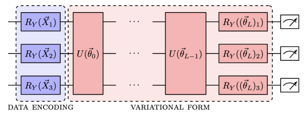
A Born machine represents a probability distribution as a quantum pure state and can generate samples via projective measurements. The Born machine outputs binary strings, which can be interpreted as a sample from the generated discrete probability distribution. Similar to a classification task, the target distribution is discretized into bins, which are associated with different binary strings of size . The quantum state can take the form of a quantum circuit Liu and Wang (2018) or a tensor network Wall et al. (2021), acting on some initial state, e.g., . Delgado and Hamilton (2022) numerically demonstrated that the initial state has only a negligible impact on the training, reason why this simple, physic-independent state is chosen. This paper considers quantum circuit Born machines, where the quantum circuit is constructed, for convenience, using repetitions of basic layers , where = is the set of all parameters. is a vector of trainable parameters for the specific layer which needs to be trained to match all amplitudes for the desired -qubit registers to find the corresponding state. These building blocks are chosen as a hardware-efficient ansatz Kandala et al. (2017), which can be run on current quantum chips with minimal overhead. An example constructed with and single-qubit rotations, where , are trainable parameters, and controlled NOT (CNOT) interaction between two qubits with linear connectivity is shown in Fig. 1. Here, () correspond to Pauli matrices
| (1) |
| (2) |
| (3) |
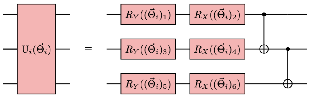
A rotation is always added before the measurements, which can be interpreted as optimizing the observable which is measured. Thus, the final unitary can be written as
| (4) | ||||
| (5) | ||||
| (6) |
where is a rotation of the th qubit around the axis with angle Nielsen and Chuang (2010) and CXk,j is a CNOT Nielsen and Chuang (2010) gate between qubits and .
III.2 Correlated features
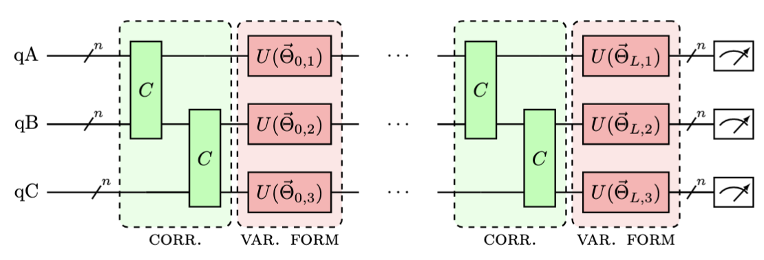
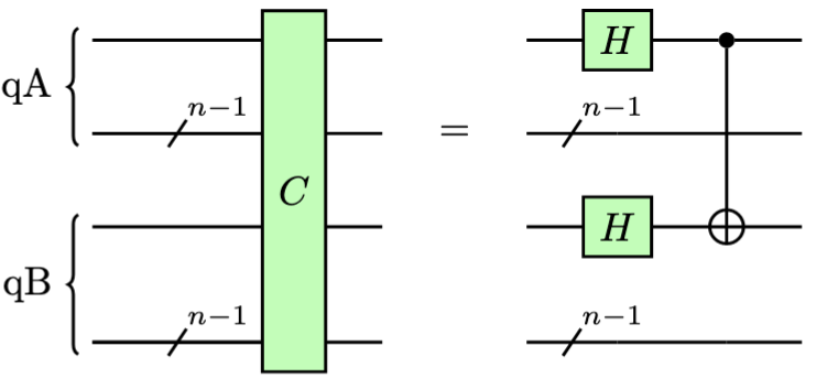
A simple way to extend the above-defined QCBM to generate correlated features is to use different registers (, , , etc) for each of them, as proposed in Ref. Zhu et al. (2021). We will therefore associate each feature with a quantum register of size , where the total number of qubits needed is . In this scenario, a fixed unitary entangles the registers while local operators learn the individual distributions, as shown in Fig. 2. The index refers to the layer, and refers to the register. While the local operators are trainable, the correlation gates do not contain any free parameters. This ensures that the number of parameters is kept to a minimum, considering that rotations are already included in the local operators. The operator is built with the following two-qubit block
| (7) |
which is used to entangle the th qubit of the and register. Here, refers to the Hadamard gate Nielsen and Chuang (2010). We consider different variations of this setup:
-
(1)
We vary the registers are entangled together, e.g. in a linear way, where each register is connected to the next one, or in a full way, where every register is connected to all the others.
-
(2)
We vary the number of qubits in each register which are acted upon, e.g., only the first pair (denoted by ), or all of them (, denoted by äll”). More precisely, the qubit is connected to the one for
-
(3)
Finally, we can choose the block to be
(8) which constructs a Bell state, when two registers are involved or,
(9) which constructs a Greenberger-Horne-Zeilinger state when there are three registers. This choice will be denoted by the label ”Bell”.
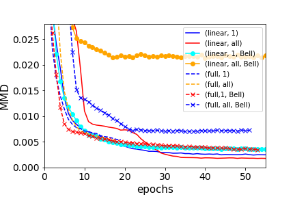
This gives eight possibilities in total, and they were all tested for the considered use case. A comparison will be shown in Sec. V.3. However, we can already mention that an easier choice, such as (linear, 1) or (linear, 1, Bell), with a reduced connectivity and number of gates usually leads to higher performance, in terms of both the marginal distribution and correlations. Moreover, while the more expensive option (linear, all) achieves a smaller loss on the simulator, it failed on the hardware since the execution time exceeded the coherence time of the device, producing uniform distributions from maximally mixed states. We therefore advocate for the use of the minimal (linear, 1) block, which can be constructed using the circuit depicted in Fig. 3.
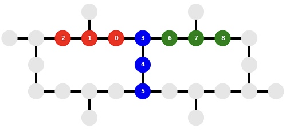
Moreover, it is possible, using the circuit in Fig. 1 for , for all and , to map the multivariate Born machine from Fig. 2, with the (linear, 1) choice to an IBM Quantum chip without using any SWAP gates. This is due to the linear connectivity of all the components and the T topology of the device. Fig. 4 shows a possible way to do so onto a 27-qubit architecture using three registers ( in red, in blue, and in green) with qubits each. The elimination of SWAP gates diminishes the number of errors made on the quantum devices by reducing the number of two-qubit gates and depth.
III.3 Conditional Born machine
Conditional generative models, such as conditional generative adversarial networks Mirza and Osindero (2014) produce samples according to some conditions . This task is more challenging since has to be captured, instead of only , where is the probability of event happening. The flexibility of conditional generative models compared to MC simulations is advantageous in terms of the computational and time resources needed to generate complex events. For instance, in the MC simulations used in this work, the initial energy of the incoming muon has to be fixed, while it is variable in ML-based techniques. This is a strong argument in favor of machine learning, both classical and quantum, for data generation in HEP. Hence, while the MC computations have to be performed for all the different values of the conditioning variable, machine learning models can learn from a reduced training set, and interpolate, or even extrapolate, considerably reducing the time consumption needed for MC simulations.
Condition in MFC events is the energy of the incoming muon. Different experimental values for are considered, ranging from 50 to 200 GeV in steps of 25 GeV. The conditional QCBM’s goal is to generate the correct distributions when given access to the incoming muon’s energy. In practice, is first scaled between [0,1], is transformed with the function arcsine, as used in Kiss et al. (2022), and is then encoded into the QCBM via repeated rotations on all qubits, as shown in Fig. 5.
The preprocessing ensures that the data are in the right range to be interpreted as an angle. Overall, the model consists of a feature map which encodes the data and trainable gates that learn the probability distribution, and can be written as
| (10) |
with as in Eq. 4, being the data-encoding feature map
| (11) |
and
| (12) |
Here, minmax scales the data set between the values and .
IV Training Strategy
IV.1 Optimization
The QCBM is trained using a two-sample test Gretton et al. (2012), with a Gaussian kernel
| (13) |
by comparing the distance between two samples and in the kernel feature space. Concretely, the maximum mean discrepancy (MMD) Gretton et al. (2012) loss function
| (14) |
is used, with bandwidth
| (15) |
In this way, the differences of all the moments between the target and model probability distributions are efficiently compared at different scales. The advantages of the MMD include its metric properties and the training stability it provides, making it a suitable option in the NISQ era.
The gradient can be computed Liu and Wang (2018) using the parameter-shift rule Schuld et al. (2019) as
| (16) |
where are QCBMs with parameters with being the th unit basis vector in the parameter space, i.e. .
Alternatively, the simultaneous perturbation stochastic approximation (SPSA) Spall (1998) algorithm is also considered to optimize the QCBM in a gradient-free fashion. SPSA efficiently approximates the gradient with two sampling steps by perturbing the parameters in all directions simultaneously. While the convergence is slower than using the exact gradient, fewer circuit evaluations are needed for each epoch. Moreover, the stochastic nature of SPSA makes it more resilient to hardware and statistical noise. It was observed during the simulations that the gradient-based algorithm outperforms SPSA, as SPSA sometimes gets trapped in local minima. However the gradient-based algorithm is more resource intensive than SPSA, and in this regime, SPSA is often preferred as it is better suited for quantum hardware.
Therefore, a mixed training scheme is used, where the models are first trained on (noisy) simulators using the adaptive moment estimator (ADAM) optimizer Kingma and Ba (2015) and then fine-tuned for a few epochs on quantum hardware using SPSA. A readout-error-mitigation scheme Nation et al. (2021) is used on the measurements. Details about the implementation, training, and resources can be found in the Appendix.
IV.2 Classical baseline
Classical generative models trained using the MMD loss function (GMMD models) Li et al. (2015); Dziugaite et al. (2015) are used as a baseline. They are trained on continuous data since the performance is usually higher than for discrete samples. The considered model is a simple fully connected neural network with only a few thousand parameters. It is highly probable that higher-performing models can be designed with some care. For instance, Ramazyan et al. (2022) shows a solution to the same problem using GAN. The goal of the classical baseline at this stage is to give an indication of the current level of deployability of quantum machine learning models and not to predict quantum advantage.
V Results
V.1 Experimental device
The quantum devices (IBMQ Montreal and IBMQ Mumbai Jurcevic et al. (2021)) used in this work consist of two 27-fixed-frequency transmon qubits, with fundamental transition frequencies of approximately 5 GHz and anharmonicities of MHz. Their topology is displayed in Fig. 4. Microwave pulses are used for single-qubit gates and cross-resonance interaction Chow et al. (2011) is used for two-qubit gates. The experiments took place over 3 hours each, without intermediate calibration. The median qubit lifetime of the qubits are 121 and 129 , the median coherence time are 90 and 135 and the median readout errors are 0.029 and 0.021 for the two devices, respectively. The qubits, which are used in the experiments, are chosen such that the total CNOT and readout error are minimized. The CNOT error varies between 0.006 and 0.02, depending on the specific connection.
V.2 One dimensional distribution
As a first demonstration, the QCBM is trained on a one-dimensional distribution: the energy of the outgoing muon discretized on bins. The QCBM is built with one repetition of and gates on all qubits and interaction on qubit and , using a full entanglement scheme. The unitary can thus be written as
| (17) | ||||
| (18) | ||||
| (19) |
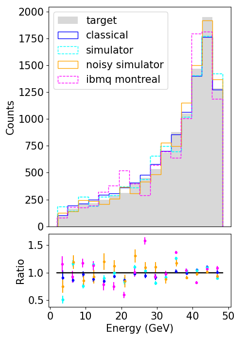
and has 18 parameters. This particular structure has been found to be best suited for the current situation via trial and error. In particular, empirical evidence suggests that this circuit is better suited than the one proposed in Fig. 1. The small number of two-qubit gates enables the use of real quantum hardware without severe complications due to the noise. Results obtained with an ideal simulator, noisy simulator, superconducting circuits (IBMQ Montreal) and classical GMMD are shown in Fig. 6. The histograms display the number of generated events and the ratios with the data set as a function of energy (GeV), with error bars corresponding to one standard deviation from 10 sampling processes.
The GMMD is chosen to be a neural network with four hidden layers of size , each with a sigmoid activation function, and a latent space of dimension 15.
The total variance (TV) with sample set ,
| (20) |
is used as a comparison metric and results are shown in Table 1.
| Backend | TV |
|---|---|
| Simulator | 0.055 |
| Noisy simulator | 0.043 |
| IBMQ Montreal | 0.074 |
| GMMD | 0.028 |
Although slightly outperformed by the GMMD, the QCBM can still be competitive even with its small number of parameters. The noise does not negatively contribute to the performance, as emphasized by the noisy simulations and quantum hardware results.
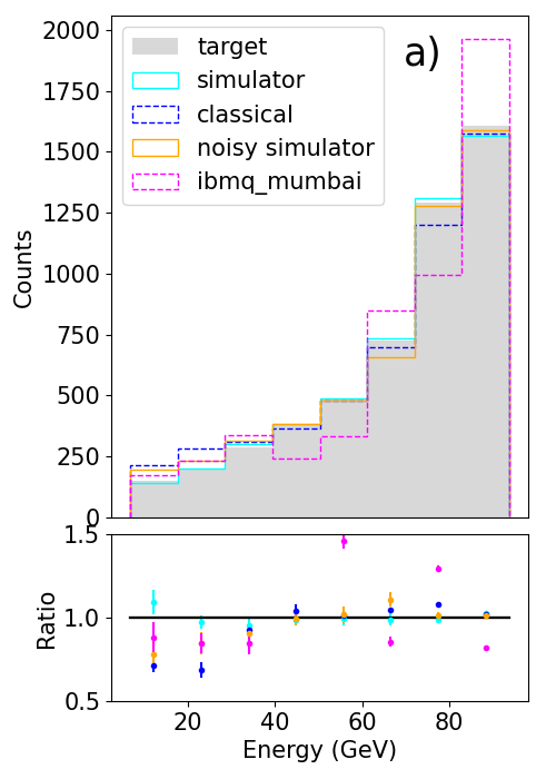
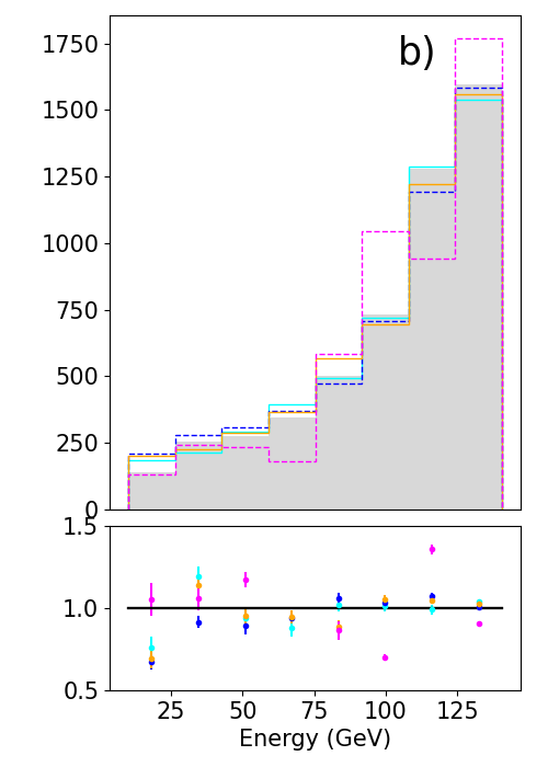
V.3 Multivariate distribution
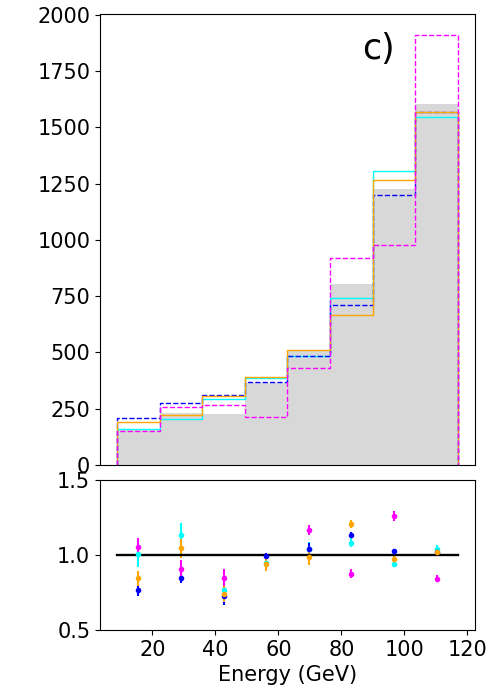
As a next step, we consider a multivariate distribution, namely, the energy, transverse momentum, and pseudorapidity of the outgoing muon with an incoming energy of 125 GeV, using bins. The QCBM is designed with four repetitions of entangling and a local block, as seen in Fig. 2. The former creates an entangling state, while the latter consists of and CNOT interaction with linear connectivity. The model therefore has parameters. We first assess the performance of the different choices for the correlation block described in Sec. III.2 by showing the validation MMD loss values during the training in Fig. 7. We observe that the (linear, 1) and (linear, all) blocks perform similarly and are the best choices for the present task. It is not surprising that the best results are obtained with the long-range interaction provided by (linear, all), as this outcome was also reported in Brian Coyle et al. (2020); Zhu et al. (2021). However, the performance obtained on the quantum hardware is improved by using the (linear, 1) block since it contains fewer CNOT gates. We will therefore choose this architecture for the rest of the paper.
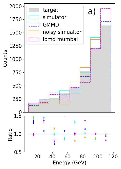
The results for the simulator, noisy simulator, IBMQ Mumbai, and GMMD are shown in Fig. 8 and the total variance for the marginal distributions are presented in Table 2. The GMMD is constructed similarly to that above but with three hidden layers of size . Even if the GMMD achieves the best accuracy, the QCBM is still competitive despite its small number of learned parameters or the presence of noise.
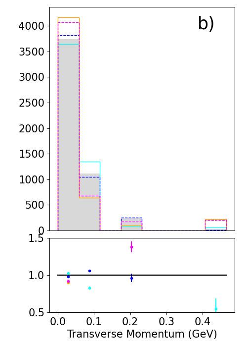
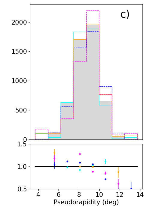
| Backend | |||
|---|---|---|---|
| Simulator | 0.055 | 0.05 | 0.052 |
| Noisy simulator | 0.075 | 0.12 | 0.06 |
| IBMQ Mumbai | 0.078 | 0.097 | 0.13 |
| GMMD | 0.036 | 0.017 | 0.063 |
An important factor for the performance of generative models is their ability to learn the correlations between the variables, which is not reflected in the total variance. To this point, the correlations in the target dataset are compared to those in the generated datasets. The correlation matrices are computed with the Pearson product-moment methods
| (21) |
where is the covariance matrix. The correlations in the target dataset (ground truth) are shown in Table 3 and those for the generated samples are in Table 4.
| \cellcolor[HTML]C0C0C0- | 0.43 | 0.89 | |
| 0.43 | \cellcolor[HTML]C0C0C0- | 0.61 | |
| 0.89 | 0.61 | \cellcolor[HTML]C0C0C0 - |
| sim | noisy | IBMQ | GMMD | sim. | noisy | IBMQ | GMMD | sim. | noisy | IBMQ | GMMD | ||
|---|---|---|---|---|---|---|---|---|---|---|---|---|---|
| \cellcolor[HTML]C0C0C0- | \cellcolor[HTML]38FFF80.6 | \cellcolor[HTML]FFC7020.3 | \cellcolor[HTML]EC71FE0.29 | \cellcolor[HTML]3531FF 0.44 | \cellcolor[HTML]38FFF80.9 | \cellcolor[HTML]FFCB2F0.87 | \cellcolor[HTML]EC71FE0.88 | \cellcolor[HTML]3531FF 0.91 | |||||
| \cellcolor[HTML]38FFF80.6 | \cellcolor[HTML]FFC7020.3 | \cellcolor[HTML]EC71FE0.29 | \cellcolor[HTML]3531FF 0.44 | \cellcolor[HTML]C0C0C0- | \cellcolor[HTML]38FFF80.79 | \cellcolor[HTML]FFCB2F0.58 | \cellcolor[HTML]EC71FE0.6 | \cellcolor[HTML]3531FF 0.61 | |||||
| \cellcolor[HTML]38FFF80.9 | \cellcolor[HTML]FFC7020.87 | \cellcolor[HTML]EC71FE0.88 | \cellcolor[HTML]3531FF 0.91 | \cellcolor[HTML]38FFF80.79 | \cellcolor[HTML]FFC7020.58 | \cellcolor[HTML]EC71FE0.6 | \cellcolor[HTML]3531FF 0.61 | \cellcolor[HTML]C0C0C0- | |||||
We observe that the QCBMs trained on the different backends are able to capture the correct correlations, even if the classical GMMD is better. It is noteworthy that the samples generated by the quantum chip are closer to the ground truth than the simulated ones, suggesting that generative modeling is a promising task for NISQ devices.
V.4 Conditional distribution
Finally, we consider conditional QCBM for the generation of MC events conditioned on the initial muon’s energy, which is encoded in the QCBM via parametrized-rotations. The QCBM, as outlined in Fig. 5 contains four repetitions of , with and rotations (with different parameters) and CNOT interaction in a linear fashion as depicted in Fig. 1, while the GMMD has two hidden layers of size . The thus QCBM contains 27 trainable parameters. The training is performed on the whole dataset except at 125 GeV, which is left to test the interpolation capabilities of the models. Results are shown in Fig. 9, and the values of the total variance are reported in Table 5. All models achieve good performance for the interpolation. The results on the quantum hardware could be slightly improved for some histogram binned values. However, the performance is similar on training and testing energy bins, suggesting that the QCBM can interpolate but is strongly affected by the noise.
| Backend | |||
|---|---|---|---|
| Simulator | 0.033 | 0.016 | 0.033 |
| Noisy simulator | 0.067 | 0.046 | 0.035 |
| IBMQ Mumbai | 0.15 | 0.13 | 0.094 |
| GMMD | 0.016 | 0.032 | 0.034 |
VI Discussion
The results presented in the Sec. V suggest that QCBMs can reproduce the marginal distribution, as well as the correlations, from MC simulations. Even if a higher performance can easily be obtained with classical neural networks, it is important to underline that QCBMs generally operate with very few parameters for similar performance. This suggests that QCBMs are more expressive than classical neural networks, as outlined by Abbas et al. (2021), and outperform them in the under-parametrized regime. It remains an open question whether QCBMs enjoy a higher performance in the overparameterized regime, as is the case for classical models Nakkiran et al. (2021). We note that this question was already explored for quantum neural networks by Larocca et al. (2021).
Moreover, the presence of noise does not seem to be an obstacle to the training of QCBMs. It is noteworthy that the results obtained on quantum hardware are close to that obtained on the simulator, which suggests sufficient device quality for this task and an ability to deal with incoherent noise. The hardware results are slightly worse in the conditional case which can be explained by the reduced number of epochs performed on the quantum hardware. The loop over the training energy bins increases the resources needed for one epoch, and thus reduces the number of epochs performed.
These observations suggest that the noise is assimilated during the training, underlining the importance of using actual quantum hardware. This supports the findings of Borras et al. (2022), which empirically found that quantum generative adversarial networks can be efficiently trained on quantum hardware if the readout noise is smaller than 0.1. Thus, QCBMs seem to be an appealing application for NISQ devices.
Barren plateaus (BP) are large portions of the training landscape where the loss function’s gradient variance vanishes. As shown in McClean et al. (2018), BPs appear exponentially fast in the depth and number of qubits for generic quantum circuits, which makes the training of large-scale quantum variational algorithms generally difficult. Solutions to this issue, such as quantum convolutional neural networks Cong et al. (2019) and local loss functions Cerezo et al. (2021) are not applicable in this case since measurements on all qubits are needed.
However, BPs have not been observed in this work, and were not reported in similar studies Zhu et al. (2021); Delgado and Hamilton (2022) either. This can be explained to some extent by the relative shallowness of the circuits used. Nevertheless, difficulties are observed durings training on hardware and noisy simulators, which could be an effect of noise-induced BPs Wang et al. (2021b). A more significant number of epochs was needed to mitigate this effect. Increasing the number of qubits to five or six, for the one-dimensional case, causes the ratio between the generated and target samples for each bin to deteriorate, even if the loss function converged after a hundred epochs. The same problem appeared when increasing the number of features in the multivariate case and mixing multiple features with the conditioning. Since the gradient never vanished at the beginning of the training, BPs are probably not the most critical issue, on the other hand, the MMD may not be the most suitable loss function for large-scale QCBMs.
Alternative training strategies were proposed in Brian Coyle et al. (2020); Zoufal et al. (2019), with optimal transport and an adversarial training strategy, respectively. Hence, empirical evidence suggests that the strong theoretical properties of the MMD loss function are not met in practice, as outlined by some benchmarks Liu et al. (2015). Hence, the performances of GMMD and GAN are similar for simple problems but the latter is superior for complex tasks. Li et al. (2017) proposed an adversarial strategy to optimize the kernel as an efficient way to improve the performance of GMMD models.
VII Conclusion
The present paper presented the application and further development of a quantum circuit Born machine to generate Monte Carlo events in HEP, specifically muon force carriers. An efficient way to generate multivariate distributions, requiring only linear connectivity and thus being suitable for NISQ devices, was proposed. Additionally, the present paper took a step towards generating conditional probability distributions with quantum circuit Born machines. Numerical evidence demonstrated that QCBMs can efficiently generate joint and conditional distributions with the correct correlations. Finally, the experiments were run successfully on quantum hardware, hinting that QML algorithms can mitigate the effect of the noise during the training. Quantum generative models are consequently appealing for NISQ devices since they can manage noisy qubits without the need of for expensive error-mitigation techniques. QCBMs also have the advantage of needing a small number of parameters while still being competitive.
While having strong potential in generative modeling, QCBMs still need some improvement to handle a more refined binning and multivariate distribution of higher dimensions. Additionally, it would be interesting to consider conditional distributions which are more sensitive to the conditioning variable, and they will be the focus of future work.
Acknowledgement
The authors thank S. Y. Chang, D. Pasquali, T. Ramazyan, and F. Rehm for valuable and stimulating discussions about the present paper.
This work was supported by the CERN Quantum Technology Initiative. Simulations were performed on the University of Geneva’s Yggdrasil HPC cluster. Access to the IBM Quantum Services was obtained through the IBM Quantum Hub at CERN. The views expressed are those of the authors and do not reflect the official policy or position of IBM or the IBM Q team.
Literatur
- Shor (1997) Peter W. Shor, “Polynomial-time algorithms for prime factorization and discrete logarithms on a quantum computer,” SIAM Journal on Computing 26, 1484–1509 (1997).
- Kitaev (1996) Alexei Y. Kitaev, “Quantum measurements and the abelian stabilizer problem,” Electron. Colloquium Comput. Complex. (1996).
- Preskill (2018) John Preskill, “Quantum Computing in the NISQ era and beyond,” Quantum 2, 79 (2018).
- Biamonte et al. (2017) Jacob Biamonte, Peter Wittek, Nicola Pancotti, Patrick Rebentrost, Nathan Wiebe, and Seth Lloyd, “Quantum machine learning,” Nature 549, 195–202 (2017).
- McClean et al. (2016) Jarrod R McClean, Jonathan Romero, Ryan Babbush, and Alán Aspuru-Guzik, “The theory of variational hybrid quantum-classical algorithms,” New Journal of Physics 18, 023023 (2016).
- Mitarai et al. (2018) K. Mitarai, M. Negoro, M. Kitagawa, and K. Fujii, “Quantum circuit learning,” Phys. Rev. A 98, 032309 (2018).
- Kiss et al. (2022) Oriel Kiss, Francesco Tacchino, Sofia Vallecorsa, and Ivano Tavernelli, “Quantum neural networks force field generation,” Mach. Learn.: Sci. Technol. 3 (2022), https://doi.org/10.1088/2632-2153/ac7d3c.
- Schuld and Killoran (2019) Maria Schuld and Nathan Killoran, “Quantum machine learning in feature hilbert spaces,” Phys. Rev. Lett. 122, 040504 (2019).
- Cong et al. (2019) Iris Cong, Soonwon Choi, and Mikhail D. Lukin, “Quantum convolutional neural networks,” Nat. Phys. 15, 1273–178 (2019).
- Havlíček et al. (2019) V. Havlíček, A. D. Córcoles, K. Temme, A. W. Harrow, A. Kandala, J. M. Chow, and J. M. Gambetta, “Supervised learning with quantum-enhanced feature spaces,” Nature 567, 209–212 (2019).
- Zoufal et al. (2019) Christa Zoufal, Aurélien Lucchi, and Stefan Woerner, “Quantum generative adversarial networks for learning and loading random distributions,” npj Quantum Inf 5 (2019), https://doi.org/10.1038/s41534-019-0223-2.
- Brian Coyle et al. (2020) Daniel Mills Brian Coyle, Vincent Danos, and Elham Kashefi, “The born supremacy: quantum advantage and training of an ising born machine,” npj Quantum Inf 6, 60 (2020).
- Liu and Wang (2018) Jin-Guo Liu and Lei Wang, “Differentiable learning of quantum circuit born machines,” Phys. Rev. A 98, 062324 (2018).
- Schuld et al. (2015) Maria Schuld, Ilya Sinayskiy, and Francesco Petruccione, “An introduction to quantum machine learning,” Contemporary Physics 56, 172–185 (2015), https://doi.org/10.1080/00107514.2014.964942 .
- Kandala et al. (2017) Abhinav Kandala, Antonio Mezzacapo, Kristan Temme, Maika Takita, Markus Brink, Jerry M. Chow, and Jay M. Gambetta, “Hardware-efficient variational quantum eigensolver for small molecules and quantum magnets,” Nature 549, 242–246 (2017).
- Romero et al. (2019) Jonathan Romero, Ryan Babbush, Jarrod R McClean, Cornelius Hempel, Peter J Love, and Alán Aspuru-Guzik, “Strategies for quantum computing molecular energies using the unitary coupled cluster ansatz,” Quantum Sci. Technol. 4, 014008 (2019).
- Crippa et al. (2021) Luca Crippa, Francesco Tacchino, Mario Chizzini, Antonello Aita, Michele Grossi, Alessandro Chiesa, Paolo Santini, Ivano Tavernelli, and Stefano Carretta, “Simulating static and dynamic properties of magnetic molecules with prototype quantum computers,” Magnetochemistry 7 (2021), 10.3390/magnetochemistry7080117.
- Goodfellow et al. (2014) Ian Goodfellow, Jean Pouget-Abadie, Mehdi Mirza, Bing Xu, David Warde-Farley, Sherjil Ozair, Aaron Courville, and Yoshua Bengio, “Generative adversarial nets,” Advances in Neural Information Processing Systems, 27 (2014).
- Kingma and Welling (2014) Diederik P. Kingma and Max Welling, “Auto-encoding variational bayes,” Conference proceedings: paper accepted to the International Conference on Learning Representations (ICLR) 2014 (2014), 10.48550/ARXIV.1312.6114.
- Wang et al. (2021a) Zhengwei Wang, Qi She, and Tomás E. Ward, “Generative adversarial networks in computer vision: A survey and taxonomy,” ACM Comput. Surv. 54 (2021a), 10.1145/3439723.
- Carleo et al. (2019) Giuseppe Carleo, Ignacio Cirac, Kyle Cranmer, Laurent Daudet, Maria Schuld, Naftali Tishby, Leslie Vogt-Maranto, and Lenka Zdeborová, “Machine learning and the physical sciences,” Rev. Mod. Phys. 91, 045002 (2019).
- Vallecorsa (2018) Sofia Vallecorsa, “Generative models for fast simulation,” Journal of Physics: Conference Series 1085 (2018).
- Paganini et al. (2018) Michela Paganini, Luke de Oliveira, and Benjamin Nachman, “Calogan: Simulating 3d high energy particle showers in multilayer electromagnetic calorimeters with generative adversarial networks,” Phys. Rev. D 97, 014021 (2018).
- Maevskiy et al. (2020) A Maevskiy, D Derkach, N Kazeev, A Ustyuzhanin, M Artemev, and L Anderlini, “Fast data-driven simulation of cherenkov detectors using generative adversarial networks,” Journal of Physics: Conference Series 1525, 012097 (2020).
- Agliardi et al. (2022) Gabriele Agliardi, Michele Grossi, Mathieu Pellen, and Enrico Prati, “Quantum integration of elementary particle processes,” Physics Letters B 832, 137228 (2022).
- Agostinelli et al. (2003) S. Agostinelli et al. (GEANT4), “GEANT4–a simulation toolkit,” Nucl. Instrum. Meth. A 506, 250–303 (2003).
- Stelzer and Long (1994) T. Stelzer and W. F. Long, “Automatic generation of tree level helicity amplitudes,” Comput. Phys. Commun 84, 357–371 (1994).
- collaboration et al. (2018) The CMS collaboration, Sirunyan A.M., Tumasyan A., and et al., “Measurement of the cross section for top quark pair production in association with a w or z boson in proton-proton collisions at tev,” J. High Energ. Phys. 2018 (2018), https://doi.org/10.1007/JHEP08(2018)011.
- Benedetti1 et al. (2019) Marcello Benedetti1, Erika Lloyd, Stefan Sack, and Mattia Fiorentini, “Parameterized quantum circuits as machine learning models,” Quantum Science and Technology 4 (2019), 10.1088/2058-9565/ab4eb5.
- Chang et al. (2021) Su Yeon Chang, Steven Herbert, Sofia Vallecorsa, Elías F. Combarro, and Ross Duncan, “Dual-parameterized quantum circuit gan model in high energy physics,” EPJ Web Conf. 251 (2021), https://doi.org/10.1051/epjconf/202125103050.
- Benedetti et al. (2021) Marcello Benedetti, Brian Coyle, Mattia Fiorentini, Michael Lubasch, and Matthias Rosenkranz, “Variational inference with a quantum computer,” Phys. Rev. Applied 16, 044057 (2021).
- Čepaitė et al. (2022) Ieva Čepaitė, Brian Coyle, and Elham Kashefi, “A continuous variable born machine,” Quantum Mach. Intell. 4, 6 (2022).
- Romero and Aspuru-Guzik (2019) Jonathan Romero and Alan Aspuru-Guzik, “Variational quantum generators: Generative adversarial quantum machine learning for continuous distributions,” ArXiv e-prints (2019), arXiv:1901.00848 [quant-ph] .
- Bravo-Prieto et al. (2022) Carlos Bravo-Prieto, Julien Baglio, Marco Cè, Anthony Francis, Dorota M. Grabowska, and Stefano Carrazza, “Style-based quantum generative adversarial networks for Monte Carlo events,” Quantum 6, 777 (2022).
- Zoufal et al. (2021) Christa Zoufal, Aurélien Lucchi, and Stefan Woerner, “Variational quantum boltzmann machines,” Quantum Machine Intelligence 3 (2021), https://doi.org/10.1007/s42484-020-00033-7.
- Alcazar et al. (2020) Javier Alcazar, Vicente Leyton-Ortega, and Alejandro Perdomo-Ortiz, “Classical versus quantum models in machine learning: insights from a finance application,” Machine Learning: Science and Technology 1, 035003 (2020).
- Zhu et al. (2021) Elton Yechao Zhu, Sonika Johri, Mert Esencan Dave Bacon, Jungsang Kim, Mark Muir, Nikhil Murgai, Jason Nguyen, Neal Pisenti, Adam Schouela, Ksenia Sosnova, and Ken Wright, “Generative quantum learning of joint probability distribution functions,” ArXiv e-prints (2021), arXiv:2109.06315 [quant-ph] .
- Delgado and Hamilton (2022) Andrea Delgado and Kathleen E. Hamilton, “Unsupervised quantum circuit learning in high energy physics,” ArXiv e-prints (2022), arXiv:2203.03578 [quant-ph] .
- Galon et al. (2020) Iftah Galon, Enrique Kajamovitz, David Shih, Yotam Soreq, and Shlomit Tarem, “Searching for muonic forces with the atlas detector,” Phys. Rev. D 101, 011701 (2020).
- Galon et al. (2022) Iftah Galon, Enrique Kajamovitz, David Shih, Yotam Soreq, and Shlomit Tarem, “Muonic force carriers,” (2022).
- In-Kwon and Johnson (2000) Yeo In-Kwon and Richard A. Johnson, “A new family of power transformations to improve normality or symmetry,” Biometrika 87, 954–59 (2000).
- Ramazyan et al. (2022) Tigran Ramazyan, Oriel Kiss, Michele Grossi, Enrique Kajomovitz, and Sofia Vallecorsa, “Generating muonic force carriers events with classical and quantum neural networks,” J. Phys.: Conf. Ser. (Submitted) (2022).
- Wall et al. (2021) Michael L. Wall, Matthew R. Abernathy, and Gregory Quiroz, “Generative machine learning with tensor networks: Benchmarks on near-term quantum computers,” Phys. Rev. Research 3, 023010 (2021).
- Nielsen and Chuang (2010) Michael A. Nielsen and Isaac L. Chuang, Quantum Computation and Quantum Information: 10th Anniversary Edition (Cambridge University Press, 2010).
- Mirza and Osindero (2014) Mehdi Mirza and Simon Osindero, “Conditional generative adversarial nets,” ArXiv e-prints (2014), arXiv:1411.1784 [cs.AI] .
- Schuld et al. (2021) Maria Schuld, Ryan Sweke, and Johannes Jakob Meyer, “Effect of data encoding on the expressive power of variational quantum-machine-learning models,” Phys. Rev. A 103, 032430 (2021).
- Gretton et al. (2012) Arthur Gretton, Karsten M. Borgwardt, Malte J. Rasch, Bernhard Schölkopf, and Alexander Smola, “A kernel two-sample test,” J. Mach. Learn. Res. 13, 723–773 (2012).
- Schuld et al. (2019) Maria Schuld, Ville Bergholm, Christian Gogolin, Josh Izaac, and Nathan Killoran, “Evaluating analytic gradients on quantum hardware,” Phys. Rev. A 99, 032331 (2019).
- Spall (1998) J.C. Spall, “Implementation of the simultaneous perturbation algorithm for stochastic optimization,” IEEE Transactions on Aerospace and Electronic Systems 34, 817–823 (1998).
- Kingma and Ba (2015) Diederik P. Kingma and Jimmy Ba, “Adam: A method for stochastic optimization,” in 3rd International Conference on Learning Representations, ICLR 2015, San Diego, CA, USA, May 7-9, 2015, Conference Track Proceedings, edited by Yoshua Bengio and Yann LeCun (2015).
- Nation et al. (2021) Paul D. Nation, Hwajung Kang, Neereja Sundaresan, and Jay M. Gambetta, “Scalable mitigation of measurement errors on quantum computers,” PRX Quantum 2, 040326 (2021).
- Li et al. (2015) Yujia Li, Kevin Swersky, and Rich Zemel, “Generative moment matching networks,” Proceedings of the 32nd International Conference on Machine Learning, Proceedings of Machine Learning Research, 37, 1718–1727 (2015).
- Dziugaite et al. (2015) Gintare Karolina Dziugaite, Daniel M. Roy, and Zoubin Ghahramani, “Training generative neural networks via maximum mean discrepancy optimization,” in Proceedings of the Thirty-First Conference on Uncertainty in Artificial Intelligence, UAI’15 (AUAI Press, Arlington, Virginia, USA, 2015) p. 258–267.
- Jurcevic et al. (2021) Petar Jurcevic, Ali Javadi-Abhari, Lev S Bishop, Isaac Lauer, Daniela F Bogorin, Markus Brink, Lauren Capelluto, Oktay Günlük, Toshinari Itoko, Naoki Kanazawa, Abhinav Kandala, George A Keefe, Kevin Krsulich, William Landers, Eric P Lewandowski, Douglas T McClure, Giacomo Nannicini, Adinath Narasgond, Hasan M Nayfeh, Emily Pritchett, Mary Beth Rothwell, Srikanth Srinivasan, Neereja Sundaresan, Cindy Wang, Ken X Wei, Christopher J Wood, Jeng-Bang Yau, Eric J Zhang, Oliver E Dial, Jerry M Chow, and Jay M Gambetta, “Demonstration of quantum volume 64 on a superconducting quantum computing system,” Quantum Science and Technology 6, 025020 (2021).
- Chow et al. (2011) Jerry M. Chow, A. D. Córcoles, Jay M. Gambetta, Chad Rigetti, B. R. Johnson, John A. Smolin, J. R. Rozen, George A. Keefe, Mary B. Rothwell, Mark B. Ketchen, and M. Steffen, “Simple all-microwave entangling gate for fixed-frequency superconducting qubits,” Phys. Rev. Lett. 107, 080502 (2011).
- Abbas et al. (2021) Amira Abbas, David Sutter, Christa Zoufal, Aurelien Lucchi, Alessio Figalli, and Stefan Woerner, “The power of quantum neural networks,” Nature Computational Science 1, 403–409 (2021).
- Nakkiran et al. (2021) Preetum Nakkiran, Gal Kaplun, Yamini Bansal, Tristan Yang, Boaz Barak, and Ilya Sutskever, “Deep double descent: where bigger models and more data hurt,” Journal of Statistical Mechanics: Theory and Experiment 2021, 124003 (2021).
- Larocca et al. (2021) Martin Larocca, Nathan Ju, Diego García-Martín, Patrick J. Coles, and M. Cerezo, “Theory of overparametrization in quantum neural networks,” ArXiv e-prints (2021), arXiv:2109.11676 [quant-ph] .
- Borras et al. (2022) Kerstin Borras, Su Yeon Chang, Lena Funcke, Michele Grossi, Tobias Hartung, Karl Jansen, Dirk Kruecker, Stefan Kühn, Florian Rehm, Cenk Tüysüz, and Sofia Vallecorsa, “Impact of quantum noise on the training of quantum generative adversarial networks,” ArXiv e-prints (2022), arXiv:2203.01007 [quant-ph] .
- McClean et al. (2018) Jarrod R. McClean, Sergio Boixo, Vadim N. Smelyanskiy, Ryan Babbush, and Hartmut Neven, “Barren plateaus in quantum neural network training landscapes,” Nature Communications 9 (2018), https://doi.org/10.1038/s41467-018-07090-4.
- Cerezo et al. (2021) M. Cerezo, Akira Sone, Tyler Volkoff, Lukasz Cincio, and Patrick J. Coles, “Cost function dependent barren plateaus in shallow parametrized quantum circuits,” Nat. Commun. 12 (2021), https://doi.org/10.1038/s41467-021-21728-w.
- Wang et al. (2021b) Samson Wang, Enrico Fontana, M. Cerezo, Kunal Sharma, Akira Sone, Lukasz Cincio, and Patrick J. Coles, “Noise-induced barren plateaus in variational quantum algorithms,” Nat Commun 12, 6961 (2021b).
- Liu et al. (2015) Z. Liu, P. Luo, X. Wang, and X. Tang, “Deep learning face attributes in the wild,” in 2015 IEEE International Conference on Computer Vision (ICCV) (IEEE Computer Society, Los Alamitos, CA, USA, 2015) pp. 3730–3738.
- Li et al. (2017) Chun-Liang Li, Wei-Cheng Chang, Yu Cheng, Yiming Yang, and Barnabas Poczos, “Mmd gan: Towards deeper understanding of moment matching network,” in Advances in Neural Information Processing Systems, Vol. 30, edited by I. Guyon, U. Von Luxburg, S. Bengio, H. Wallach, R. Fergus, S. Vishwanathan, and R. Garnett (Curran Associates, Inc., 2017).
- Bergholm (2018) Ville et al. Bergholm, “Pennylane: Automatic differentiation of hybrid quantum-classical computations,” ArXiv e-prints (2018), arXiv:1811.04968 [quant-ph] .
- Bradbury et al. (2018) James Bradbury, Roy Frostig, Peter Hawkins, Matthew James Johnson, Chris Leary, Dougal Maclaurin, George Necula, Adam Paszke, Jake VanderPlas, Skye Wanderman-Milne, and Qiao Zhang, “JAX: composable transformations of Python+NumPy programs,” (2018).
- et al. (2022) Matthew Treinish et al., “Qiskit/qiskit: Qiskit 0.37.1,” (2022).
Anhang A Implementation
The noiseless simulations are performed with PENNYLANE Bergholm (2018) powered by JAX Bradbury et al. (2018), which enables an efficient gradient computation via vectorization and just-in-time compilation. The noisy simulations are performed using a fake backend tuned to the real quantum hardware, provided by QISKIT et al. (2022). The fake backend has the same characteristics on average as the real backend described in Sec. V.1. The training is performed in batches composed of 512 events each, and one epoch is composed of 10 batches. The learning rate is initially set to 0.01 and is halved every 20 epochs. The resources needed to produce the presented results are presented in Table 6, which shows the number of parameters, the time needed for a forward pass and a backward pass, and the number of epochs until convergence for all the quantum models trained on the simulator. Each epoch is composed of 10 batches, except the conditional model which has 10 batches per training energy bin (i.e., six). Each batch contained 512 samples. Simulations were run on a single CPU on the University of Geneva’s Yggdrasil HPC cluster.
| Model | Param. | Forward | Backward | Epochs |
|---|---|---|---|---|
| pass (s) | pass (s) | |||
| One-dimensional | 18 | 1.2 | 3.9 | 70 |
| Multivariate | 45 | 1.9 | 9.4 | 100 |
| Conditional | 27 | 1.5 | 4.5 | 30 |