Quasinormal modes of Kerr-like black bounce spacetime

Abstract

The quasinormal modes of the Kerr-like black bounce spacetime under the scalar field perturbations are studied. We derive the effective potential of scalar perturbation in Kerr-like black bounce spacetime, and study the influence of Kerr-like black bounce spacetime parameters on quasinormal modes by using WKB method and Pöschl-Teller potential approximation. We find that Kerr-like black bounce spacetime has the analogous double-peaked potential as Schwarzschild-like black bounce spacetime, and mass of the scalar particle has a non-negligible effect on quasinormal modes of Kerr-like black bounce spacetime.

I Introduction

Since the first direct gravitational-wave (GW) detection by the Laser Interferometer Gravitational-Wave Observatory (LIGO) Scientific and Virgo Collaboration Abbott et al. (2016), and then first direct observation of a black hole and its shadow by the Event Horizon Telescope (EHT) Akiyama et al. (2019, 2022), we have an unique way to test strong gravity which has made possible new probing of modified gravity theories in the strong-field regime. The importance of emerging field of GW astronomy and physics provide opportunities these tests to the highly relativistic regime that characterizes merging BH binaries and also merging binary neutron stars Barack et al. (2019); Martinelli and Casas (2021); Chen et al. (2021); Berti et al. (2015); Çimdiker et al. (2021); Cardoso et al. (2016a); Barausse et al. (2020). Post-Newtonian (PN) formalism which is a perturbative approximation to General Relativity (GR) in weak-field, slow-motion situations breaks down (except in the early-inspiral phase). Signal of binary merger is occurred by three stages: the inspiral, merger, and ringdown. The last stage is in the form of a ringdown (a superposition of quasinormal modes (QNMs) vibrations of the merged remnant black holes, known as damped oscillations with characteristic resonant frequencies and damping times, which can provide important insight into the process and dynamics of astrophysical black holes Qian et al. (2022); Kuang and Wu (2017); Fernando (2016); Fernando and Correa (2012); Fernando (2004, 2009, 2008); Fernando and Clark (2014); Cardoso et al. (2016b); Cardoso and Pani (2017); Maggio et al. (2019); Konoplya and Zhidenko (2022); Konoplya et al. (2019a); Bronnikov and Konoplya (2020); Churilova et al. (2021).

Alternative theories of gravity are extension of the form of Einstein’s GR through various methods, has output of different field equations, hence different black hole solutions and cosmological models. Nowadays, alternative theories of gravity and their applications are a playground of physicist, provide a basis for the now-known understanding of physical phenomena of the universe Simpson and Visser (2021, 2022); Shankaranarayanan and Johnson (2022); Odintsov et al. (2022); Baker et al. (2021); Ferreira (2019); Pantig and Övgün (2022); Pantig et al. (2022); Kubiznak and Mann (2012); Gunasekaran et al. (2012); Kerner and Mann (2008); Akhmedov et al. (2006); Singleton and Wilburn (2011). The spectrum of known stationary black hole solutions in modified gravity theories has dramatically increased, sometimes in unexpected ways. The well-known stationary black hole solution is Kerr black hole solution according to black hole uniqueness theorems, it is the unique solution describing all rotating black holes in vacuum. Ongoing experiments like LIGO/VIRGO collaboration can give some possible constrains of deviations from the Kerr metric so that thrill of possibilities of this have accelerate an expressive proportion of studies in recent years to derive new methods for calculating QNMs, as well as focus largely on QNMs calculation of Kerr-like black holes beyond GR, which produced garden variety of Kerr black holes Daghigh and Green (2009, 2012); Daghigh et al. (2020); Zhidenko (2004, 2006); Konoplya and Zhidenko (2011); Chabab et al. (2017); Lepe and Saavedra (2005); González et al. (2017); Okyay and Övgün (2022); González et al. (2021); Panotopoulos and Rincón (2021, 2020, 2019); Rincón and Panotopoulos (2018); Övgün and Jusufi (2018); Övgün et al. (2018); Berti et al. (2009); Cardoso et al. (2009); Andersson and Howls (2004); Andersson (1997); Andersson and Onozawa (1996); Andersson and Linnæus (1992); Andersson (1995); Wang et al. (2002). Hence, in principle, no-hair theorem and GR can be tested using the QNMs.

In 2019, Simpson and M. Visser Simpson and Visser (2019), cleverly suggested a new way to merge a standard Schwarzschild black hole ($a=0$ and $m\neq 0$) with the wormhole spacetime ($a\geq 2m$) by simply introducing $a$ parameter, known as black-bounce spacetime. Recently, new version of the Simpson-Visser spacetime have been obtained in Lobo et al. (2021). Since then various physical analyses are done on the black-bounce spacetime. For instance, Churilova and Stuchlik have studied the QNMs using the WKB method with Padé expansion and the time-domain integration Churilova and Stuchlik (2020). Moreover, the influence of the black-bounce solution on the gravitational wave echoes signal in brane worlds has been studied by Bronnikov and Konoplya Bronnikov and Konoplya (2020). Then Bronnikov et al. have studied the general parametrization for spacetimes of spherically symmetric wormholes in an arbitrary metric theory of gravity, and have calculated its quasinormal modesBronnikov et al. (2021). Nascimento et al. have calculated the angular deflection of light, in the weak and strong field limit, in the black-bounce spacetime Nascimento et al. (2020). Moreover, Tsukamoto have also investigated strong gravitational lensing in the Simpson-Visser spacetime but in all the nonnegative parameters of $a$ and $m$ Tsukamoto (2021). Övgün has studied the weak deflection angle of black-bounce spacetime in dark matter medium using Gauss-Bonnet theorem Övgün (2020). Lima et al. have investigated absorption of massless scalar waves in the black-bounce spacetime Lima et al. (2020). Lobo et al. have constructed the spherically symmetric thin-shell traversable wormholes using black-bounce spacetimes Lobo et al. (2020). Mazza et al. have studied a special case of rotating black bounce space-time Mazza et al. (2021), and Franzin et al. studied the quasinormal modes of this space-time Franzin et al. (2022). Afterwards, Franzin et al. have constructed charged black-bounce spacetimesFranzin et al. (2021). Xu and Tang have constructed Kerr-like black-bounce space-time by using Newman-Janis algorithm Xu and Tang (2021). Guerrero et al. have analysed the light rings and shadows of black-bounce spacetime illuminated by a thin accretion disk Guerrero et al. (2021). Ou et al. have studied the time evolution of the field perturbations in the wormhole and black bounce backgrounds Ou et al. (2021). Tsukamoto have studied retrolensing by two photon spheres in a novel black-bounce spacetime Tsukamoto (2022).

One of the key motivations behind this paper is to study the characteristic “sound” of Kerr-like black-bounce space-time under scalar filed perturbation, i.e. the QNMs, whose real part represents the actual oscillation frequency after the perturbation, and the imaginary part represents the damp rate. This paper is organized as follows. In the next section we brief review of Kerr-like black-bounce space-time. Furthermore, we calculated the determinant of metric tensor and contravariant form of metric tensor. In Section III, the effective potential under scalar perturbations of the Kerr-like black bounce space-time is derived. In Section IV, we introduce the Pöschl-Teller potential approximation and semi-analytic WKB method for calculating quasinormal modes of the Kerr-like black bounce space-time, and we analyzed the influence of Kerr-like black bounce space-time parameter on the quasinormal modes. Section V is a summary of the full text and a brief discussion of future directions. The geometrized units ($G=c=1$) is adopted in our work.

II Kerr-like black-bounce space-time

Regular spacetime metric is an interesting topic in current GR and black hole physics. It is a variant of Schwarzschild metric. In our research, we focus on black-bounce space-time which is a regular space-time that connects Schwarzschild black hole and wormhole. The Schwarzschild-like black-bounce space-time is generally read as Lobo et al. (2021)

$$ds^{2}=-f(r)dt^{2}+\frac{1}{g(r)}dr^{2}+H(r)\left(d\theta^{2}+\sin^{2}\theta d\phi^{2}\right),$$ (1)

where

$$f(r)=g(r)=1-\frac{2\mathcal{Q}(r)}{\sqrt{H(r)}},$$ (2)

$$\mathcal{Q}(r)=\frac{M\sqrt{H(r)}r^{k}}{\left(r^{2n}+p^{2n}\right)^{\frac{k+1}{2n}}},$$

$$H(r)=r^{2}+p^{2},$$

where the non-negative parameter $p$ can determine whether space-time is a black hole or a wormhole, $M$ is the mass of compact object, $n$ and $k$ are natural number, that is, their values are 0, 1, 2, 3 $\cdots$. When $n=1$ and $k=0$, the black-bounce space-time degenerates to Simpson-Visser model Simpson and Visser (2019). Churilova et al. studied the quasinormal modes of this space-time, and found the echoes in the late stage Churilova and Stuchlik (2020). In addition, we have studied another special case of Schwarzschild-like black-bounce space-time, and we also found the echoes in the late stage of quasinormal modes Yang et al. (2021). On the other hand, we obtained Kerr-like black-bounce space-time by using Newman-Janis algorithm Xu and Tang (2021)

$$ds^{2}= -\left(1-\frac{2M\left(r^{2}+p^{2}\right)r^{k}}{\left(r^{2n}+p^{2n}\right)^{\frac{k+1}{2n}}\Sigma}\right)dt^{2}+\frac{\Sigma}{\Delta}dr^{2}-\frac{4a\sin^{2}\theta}{\Sigma}\frac{M\left(r^{2}+p^{2}\right)r^{k}}{\left(r^{2n}+p^{2n}\right)^{\frac{k+1}{2n}}}dtd\varphi+\Sigma d\theta^{2}$$ (3)

$$+\frac{\sin^{2}\theta}{\Sigma}\left(\left(r^{2}+p^{2}+a^{2}\right)^{2}-a^{2}\Delta\sin^{2}\theta\right)d\varphi^{2},$$

where

$$\Delta=r^{2}+a^{2}+p^{2}-\frac{2Mr^{k}\left(r^{2}+p^{2}\right)}{\left(r^{2n}+p^{2n}\right)^{\frac{k+1}{2n}}},\quad\Sigma=r^{2}+p^{2}+a^{2}\cos^{2}\theta.$$ (4)

For $n=1,k=0,a=0,$ the rotating black bounce spacetime degenerates to Schwarzschild-like black bounce space-time Simpson and Visser (2019). If the parameters $n=1,k=0,p=0,$ we can get kerr black hole metric. In Ref. Mazza et al. (2021), Mazza et al. studied a special case of rotating black bounce space-time ($n=1,k=0$), and they further studied the quasinormal modes of this space-time Franzin et al. (2022).

In this work, we study the quasinormal modes of rotating black bounce spacetime for $n=2,k=0$. Therefore, the rotating black bounce space-time metric can be written as

$$ds^{2}=-\left(1-\frac{2M(r^{2}+p^{2})}{(r^{4}+p^{4})^{1/4}\Sigma}\right)dt^{2}-\frac{4Ma(r^{2}+p^{2})\sin^{2}\theta}{(r^{4}+p^{4})^{1/4}\Sigma}dtd\varphi+\frac{\Sigma}{\Delta}dr^{2}+\Sigma d\theta^{2}+\frac{A\sin^{2}\theta}{\Sigma}d\varphi^{2},$$ (5)

where

$$\Delta=r^{2}+a^{2}+p^{2}-\frac{2M(r^{2}+p^{2})}{(r^{4}+p^{4})^{1/4}},$$ (6)

$$\Sigma=r^{2}+p^{2}+a^{2}\cos^{2}\theta,$$

$$A=\left[r^{2}+a^{2}+p^{2}\right]^{2}-\Delta a^{2}\sin^{2}\theta.$$

When the black hole spin $a=0$, the rotating black bounce spacetime can degenerate to the black bounce spacetime studied in Ref. Yang et al. (2021). Moreover, this rotating black bounce space-time contains rotating black hole space-time and rotating wormhole space-time.

According to Kerr-like black bounce space-time metric (5), we can write its metric tensor

$$g_{\mu\nu}=\left(\begin{array}[]{cccc}-\left(1-\frac{2M(r^{2}+p^{2})}{(r^{4}+p^{4})^{1/4}\Sigma}\right)&0&0&-\frac{2Ma(r^{2}+p^{2})\sin^{2}\theta}{(r^{4}+p^{4})^{1/4}\Sigma}\\ 0&\frac{\Sigma}{\Delta}&0&0\\ 0&0&\Sigma&0\\ -\frac{2Ma(r^{2}+p^{2})\sin^{2}\theta}{(r^{4}+p^{4})^{1/4}\Sigma}&0&0&\frac{A\sin^{2}\theta}{\Sigma}\end{array}\right),$$ (7)

from which we can obtain the determinant of metric tensor

$$g\equiv\operatorname{det}\left(g_{\mu\nu}\right)=-\Sigma^{2}\sin^{2}\theta.$$ (8)

Therefore, the contravariant form of metric tensor $g_{\mu\nu}$ can be written as

$$g^{\mu\nu}=\left(\begin{array}[]{cccc}-\frac{A}{\Sigma\Delta}&0&0&-\frac{2Ma(r^{2}+p^{2})}{(r^{4}+p^{4})^{1/4}\Sigma\Delta}\\ 0&\frac{\Delta}{\Sigma}&0&0\\ 0&0&\frac{1}{\Sigma}&0\\ -\frac{2Ma(r^{2}+p^{2})}{(r^{4}+p^{4})^{1/4}\Sigma\Delta}&0&0&\frac{\Delta-a^{2}\sin^{2}\theta}{\Sigma\Delta\sin^{2}\theta}\end{array}\right).$$ (9)

III Scalar perturbation of the Kerr-like black-bounce space-time

In this section, we will study the scalar perturbation of Kerr-like black-bounce space-time, and derive the effective potential of scalar particles in Kerr-like black-bounce space-time. To achieve this goal, we study Klein-Gordon equation. In curved spacetime, the Klein-Gordon equation can be written as

$$\frac{1}{\sqrt{-g}}\partial\mu\left(\sqrt{-g}g^{\mu\nu}\partial\nu\Psi\right)=\mu^{2}\Psi,$$ (10)

with $\mu$ being the mass of the scalar particle. By bringing determinant of metric tensor (8) and the contravariant form of metric tensor $g_{\mu\nu}$ (9) into Klein-Gordon equation (10), we can write Eq. (10) as

$$-\frac{A}{\Sigma\Delta}\partial_{t}^{2}\Psi-\frac{2Ma(r^{2}+p^{2})}{(r^{4}+p^{4})^{1/4}\Sigma\Delta}\partial_{t}\partial_{\phi}\Psi +\frac{1}{\Sigma\sin\theta}\partial_{\theta}\left(\sin\theta\partial_{\theta}\right)\Psi+$$ (11)

$$\frac{1}{\Sigma}\partial_{r}\left(\Delta\partial_{r}\right)-\frac{2Ma(r^{2}+p^{2})}{(r^{4}+p^{4})^{1/4}\Sigma\Delta}\partial_{\phi}\partial_{t}\Psi+\frac{\Delta-a^{2}\sin^{2}\theta}{\Delta\Sigma\sin^{2}\theta}\partial_{\phi}^{2}\Psi=\mu^{2}\Psi.$$

To carry out separation of variables, we can adopt the following ansatz

$$\Psi(r,t)=R_{lm}(r)S(\theta)e^{im\phi}e^{-i\omega t},$$ (12)

with $m$ being the azimuthal quantum number, and $\omega$ being the energy of the particles. Substituting it into Eq. (11), we can get the following second order partial differential radial equation

$$\frac{d}{dr}\left(\Delta\frac{dR_{lm}(r)}{dr}\right)+\left[\frac{\omega^{2}\left(r^{2}+a^{2}+p^{2}\right)^{2}+m^{2}a^{2}}{\Delta}-\left(\omega^{2}a^{2}+\mu^{2}(r^{2}+p^{2})\right)-\frac{4Mam\omega(r^{2}+p^{2})}{(r^{4}+p^{4})^{1/4}\Delta}\right]R_{lm}(r)=0,$$ (13)

and the angular equation can be read as

$$\frac{1}{\sin\theta}\frac{d}{d\theta}\left(\sin\theta\frac{dS_{lm}}{d\theta}\right)+\left[a^{2}\left(\omega^{2}-\mu^{2}\right)\cos^{2}\theta-\frac{m^{2}}{\sin^{2}\theta}\right]S_{lm}(\theta)=0.$$ (14)

The radial equation and the angular equation usually have the same eigenvalue $\Lambda_{lm}$, but the sign is opposite. These two equations can be solved by the separation constant method, so we consider the separation constant as eigenvalue $\Lambda_{lm}$. Then the second order partial differential radial equation becomes

$$\Delta\frac{d}{dr}\left(\Delta\frac{dR_{lm}(r)}{dr}\right) +\left\{m^{2}a^{2}-\frac{4Mam\omega(r^{2}+p^{2})}{(r^{4}+p^{4})^{1/4}}\right.$$ (15)

$$\left.+\omega^{2}\left(r^{2}+a^{2}+p^{2}\right)^{2}-\left[\mu^{2}(r^{2}+p^{2})+\omega^{2}a^{2}+\Lambda_{lm}\right]\Delta\right\}R_{lm}(r)=0.$$

The radial solution is usually related to the free oscillation mode of the propagating field, which has a specific frequency and its imaginary part is negative. In order to further derive the effective potential, we use the following transformation

$$R_{lm}(r)=\frac{\psi(r)}{\sqrt{r^{2}+a^{2}+p^{2}}},$$ (16)

and tortoise coordinate

$$dr_{*}=\frac{r^{2}+a^{2}+p^{2}}{\Delta}dr.$$ (17)

Therefore, we obtain the following second-order partial differential equation about tortoise coordinates

$$\frac{d^{2}\psi}{dr_{*}^{2}}+\left(\omega^{2}-V_{eff}\right)\psi=0,$$ (18)

where $V_{eff}$ is the effective potential, which can be written as

$$V_{eff}=\frac{\Delta}{\left(a^{2}+r^{2}+p^{2}\right)^{2}}\left[\frac{r\Delta^{\prime}+\Delta}{a^{2}+r^{2}+p^{2}}-\frac{3r^{2}\Delta}{\left(a^{2}+r^{2}+p^{2}\right)^{2}}-\frac{m^{2}a^{2}}{\Delta}+\frac{4Mam\omega(r^{2}+p^{2})}{(r^{4}+p^{4})^{1/4}\Delta}+\mu^{2}(r^{2}+p^{2})+\omega^{2}a^{2}+\Lambda_{lm}\right],$$ (19)

where $\Delta^{\prime}$ represents the derivative $\frac{d\Delta}{dr}$. In Figs.1-3, we give the behavior of effective potential for different parameters. In Fig.1, the effective potential $V_{eff}$ under the Kerr-like black bounce space-time scalar perturbation for different $a$ is given. We can see that there are two peaks in effective potential, which is similar to effective potential of Schwarzschild-like black bounce space-time Yang et al. (2021). In Fig.2, we present the effective potential $V_{eff}$ under the Kerr-like black bounce space-time scalar perturbation for different $\Lambda_{lm}$. It shown that effective potential is very sensitive to $\Lambda_{lm}$. Moreover, just focusing on the shape of effective potential, one can find that it is completely different from some other rotating black holes caused by modified gravity Kanzi and Sakallı (2021). In Fig.3, the effective potential $V_{eff}$ under the Kerr-like black bounce space-time scalar perturbation for different $p$ is presented.

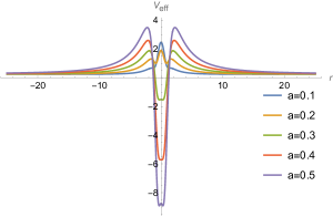
Figure 1: Effective potential $V_{eff}$ under the Kerr-like black bounce space-time scalar perturbation for different $a$ with $p=1,m=1,M=1,\mu=0.5,\Lambda_{lm}=2$.

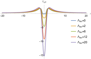
Figure 2: Effective potential $V_{eff}$ under the Kerr-like black bounce space-time scalar perturbation for different $\Lambda_{lm}$ with $a=0.3,p=1,m=1,M=1,\mu=0.5$.

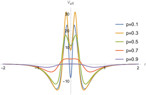
Figure 3: Effective potential $V_{eff}$ under the Kerr-like black bounce space-time scalar perturbation for different $p$ with $a=0.3,m=1,M=1,\mu=0.5,\Lambda_{lm}=2$.

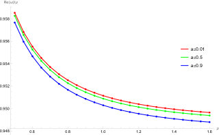
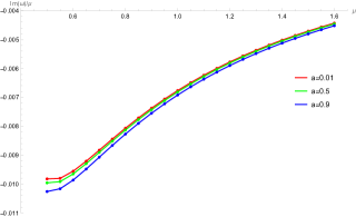
Figure 4: Frequency spectrum of scalar perturbation of rotating black bounce space-time for different $a$ with $m=1,M=1,p=1,\Lambda_{lm}=2$. The top panel is the oscillation frequency Re$\omega$/$\mu$, and bottom panel is the damping rate Im$\omega$/$\mu$, as the function of mass $\mu$.

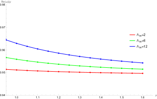
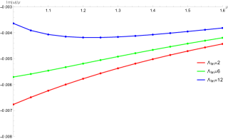
Figure 5: Frequency spectrum of scalar perturbation of rotating black bounce space-time for different $\Lambda_{lm}$ with $a=0.1,m=1,M=1,p=0.5$. The top panel is the oscillation frequency Re$\omega$/$\mu$, and bottom panel is the damping rate Im$\omega$/$\mu$, as the function of mass $\mu$.

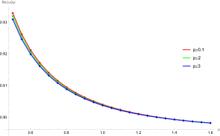
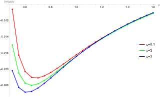
Figure 6: Frequency spectrum of scalar perturbation of rotating black bounce space-time for different $p$ with $a=0.1,m=1,M=1,\Lambda_{lm}=2$. The top panel is the oscillation frequency Re$\omega$/$\mu$, and bottom panel is the damping rate Im$\omega$/$\mu$, as the function of mass $\mu$.

IV QNM of the Kerr-like black bounce space-time

In this section, we briefly introduce Pöschl-Teller potential approximation and semi-analytic WKB method for calculating quasinormal modes of the Kerr-like black bounce space-time. We first introduce the relatively simple Pöschl-Teller potential approximation, which was suggested by B. Mashhoon Blome and Mashhoon (1984); Ferrari and Mashhoon (1984). This method is mainly realized by approximating the effective potential, i.e. Pöschl-Teller potential, and its usual form is

$$V_{PT}\left(r_{*}\right)=\frac{V_{0}}{\cosh^{2}\left(\frac{r_{*}}{b}\right)},$$ (20)

where

$$b=\frac{1}{\sqrt{-\frac{1}{2V_{0}}\frac{d^{2}V\left(r_{0*}\right)}{dr_{*}^{2}}}},$$ (21)

$r_{0*}$ represents the position of the maximum value $V\left(r_{*}\right)$. We use $V_{0}$ to denote the maximum value of the effective potential. The basic computational idea is that map Eq. (18) to a Schrödinger-like wave equation, so that the solution of equation (18) satisfying the boundary condition

$$R\left(r_{*}\right)\propto e^{i\omega r_{*}},\text{ for }r_{*}\rightarrow\infty,$$ (22)

$$R\left(r_{*}\right)\propto e^{-i\omega r_{*}},\text{ for }r_{*}\rightarrow-\infty.$$

Then, Eq. (18) can be mapped to the bound state of the new equation. One can analytically compute the bound states of the Schrödinger equation, so after obtaining them, we can obtain the QNM by considering the inverse mapping. To achieve this, the following transformations need to be considered

$$r_{*} \rightarrow-ir_{*},$$ (23)

$$\left(V_{0},b\right) \rightarrow\left(V_{0},-ib\right).$$

To remove the complexity of the expression, we let $p=\left(V_{0},b\right)$ and $p^{\prime}=\left(V_{0},-ib\right)$, therefore we have

$$V\left(-ir_{*},p^{\prime}\right)=V\left(r_{*},p\right).$$ (24)

Moreover, by the definition

$$\phi\left(r_{*},p\right)=\psi\left(-ir_{*},p^{\prime}\right),$$ (25)

$$\Omega(p)=\omega\left(p^{\prime}\right),$$

$\phi$ satisfies the equation

$$\frac{d^{2}\phi}{dr_{*}^{2}}+\left(-\Omega^{2}+V\right)\phi=0,$$ (26)

where

$$\Omega_{n}\left(V_{0},b\right)=\frac{1}{b}\left[-\sqrt{\frac{1}{4}+V_{0}b^{2}}+\left(n+\frac{1}{2}\right)\right].$$ (27)

Therefore, we can get the QNM

$$\omega_{n}\left(V_{0},b\right)=\Omega_{n}\left(V_{0},ib\right)=\frac{1}{b}\left[\pm\sqrt{V_{0}b^{2}-\frac{1}{4}}-\left(n+\frac{1}{2}\right)i\right]$$ (28)

with the $n$ being the integer $n\geq 0$.

On the other hand, in order to verify the accuracy of the results of the Pöschl-Teller potential approximation, we also use the WKB method Konoplya et al. (2019b); Konoplya and Zhidenko (2011). In the third order WKB method, we can obtain the QNM frequencies from the following equation

$$\omega^{2}=\left[V_{0}+\sqrt{-2V_{0}^{{}^{\prime\prime}}}\Lambda(n)-i\left(n+\frac{1}{2}\right)\sqrt{-2V_{0}^{{}^{\prime\prime}}}(1+\Omega(n))\right],$$ (29)

where

$$\Lambda(n)=\frac{1}{\sqrt{-2V_{0}}}\left[\frac{1}{8}\left(\frac{V_{0}^{(4)}}{V_{0}^{\prime}}\right)\left(\frac{1}{4}+\alpha^{2}\right)-\frac{1}{288}\left(\frac{V_{0}^{\prime}}{V_{0}^{\prime}}\right)^{2}\left(7+60\alpha^{2}\right)\right],$$ (30)

with

$$\Omega(n)=\frac{1}{-2V_{0}^{\prime}}\left[\frac{5}{6912}\left(\frac{V_{0}^{\prime}}{V_{0}^{\prime}}\right)^{4}\left(77+188\alpha^{2}\right)-\frac{1}{384}\left(\frac{V_{0}^{2}V_{0}^{(4)}}{V_{0}^{3}}\right)\left(51+100\alpha^{2}\right)+\right.$$ (31)

$$\left.\frac{1}{2304}\left(\frac{V_{0}^{(4)}}{V_{0}^{\prime}}\right)^{2}\left(67+68\alpha^{2}\right)+\frac{1}{288}\left(\frac{V_{0}^{\prime}V_{0}^{(5)}}{V_{0}^{2}}\right)\left(19+28\alpha^{2}\right)-\frac{1}{288}\left(\frac{V_{0}^{(6)}}{V_{0}^{\prime}}\right)\left(5+4\alpha^{2}\right)\right],$$

where prime represents the derivation respect to $r_{*}$, and $\alpha=n+\frac{1}{2}$. $V_{0}^{(n)}$ denotes the $n$-order derivative of the effective potential. Moreover, sixth order WKB method is given by

$$\frac{i(\omega^{2}-V_{0})}{\sqrt{-2V_{0}^{{}^{\prime\prime}}}}-\sum^{6}_{i=2}\Lambda_{i}=n+\frac{1}{2},\quad n=0,1,2,\cdots,$$ (32)

where the WKB corrections term $\Lambda_{i}$ is given in Ref. Iyer and Will (1987), and $V_{0}$ denotes the maximum of effective potential. In TABLE 1, we compare the QNM frequencies calculated by the above two methods, and one can find that the results of the Pöschl-Teller potential approximation are in good agreement with the results of the semi-analytic WKB method. Furthermore, the results show that with the increase of the spin parameter $a$, the actual oscillation frequencies and damping rate of the quasinormal modes in Kerr-like black bounce space-time will decrease, that is, they are inversely proportional to the spin parameter $a$. This demonstrates that when the Kerr-like black bounce space-time rotates faster, its decay rate is slower after perturbations. In Fig. 4, we show the actual oscillation frequencies and the damping rate of scalar perturbation of rotating black bounce space-time for different spin $a$ with $m=1,M=1,p=1,\Lambda_{lm}=2$. In Fig. 5, the frequency spectrum of scalar perturbation of rotating black bounce space-time for different $\Lambda_{lm}$ with $a=0.1,m=1,M=1,p=0.5$ are presented. In Fig. 6, we give the frequency spectrum of scalar perturbation of rotating black bounce space-time for different $p$ with $a=0.1,m=1,M=1,\Lambda_{lm}=2$.

Table 1: QNM frequencies of scalar field perturbation for $l=1,m=0,p=1,\mu=0$.

$a$	Pöschl-Teller	3th order WKB	6th order WKB
0.0	0.27997 - 0.096956i	0.271768 - 0.0937156i	0.274464 - 0.093496i
0.1	0.279558 - 0.0967096i	0.271429 - 0.0935124i	0.274117 - 0.0932881i
0.2	0.278329 - 0.0959766i	0.270418 - 0.0929065i	0.273079 - 0.0926693i
0.3	0.276305 - 0.0947754	0.268743 - 0.0919089i	0.271359 - 0.0916531i
0.4	0.273517 - 0.0931353i	0.266422 - 0.0905372i	0.268974 - 0.0902618i
0.5	0.270009 - 0.0910954i	0.263478 - 0.0888155i	0.265947 - 0.0885243i
0.6	0.265836 - 0.0887018i	0.25994 - 0.0867728i	0.262307 - 0.0864758i
0.7	0.261057 - 0.0860059i	0.255842 - 0.0844428i	0.258091 - 0.0841548i
0.8	0.255737 - 0.0830621i	0.251223 - 0.0818623i	0.253341 - 0.0816021i
0.9	0.249943 - 0.0799257i	0.246125 - 0.0790703i	0.248105 - 0.078859i

V Summary

In this work, we investigate the quasinormal modes of Kerr-like black bounce spacetime using the Pöschl-Teller potential approximation and semi-analytic WKB method to reach our main goal which is to check the parameters $\mu$ and $p$ that quantifies deviations from Kerr black hole. To do so, first we derive the effective potential for Kerr-like black bounce spacetime using scalar perturbation and plot the effective potential to visualize it. As far as the shape of the effective potential is concerned, it is completely different from the effective potential of some Kerr-like black hole spacetimes in modified gravity theories Sharif and Ama-Tul-Mughani (2020) and other rotating black holes in a dark matter halo Liu et al. (2022). In addition, we summarize the QNM frequencies calculated using the Pöschl-Teller potential approximation and WKB method in TABLE 1. At the same time, we plot the real and imaginary parts of the QNM frequencies in Fig.4-6. Our results demonstrate that for a fixed $\mu$, as spin $a$ increases, the true oscillation frequency decreases while the decay rate increases under the mass scalar field perturbations in Kerr-like black bounce spacetime. Increasing the parameter $p$, which determines whether spacetime is a black hole or a wormhole, makes the QNM frequency behave the same. In future studies, we expect to detect echoes in this rotating black bounce spacetime, as it exhibits a double-peaked effective potential like the Schwarzschild-like black bounce spacetime Churilova and Stuchlik (2020); Yang et al. (2021). Laser Interferometer Space Antenna (LISA), which is planned to be a space-based detector, could be detect low-frequency gravitational waves and may find some hints about the deviations from Kerr black hole and modified gravity theories Barausse et al. (2020).