Towards Lossless Conversion under Ultra-Low Latency for Spiking Neural Network with Dual-Phase Optimization

Abstract

Spiking neural network (SNN) operating with asynchronous discrete events shows higher energy efficiency. A popular approach to implementing deep SNNs is ANN-SNN conversion combining both efficient training of ANNs and efficient inference of SNNs. However, due to the intrinsic difference between ANNs and SNNs, the accuracy loss is usually non-negligible, especially under low simulating steps. It restricts the applications of SNN on latency-sensitive edge devices greatly. In this paper, we identify such performance degradation stems from the misrepresentation of the negative or overflow residual membrane potential in SNNs. Inspired by this, we systematically analyze the conversion error between SNNs and ANNs, and then decompose it into three folds: quantization error, clipping error, and residual membrane potential representation error. With such insights, we propose a dual-phase conversion algorithm to minimize those errors separately. Besides, we show each phase achieves significant performance gains in a complementary manner. We evaluate our method on challenging datasets including CIFAR-10, CIFAR-100, and ImageNet datasets. The experimental results show the proposed method achieves the state-of-the-art in terms of both accuracy and latency with promising energy preservation compared to ANNs. For instance, our method achieves the accuracy of $73.20\%$ on CIFAR-100 in only 2 time steps with $15.7\times$ less energy consumption.

Introduction

Spiking neural networks (SNNs), inspired by mimicking the dynamics of biological neurons (Hodgkin and Huxley 1952), have gained increasing interest (Roy, Jaiswal, and Panda 2019). Different from the computation with single, continuous-valued activation in ANNs, SNNs use binary spikes to transmit and process information. Each neuron in the SNNs will remain silent without energy consumption until receiving a spike/event afferent (Christensen et al. 2022). Such an event-driven computing paradigm enables more power-efficient solutions on dedicated neuromorphic hardware by substituting dense multiplication with sparse addition (Han, Srinivasan, and Roy 2020). As reported in (Davies et al. 2021; Merolla et al. 2014), SNNs on specified neuromorphic processors could achieve orders of magnitude lower energy consumption and latency compared with ANNs. In addition, SNNs could synergistically help denoise redundant information with inherent temporal dynamics (Deng et al. 2020). However, it still remains an open problem about how to obtain highly-performance SNNs efficiently.

In general, there are two mainstream methodologies for developing deep supervised SNNs up to date: (1) direct training for SNNs (2) converting ANNs into SNNs. For direct training methods, the back-propagation algorithm could not be applied to SNNs as spiking activation functions are inherently non-differentiable. Although some researchers have proposed some schemes to circumvent this difficulty, such as surrogate gradient (Wu et al. 2018) and probabilistic smoothness (Gardner, Sporea, and Grüning 2015), it is still hard to train large-scale SNNs due to the limited memory capacity, the short-time dependency, and vanishing spike rate in deep networks. Moreover, training SNNs on GPU always require multiple computing and storage overhead (Li et al. 2021) without specified optimization for storage and operation with binary events.

The other called converting methods obtain SNNs from pretrained ANNs. It yields the best performing SNNs on large-scale datasets like ImageNet (Deng et al. 2009) with cheap training costs. The core idea of conversion is to establish the consistent relationship between activations of analog neurons and some kind of aggregate representation of spiking neurons, such as spike count (Wu et al. 2021), spike rate (Diehl et al. 2015; Rueckauer et al. 2017), and postsynaptic potential (PSP) (Deng and Gu 2021). With such clear criteria, ANN-SNN conversion has been applied to complex scenarios with competitive performances compared to ANNs (Kim et al. 2020; Tan, Patel, and Kozma 2021; Luo et al. 2021; Kim, Venkatesha, and Panda 2022). Nevertheless, to achieve enough representation precision, considerable simulation steps are usually required for nearly lossless conversion, known as accuracy-delay tradeoff. It restricts the practical application of SNNs greatly. A large body of recent work (Yan, Zhou, and Wong 2021; Li et al. 2021; Bu et al. 2022b; Ho and Chang 2021) proposes to alleviate this problem by exploiting the quantization and clipping properties of aggregation representations. Even though, there is still an obvious performance gap between ANNs and SNNs under low inference latency ($\leq$ 16 time steps). And the underlying cause for such degradation is still unclear.

In this paper, we identify that the conversion error under low time steps arises mainly from the misrepresentation of residual membrane potential, which could characterize accurately information loss between input and output of spiking neurons with asynchronous spike firing. Furthermore, we show the error regarding residual potential representation is complementary to quantization and clipping errors. Inspired by this, we propose an ANN-SNN conversion algorithm with dual-phase optimization for threefold errors which achieves surprising performance with extremely low inference delay. The main contributions of this work could be demonstrated as follows:

• We analyze the operator consistency between ANNs and SNNs theoretically and identify the neglected residual potential representation problem. Then we divide conversion errors into three folds: quantization error, clipping error, and residual potential representation error.

• We propose a dual-phase optimization scheme for the threefold errors towards lossless conversion under ultra-low inference delay. In the first phase, quantization-clipping functions with trainable thresholds and quantization noise are applied to finetune ANNs. In the second phase, we minimize the residual potential representation error with layer-wise calibrations on weights and initial membrane potential.

• We verify the effectiveness and efficiency of the proposed dual-phase scheme on the CIFAR-10, CIFAR-100 and ImageNet datasets. Experimental results show significant improvements in accuracy-latency tradeoffs compared to state-of-the-art conversion methods. For example, we achieve $70.13\%$ top-1 accuracy ($19.16\%$ improvements) on ImageNet with VGG-16 architecture under only 16 time steps.

Related Work

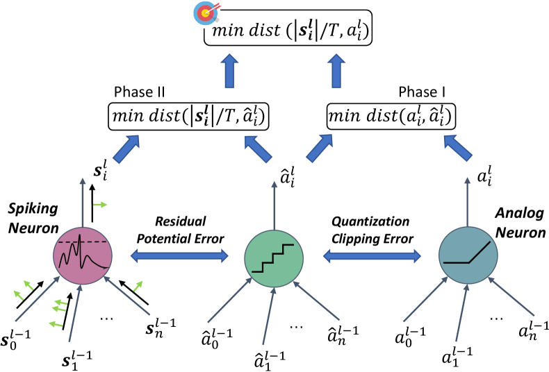
Figure 1: The criterion of conversion in this article is to minimize the distance of spike rates $r^{l}_{i}=|\boldsymbol{s}^{l}_{i}|/T$ and ANN activations $a^{l}_{i}$ by minimizing three errors with dual-phase methods at each layer. Here, $|\boldsymbol{s}^{l}_{i}|$ represents the cardinal number of spike train $\boldsymbol{s}^{l}_{i}$.

ANN-SNN Conversion.

Cao et al. (2015) first proposed to convert pretrained ANNs into SNNs and suggest the criterion of matching ANN activation and spiking rate of SNN. After the launch of ANN-SNN conversion, the development of conversion algorithms could be divided into two routes in general. From the perspective of constrained ANNs, Diehl et al. (2015) find the importance of weight-threshold balance and design weight normalization based on the maximum of layer-wise ANN activations. Afterward, a lot of works were dedicated to developing more elaborate normalization factors such as robust normalization (Rueckauer et al. 2017), spike-based normalization (Sengupta et al. 2019), channel-wise normalization (Kim et al. 2020), and normalization on shortcut connections (Hu, Tang, and Pan 2021). These methods can be sufficiently integrated with ReLU-based ANN to achieve lossless conversion. However, the inference delay is up to hundreds or thousands in general. Exploring the characteristics of quantization and clipping in spike rate, Yan, Zhou, and Wong (2021) proposed the training scheme with quantization and clipping constraints for ANNs, namely CQ-training. Similarly, Ding et al. (2021) proposed the method for weight and threshold training by stages to optimize the upper bound of the error between ReLU and CQ activations. Ho and Chang (2021) suggest a trainable clipping bound in activation functions to balance the threshold. Recently, Bu et al. (2022b) approximate the activation of SNNs through a quantization clip-floor-shift function and explores the conversion error when the quantization step in ANNs and time step in SNNs are mismatched. From the perspective of modified SNNs, The soft reset mechanism is widely adopted (Cao, Chen, and Khosla 2015; Han, Srinivasan, and Roy 2020) to avoid information loss from reset. Deng and Gu (2021) decomposed the network conversion error into the layer-wise conversion error and proposed the extra bias of $\theta/(2T)$ in spiking neurons to reduce the quantization error. Comparably, Hu (2021) and Bu (2022a) configured the initial membrane potential of spiking neurons as $\theta/2$ to reduce quantization error. Hwang et al. (2021) advised reducing inference latency by searching for the best initial membrane potential sequentially. Furthermore, Li et al. (2021) exploited the calibration effect of a handful of samples through activation transplanting to reduce clipping error and quantization error. Different from the previous methods, we put forward to minimize the neglected residual potential representation error simultaneously and make a step towards error-free ANN-SNN conversion under ultra-low latency.

Preliminaries

Analog Neuron Model.

Analog neurons in feedforward neural networks such as CNN, MLP et al communicate and learn with continuous activations. Mathematically, the forward computation of the $l$-th layer in feedforward networks could be formed as:

$$a_{i}^{l}=\sigma\left(z_{i}^{l}\right)=\sigma(\sum_{j}W_{ij}^{l}\cdot a_{j}^{l-1}+b_{i}^{l})$$ (1)

where $a^{l}_{i}$ is the output of ReLU activation function $\sigma(x)=\text{max}(0,x)$. $W^{l}_{ij}$ and $b^{l}_{i}$ are the weights and bias of neuron $i$ in the $l$-th layer respectively.

Spiking Neuron Model.

Integrate-and-Fire (IF) neuron model is widely used in conversion algorithms (Cao, Chen, and Khosla 2015; Rueckauer et al. 2017) because of the low computing cost and robust representation on firing rate. At each simulating time step $t$, the IF neuron $i$ receives afferent spikes $s^{l-1}_{i}[t]$ and updates its state $u^{l}_{i}[t]$ by integrating the input potential $v^{l}_{i}[t]$:

$$u_{i}^{l}[t]=\hat{u}_{i}^{l}[t-1]+v_{i}^{l}[t]=\hat{u}_{i}^{l}[t-1]+\sum_{j}W_{ij}^{l}s_{j}^{l-1}[t]+b_{i}^{l}$$ (2)

where $u^{l}_{i}[t]$ and $\hat{u}^{l}_{i}[t]$ denote the membrane potential before and after reset respectively. Then, the neuron will generate a spike $s_{i}^{l}[t]$ and reset the membrane potential whenever $u^{l}_{i}[t]$ exceeds the firing threshold $\theta^{l}_{i}$:

$$s_{i}^{l}[t]=\Theta\left(u_{i}^{l}[t]-\theta^{l}_{i}\right)\text{ with }\Theta(x)=\begin{cases}1,&\text{ if }x\geq 0\\ 0,&\text{ otherwise }\end{cases}$$ (3)

Specially, we adopt the widely used soft-reset (reset-by-subtraction) mechanism (Han, Srinivasan, and Roy 2020; Cao, Chen, and Khosla 2015). Formally, the soft reset mechanism could be presented as:

$$\hat{u}_{i}^{l}[t]=u_{i}^{l}[t]-s_{i}^{l}[t]\cdot\theta^{l}_{i}$$ (4)

Input and Readout.

Instead of explicit spike coding, we directly inject the image as input potential repeatedly into SNNs at each time step to avoid information loss. Meanwhile, the average input potential $\overline{v}^{l}_{i}=(\sum_{t=1}^{T}v^{l}_{i}[t])/T$ rather than spike rate $r^{l}_{i}=(\sum_{t}s^{l}_{i}[t])/T$ is read out in the last layer. More discussion can be found in Appendix-A.

Error Analysis

In this paper, our target is to build a consistent mapping between spike rates $r^{l}_{i}$ in SNNs and activation values $a^{l}_{i}$ in ANNs shown in Fig 1. Firstly, we derive the exact relation between average input potential $\overline{v}^{l}_{i}$ and input spike rate $r^{l-1}_{j}$:

$$\overline{v}_{i}^{l}=\frac{\sum_{t=1}^{T}\sum_{j}W_{ij}^{l}s_{j}^{l-1}[t]+b_{i}^{l}T}{T}=\sum_{j}W_{ij}^{l}r_{j}^{l-1}+b_{i}^{l}$$ (5)

Compared to Eq. 1, the functional relation between $\overline{v}^{l}_{i}$ and $r^{l-1}_{j}$ in IF neurons is identical to that between $z^{l}_{i}$ and $a^{l-1}_{j}$ in analog neurons. Then, the remained question is what is the difference between the function $\overline{v}^{l}_{i}\to r^{l}_{i}$ and the function $z^{l}_{i}\to a^{l}_{i}$? By substituting Eq. 4 to Eq. 2 and accumulating from $0$ to $T$, the relation (detailed derivation provided in Appendix-C) between $r^{l}_{i}$ and $r^{l-1}_{j}$ could be deduced as:

$$r_{i}^{l}=\sum_{j}\left(W_{ij}^{l}r_{j}^{l-1}+b_{i}^{l}\right)/\theta^{l}_{i}-\epsilon_{i}^{l}$$ (6)

where $\epsilon^{l}_{i}=\frac{\hat{u}^{l}_{i}[T]-\hat{u}^{l}_{i}[0]}{T\theta^{l}_{i}}$ is the component about residual membrane potential $\hat{u}^{l}_{i}[T]$. By substituting Eq. 5 into Eq. 6, we obtain the exact expression between $\overline{v}^{l}_{i}$ and $r^{l}_{i}$:

$$r_{i}^{l}=f_{\theta,T}\left(\overline{v}_{i}^{l},\epsilon_{i}^{l}\right)=\overline{v}_{i}^{l}/\theta^{l}_{i}-\epsilon_{i}^{l}$$ (7)

Remarkably, $\epsilon^{l}_{i}$ is highly nonlinear, nondifferentiable, and nonconvex as $\hat{u}^{l}_{i}[T]$ is calculated with the compound of $T$ Heaviside functions $\Theta(x)$. Therefore, the only divergence in operators appears between the equivalent activation function $f_{\theta,T}(x,\epsilon)$ in SNNs and $\sigma(x)$ in ANNs. To bypass the non-determinism and complexity of $\epsilon$, we start from the limited residual membrane potential assumption:

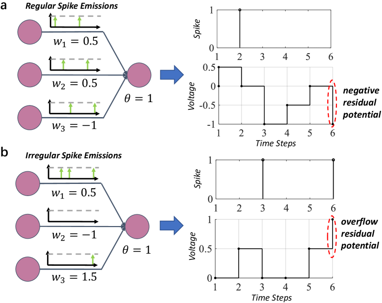
Figure 2: Two handcrafted examples to explain the residual membrane potential representation error.

$$0\leq\hat{u}_{i}^{l}[T]-\hat{u}_{i}^{l}[0]<\theta^{l}_{i}$$ (8)

Under such assumption, $\epsilon^{l}_{i}$ will be bounded in $[0,\frac{1}{T})$ while $r^{l}_{i}\in\{\frac{0}{T},\frac{1}{T},...,\frac{T}{T}\}$. So the nonlinearity of $f_{\theta,T}(x,\epsilon)$ could be downgraded to the floor function with quantization step $\theta/T$:

$$g_{\theta,T}(x)=\frac{1}{T}\left\lfloor x\frac{T}{\theta}\right\rfloor=\frac{1}{\theta}\lfloor x\rfloor_{\theta/T}$$ (9)

Furthermore, the spike rate clipping technique is adopted to compensate for the error between $f_{\theta,T}(x)$ and $g_{\theta,T}(x)$ when the condition of Eq. 8 is not satisfied.

$$g_{\theta,T}(x)=\operatorname{clip}\left(\frac{1}{\theta}\lfloor x\rfloor_{\theta/T},0,1\right)$$ (10)

However, the errors still exist and remain non-negligible even with such compensation. It is often considered as transient dynamics (Rueckauer et al. 2017), temporal jitter of spike trains (Wu et al. 2021) or unevenness error (Bu et al. 2022b) without dedicated optimization. However, we contend that it is more precise and tractable to attribute such error to incomplete representation of residual membrane potential rather than irregular discharge of spikes in IF models. To explain that, we handcraft two examples under uniform and irregular spikes distribution respectively in Fig. 2.

Example 1 (Regular Spike Emissions).

All the input neurons emit spikes regularly with an interval of 2 time steps in Fig.2a. However, the output of floor-clipping function $g_{\theta,T}(\overline{v})$ is 0 while the real spike rate $r=f_{\theta,T}(\overline{v},\epsilon)$ is $\frac{1}{6}.$ The spike rate is undervalued with negative residual potential even under such uniform spike afferents.

Example 2 (Irregular Spike Emissions).

The output neuron is under saturation state with real spike rate $r=\frac{2}{6}$ while the expectation $g_{\theta,T}(v)$ is $\frac{3}{6}$ in the example of Fig.2b. The spike rate is overvalued with overflow residual potential.

Therefore, the estimated spike rate may surpass or be below the real of IF neurons in both cases. The fundamental cause of the error comes from the IF neuron with soft-reset mechanism could not respond for the residual membrane potential out of $[0,\theta)$. Then we call the kind of error as residual membrane potential representation error, RPE in short. It evaluates the divergence between the real spike rate $f_{\theta,T}(x,\epsilon)$ and the estimated spike rate $g_{\theta,T}(x)$ as shown in Fig. 1. Besides, the quantization and flooring function $g_{\theta,T}(x)$ is divergent from the ReLU function $\sigma(x)$ commonly used by ANNs in operators. Li (2021) summarized similar errors in the PSP-based conversion algorithm as clipping error and flooring error. Here we denote them as clipping error, CE and quantization error, QE generally shown in Fig. 3.

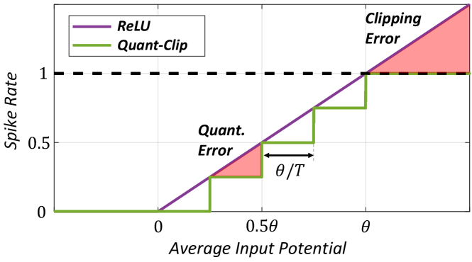
Figure 3: A schematic diagram illustrating quantization and clipping errors with spike rate representation.

Method

Based on the above error analysis, we propose a dual-stage conversion scheme (Fig. 4) towards lossless conversion by minimizing QE, CE, and RPE by stages. Overall, we starts from a source neural network using clipping function $\sigma(x)$ as the activation function, then transfer it to a neural network with trainable quantization-clipping activation function $g_{\theta,T}(x)$, called QC-ANN later. Therefore, the QE and CE could be optimized with the fine-tuning of the QC-ANN. Finally, the layer-wise calibration on weights and initial membrane potential is adopted to optimize the RPE based on the activation divergence between $g_{\theta,T}(x)$ and $f_{\theta,T}(\overline{v}^{l}_{i},\epsilon^{l}_{i})$.

Phase-I: QC-Fintuning with Trainable Threshold

The principle of the first phase is to minimize the QE and CE (right part of Fig. 1) and to take the quantization and clipping property of estimated activation function $g_{\theta,T}(x)$ for SNNs into ANN training. So we introduce the QC-ANN with trainable thresholds $\theta^{l}_{i}$ as the intermediate network.

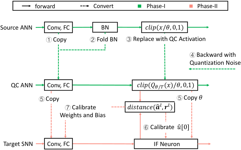
Figure 4: Overall flow combining dual-phase design.

Convert ANNs into QC-ANNs.

To avoid the high computational cost due to training from scratch with QC activation function $g_{\theta,T}(x)$ under different $T$, we start with training source ANNs with activation $\sigma(x)=\text{clip}(\frac{1}{\theta}x,0,1)$ unrelated to the specified time steps $T$. Then we convert the source ANN into QC-ANN by simply copying the network parameters and replacing the corresponding activation functions. Here, we adopt similarly shift term $\Delta x=\theta/(2T)$ proposed in (Deng and Gu 2021) to minimize the distance $||\sigma(x)-g_{\theta,T}(x+\Delta x)||^{2}$ under different time steps $T$. So the floor term in $g_{\theta,T}(x)$ is replaced by a round term:

$$g_{\theta,T}(x) =\operatorname{clip}\left(\frac{1}{\theta}Q_{\theta/T}(x),0,1\right)\text{ where }$$ (11)

$$Q_{\Delta}(x) =\Delta Q_{1}\left(\frac{x}{\Delta}\right)=\Delta\operatorname{round}\left(\frac{x}{\Delta}\right)$$

Fine-tuning with Quantization Noise.

Although the optimal shift is applied, the QE and CE still exist and contribute to the conversion error. So we finetune the QC-ANN after copying weights from source ANN and replacing the activation function $\sigma(x)$ with $g_{\theta,T}(x)$. However, the round term $Q(x)$ in $g_{\theta,T}(x)$ has null gradients which means the derivative of the input is zero almost everywhere. To train QC-ANN with such an ill-defined function, we adopt the widely used Straight Through Estimator (STE) (Bengio, Léonard, and Courville 2013) to estimate the gradients:

$$\frac{\partial Q_{\Delta}(x)}{\partial x}=\frac{\partial Q_{1}(x)}{\partial x}=\frac{\partial\lfloor x\rfloor}{\partial x}=1$$ (12)

Nevertheless, in the STE scheme, most weights are updated with biased gradients. It brings the larger bias with the increasing quantization step $\theta/T$ when time step is relatively low ($T<8$). Furthermore, the convergence of QC-ANN and the fast-inference ability of target SNNs are limited inevitably. So we propose to correct the biased gradient using the noisy quantization function $\hat{Q}(x)$ inspired by (Fan et al. 2020) which introduces Quant-Noise in model compression. Specifically, we replace a random fraction of $Q(x)$ with the identity mapping $x$ at each forward:

$$\hat{Q}(x)=x+(Q(x)-x)\cdot M,\quad M\sim\operatorname{Bernoulli}(p)$$ (13)

Thus, most weights in QC-ANN are updated with unbiased gradients boosting the convergence under large quantization step.

Phase-II: Layer-wise Calibration with BPTT

After copying the weights, biases and thresholds trained in QC-ANN into target SNN, we get an SNN without considering RPE. To optimize RPE, the core objective of the second stage shown in the left part of Fig. 1, we adopt a layer-wise calibration mechanism on weights $\boldsymbol{W}$ and initial membrane potential $\hat{\boldsymbol{u}}[0]$. Firstly, we modify the real activation function $f_{\theta,T}(x)$ on spike rate according to the shift $\theta/(2T)$ presented in $g_{\theta,T}(x)$:

$$f_{\theta,T}(\overline{v},\epsilon)=\left(\overline{v}+\frac{\theta}{2T}\right)/\theta-\epsilon$$ (14)

Coarse Calibration (CC) on Initial Membrane Potential.

When the condition Eq. 8 is not satisfied, the initial membrane potential $\hat{\boldsymbol{u}}^{l}[0]$ at the $l$-th layer could play a coarse adjustment role for the activation distribution (Eq. 6). Considering the calibration on $N$ samples, the core for calibrating $\hat{\boldsymbol{u}}[0]$ lies in solving the following optimization equation:

$$\min_{\hat{\boldsymbol{u}}[0]}\left\{\sum_{i=1}^{N}\left(\frac{\overline{\boldsymbol{v}}_{i}}{\theta}+\frac{1}{2T}-\frac{\hat{\boldsymbol{u}}_{i}[T]-\hat{\boldsymbol{u}}[0]}{T\theta}-g_{\theta,T}\left(\boldsymbol{z}_{i}\right)\right)^{2}\right\}$$ (15)

Suppose $\hat{\boldsymbol{u}}[T]$ is unrelated to $\hat{\boldsymbol{u}}[0]$, then the problem turns into a linear form and the corresponding solution is:

$$\hat{\boldsymbol{u}}[0] =\frac{T\theta}{N}\sum_{i=1}^{N}\left(g_{\theta,T}\left(\boldsymbol{z}_{i}\right)-f_{\theta,T}\left(\overline{\boldsymbol{v}}_{i},\epsilon_{i}|\hat{\boldsymbol{u}}[0]=\boldsymbol{0}\right)\right)$$ (16)

$$=\frac{T\theta}{N}\sum_{i=1}^{N}\left(\hat{\boldsymbol{a}}_{i}-\boldsymbol{r}_{i}\right)$$

By the way, we could correct roughly the output expectation of the target SNN as that of the QC-ANN.

Fine Calibration (FC) on Weights and Bias.

To calibrate the RPE more precisely, we measured the KL divergence between target activation $\boldsymbol{\hat{a}^{l}}$ and real spike rate $\boldsymbol{r^{l}}$ here:

$$\min_{\boldsymbol{W}}\mathcal{L}\left(\boldsymbol{r}^{l},\hat{\boldsymbol{a}}^{l}\right)=D_{\text{KL}}\left(\hat{\boldsymbol{a}}^{l}\|\boldsymbol{f}_{\theta,T}\left(\overline{\boldsymbol{v}}^{l}(\boldsymbol{W}),\boldsymbol{\epsilon}^{l}(\boldsymbol{W})\right)\right)$$ (17)

Although $\overline{\boldsymbol{v}}^{l}$ is the linear combination of $\boldsymbol{W}^{l}$, $\boldsymbol{\epsilon}^{l}$ is a superposition of nondifferentiable Heaviside functions $\Theta(x)$. In order to solve such nonconvex and nondifferentiable optimization problems, we adopt a rectangular surrogate gradient $h(u)$ (Wu et al. 2019) to replace the illness gradient $\frac{\partial\Theta(u)}{\partial u}$:

$$\frac{\partial\Theta(u)}{\partial u}\approx h(u)=\frac{1}{\alpha}\operatorname{sign}\left(|u-\theta|<\frac{\alpha}{2}\right)$$ (18)

where $\alpha$ controls the smoothness degree for $\frac{\partial\Theta(u)}{\partial u}$. Then we could obtain the gradients of weights with backpropagation-through-time (BPTT):

$$\frac{\partial\mathcal{L}}{\partial W_{ij}^{l}} =\frac{1}{T}\frac{\partial\mathcal{L}}{\partial r_{i}^{l}}\sum_{t^{*}=1}^{T}\sum_{t=1}^{t^{*}}\frac{\partial s_{i}^{l}\left[t^{*}\right]}{\partial u_{i}^{l}[t]}s_{j}^{l-1}[t]$$ (19)

$$\frac{\partial s_{i}^{l}\left[t^{*}\right]}{\partial u_{i}^{l}[t]} =\begin{cases}h\left(u_{i}^{l}\left[t^{*}\right]\right)&\text{ if }t=t^{*}\\ \frac{\partial s_{i}^{l}\left[t^{*}\right]}{\partial u_{i}^{l}[t+1]}\left(1-\theta_{i}^{l}h\left(u_{i}^{l}[t]\right)\right)&\text{ if }t<t^{*}\end{cases}$$

Compared to the direct training with surrogate gradients using BPTT, our calibration methods here only feedforward and backward on one layer which means the spatial complexity is $O(T\cdot\text{max}_{l}(n_{l}))$ rather than $O(T\cdot\sum_{l}n_{l})$ where $n_{i}$ is the neurons number at the $l$-th layer in ANNs. Moreover, it is much easier and more computationally efficient to converge by fine-tuning on a pretrained layer rather than retraining from scratch on a large network presented in surrogate gradient methods. Empirically, it is enough for the calibration with several hundred of samples.

Experiments

Method	Architecture	ANN Acc.	$T=2$	$T=4$	$T=8$	$T=16$	$T=32$	$T=64$	$T\geq 128$
RMP (Han, Srinivasan, and Roy 2020)†	ResNet-20	91.47	-	-	-	-	-	-	91.36
TSC (Han and Roy 2020)†	ResNet-20	91.47	-	-	-	-	-	69.38	91.42
OPT (Deng and Gu 2021)	ResNet-20	95.46	-	-	-	-	84.06	92.48	95.30
CAP (Li et al. 2021)	ResNet-20	95.46	-	-	-	-	94.78	95.30	95.45
RNL (Ding et al. 2021)	PreActResNet-18	93.06	-	-	-	47.63	83.95	91.96	93.41
OPI (Bu et al. 2022a)	ResNet-18	96.04	-	-	75.44	90.43	94.82	95.92	96.08
QCFS (Bu et al. 2022b)	ResNet-18	96.04	75.44	90.43	94.82	95.92	96.08	96.06	96.06
Ours	ResNet-18	96.41	89.97	93.27	95.36	96.28	96.44	96.49	96.43
	ResNet-20	96.66	90.43	93.27	95.46	96.30	96.60	96.71	96.76
TSC (Han and Roy 2020)	VGG-16	93.63	-	-	-	-	-	92.79	93.63
RMP (Han, Srinivasan, and Roy 2020)		93.63	-	-	-	-	60.30	90.35	93.63
OPT (Deng and Gu 2021)		95.72	-	-	-	-	76.24	90.64	95.73
CAP (Li et al. 2021)		95.72	-	-	-	-	93.71	95.14	95.79
RNL (Ding et al. 2021)		92.82	-	-	-	57.90	85.40	91.15	92.51
OPI (Bu et al. 2022a)		94.57	-	-	90.96	93.38	94.20	94.45	94.55
QCFS (Bu et al. 2022b)		95.52	91.18	93.96	94.95	95.40	95.54	95.55	95.59
Ours	VGG-16	95.73	91.71	94.06	95.26	95.55	95.71	95.78	95.81

Table 1: Tradeoff between accuracy and inference delay on CIFAR-10 dataset. $\dagger$ means using standard ResNet-20 architecture while others construct ResNet-20 by adding two more layers to the ResNet-18.

In this section, we evaluate the effectiveness and efficiency of the proposed dual-phase method compared to other state-of-art conversion algorithms on CIFAR-10, CIFAR-100 and ImageNet datasets. Meanwhile, we use the widely adopted VGG and ResNet architectures in the existing literature.

Implementation Details

Training of Source ANN.

To obtain a high-performance source ANN trained with $\sigma(x)=\text{clip}(\frac{1}{\theta}x,0,1)$. In general, there are three approaches: (1) Training an ANN with clipping function $\sigma(x)$ directly as done in (Deng and Gu 2021). (2) training an ANN with ReLU function and then constrain the activations into $[0,1]$ with weight-threshold balancing technique (Diehl et al. 2015; Rueckauer et al. 2017). (3) Training an ANN with the rescaled clipping function $\sigma(x)=\text{clip}(x,0,\theta)$ (Ho and Chang 2021) and then fusing the scale factor $\theta$ into weights after training. A detailed comparison of three methods considering threefold errors is provided in Appendix-D. In experiments, we adopt the first method for CIFAR-10. For CIFAR-100 and ImageNet, we use the third method to achieve higher performance.

Experiments Settings.

For CIFAR-10 and CIFAR-100, we crop images into 32$\times$32 with the padding of 4 pixels and flip them horizontally at random. Besides, as done in (Li et al. 2021; Bu et al. 2022b), we adopt the data augmentation of Cutout (DeVries and Taylor 2017) and AutoAugment (Cubuk et al. 2019) to increase the generalization ability of source ANNs. For ImageNet, we adopt the standard pre-processing pipeline and crop images into 224$\times$224.

For training source ANN, we initialize the learning rate as 0.1 and then update it through the SGD optimizer with the momentum of 0.9. Meanwhile, the weight decay is set to $5e-4$ to regularize the network. Besides, the learning rate is set as $1e-4$ further to finetune QC-ANN. For CIFAR-10, the probability of quantization noise $p$ is set as 0.1 and 0.2 when $T\leq 4$. Otherwise, no noise will be injected into QC-ANNs. The $p$ is set as 0.1 across all time steps on ImageNet and CIFAR-100 datasets. For Phase-II, we adopt Adam as the optimizer with an initial learning rate of 5e-4. The weight decay is set as 0. Moreover, we also adopt layer-wise BPTT calibration on the initial potential for ImageNet.

Alation Study

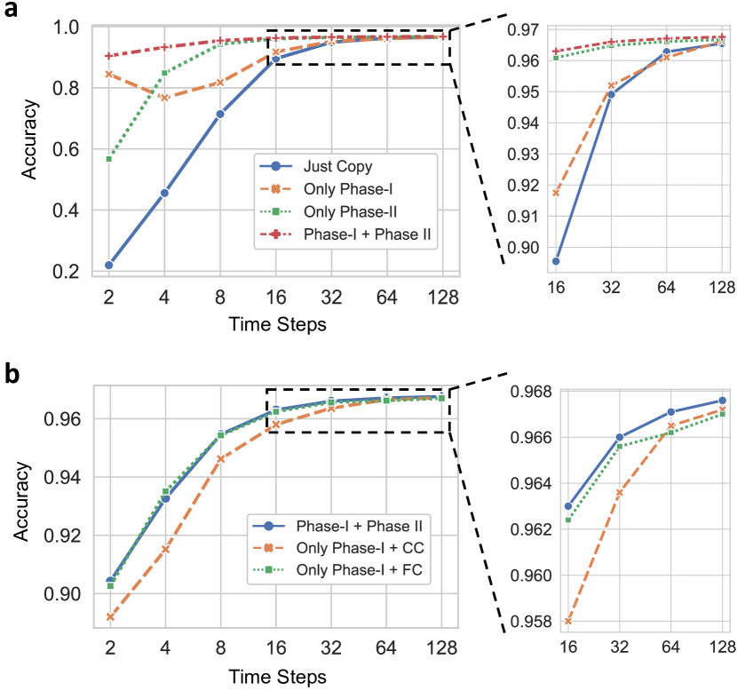
Figure 5: Exploring the effect of each component.

In this section, we conduct a series of ablation studies and show the proposed method reduces the conversion loss in a complementary manner. Specially, we test ResNet-20 on CIFAR-10 from $T=2$ to $T=128$ under six conditions: Just Copy Weights, Only Phase I, Only Phase II, Phase I + Phase II, Phase-I + CC, and Phase-I + FC. Detailed statistics are provided in Appendix-E.

As shown in Fig. 5a, both Only Phase I and Only Phase II improve the performance effectively, which is especially impressive when $T\leq 32$. Besides, Phase-I + Phase-II with dedicated optimization obtains the best results across all time steps which indicates the synergic effect of the two phases. Comparing the two phases individually, we find Phase-I optimizing the QE and CE could achieve better results when $T<4$. Otherwise, Phase-II optimizing RPE mainly could obtain higher performance. It is interpretable as the decrease of $T$ will increase the quantization factor $\theta/T$ and the QE naturally. So the performance degradation stemmed from the QE plays a dominant role compared to RPE when $T$ is extremely low. Surprisingly, Only Phase-II could achieve the similar performance of Phase I + Phase II with just 8 time steps while Only Phase-I needs 32 time steps. It demonstrates that optimizing RPE is more efficient in low-latency conversion in general. So simply adopting layer-wise Phase-II with a handful of samples is enough for conversion on resource-constrained devices. Notably, there is a strange accuracy drop for Only Phase-I when $T=4$. It may come from increasing RPE which is not optimized by Phase-I. Therefore, the error could be compensated by Phase-II shown in the curve of Phase-I + Phase-II.

To understand the effect of each component in Phase-II further, we do coarse calibration and fine calibration separately after Phase-I (Fig. 5b). In general, both components improve performance consistently. Specially, we find Phase I + FC can achieve extremely close results to Phase I + Phase II. And it even outperforms Phase-I + Phase-II when $T=4$. Nevertheless, coarse calibration still provides a lightweight solution without gradient computation and a proper initialization for fine calibration.

Tradeoff between Accuracy and Inference Delay

Method	Architecture	ANN Acc.	$T=4$	$T=8$	$T=16$	$T=32$	$T=64$	$T=128$	$T\geq 256$
RMP (Han, Srinivasan, and Roy 2020)	ResNet-34	70.64	-	-	-	-	-	-	69.89
TSC (Han and Roy 2020)		70.64	-	-	-	-	-	-	69.93
TCL (Ho and Chang 2021)		70.85	-	-	-	-	-	-	70.66
OPT (Deng and Gu 2021)		75.66	-	-	-	0.09	0.12	3.19	75.08
CAP (Li et al. 2021)		75.66	-	-	-	64.54	71.12	73.45	75.45
QCFS (Bu et al. 2022b)		74.32	-	-	59.35	69.37	72.35	73.15	73.39
Ours	ResNet-34	73.43	55.71	61.20	67.77	71.66	72.65	73.37	73.45
RMP (Han, Srinivasan, and Roy 2020)	VGG-16	73.49	-	-	-	-	-	-	73.09
TSC (Han and Roy 2020)		73.49	-	-	-	-	-	-	73.46
OPT (Deng and Gu 2021)		75.36	-	-	-	0.114	0.118	0.122	73.88
CAP (Li et al. 2021)		75.36	-	-	-	63.64	70.69	73.32	75.32
QCFS (Bu et al. 2022b)		74.29	-	-	50.97	68.47	72.85	73.97	74.32
OPI (Bu et al. 2022a)		74.85	-	6.25	36.02	64.70	72.47	74.24	74.69
Ours	VGG-16	74.88	59.95	62.51	70.13	73.44	74.68	74.93	74.94

Table 2: Tradeoff between accuracy and inference delay on ImageNet Dataset.

We compare the proposed method with the state-of-the-art methods on CIFAR-10 (Table 1) and ImageNet (Table 2). More results on CIFAR-100 are provided in Appendix-F.

In general, our method achieves the best result nearly across all time steps. For ultra-low latency $T=2$ and $T=4$, our method achieves promising performance improvements of $14.53\%$ and $2.84\%$ with ResNet-18 on CIFAR-10 dataset respectively. The superiority seems to vanish when $T\geq 8$ compared to the most recent work (Bu et al. 2022b). However, when considering large-scale datasets like ImageNet, the proposed method can still improve the state-of-the-art of accuracy-delay tradeoff sustainedly (Table. 2). For instance, the inference delay is shrunk by $4\times$ into 4 time steps on ImageNet with VGG16 architecture while still obtaining the significant performance improvements (8.98% top-1 at least) compared to the existing literature. Notably, as we do not apply the CollorJitter data augmentation as done in (Li et al. 2021; Bu et al. 2022a), the result of source ANN on ImageNet is slightly lower than the best results reported. Even though, our method still outperforms previous works and achieves 73.44% top-1 accuracy under relatively long time steps ($T=32$). Besides, our method is still competitive compared to the state-of-the-art direct training method characterized by temporal credit assignment under only $4$ time steps on both CIFAR datasets. All those results illustrate the effectiveness of optimizing threefold errors simultaneously.

Effect of Different Sample Numbers

# of samples	ResNet-18 (96.41)				VGG-16 (95.73)
	$T=2$	$T=4$	$T=8$		$T=2$	$T=4$	$T=8$
0	76.01	66.52	84.17		88.89	92.89	92.72
16	87.89	90.47	94.31		88.96	91.79	94.31
32	88.75	91.94	94.89		90.21	93.24	94.41
64	89.56	92.40	94.85		90.59	93.19	94.80
128	89.74	92.18	95.07		90.91	93.54	95.01
256	89.51	92.77	95.29		90.80	94.04	95.02
512	89.89	92.96	95.31		91.41	94.13	95.22
1024	90.49	93.23	95.35		90.98	93.60	95.04

Table 3: The effect of calibration number $N$. The number in parentheses imply the accuracy of source ANN.

As shown in Table 3, we explore the effect of calibration numbers on CIFAR-10 with both ResNet-34 and VGG-16. Surprisingly, a few calibration samples could bring significant improvements. For example, the performance of spiking ResNet-18 under 4 time steps is improved by 25.42% with only 32 samples. It shows the efficiency of the proposed BPTT calibration, especially for low-latency conversion.

Energy-Efficiency and Sparsity

	ANN	$T=2$	$T=4$	$T=8$
GSOP ($\times$ 1e-3)	480.2	156.1 $\pm$ 6.3	238.9 $\pm$ 10.0	433.7 $\pm$ 17.2
Energy ($\mu\mathrm{J}$)	2208.7	140.5 $\pm$ 5.7	215.0 $\pm$ 9.0	356.0 $\pm$ 21.7
Energy Ratio (%)	100	6.36 $\pm$ 0.26	9.73 $\pm$ 0.41	16.11 $\pm$ 0.98
Accuracy (%)	79.22	73.20 (6.02)	75.98 (3.24)	78.84 (0.38)

Table 4: The energy cost compared to ANN counterparts under different time steps on CIFAR-100. The numbers in parentheses represent accuracy losses during conversion.

In this section, we count the total synaptic operations (SOP) to estimate the computation overhead of SNN compared to their ANN counterparts (Merolla et al. 2014) (More details could be found in Appendix-G). Especially, synaptic operation by accumulation (AC) in SNNs is variable with spike sparsity while synaptic operation by multiply and accumulation (MAC) in ANNs is constant given a particular network structure. Here, we measure 32-bit float-point AC and MAC by $\alpha_{\text{AC}}=0.9\ pJ$ and $\alpha_{\text{MAC}}=4.6\ pJ$ per operation individually (Han et al. 2015).

From Table 4, SNN is more SOP-efficient with sparse spike communications than the ANN in the same ResNet-18 architecture when $T\leq 8$. The energy efficiency is more significant considering the operation degrading from MAC to AC. For instance, the conversion is nearly lossless (0.38% accuracy loss) when $T=8$ with only $16\%$ energy consumption compared to the ANN counterpart. For edge devices with stringent power requirements, the energy consumption could be downgraded to 140 $\mu J$ further ( $15.7\times$ energy saving with 73%+ performance on CIFAR-100).

Conclusion

In this paper, instead of merely optimizing quantization and clipping error in the previous works, we identify the neglected residual membrane potential representation and take it into the design of conversion algorithms. As a result, we present a novel dual-phase converting algorithm to optimize threefold errors. Specifically, we introduce an intermediate neural network called QC-ANN to separate errors explicitly as well as the BPTT calibration to handle temporal dynamics in SNNs. Experimental results demonstrate our method improves accuracy-latency tradeoff greatly with attractive power conservation compared to ANNs. We believe this work shall help pave the way towards lossless ANN-SNN conversion under ultra-low latency.

References

- Bengio, Léonard, and Courville (2013) Bengio, Y.; Léonard, N.; and Courville, A. 2013. Estimating or propagating gradients through stochastic neurons for conditional computation. arXiv preprint arXiv:1308.3432.
- Bu et al. (2022a) Bu, T.; Ding, J.; Yu, Z.; and Huang, T. 2022a. Optimized Potential Initialization for Low-latency Spiking Neural Networks. In Proceedings of the AAAI conference on artificial intelligence.
- Bu et al. (2022b) Bu, T.; Fang, W.; Ding, J.; Dai, P.; Yu, Z.; and Huang, T. 2022b. Optimal ANN-SNN Conversion for High-accuracy and Ultra-low-latency Spiking Neural Networks. In International Conference on Learning Representations.
- Cao, Chen, and Khosla (2015) Cao, Y.; Chen, Y.; and Khosla, D. 2015. Spiking deep convolutional neural networks for energy-efficient object recognition. International Journal of Computer Vision, 113(1): 54–66.
- Christensen et al. (2022) Christensen, D. V.; Dittmann, R.; Linares-Barranco, B.; Sebastian, A.; Le Gallo, M.; Redaelli, A.; Slesazeck, S.; Mikolajick, T.; Spiga, S.; Menzel, S.; et al. 2022. 2022 roadmap on neuromorphic computing and engineering. Neuromorphic Computing and Engineering, 2(2): 022501.
- Cubuk et al. (2019) Cubuk, E. D.; Zoph, B.; Mane, D.; Vasudevan, V.; and Le, Q. V. 2019. Autoaugment: Learning augmentation strategies from data. In Proceedings of the IEEE/CVF Conference on Computer Vision and Pattern Recognition, 113–123.
- Davies et al. (2021) Davies, M.; Wild, A.; Orchard, G.; Sandamirskaya, Y.; Guerra, G. A. F.; Joshi, P.; Plank, P.; and Risbud, S. R. 2021. Advancing neuromorphic computing with loihi: A survey of results and outlook. Proceedings of the IEEE, 109(5): 911–934.
- Deng et al. (2009) Deng, J.; Dong, W.; Socher, R.; Li, L.-J.; Li, K.; and Fei-Fei, L. 2009. Imagenet: A large-scale hierarchical image database. In 2009 IEEE conference on computer vision and pattern recognition, 248–255. Ieee.
- Deng et al. (2020) Deng, L.; Wu, Y.; Hu, X.; Liang, L.; Ding, Y.; Li, G.; Zhao, G.; Li, P.; and Xie, Y. 2020. Rethinking the performance comparison between SNNS and ANNS. Neural networks, 121: 294–307.
- Deng and Gu (2021) Deng, S.; and Gu, S. 2021. Optimal Conversion of Conventional Artificial Neural Networks to Spiking Neural Networks. In International Conference on Learning Representations.
- DeVries and Taylor (2017) DeVries, T.; and Taylor, G. W. 2017. Improved regularization of convolutional neural networks with cutout. arXiv preprint arXiv:1708.04552.
- Diehl et al. (2015) Diehl, P. U.; Neil, D.; Binas, J.; Cook, M.; Liu, S.-C.; and Pfeiffer, M. 2015. Fast-classifying, high-accuracy spiking deep networks through weight and threshold balancing. In 2015 International joint conference on neural networks (IJCNN), 1–8. ieee.
- Ding et al. (2021) Ding, J.; Yu, Z.; Tian, Y.; and Huang, T. 2021. Optimal ann-snn conversion for fast and accurate inference in deep spiking neural networks. In IJCAI.
- Fan et al. (2020) Fan, A.; Stock, P.; Graham, B.; Grave, E.; Gribonval, R.; Jegou, H.; and Joulin, A. 2020. Training with quantization noise for extreme model compression. arXiv preprint arXiv:2004.07320.
- Gardner, Sporea, and Grüning (2015) Gardner, B.; Sporea, I.; and Grüning, A. 2015. Learning spatiotemporally encoded pattern transformations in structured spiking neural networks. Neural computation, 27(12): 2548–2586.
- Han and Roy (2020) Han, B.; and Roy, K. 2020. Deep spiking neural network: Energy efficiency through time based coding. In European Conference on Computer Vision, 388–404. Springer.
- Han, Srinivasan, and Roy (2020) Han, B.; Srinivasan, G.; and Roy, K. 2020. Rmp-snn: Residual membrane potential neuron for enabling deeper high-accuracy and low-latency spiking neural network. In Proceedings of the IEEE/CVF Conference on Computer Vision and Pattern Recognition, 13558–13567.
- Han et al. (2015) Han, S.; Pool, J.; Tran, J.; and Dally, W. 2015. Learning both weights and connections for efficient neural network. Advances in neural information processing systems, 28.
- Ho and Chang (2021) Ho, N.-D.; and Chang, I.-J. 2021. TCL: an ANN-to-SNN conversion with trainable clipping layers. In 2021 58th ACM/IEEE Design Automation Conference (DAC), 793–798. IEEE.
- Hodgkin and Huxley (1952) Hodgkin, A. L.; and Huxley, A. F. 1952. A quantitative description of membrane current and its application to conduction and excitation in nerve. The Journal of physiology, 117(4): 500.
- Hu, Tang, and Pan (2021) Hu, Y.; Tang, H.; and Pan, G. 2021. Spiking Deep Residual Networks. IEEE Transactions on Neural Networks and Learning Systems.
- Kim et al. (2020) Kim, S.; Park, S.; Na, B.; and Yoon, S. 2020. Spiking-yolo: spiking neural network for energy-efficient object detection. In Proceedings of the AAAI conference on artificial intelligence, volume 34, 11270–11277.
- Kim, Venkatesha, and Panda (2022) Kim, Y.; Venkatesha, Y.; and Panda, P. 2022. PrivateSNN: Privacy-Preserving Spiking Neural Networks. In Proceedings of the AAAI Conference on Artificial Intelligence, volume 36, 1192–1200.
- Li et al. (2021) Li, Y.; Deng, S.; Dong, X.; Gong, R.; and Gu, S. 2021. A free lunch from ANN: Towards efficient, accurate spiking neural networks calibration. In International Conference on Machine Learning, 6316–6325. PMLR.
- Luo et al. (2021) Luo, Y.; Xu, M.; Yuan, C.; Cao, X.; Zhang, L.; Xu, Y.; Wang, T.; and Feng, Q. 2021. Siamsnn: siamese spiking neural networks for energy-efficient object tracking. In International Conference on Artificial Neural Networks, 182–194. Springer.
- Merolla et al. (2014) Merolla, P. A.; Arthur, J. V.; Alvarez-Icaza, R.; Cassidy, A. S.; Sawada, J.; Akopyan, F.; Jackson, B. L.; Imam, N.; Guo, C.; Nakamura, Y.; et al. 2014. A million spiking-neuron integrated circuit with a scalable communication network and interface. Science, 345(6197): 668–673.
- Roy, Jaiswal, and Panda (2019) Roy, K.; Jaiswal, A.; and Panda, P. 2019. Towards spike-based machine intelligence with neuromorphic computing. Nature, 575(7784): 607–617.
- Rueckauer et al. (2017) Rueckauer, B.; Lungu, I.-A.; Hu, Y.; Pfeiffer, M.; and Liu, S.-C. 2017. Conversion of continuous-valued deep networks to efficient event-driven networks for image classification. Frontiers in neuroscience, 11: 682.
- Sengupta et al. (2019) Sengupta, A.; Ye, Y.; Wang, R.; Liu, C.; and Roy, K. 2019. Going deeper in spiking neural networks: VGG and residual architectures. Frontiers in neuroscience, 13: 95.
- Tan, Patel, and Kozma (2021) Tan, W.; Patel, D.; and Kozma, R. 2021. Strategy and benchmark for converting deep q-networks to event-driven spiking neural networks. In Proceedings of the AAAI conference on artificial intelligence, volume 35, 9816–9824.
- Wu et al. (2021) Wu, J.; Chua, Y.; Zhang, M.; Li, G.; Li, H.; and Tan, K. C. 2021. A tandem learning rule for effective training and rapid inference of deep spiking neural networks. IEEE Transactions on Neural Networks and Learning Systems.
- Wu et al. (2018) Wu, Y.; Deng, L.; Li, G.; Zhu, J.; and Shi, L. 2018. Spatio-temporal backpropagation for training high-performance spiking neural networks. Frontiers in neuroscience, 12: 331.
- Wu et al. (2019) Wu, Y.; Deng, L.; Li, G.; Zhu, J.; Xie, Y.; and Shi, L. 2019. Direct training for spiking neural networks: Faster, larger, better. In Proceedings of the AAAI Conference on Artificial Intelligence, volume 33, 1311–1318.
- Yan, Zhou, and Wong (2021) Yan, Z.; Zhou, J.; and Wong, W.-F. 2021. Near lossless transfer learning for spiking neural networks. In Proceedings of the AAAI Conference on Artificial Intelligence, volume 35, 10577–10584.