Adaptive Convolutional Dictionary Network for CT Metal Artifact Reduction

Abstract

Inspired by the great success of deep neural networks, learning-based methods have gained promising performances for metal artifact reduction (MAR) in computed tomography (CT) images. However, most of the existing approaches put less emphasis on modelling and embedding the intrinsic prior knowledge underlying this specific MAR task into their network designs. Against this issue, we propose an adaptive convolutional dictionary network (ACDNet), which leverages both model-based and learning-based methods. Specifically, we explore the prior structures of metal artifacts, e.g., non-local repetitive streaking patterns, and encode them as an explicit weighted convolutional dictionary model. Then, a simple-yet-effective algorithm is carefully designed to solve the model. By unfolding every iterative substep of the proposed algorithm into a network module, we explicitly embed the prior structure into a deep network, i.e., a clear interpretability for the MAR task. Furthermore, our ACDNet can automatically learn the prior for artifact-free CT images via training data and adaptively adjust the representation kernels for each input CT image based on its content. Hence, our method inherits the clear interpretability of model-based methods and maintains the powerful representation ability of learning-based methods. Comprehensive experiments executed on synthetic and clinical datasets show the superiority of our ACDNet in terms of effectiveness and model generalization. Code is available at https://github.com/hongwang01/ACDNet.

1 Introduction

X-ray computed tomography (CT) has been broadly adopted for clinical diagnosis. Nevertheless, common metallic implants within patients, such as dental fillings and hip prosthesis, would adversely cause the missing of projection data during CT imaging, and thus lead to the obvious streaking artifacts and shadings in the reconstructed CT images. A robust model, which automatically reduces the unsatisfactory metal artifacts and improves the quality of CT images for subsequent clinical treatment, is worthwhile to develop Wang et al. (2021b, a); Lin et al. (2019).

Against this metal artifact reduction (MAR) task, traditional model-based methods focused on reconstructing artifact-reduced CT images by filling the metal-affected region in sinogram with different estimation strategies, such as linear interpolation (LI) Kalender et al. (1987) and normalized MAR Meyer et al. (2010). However, these methods always bring secondary artifacts in the restored CT images, since the estimated sinogram cannot finely meet the CT physical imaging constraint. There is another type of conventional MAR methods, which iteratively reconstruct clean CT images from unaffected sinogram Zhang et al. (2011) or weighted/corrected sinogram Lemmens et al. (2008). Although such model-based methods are usually algorithmically interpretable, the pre-designed regularizers cannot flexibly represent the complicated artifacts in different metal-corrupted CT images collected from real applications.

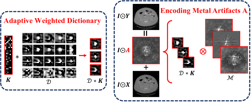
Figure 1: The proposed weighted convolutional dictionary model for encoding metal artifacts $\bm{A}$ as $\left(\mathcal{D}\ast\bm{K}\right)\otimes\mathcal{M}$. Here the dictionary $\mathcal{D}$ is sample-invariant and the weighting coefficient $\bm{K}$ is sample-variant. By updating $\bm{K}$, the representation kernel for artifacts (i.e., $\mathcal{D}\ast\bm{K}$) can be adaptively inferred for every input image $\bm{Y}$.

With the rapid development of deep learning (DL), recent years have witnessed the promising progress of DL for the MAR task. Some early works adopted convolutional neural network (CNN) to reconstruct clean sinograms and then utilized the filtered-back-projection transformation to reconstruct the artifact-reduced CT images Zhang and Yu (2018); Ghani and Karl (2019). Later, researchers adopted different learning strategies, e.g., residual learning Huang et al. (2018) and adversarial learning Wang et al. (2018), to directly learn the artifact-reduced CT images. Very recently, there is a new research line for the MAR task, which focuses on the mutual learning of sinograms and CT images Lin et al. (2019); Lyu et al. (2020); Wang et al. (2021b, c).

Attributed to the powerful learning ability of CNN, deep MAR methods generally achieve superior performance over conventional model-based approaches. Yet, there is still some room for further performance improvement. First, most of current deep MAR works pay less attention to exploring the intrinsic prior knowledge of the specific MAR task, such as non-local streaking structures of metal artifacts (see Fig. 1). The explicit embedding of such prior information can assist to regularize the solution space for metal artifact extraction, and further boost the MAR performance of deep networks as well as its generalization ability. Second, the involved image enhancement modules in current deep MAR works Lin et al. (2019); Lyu et al. (2020) are roughly the variants of U-Net. With such a general network design, the physical interpretability of every network module is unclear.

In this paper, we propose an explicit model to encode the prior observations underlying the MAR task and fully embed it into an adaptive convolutional dictionary network (namely ACDNet). The proposed framework inherits the clear interpretability of model-based methods and maintains the powerful representation ability of learning-based methods. In summary, our main contributions can be concluded as:

1) Prior Formulation. For the MAR task, we explore that artifacts in different metal-corrupted CT images always present common (i.e., sample-invariant) patterns, such as non-local repetitive streaking structures, but with the specific (i.e., sample-invariant) intensity variation in CT images. Based on such prior observations, we adaptively encode the artifacts in every metal-corrupted CT image as a weighted convolutional dictionary (WCD) model (see Fig. 1).

2) Prior Embedding and Interpretability. To solve the WCD model, we propose an iterative algorithm with only simple operators and easily construct the ACDNet by unfolding every iterative step into the corresponding network module. Similar to learning-based methods, ACDNet automatically learns the priors for artifact-free CT images in a purely data-driven manner, overcoming the disadvantages of hand-crafted priors. Similar to model-based methods, ACDNet is explicitly integrated with the WCD model of artifacts and has clear physical interpretability corresponding to our optimization algorithm. The proposed ACDNet thus integrates the advantages of model-based and learning-based methodologies.

3) Fine Generalization. With the regularization of the explicit WCD model, ACDNet can more accurately extract artifacts complying with prior structures. Comprehensive experiments, including cross-body-site generalization and synthesis-to-clinical generalization, finely substantiate the superiority of our method as well as excellent computation efficiency. Especially, as an image-domain-based method without utilizing sinogram, our ACDNet can be adopted as a plug-in module, which is easily integrated into current computer-aided diagnosis systems to deal with some practical scenarios where the projection data is difficult to acquire.

2 Methodology

In this section, we propose an explicit model to adaptively encode the priors of every metal-affected CT image and derive a simple algorithm for the subsequent network design.

2.1 Weighted Convolutional Dictionary Model

For an observed metal-corrupted CT image $\bm{Y}$, it is composed of two regions, i.e., metal part and non-metal part. Since metals generally have higher CT values than normal tissues, we ignore the information in the metal region and make efforts to reconstruct the non-metal region of $\bm{Y}$. Therefore, the decomposition model can be derived as:

$$\bm{I}\odot\bm{Y}=\bm{I}\odot\bm{X}+\bm{I}\odot\bm{A},$$ (1)

where $\bm{I}$ is a binary non-metal mask; $\bm{X}\in\mathbb{R}^{H\times W}$ is the to-be-estimated clean CT image; $\bm{A}$ is the to-be-extracted metal artifacts; $\odot$ is an element-wise multiplication.

From Eq. (1), the estimation of $\bm{X}$ and $\bm{A}$ from $\bm{Y}$ is an ill-posed inverse problem. Against this issue, most of current learning-based methods empirically design complicated network architectures to directly learn $\bm{X}$ from $\bm{Y}$, which lack the consideration of explicit prior knowledge of MAR (e.g., the patterns of metal artifacts). However, embedding the explicit prior is helpful to finely regularize the solution space of such an ill-posed problem, and thus further improves the performance of deep networks, especially generalization ability. Based on this motivation, we explore the specific prior structures underlying the MAR task, and then propose a strategy to explicitly embed them into deep networks.

Prior Formulation.

Specifically, we disclose that for different metal-affected CT images, the metal artifacts are with roughly common patterns, e.g., non-local repetitive streaking structures. Besides, due to the mutual influence between normal tissues and metal artifacts, the patterns of metal artifacts in different CT images are not exactly the same and generally have some specific characteristics, e.g., pixel intensities of metal artifacts vary between different metal-corrupted CT images. Based on these prior observations, we formulate a weighted convolutional dictionary (WCD) model to encode the metal artifacts $\bm{A}$ as Wang et al. (2021d):

$$\bm{A}=\sum_{n=1}^{N}\left(\mathcal{D}\ast\bm{K}_{n}\right)\otimes\bm{M}_{n}=\left(\mathcal{D}\ast\bm{K}\right)\otimes\mathcal{M},$$ (2)

where $\mathcal{D}\in\mathbb{R}^{p\times p\times d}$ is a sample-invariant dictionary (i.e., a set of convolutional filters) representing common local patterns of metal artifacts in different metal-corrupted CT images; $\bm{K}_{n}\in\mathbb{R}^{d}$ is a sample-wise weighting coefficient to learn the specific convolutional filter for $\bm{A}$ by computing $\mathcal{D}\ast\bm{K}_{n}$ as $\sum^{d}_{i=1}\mathcal{D}[:,:,i]\odot\bm{K}_{n}[i]$ (see Fig. 1); $\bm{M}_{n}\in\mathbb{R}^{H\times W}$ is the coefficients representing the locations for the local patterns of metal artifacts; $p$ is the size of convolutional filters; $d$ is the total number of filters in the dictionary $\mathcal{D}$; $N$ is the actual number of filters encoding the artifacts $\bm{A}$; and the $\otimes$ between $\left(\mathcal{D}\ast\bm{K}\right)$ and $\mathcal{M}$ is a convolutional operation in tensor form. Specifically, $\left(\mathcal{D}\ast\bm{K}_{n}\right)\in\mathbb{R}^{p\times p}$, $\bm{K}\in\mathbb{R}^{d\times N}$, $\left(\mathcal{D}\ast\bm{K}\right)\in\mathbb{R}^{p\times p\times N}$, $\mathcal{M}\in\mathbb{R}^{H\times W\times N}$, and

$$\small\begin{split}&\bm{K}=\left[\bm{K}_{1},\bm{K}_{2},\cdots,\bm{K}_{N}\right],~{}~{}\mathcal{M}=\left[\bm{M}_{1},\bm{M}_{2},\cdots,\bm{M}_{N}\right],\\ &\mathcal{D}\ast\bm{K}=\left[\mathcal{D}\ast\bm{K}_{1},\mathcal{D}\ast\bm{K}_{2},\cdots,\mathcal{D}\ast\bm{K}_{N}\right].\end{split}$$ (3)

Note that convolutional dictionary model has been verified to be applicable to represent repetitive patterns by existing studies Wang et al. (2021a). Compared to these methods, the proposed weighted mechanism in Eq. (2) has two main merits for the MAR task: 1) It delivers not only the sample-invariant/common knowledge, but also the sample-wise characteristics for information embedding, which can adaptively encode the prior structure for every CT image; 2) With such a weighted convolutional dictionary, we can choose an $N$ smaller than $d$, which further shrinks the solution space for estimating $\bm{A}$ and thereby improves the model generalization (see Sec. 4).

By substituting Eq. (2) into Eq. (1), we can derive:

$$\bm{I}\odot\bm{Y}=\bm{I}\odot\bm{X}+\bm{I}\odot\left(\left(\mathcal{D}\ast\bm{K}\right)\otimes\mathcal{M}\right).$$ (4)

As shown, our goal is to estimate the sample-wise $\bm{K}$, $\mathcal{M}$, and $\bm{X}$ from $\bm{Y}$. Note that the non-metal mask $\bm{I}$ is pre-known (see Sec. 4) and the common dictionary $\mathcal{D}$ can be automatically learnt from training data (see Sec. 3). With the maximum-a-posterior framework, the optimization problem is:

$$\begin{split}\min_{{\bm{K},\mathcal{M},\bm{X}}}&\left\|\bm{I}\odot\left(\bm{Y}\!-\!\bm{X}\!-\!\left(\mathcal{D}\ast\bm{K}\right)\!\otimes\!\mathcal{M}\right)\right\|_{F}^{2}\\ &~{}~{}+\alpha f_{1}(\bm{K})\!+\beta f_{2}(\mathcal{M})\!+\!\gamma f_{3}(\bm{X})\\ &\text{subject to}~{}~{}~{}\left\|\bm{K}_{n}\right\|_{2}=1,n=1,2,\ldots,N,\end{split}$$ (5)

where $f_{1}\left(\cdot\right)$, $f_{2}\left(\cdot\right)$, and $f_{3}\left(\cdot\right)$ are regularization functions, delivering the prior knowledge of $\bm{K}$, $\mathcal{M}$, and $\bm{X}$, respectively; $\alpha$, $\beta$, and $\gamma$ are regularization weights.

2.2 Optimization Algorithm

Traditional solvers for the problem (1) often involve complex Fourier and inverse Fourier transforms, which are difficult to integrate into deep networks. In this regard, we design a new optimization algorithm with only simple operators. Concretely, the proximal gradient technique Beck and Teboulle (2009) is adopted to alternately update $\bm{K}$, $\mathcal{M}$, and $\bm{X}$:

Solving $\bm{K}$:

From the problem (1), at the $(t+1)$-th iteration, $\bm{K}$ is solved as follows:

$$\small\begin{split}&\bm{K}^{(t+1)}\!=\!\underset{{\bm{K}}}{\text{argmin}}\left\|\bm{I}\!\odot\!\left(\bm{Y}\!\!-\!\!\bm{X}^{(t)}\!\!-\!\!\left(\mathcal{D}\ast\bm{K}\right)\otimes\mathcal{M}^{(t)}\right)\right\|_{F}^{2}\!\!+\!\alpha f_{1}(\bm{K}),\\ &\text{subject to}~{}~{}~{}\left\|\bm{K}_{n}\right\|_{2}=1,n=1,2,\ldots,N,\end{split}$$ (6)

and the quadratic approximation Beck and Teboulle (2009) of the objective function in the problem (6) is:

$$\begin{split}\bm{K}^{(t+1)}&=\underset{\bm{K}\in\Omega}{\text{argmin}}~{}~{}~{}g_{1}\left(\bm{K}^{(t)}\!\right)+\frac{1}{2\eta_{1}}\left\|\bm{K}-\bm{K}^{(t)}\right\|_{F}^{2}\\ &\hskip 8.53581pt+\left\langle\bm{K}-\bm{K}^{(t)},\nabla g_{1}\left(\bm{K}^{(t)}\!\right)\right\rangle+\alpha f_{1}\left(\bm{K}\right),\end{split}$$ (7)

where $\Omega=\{\bm{K}|\left\|\bm{K}_{n}\right\|_{2}=1,n=1,2,\cdots,N\}$; $g_{1}\left(\bm{K}^{(t)}\right)=\!\left\|\bm{I}\odot\left(\bm{Y}\!-\!\bm{X}^{(t)}\!-\left(\mathcal{D}\ast\bm{K}^{(t)}\right)\!\otimes\!\mathcal{M}^{(t)}\right)\right\|_{F}^{2}$; $\eta_{1}$ is the stepsize. Hence, we can get the following equation:

$$\small\begin{split}&\frac{\partial g_{1}\left(\bm{K}^{(t)}\right)}{\partial\bm{K}_{n}}\!=\!\left(\!U^{f}_{3}\!\left(\!\mathcal{D}\otimes^{d}\bm{M}_{n}^{(t)}\right)\!\right)\!\\ &\quad\quad\quad\text{vec}\!\left(\bm{I}\odot\left(\left(\mathcal{D}\ast\bm{K}^{(t)}\right)\otimes\mathcal{M}^{(t)}\!+\!\bm{X}^{(t)}\!-\!\bm{Y}\right)\right),\end{split}$$ (8)

where $\otimes^{d}$ is the depth-wise convolutional computation; $U^{f}_{3}(\cdot)$ denotes the unfolding operation at the $3^{rd}$ mode; and vec($\cdot$) denotes the vectorization.

Clearly, Eq. (7) can be equivalently written as:

$$\small\bm{K}^{(t+1)}=\underset{\bm{K}\in\Omega}{\text{argmin}}\frac{1}{2}\left\|\bm{K}\!-\!\!\left(\!\bm{K}^{(t)}\!\!-\!\eta_{1}\nabla g_{1}\left(\bm{K}^{(t)}\right)\!\right)\right\|_{F}^{2}\!+\alpha\eta_{1}f_{1}\left(\bm{K}\right).$$ (9)

For general prior $f_{1}(\cdot)$ Donoho (1995), Eq. (9) is derived as:

$$\bm{K}^{(t+1)}=\mbox{prox}_{\alpha\eta_{1}}\!\!\left(\bm{K}^{(t+0.5)}\right),$$ (10)

where $\bm{K}^{(t+0.5)}=\bm{K}^{(t)}-\eta_{1}\nabla g_{1}\left(\bm{K}^{(t)}\right)$; $\nabla g_{1}\left(\bm{K}^{(t)}\right)\!\!=\!\!\left[\!\frac{\partial g_{1}\left(\bm{K}^{(t)}\right)}{\partial\bm{K}_{1}},\frac{\partial g_{1}\left(\bm{K}^{(t)}\right)}{\partial\bm{K}_{2}},\ldots,\frac{\partial g_{1}\left(\bm{K}^{(t)}\right)}{\partial\bm{K}_{N}}\!\right]$; $\mbox{prox}_{\alpha\eta_{1}}\left(\cdot\right)$ is a proximal operator which is related to $f_{1}\left(\cdot\right)$. The constraint space $\Omega$ can be achieved by introducing a normalization operation into $\mbox{prox}_{\alpha\eta_{1}}\left(\cdot\right)$ (see Sec. 3).

Solving $\mathcal{M}$:

Similarly, at the $(t+1)$-th iteration, $\mathcal{M}$ can be updated by solving the quadratic approximation of the subproblem with respect to $\mathcal{M}$ as:

$$\small\begin{split}\mathcal{M}^{(t+1)}=\underset{\mathcal{M}}{\text{argmin}}&\frac{1}{2}\left\|\mathcal{M}-\left(\!\mathcal{M}^{(t)}-\eta_{2}\nabla g_{2}\left(\mathcal{M}^{(t)}\right)\right)\right\|_{F}^{2}\\ &\vspace{6mm}+\beta\eta_{2}f_{2}\left(\mathcal{M}\right),\end{split}$$ (11)

where $\eta_{2}$ is the stepsize and $g_{2}\left(\mathcal{M}^{(t)}\right)\!=\!\left\|\bm{I}\odot\left(\bm{Y}\!-\!\bm{X}^{(t)}\!-\!\left(\mathcal{D}\ast\bm{K}^{(t+1)}\right)\!\otimes\!\mathcal{M}^{(t)}\right)\right\|_{F}^{2}$. Similarly, the solution of problem (11) is deduced as:

$$\mathcal{M}^{(t+1)}=\mbox{prox}_{\beta\eta_{2}}\left(\mathcal{M}^{(t+0.5)}\right),$$ (12)

where $\mbox{prox}_{\beta\eta_{2}}(\cdot)$ is a proximal operator related to the regularization function $f_{2}(\cdot)$ about $\mathcal{M}$; $\mathcal{M}^{(t+0.5)}=\mathcal{M}^{(t)}\!-\!\eta_{2}\nabla g_{2}\left(\mathcal{M}^{(t)}\right)$; $\nabla g_{2}\left(\mathcal{M}^{(t)}\right)=\left(\mathcal{D}\ast\bm{K}^{(t+1)}\right)\otimes^{T}\!\left(\bm{I}\odot\left(\left(\mathcal{D}\ast\bm{K}^{(t+1)}\right)\otimes\mathcal{M}^{(t)}\!+\!\bm{X}^{(t)}\!-\!\bm{Y}\right)\right)$; and $\otimes^{T}$ is the transposed convolution operation.

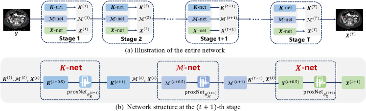
Figure 2: (a) The proposed ACDNet consists of $T$ stages. (b) The detailed structure at any stage where $\bm{K}^{(t+1)}$, $\mathcal{M}^{(t+1)}$, and $\bm{X}^{(t+1)}$ are successively updated by $\bm{K}$-net, $\mathcal{M}$-net, and $\bm{X}$-net, respectively, based on Eqs. (10), (12), and (14).

Solving $\bm{X}$:

Given $\bm{K}^{(t+1)}$ and $\mathcal{M}^{(t+1)}$, the quadratic approximation of the subproblem about $\bm{X}$ is derived as:

$$\bm{X}^{(t+1)}\!=\!\underset{\bm{X}}{\text{argmin}}\frac{1}{2}\!\left\|\bm{X}\!-\!\left(\!\bm{X}^{(t)}\!-\!\eta_{3}\nabla g_{3}\left(\bm{X}^{(t)}\right)\!\right)\right\|_{F}^{2}\!\!+\!\gamma\eta_{3}f_{3}\!\left(\bm{X}\right),$$ (13)

where $g_{3}\left(\!\bm{X}^{(t)}\!\right)\!=\!\left\|\bm{I}\!\odot\!\left(\!\bm{Y}\!\!-\!\!\bm{X}^{(t)}\!\!-\!\!\left(\mathcal{D}\!\ast\!\bm{K}^{(t+1)}\right)\!\otimes\!\mathcal{M}^{(t+1)}\right)\!\right\|_{F}^{2}$. Then, the updating rule of $\bm{X}$ is written as:

$$\bm{X}^{(t+1)}=\mbox{prox}_{\gamma\eta_{3}}\left(\bm{X}^{(t+0.5)}\right),$$ (14)

where $\bm{X}^{(t+0.5)}\!=\!\left(\bm{1}\!-\!\eta_{3}\bm{I}\right)\odot\bm{X}^{(t)}+\eta_{3}\bm{I}\odot\left(\!\bm{Y}\!\!-\!\!\left(\mathcal{D}\ast\bm{K}^{(t+1)}\right)\!\otimes\!\mathcal{M}^{(t+1)}\!\right)$; $\mbox{prox}_{\gamma\eta_{3}}(\cdot)$ is dependent on the prior function $f_{3}(\cdot)$ about $\bm{X}$.

Eqs. (10), (12), and (14) constitute the entire iterative process for solving the problem (1). As seen, the proposed algorithm only contains simple operators, which makes it easier to accordingly build the deep network framework upon the algorithm. Note that $\mbox{prox}_{\alpha\eta_{1}}(\cdot)$, $\mbox{prox}_{\beta\eta_{2}}(\cdot)$, and $\mbox{prox}_{\gamma\eta_{3}}(\cdot)$ are implicit operators, which are automatically learnt from training data by virtue of the powerful prior fitting capability of deep networks. This manner has been fully used and widely validated to be effective and helpful to explore interpretable knowledge by recent studies (e.g.. Wang et al. (2021d); Xie et al. (2019)). The details are in Sec. 3.

3 Network Design and Analysis

Due to the specific design of joint model-driven (i.e., prior knowledge) and data-driven (i.e., deep networks) frameworks, deep unfolding techniques have achieved great success in computer vision tasks, such as single image rain removal Wang et al. (2021d) and low-light image enhancement Liu et al. (2022). Inspired by this, we specifically design an adaptive convolutional dictionary network (ACDNet) for the MAR task by unfolding the iterative algorithm in Sec. 2.2 into the corresponding network structure.

Fig. 1 (a) displays the entire network structure with $T$ stages, which correspond to $T$ iterations of the optimization algorithm in Sec. 2.2. For every stage, our network consists of three sub-nets, i.e., $\bm{K}$-net, $\mathcal{M}$-net, and $\bm{X}$-net corresponding to addressing the three subproblems, i.e.,, solving $\bm{K}$, $\mathcal{M}$, and $\bm{X}$, respectively. Fig. 1 (b) shows the detailed network connections at every stage, which are constructed by sequentially unfolding the iterative rules, i.e., Eq. (10), Eq. (12), and Eq. (14), respectively. With the unfolding operations, every network module corresponds to the specific iterative step of the proposed optimization algorithm. Thus, the entire network framework has a clear physical interpretability. Next we present the information of sub-nets in detail:

$\bm{K}$-net:

At the $(t+1)$-th stage, $\bm{K}^{(t+0.5)}$ is computed and fed to $\text{proxNet}_{\theta_{\bm{K}}^{(t+1)}}(\cdot)$ to execute the operator $\mbox{prox}_{\alpha\eta_{1}}(\cdot)$. Then, the updated weighting coefficient is: $\bm{K}^{(t+1)}=\text{proxNet}_{\theta_{\bm{K}}^{(t+1)}}\left(\bm{K}^{(t+0.5)}\right)$, where $\text{proxNet}_{\theta_{\bm{K}}^{(t+1)}}(\cdot)$ is a residual structure, i.e., [Linear+ReLU+Linear+Skip Connection+Normalization at the dimension $d$].

$\mathcal{M}$-net:

Given $\bm{K}^{(t+1)}$, $\mathcal{M}^{(t)}$, and $\bm{X}^{(t)}$, we can compute $\mathcal{M}^{(t+1)}=\text{proxNet}_{\theta_{\mathcal{M}}^{(t+1)}}\left(\mathcal{M}^{(t+0.5)}\right)$, where $\text{proxNet}_{\theta_{\mathcal{M}}^{(t+1)}}(\cdot)$ is the unfolding form of $\mbox{prox}_{\beta\eta_{2}}(\cdot)$—ResNet with three [Conv+BN+ReLU+Conv+BN+Skip Connection] residual blocks.

$\bm{X}$-net:

Similarly, given $\bm{K}^{(t+1)}$, $\mathcal{M}^{(t+1)}$, and $\bm{X}^{(t)}$, the artifact-reduced CT image can be updated by $\bm{X}^{(t+1)}=\mbox{proxNet}_{\theta_{\bm{X}}^{(t+1)}}\left(\bm{X}^{(t+0.5)}\right)$, where $\text{proxNet}_{\theta_{\bm{X}}^{(t+1)}}(\cdot)$ has the same network structure to $\text{proxNet}_{\theta_{\mathcal{M}}^{(t+1)}}(\cdot)$.

With $T$-stage optimization, we can get the final CT image $\bm{X}^{(T)}$. All the involved parameters are $\{\theta_{\bm{K}}^{(t)},\theta_{\mathcal{M}}^{(t)},\theta_{\bm{X}}^{(t)}\}_{t=1}^{T}$, $\{\eta_{i}\}_{i=1}^{3}$, and the common dictionary $\mathcal{D}$. They can be automatically learnt from training samples in an end-to-end manner. Note that $\mathcal{D}$ is achieved by a common convolutional layer. More details, including the initialization ($\bm{K}^{(0)}$, $\mathcal{M}^{(0)}$, $\bm{X}^{(0)}$), are given in Supplemental Material (SM).

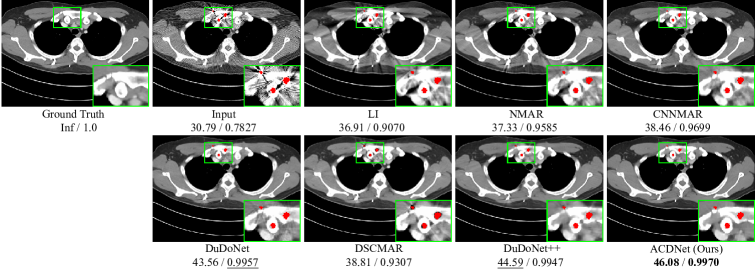
Figure 3: Performance comparison of different MAR approaches on a metal-corrupted CT image selected from the synthesized DeepLesion data. PSNR (dB)/SSIM below is for reference. The red pixels stand for metallic implants.

Methods	Large Metal     $\longrightarrow$      Small Metal					Average
Input	24.12/0.6761	26.13/0.7471	27.75/0.7659	28.53/0.7964	28.78/0.8076	27.06/0.7586
LI Kalender et al. (1987)	27.21/0.8920	28.31/0.9185	29.86/0.9464	30.40/0.9555	30.57/0.9608	29.27/0.9347
NMAR Meyer et al. (2010)	27.66/0.9114	28.81/0.9373	29.69/0.9465	30.44/0.9591	30.79/0.9669	29.48/0.9442
CNNMAR Zhang and Yu (2018)	28.92/0.9433	29.89/0.9588	30.84/0.9706	31.11/0.9743	31.14/0.9752	30.38/0.9644
DuDoNet Lin et al. (2019)	29.87/0.9723	30.60/0.9786	31.46/0.9839	31.85/0.9858	31.91/0.9862	31.14/0.9814
DSCMAR Yu et al. (2020)	34.04/0.9343	33.10/0.9362	33.37/0.9384	32.75/0.9393	32.77/0.9395	33.21/0.9375
DuDoNet++ Lyu et al. (2020)	36.17/0.9784	38.34/0.9891	40.32/0.9913	41.56/0.9919	42.08/0.9921	39.69/0.9886
ACDNet (Ours)	37.91/0.9872	39.30/0.9920	41.14/0.9949	42.43/0.9961	42.64/0.9965	40.68/0.9933

Table 1: Average PSNR (dB)/SSIM of different MAR methods on the synthesized DeepLesion data.

ProxNet:

Following recent great deep unfolding-based works Wang et al. (2021b); Xie et al. (2019), we also set proximal operator with ResNet. Although it is very hard to inversely derive the form of regularizer by integrating ResNet function due to its complicated form, but as has comprehensively substantiated by previous research, it does be helpful to explore insightful structural prior. Besides, adopting such learning-based manner to automatically learn implicit regularizers is more flexible, avoiding hand-crafted prior design.

Interpretability:

Unlike most of current deep MAR networks, which are heuristically built based on the off-the-shelf network blocks, ACDNet is naturally constructed under the guidance of the optimization algorithm with careful data fidelity term design. In this regard, the entire network integrates the interpretability of model-based methods. Besides, such interpretability is visually validated by Fig. 3 of SM.

Remark:

Deep unfolding technique is a general tool for network design. To apply it, the key challenge is how to elaborately design model and optimization algorithm to make it work for specific applications. For the MAR task, we have specifically made some substantial ameliorations: 1) The adaptive prior of artifacts is incorporated into data fidelity term which can finely guide the network learning and boost the generalization ability; 2) Unlike other solvers with complicated computations (e.g., Fourier transformation and matrix inversion), the proposed optimization algorithm is elaborately designed which only contains simple operators and makes the unfolding process easy and proper; 3) Compared to current popular dual-domain MAR methods, ACDNet only uses CT image domain data, which is more friendly to practical applications where the projection data is difficult to acquire. Besides, ACDNet can be easily integrated into current computer-aided diagnosis systems as a plug-in module.

Loss Function.

With supervision on the extracted artifact $\bm{A}^{(t)}$ and CT image $\bm{X}^{(t)}$ at every stage, the training loss is:

$$\small\begin{split}\mathcal{L}&\!=\!\!\sum_{t=0}^{T}\mu_{t}\bm{I}\!\odot\!\left\|\bm{X}\!\!-\!\!\bm{X}^{(t)}\right\|_{F}^{2}\!\!+\!\omega_{1}\!\left(\sum_{t=0}^{T}\mu_{t}\bm{I}\!\odot\!\left\|\bm{X}\!\!-\!\!\bm{X}^{(t)}\right\|_{1}\!\right)\\ &+\omega_{2}\left(\sum_{t=0}^{T}\mu_{t}\bm{I}\odot\left\|\bm{Y}-\bm{X}-\bm{A}^{(t)}\right\|_{1}\right),\end{split}$$ (15)

where $\bm{X}$ is the clean (i.e., ground truth) CT image. In all experiments, $\mu_{T}$ is set to 1; $\mu_{t}\,\,\,(t=0,1,\cdots,T-1)$ is 0.1; $\omega_{1}$ and $\omega_{2}$ are empirically set to $5\times 10^{-4}$.

Implementation Details.

ACDNet is optimized through Adam optimizer based on PyTorch. The framework is trained on an NVIDIA Tesla V100-SMX2 GPU with a batch size of 32. The initial learning rate is $2\times 10^{-4}$ and divided by 2 at epochs [50, 100, 150, 200]. The total number of epochs is 300. The size of input image patch is $64\times 64$ pixels and it is randomly flipped horizontally and vertically. More explanations are included in SM.

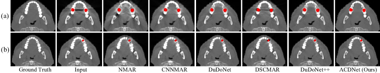
Figure 4: Generalization results. Artifact-reduced results on the synthesized dental CT images with different metallic implants.

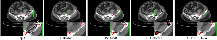
Figure 5: Generalization results. Performance comparison on a real clinical metal-affected CT image from CLINIC-metal.

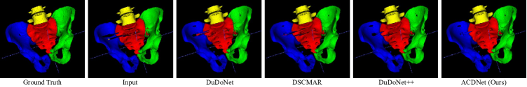
Figure 6: Downstream segmentation results of an artifact-reduced CLINIC-metal volume reconstructed by different MAR approaches.

4 Experiments

In this section, we conduct extensive experiments to validate the effectiveness of our method.

4.1 Dataset & Experimental Setting

Synthesized Data. Following the simulation procedure in Yu et al. (2020), we randomly choose 1,200 clean CT images from the public DeepLesion dataset Yan et al. (2018) and collect 100 metal masks from Zhang and Yu (2018) to synthesize the paired clean/metal-corrupted CT images. Specifically, 90 metals together with 1000 clean CT images for training and 10 ones together with the remaining 200 clean CT images for testing. Similar to Lin et al. (2019); Lyu et al. (2020), we sequentially take every two testing metal masks as one group for performance evaluation. In addition, to evaluate the cross-body-site generalization performance, clean dental CT images Yu et al. (2020) are adopted and the corresponding metal-corrupted images are generated under the same simulation protocol on DeepLesion.

Clinical Data. A public clinical dataset, i.e., CLINIC-metal Liu et al. (2021), which contains 14 metal-corrupted volumes with pixel-wise annotations of multiple bone structures (i.e., sacrum, left hip, right hip, and lumbar spine), is used for evaluation. Following Yu et al. (2020), the clinical metal masks are segmented with thresholding of 2500 HU.

Baselines. Representative MAR methods are used, including traditional LI Kalender et al. (1987) and NMAR Meyer et al. (2010), learning-based CNNMAR Zhang and Yu (2018), DuDoNet Lin et al. (2019), DSCMAR Yu et al. (2020), and DuDoNet++ Lyu et al. (2020).

Evaluation Metric. We adopt the PSNR/SSIM for quantitative comparison on synthesized data and only visual comparison on clinical data due to the lack of clean CT images.

4.2 Performance Evaluation

DeepLesion Data.

Fig. 3 presents the visual comparison on an image from synthesized metal-corrupted DeepLesion. As shown, our approach significantly removes the artifacts and finely recovers evident details. The average PSNR/SSIM scores on the entire DeepLesion dataset are listed in Table 1. It can be observed that ACDNet consistently achieves the best scores with varying sizes of metallic implants.

Dental Data.

Fig. 4 shows the MAR visual results on the synthesized dental CT images with different metallic implants, where deep MAR methods are trained on the synthesized DeepLesion (focusing on abdomen and thorax) and directly tested on the dental CT images. Due to the regularization with the explicit WCD model, ACDNet can more accurately identify the artifacts and accomplish the better reconstruction of artifact-reduced CT images. The results show the excellent cross-body-site generalizability of our method.

Clinical Data.

Fig. 7 presents the MAR comparison of generalization results on a clinical metal-corrupted CT image. Our ACDNet finely preserves more bone structures and removes more artifacts. Fig. 8 displays the downstream segmentation results of an artifact-reduced CLINIC-metal volume, which are reconstructed by different MAR approaches. The proposed ACDNet is significantly superior to other approaches, which reveals its excellent potential for clinical applications. Due to the limited space, we only provide the results of the latest MAR methods.

Methods	#Parameters	Testing Time
DuDoNet Lin et al. (2019)	25,834,251	0.4225
DSCMAR Yu et al. (2020)	25,834,251	0.3638
DuDoNet++ Lyu et al. (2020)	25,983,627	0.8062
ACDNet (Ours)	1,602,809	0.3138

Table 2: The number of network parameters and average testing time (seconds) computed on 2000 images with size $416\times 416$ pixels on an NVIDIA Tesla V100-SMX2 GPU.

Computation Efficiency.

Table 2 reports that our method has fewer network parameters (i.e., storage cost) and computation consumption, compared to other methods.

5 Conclusion and Future Work

In this paper, for the MAR task, we have proposed a weighted convolutional dictionary model to explicitly and adaptively encode the structural prior of metal artifacts for every input image. Then, by unfolding a simple-yet-effective optimization algorithm, we have easily built the deep network, which integrated the advantages of both model-based methods and learning-based methods. Experiments executed on three public datasets verified the excellent generalizability and excellent computational efficiency of our method.

Following current state-of-the-art (SOTA) MAR methods, we adopt the thresholding manner to simply segment the metal for clinical data. An unsatisfactory threshold possibly makes tissues be wrongly regarded as metals and most MAR methods would fail to recover image details. Although our method consistently achieve good performances for different sizes of metals and show the robustness, as a direction to further boost the performance of our framework, the joint optimization of automated metal localization and MAR is worthwhile to further explore. Besides, like SOTA MAR methods, we process CT images slice by slice for fairness. It would be very meaningful to do 3D prior modeling for the MAR task.

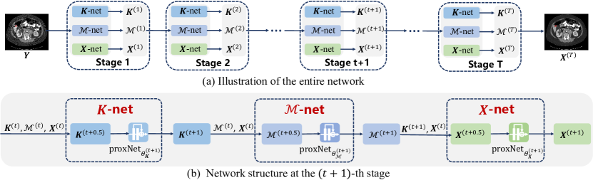
Figure 1: (a) The proposed network architecture consists of $T$ stages. At every stage, it is sequentially composed of $\bm{K}$-net, $\mathcal{M}$-net, and $\bm{X}$-net. (b) The detailed structure at any stage where $\bm{K}^{(t+1)}$, $\mathcal{M}^{(t+1)}$, and $\bm{X}^{(t+1)}$ are successively updated by $\bm{K}$-net, $\mathcal{M}$-net, and $\bm{X}$-net, respectively, based on the iterative algorithm as Eqs. (10), (12), and (14) of the main text.

Supplementary Material

Appendix A More Details about Network Structure

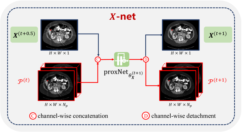
Figure 2: During the network implementation, this channel expansion operation is implemented for $\bm{X}$-net in Fig. 1.

A.1 Channel Expansion

The proposed network framework is shown in Fig. 1 where $\bm{X}^{(T)}$ is the final reconstructed CT image. From the $\bm{X}$-net, the original input of the proximal network $\text{proxNet}_{\theta_{\bm{X}}^{(t+1)}}(\cdot)$ is $\bm{X}^{(t+0.5)}$ with only one gray channel. For the effective feature extraction and the better reconstruction of artifact-reduced CT image, we introduce a channel expansion operation during network implementation, as shown in Fig. 2. Specifically, $\mathcal{P}^{(t)}$ is an auxiliary variable for channel expansion, which is updated together with $\bm{X}^{(t+0.5)}$. Hence, the updated input of $\text{proxNet}_{\theta_{\bm{X}}^{(t+1)}}(\cdot)$ consists of $(1+N_{p})$ channels (by the channel-wise concatenation). In all our experiments, $N_{p}=32$. Correspondingly, for the output of $\text{proxNet}_{\theta_{\bm{X}}^{(t+1)}}(\cdot)$, we execute the channel-wise detachment operation to obtain the updated $\bm{X}^{(t+1)}$ and $\mathcal{P}^{(t)}$.

A.2 Initialization

From Fig. 1 and Fig. 2, to proceed the iterative reconstruction process, we need to initialize $\bm{K}^{(0)}$, $\mathcal{M}^{(0)}$, $\mathcal{P}^{(0)}$, and $\bm{X}^{(0)}$. Since only the metal-corrupted CT image $\bm{Y}$ is accessible, we can directly initialize $\mathcal{P}^{(0)}$ and $\bm{X}^{(0)}$ and then utilize them to initialize $\bm{K}^{(0)}$ and $\mathcal{M}^{(0)}$.

Initializing $\mathcal{P}^{(0)}$ and $\bm{X}^{(0)}$.

Motivated by the aforementioned channel expansion, we can first execute the channel-wise concatenation between $\bm{X}_{LI}$ and $\mathcal{C}_{p}\otimes\bm{X}_{LI}$, and feed the concatenated result to the deep network $\text{proxNet}_{\theta_{\bm{X}}^{(0)}}(\cdot)$. Then, with the channel-wise detachment operation, we can easily obtain the $\mathcal{P}^{(0)}$ and $\bm{X}^{(0)}$. Here $\bm{X}_{LI}$ is the resorted CT image by the conventional linear interpolation (LI) based method Kalender et al. [1987]; $\mathcal{C}_{p}$ is a common convolutionl layer where the size of convolutional kernel is $k\times k\times 1\times N_{p}$ (in our experiment, the value is set to $3\times 3\times 1\times 32$); $\mbox{proxNet}_{\theta_{\bm{X}}^{(0)}}(\cdot)$ is a ResNet, with the same structure to $\mbox{proxNet}_{\theta_{\bm{X}}^{(t)}}(\cdot)$ as described in Sec. 3 of the main text.

Initializing $\bm{K}^{(0)}$ and $\mathcal{M}^{(0)}$.

From Fig. 1, it is observed that only with $\mathcal{P}^{(0)}$ and $\bm{X}^{(0)}$, we still cannot execute the initialization $\bm{K}^{(0)}$ and $\mathcal{M}^{(0)}$. To solve the problem, we first disentangle $\mathcal{M}$ and $\bm{K}$ for the initialization of $\mathcal{M}^{(0)}$. Then, with $\mathcal{M}^{(0)}$, $\mathcal{P}^{(0)}$, and $\bm{X}^{(0)}$, we can easily get the $\bm{K}^{(0)}$.

Specifically, the original optimization problem is

$$\begin{split}\min_{{\bm{K},\mathcal{M},\bm{X}}}&\left\|\bm{I}\odot\left(\bm{Y}\!-\!\bm{X}\!-\!\left(\mathcal{D}\ast\bm{K}\right)\!\otimes\!\mathcal{M}\right)\right\|_{F}^{2}\\ &~{}~{}+\alpha f_{1}(\bm{K})\!+\beta f_{2}(\mathcal{M})\!+\!\gamma f_{3}(\bm{X})\\ &\text{subject to}~{}~{}~{}\left\|\bm{K}_{n}\right\|_{2}=1,n=1,2,\ldots,N,\end{split}$$ (1)

where $\mathcal{D}\in\mathbb{R}^{p\times p\times d}$; $\bm{K}\in\mathbb{R}^{d\times N}$; and $\mathcal{M}\in\mathbb{R}^{H\times W\times N}$. In our experiments, $p=9$, $d=32$, and $N=6$.

To disentangle $\mathcal{M}$ and $\bm{K}$, we ignore the weighting mechanism and then simplify the problem  (1) as:

$$\min_{{\mathcal{M},\bm{X}}}\left\|\bm{I}\odot\left(\bm{Y}\!-\!\bm{X}\!-\!\mathcal{D}\!\otimes\!\mathcal{M}\right)\right\|_{F}^{2}+\beta f_{2}(\mathcal{M})\!+\!\gamma f_{3}(\bm{X}),$$ (2)

note that in this simplified case, $d=N=32$.

By adopting the similar solution process in Sec. 3 of the main text and executing the corresponding unfolding operation upon the derived algorithm, we can construct the deep unfolding sub-networks for solving the problem (2). The network computations are sequentially composed of:

$$\mathcal{M}^{(t+1)}=\text{proxNet}_{\theta_{\mathcal{M}}^{(t+1)}}\left(\mathcal{M}^{(t+0.5)}\right),$$ (3)

$$\bm{X}^{(t+1)}=\mbox{proxNet}_{\theta_{\bm{X}}^{(t+1)}}\left(\bm{X}^{(t+0.5)}\right),$$ (4)

where

$$\mathcal{M}^{(t+0.5)}=\mathcal{M}^{(t)}\!-\!\eta_{2}\mathcal{D}\otimes^{T}\!\left(\bm{I}\odot\left(\mathcal{D}\otimes\mathcal{M}^{(t)}\!+\!\bm{X}^{(t)}\!-\!\bm{Y}\right)\right),$$ (5)

$$\bm{X}^{(t+0.5)}\!=\!\left(\bm{1}\!-\!\eta_{3}\bm{I}\right)\odot\bm{X}^{(t)}+\eta_{3}\bm{I}\odot\left(\!\bm{Y}\!\!-\!\!\mathcal{D}\!\otimes\!\mathcal{M}^{(t+1)}\!\right).$$ (6)

Based on Eq. (3) and the aforementioned $\bm{X}^{(0)}$, we can get the initial estimation of $\mathcal{M}^{(0)}$. Note that, for a better initialization, we further execute an extra iteration sequentially consisting of Eqs. (3) (4) to refine the $\mathcal{M}^{(0)}$ and $\bm{X}^{(0)}$.

With $\mathcal{M}^{(0)}$, $\mathcal{P}^{(0)}$, and $\bm{X}^{(0)}$, based on the original computations involved in $\bm{K}$-net, i.e., $\bm{K}^{(t+1)}=\text{proxNet}_{\theta_{\bm{K}}^{(t+1)}}\left(\bm{K}^{(t+0.5)}\right)$ (see Sec. 3 of the main text), we can get the initialization of $\bm{K}^{(0)}$. Note that in our experiments, the initialization $\mathcal{M}^{(0)}$ obtained by Eq. (3) for the simplified problem (2) has 32 channels. To execute the regular iterative computation for the original problem  (1), we simply select the first six channels as $\mathcal{M}^{(0)}$ for $\mathcal{M}$-net shown in Fig. 1.

Appendix B More Details about Data Simulation

Following the simulation protocol in Yu et al. [2020], we synthesize the paired metal-free/metal-corrupted CT images by randomly choosing 1,200 clean CT images from the DeepLesion dataset (mainly focusing on abdomen and thorax) Yan et al. [2018] and collecting 100 metal masks with diverse types from Zhang and Yu [2018]. During the synthesis of metal-affected CT images, we consider different factors, including poly-chromatic X-ray, partial volume effect, beam hardening, and Poisson noise, which follow the existing studies Zhang and Yu [2018]; Liao et al. [2019]; Lin et al. [2019]; Yu et al. [2020]; Lyu et al. [2020]. 640 projection views are uniformly spaced between 0-360 degrees. The size of the synthesized CT images is $416\times 416$ pixels and the size of the corresponding sinogram data is $641\times 640$ pixels.

Algorithm 1 Training ACDNet for MAR

0: $\bm{K}^{(0)}$, $\mathcal{M}^{(0)}$, $\bm{X}^{(0)}$, training data $\left\{\bm{\bm{Y}}_{n},\bm{\bm{X}}_{n},\bm{\bm{I}}_{n}\right\}_{n=1}^{N}$, batch size, patch size, initial learning rate

0: Network parameters $\{\theta_{\bm{K}}^{(t)},\theta_{\mathcal{M}}^{(t)},\theta_{\bm{X}}^{(t)}\}_{t=1}^{T}$, stepsizes $\{\eta_{i}\}_{i=1}^{3}$, and the common dictionary $\mathcal{D}$

1: while The loss in Eq. (15) of main text is not convergent do

2:    for $t=0$ to $T-1$ do

3:       $\bm{K}$-net:   $\bm{K}^{(t+1)}=\text{proxNet}_{\theta_{\bm{K}}^{(t+1)}}\left(\bm{K}^{(t+0.5)}\right)$

4:       $\mathcal{M}$-net:  $\mathcal{M}^{(t+1)}=\text{proxNet}_{\theta_{\mathcal{M}}^{(t+1)}}\left(\mathcal{M}^{(t+0.5)}\right)$

5:       $\bm{X}$-net:   $\bm{X}^{(t+1)}=\mbox{proxNet}_{\theta_{\bm{X}}^{(t+1)}}\left(\bm{X}^{(t+0.5)}\right)$

6:    end for

7:    Update ACDNet (i.e., $T$-stage $\bm{K}$-net, $\mathcal{M}$-net, and $\bm{X}$-net).

8: end while

Appendix C More Implementation Details

The training process is listed as Algorithm 1. We execute two testing tasks on CLINIC-metal, including metal artifact reduction (MAR) task and the downstream pelvic fracture segmentation task. For the segmentation task, we first need to train a U-Net on clean pelvic data. The training details are described as:

A publicly available clinical metal-free dataset–CLINIC Liu et al. [2021], with the annotations of multi-bone structures, is adopted. It consists of 103 clean volumes (35,518 slices). The Adam optimizer Kingma and Ba [2014] is adopted for network optimization. The initial learning rate is $2\times 10^{-4}$ and divided by 2 every 20 epochs. The network converges after 42 epochs of training with the batch size of 12. The total loss function is the combination of cross-entropy loss and dice loss.

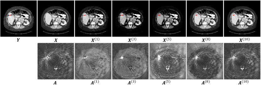
Figure 3: Visualization of artifact-reduced image $\bm{X}^{(t)}$ and artifact $\bm{A}^{(t)}$ extracted by our ACDNet at the stage $t$. The total stage $T$ is 10 and $\bm{A}$ is the groudtruth artifact, expressed as $\left(\bm{Y}-\bm{X}\right)\odot\bm{I}$.

Appendix D More Analysis about ACDNet

D.1 Interpretability Verification

To verify the specific interpretability of our proposed ACDNet for the MAR task, we visualize the learning process, as shown in Fig. 3. It is easily observed that with the increase of iterative stage $t$, the extracted artifact layer $\bm{A}^{(t)}$ is approaching the ground truth artrifact $\bm{A}$ and the reconstructed CT image $\bm{X}^{(t)}$ is approaching the ground truth clean image $\bm{X}$. This results finely substantiate that the mutual promotion learning of $\bm{K}$-net, $\bm{M}$-net, and $\bm{X}$-net and the guidance of the explicit weighted prior model make the entire network framework optimize in a right direction for accurately identifying metal artifacts. Such interpretable learning process is the intrinsic characteristic of our iterative optimization framework. Actually, compared to heuristic network designs, our ACDNet is more transparent and interpretable since every network module is accordingly built based on the optimization algorithm.

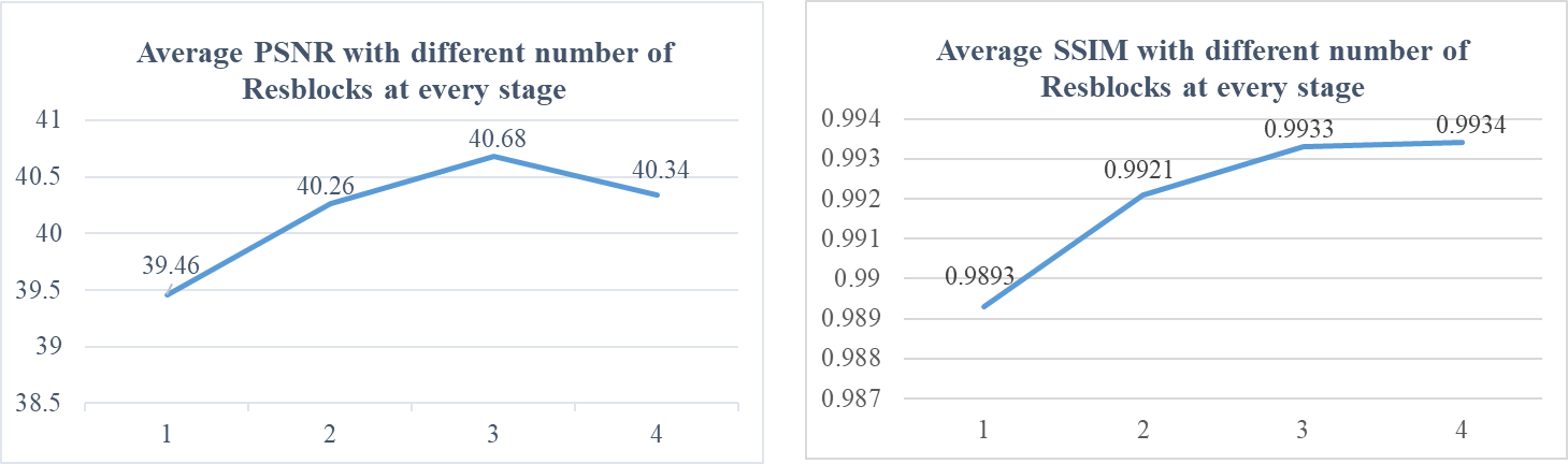
Figure 4: The average PSNR/SSIM of our method on the synthesized DeepLesion dataset with the different numbers of Resblocks involved in deep proximal networks $\text{proxNet}_{\theta_{\bm{X}}^{(t)}}(\cdot)$.

D.2 Ablation Study

The number of Resblocks.

Fig. 4 shows the variation on MAR performance of our framework with the different numbers of Resblocks in deep proximal networks $\text{proxNet}_{\theta_{\bm{X}}^{(t)}}(\cdot)$ at every stage, where the total number $T$ of iterative stages is 10. Note that $\text{proxNet}_{\theta_{\mathcal{M}}^{(t)}}(\cdot)$ adopts the same number of Resblocks to $\text{proxNet}_{\theta_{\bm{X}}^{(t)}}(\cdot)$. Based on the results, we adopt 3 Resblocks to construct the backbone of deep proximal networks as described in Sec. 3 of the main text. Note that we only adopt 1 Resblock for building $\text{proxNet}_{\theta_{\bm{K}}^{(t)}}(\cdot)$ to reduce the network parameters of the whole framework.

The Updating Order.

Optimization order	PSNR (dB)
$\bm{K}$-net, $\mathcal{M}$-net, $\bm{X}$-net	40.68
$\mathcal{M}$-net, $\bm{K}$-net, $\bm{X}$-net	40.42
$\bm{K}$-net, $\bm{X}$-net, $\mathcal{M}$-net	40.54
$\mathcal{M}$-net, $\bm{X}$-net, $\bm{K}$-net	40.35
$\bm{X}$-net, $\bm{K}$-net, $\mathcal{M}$-net	40.24
$\bm{X}$-net, $\mathcal{M}$-net, $\bm{K}$-net	40.64

Table 1: Average PSNR on synthesized DeepLesion under different updating orders.

Table 1 lists the performance of our proposed ACDNet with different updating orders. As seen, our method is insensitive to the order.

Appendix E More Experiments

E.1 Performance Comparisons

DeepLesion Data.

We provide more visual results of different MAR approaches on different metallic implants with varying sizes as shown in Fig. 5 and Fig. 6. It is clear that, among the comparing methods, the proposed framework achieves the better reconstruction results.

Dental Data.

Table 2 reports the quantitative performance of different MAR methods on the synthesized dental CT images shown in Fig. 4 of main text. As seen, it shows the excellent cross-body-site generalizability of our method.

Figure	Input	LI	NMAR	CNNMAR	DuDoNet	DSCMAR	DuDoNet++	ACDNet (Ours)
(a)	34.52/0.8839	31.14/0.8783	31.69/0.9003	35.23/0.9532	35.67/0.9685	36.80/0.9709	36.04/0.9857	41.41/0.9903
(b)	36.46/0.9282	33.93/0.9435	34.86/0.9626	36.37/0.9761	39.38/0.9744	37.11/0.9806	40.71/0.9903	45.40/0.9954

Table 2: PSNR (dB)/SSIM of different MAR methods on the synthesized dental CT images shown in Fig.4 of main text.

Bone	Input	LI	NMAR	CNNMAR	DuDoNet	DSCMAR	DuDoNet++	Ours
Sacrum	92.47	90.86	91.51	92.44	93.26	92.52	93.50	94.34
Left hip	95.43	93.91	94.27	94.85	96.11	95.33	96.17	96.75
Right hip	87.47	91.23	91.68	92.50	93.89	93.22	93.79	94.98
Lumbar spine	94.43	94.53	94.64	94.89	95.51	94.75	95.64	95.77
Average DC	92.45	92.63	93.03	93.67	94.69	93.96	94.77	95.46

Table 3: The average Dice coefficient (DC) (%) results on the clinical downstream segmentation task.

Clinical Data.

Fig. 7 presents the visual comparison of MAR performance on a clinical image selected from CLINIC-metal, where deep MAR methods are trained on synthesized DeepLesion data.

Table 3 reports the average segmentation accuracy on 14 artifact-removed CLINIC-metal volumes. Please note that this segmentation task is very challenging due to the large gap between DeepLesion and clinical pelvic CT. Then the quantitative improvement for a new method is generally not that significant, like the gain (0.08) of DuDoNet++ over DuDoNet. Thus, the looking-like “small” improvement (0.69) of our method over DuDoNet++ is rational to support its effectiveness. Actually, visual comparison should be more intuitive. Fig. 8 displays the downstream segmentation results of an artifact-reduced CLINIC-metal volume, which are reconstructed by different MAR approaches. This more intuitively shows clinical benefits of our method.

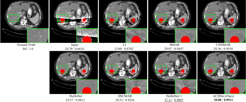
Figure 5: Performance comparison of different MAR approaches on a metal-corrupted CT image with large metals selected from the synthesized DeepLesion data. PSNR (dB)/SSIM below is listed for reference. The red pixels stand for metallic implants.

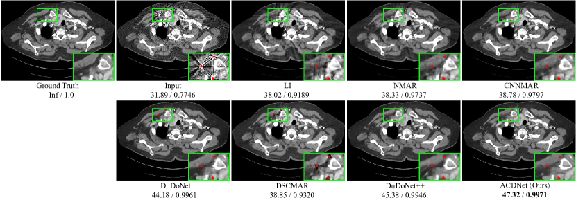
Figure 6: Performance comparison of different MAR approaches on a metal-corrupted CT image with small metals selected from the synthesized DeepLesion data. PSNR (dB)/SSIM below is listed for reference.

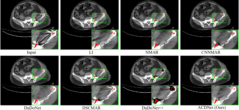
Figure 7: Generalization results. Performance comparison on a real clinical metal-affected CT image from CLINIC-metal, where deep MAR methods are trained on the synthesized DeepLesion data. The red pixels stand for metallic implants.

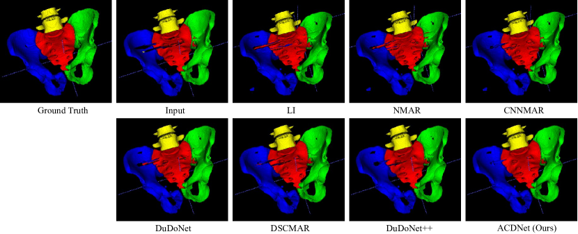
Figure 8: Downstream segmentation results of an artifact-reduced CLINIC-metal volume, which are reconstructed by different MAR approaches. Note that the deep MAR methods are trained on the synthesized DeepLesion data.

Table	CNNMAR	DuDoNet	DSCMAR	DuDoNet++	Ours
Table 1∗	$<0.001$	$<0.001$	$<0.001$	$<0.001$	n.a
Table 2	0.0421	0.0147	0.0391	0.0362	n.a
Table 3	$<0.001$	$<0.001$	$<0.001$	0.0203	n.a

Table 4: P-values comparison. Note that Table 1 is the one in the main text.

P-values Analysis.

With the paired t-test, the P-values for the quantitative comparisons listed in Table 1 of main text, Table 2, and Table 3 are reported in Table 4. It is easily observed that all P-values are less than the significance level 0.05. Thus, our method performs significantly better.

References

- Beck and Teboulle [2009] Amir Beck and Marc Teboulle. A fast iterative shrinkage-thresholding algorithm for linear inverse problems. SIAM Journal on Imaging Sciences, 2(1):183–202, 2009.
- Donoho [1995] David L Donoho. De-noising by soft-thresholding. IEEE Transactions on Information Theory, 41(3):613–627, 1995.
- Ghani and Karl [2019] Muhammad Usman Ghani and W Clem Karl. Fast enhanced CT metal artifact reduction using data domain deep learning. IEEE Transactions on Computational Imaging, 6:181–193, 2019.
- Huang et al. [2018] Xia Huang, Jian Wang, Fan Tang, Tao Zhong, and Yu Zhang. Metal artifact reduction on cervical CT images by deep residual learning. Biomedical Engineering Online, 17(1):1–15, 2018.
- Kalender et al. [1987] Willi A Kalender, Robert Hebel, and Johannes Ebersberger. Reduction of CT artifacts caused by metallic implants. Radiology, 164(2):576–577, 1987.
- Kingma and Ba [2014] Diederik P Kingma and Jimmy Ba. Adam: A method for stochastic optimization. arXiv preprint arXiv:1412.6980, 2014.
- Lemmens et al. [2008] Catherine Lemmens, David Faul, and Johan Nuyts. Suppression of metal artifacts in CT using a reconstruction procedure that combines MAP and projection completion. IEEE Transactions on Medical Imaging, 28(2):250–260, 2008.
- Liao et al. [2019] Haofu Liao, Wei-An Lin, S Kevin Zhou, and Jiebo Luo. ADN: Artifact disentanglement network for unsupervised metal artifact reduction. IEEE Transactions on Medical Imaging, 39(3):634–643, 2019.
- Lin et al. [2019] Wei-An Lin, Haofu Liao, Cheng Peng, Xiaohang Sun, Jingdan Zhang, Jiebo Luo, Rama Chellappa, and Shaohua Kevin Zhou. DuDoNet: Dual domain network for CT metal artifact reduction. In Proceedings of the IEEE/CVF Conference on Computer Vision and Pattern Recognition, pages 10512–10521, 2019.
- Liu et al. [2021] Pengbo Liu, Hu Han, Yuanqi Du, Heqin Zhu, Yinhao Li, Feng Gu, Honghu Xiao, Jun Li, Chunpeng Zhao, Li Xiao, et al. Deep learning to segment pelvic bones: large-scale CT datasets and baseline models. International Journal of Computer Assisted Radiology and Surgery, 16(5):749–756, 2021.
- Liu et al. [2022] Xinyi Liu, Qi Xie, Qian Zhao, Hong Wang, and Deyu Meng. Low-light image enhancement by retinex based algorithm unrolling and adjustment. arXiv preprint arXiv:2202.05972, 2022.
- Lyu et al. [2020] Yuanyuan Lyu, Wei-An Lin, Haofu Liao, Jingjing Lu, and S Kevin Zhou. Encoding metal mask projection for metal artifact reduction in computed tomography. In International Conference on Medical Image Computing and Computer Assisted Intervention, pages 147–157, 2020.
- Meyer et al. [2010] Esther Meyer, Rainer Raupach, Michael Lell, Bernhard Schmidt, and Marc Kachelrieß. Normalized metal artifact reduction (NMAR) in computed tomography. Medical Physics, 37(10):5482–5493, 2010.
- Wang et al. [2018] Jianing Wang, Yiyuan Zhao, Jack H Noble, and Benoit M Dawant. Conditional generative adversarial networks for metal artifact reduction in CT images of the ear. In International Conference on Medical Image Computing and Computer Assisted Intervention, pages 3–11, 2018.
- Wang et al. [2021a] Hong Wang, Yuexiang Li, Nanjun He, Kai Ma, Deyu Meng, and Yefeng Zheng. DICDNet: Deep interpretable convolutional dictionary network for metal artifact reduction in CT images. IEEE Transactions on Medical Imaging, 2021.
- Wang et al. [2021b] Hong Wang, Yuexiang Li, Haimiao Zhang, Jiawei Chen, Kai Ma, Deyu Meng, and Yefeng Zheng. InDuDoNet: An interpretable dual domain network for CT metal artifact reduction. In International Conference on Medical Image Computing and Computer-Assisted Intervention, pages 107–118, 2021.
- Wang et al. [2021c] Hong Wang, Yuexiang Li, Haimiao Zhang, Deyu Meng, and Yefeng Zheng. InDuDoNet+: A model-driven interpretable dual domain network for metal artifact reduction in CT images. arXiv preprint arXiv:2112.12660, 2021.
- Wang et al. [2021d] Hong Wang, Qi Xie, Qian Zhao, Yong Liang, and Deyu Meng. RCDNet: An interpretable rain convolutional dictionary network for single image deraining. arXiv preprint arXiv:2107.06808, 2021.
- Xie et al. [2019] Qi Xie, Minghao Zhou, Qian Zhao, Deyu Meng, Wangmeng Zuo, and Zongben Xu. Multispectral and hyperspectral image fusion by MS/HS fusion net. In Proceedings of the IEEE/CVF Conference on Computer Vision and Pattern Recognition, pages 1585–1594, 2019.
- Yan et al. [2018] Ke Yan, Xiaosong Wang, Le Lu, Ling Zhang, Adam P Harrison, Mohammadhadi Bagheri, and Ronald M Summers. Deep lesion graphs in the wild: Relationship learning and organization of significant radiology image findings in a diverse large-scale lesion database. In Proceedings of the IEEE Conference on Computer Vision and Pattern Recognition, pages 9261–9270, 2018.
- Yu et al. [2020] Lequan Yu, Zhicheng Zhang, Xiaomeng Li, and Lei Xing. Deep sinogram completion with image prior for metal artifact reduction in CT images. IEEE Transactions on Medical Imaging, 40(1):228–238, 2020.
- Zhang and Yu [2018] Yanbo Zhang and Hengyong Yu. Convolutional neural network based metal artifact reduction in X-ray computed tomography. IEEE Transactions on Medical Imaging, 37(6):1370–1381, 2018.
- Zhang et al. [2011] Xiaomeng Zhang, Jing Wang, and Lei Xing. Metal artifact reduction in X-ray computed tomography (CT) by constrained optimization. Medical Physics, 38(2):701–711, 2011.