Mechanism of Roll-Streak Structure Formation and Maintenance in Turbulent Shear Flow

Abstract

In wall-bounded shear flow the primary coherent structure is the streamwise roll and streak (R-S). Absent of an associated instability the R-S has been ascribed to non-normality mediated interaction between the mean flow and perturbations. This interaction may occur either directly due to excitation of a transiently growing perturbation or indirectly due to destabilization of the R-S by turbulent Reynolds stresses. A fundamental distinction between the direct and the indirect mechanisms, which is central to understanding the physics of turbulence, is that in the direct mechanism the R-S is itself the growing structure while in the indirect mechanism the R-S emerges as a self-organized structure. In the emergent R-S theory the fundamental mechanism is organization by the streak of Reynolds stresses configured to support its associated roll by the lift-up process. This requires that a streak organizes turbulent perturbations such as to produce Reynolds stresses configured to reinforce the streak. In this paper we provide detailed analysis explaining physically why this positive feedback occurs and is a universal property of turbulence in shear flow. DNS data from the same turbulent flow as that used in the theoretical study (Poisseullle flow at $R=1650$) is also analyzed verifying that this mechanism operates in DNS.

1 Introduction

While advances in experiment, simulation and theory continue to be made, the physical mechanisms underlying turbulence in shear flows remains incompletely understood. The problem of shear flow turbulence can be divided into two components: transition from the laminar to the turbulent state and maintenance of the turbulent state. The transition problem is posed by the lack of an inflection in the velocity profiles of boundary layer flows. Inflections are associated by the Rayleigh theorem with existence of robust instabilities that continue in viscous flows from the inflectional instability of the same velocity profile in an inviscid flow. The problem of robust disturbance growth in perturbation stable shear flows was solved when it was recognized that the non-normality of the underlying linear dynamics allows perturbation growth in the absence of exponential instability. The concept of transient growth in shear flow has roots in the classical work of Kelvin and Orr (Kelvin, 1887; Orr, 1907). Although three dimensional perturbations in the form of a roll-streak structure were observed in boundary layers (Townsend, 1956; Klebanoff et al., 1962; Kline et al., 1967; Blackwelder & Eckelmann, 1979; Robinson, 1991) and related to the nonmodal lift-up growth mechanism (Landahl, 1980), comprehensive observational evidence for the mechanism of nonmodal growth in boundary layer flows awaited the advent of DNS at Reynolds numbers ${\cal O}(1000)$, for which turbulence is maintained, and particle image velocimetry (PIV) of turbulent shear flows. The methods of non-normal operator analysis and optimal perturbation theory were first applied in the context of laboratory shear flows to two dimensional disturbances (Farrell, 1988). It was believed at the time that secondary instability of finite amplitude two dimensional equilibria were the mechanism of transition (Pierrehumbert, 1986; Bayly et al., 1988) and it was shown that these unstable two dimensional nonlinear finite amplitude equilibria could be readily excited by even very small optimal initial perturbations (Butler & Farrell, 1994). However, it became increasingly apparent from observation and simulation that the finite amplitude structures associated with transition are three dimensional and analysis of three dimensional optimal perturbation growth followed (Butler & Farrell, 1992, 1993; Farrell & Ioannou, 1993a, b; Reddy & Henningson, 1993; Trefethen et al., 1993; Schmid & Henningson, 2001). These analyses revealed that the optimally growing three dimensional structure is associated with cross-stream/spanwise rolls and associated streamwise streaks and is related to the linear lift up mechanism. The remarkable convected coordinate solutions for perturbation growth in unbounded shear flow (Kelvin, 1887) allow closed form solution for the scale independent structures producing optimal growth in three dimensional shear flow (Farrell & Ioannou, 1993a, b). These closed form optimal solutions in unbounded shear flow confirm the result found numerically in bounded shear flows that for sufficiently long optimizing times streamwise rolls produce optimal energy growth while for short optimizing times the optimal perturbations are oblique wave structures that synergistically exploit both the two dimensional shear and the three dimensional lift up mechanisms producing vortex cores oriented at an angle of approximately $60$ degrees from the spanwise direction. And indeed, the roll-streak and oblique accompanying structure complex that is predicted to produce optimal growth by analysis of non-normal perturbation dynamics of shear flows has been convincingly seen in both observations and simulations (Klebanoff et al., 1962; Schoppa & Hussain, 2000; Adrian, 2007; Wu & Moin, 2009; Jiménez, 2013) and shown to be essentially related to the non-normality of shear flow dynamics (Kim & Lim, 2000; Schoppa & Hussain, 2002).

The most direct mechanism exploiting non-normality to form roll-streak (R-S) structures is to introduce an optimal perturbation into the flow, perhaps by using a trip or other device (Butler & Farrell, 1992; Reddy & Henningson, 1993; Trefethen et al., 1993). A related approach is to stochastically force the flow which can be analyzed using stochastic turbulence modeling (STM) (Farrell & Ioannou, 1993d, c, 1994, 1998a, 1998b; Bamieh & Dahleh, 2001; Jovanović & Bamieh, 2005; Hoepffner & Brandt, 2008). Because of the non-normal nature of perturbation growth in shear flow, stochastic turbulence models are closely related to optimal perturbation dynamics. In conventional stochastic turbulence models the R-S is envisioned to arise from chance occurrence of optimal or near optimal perturbations in the stochastic forcing (Bamieh & Dahleh, 2001; Hwang & Cossu, 2010a, b; McKeon & Sharma, 2010). These mechanisms exploit the linear non-normal growth process directly. Although the R-S structures could arise from an optimal or near optimal perturbation occurring by chance in the free stream or instigated by a mechanism such as a trip or a boundary injection, the ubiquity of the R-S structure in shear at low levels of free stream turbulence (Adrian, 2007; Wu & Moin, 2009) suggests a more systematic origin and a number of ideas have been advanced to explain the continuous generation and maintenance of this structure in turbulent shear flow (Schoppa & Hussain, 2002; Panton, 2001). However, the ubiquity of streak formation suggests, as argued by Schoppa & Hussain (2000), that some form of instability process underlies the formation of streaks and that this instability involves an intrinsic association between the R-S structure and associated oblique waves. Such a three dimensional instability must differ qualitatively from the familiar laminar shear flow instability given that it would necessarily violate the Squire theorem and that extensive search had failed to reveal a candidate instability in the linearized Navier-Stokes equations. Nevertheless, its existence was frequently inferred from experiment and simulation e.g. Andersson et al. (1999) who concluded that the evidence “..corresponds to some fundamental mode triggered in the flat-plate boundary layer when subjected to high enough levels of free-stream turbulence..”. Efforts to identify the mechanism underlying instability of the R-S structure include exponential instability mechanisms (Brown & Thomas, 1977) and the Craik-Leibovich instability (Phillips et al., 1996). Proposed algebraic growth mechanisms involve a streamwise average torque produced by interaction of discrete oblique waves (Benney, 1960; Jang et al., 1986).

In a study of a turbulent shear flow Hamilton et al. (1995) noted that the Reynolds stresses arising from turbulent perturbations were systematically correlated with the R-S so as to maintain the roll in the manner of a feedback process referred to as the self-sustaining process (SSP). This correlation was subsequently attributed to the structure of the Reynolds stresses produced by inflectionsl instability of the streak (Waleffe, 1997), modal critical layer fluxes (Hall & Smith, 1991; Hall & Sherwin, 2010) and transiently growing structures (Schoppa & Hussain, 2002). However, suppression of unstable modes has been demonstrated to have essentially no effect on maintenance of the R-S providing a constructive proof that inflectional instability is not responsible for the SSP (Farrell & Ioannou, 2012a; Lozano-Durán et al., 2021). This left collocation of transiently growing structures as being responsible for providing the roll maintaining torques as suggested by Schoppa & Hussain (2002). The central physical problem posed by this result is explaining how the perturbation Reynolds stresses are maintained by non-normal growth processes to have the correct amplitude and structure to provide the roll collocated torques required by the instability of the pre-transitional boundary layer R-S as well as the time dependent R-S of the SSP in the turbulent state.

The cross stream-spanwise roll structure provides a powerful mechanism for forming streamwise streaks in shear flows when continuously forced by an oblique wave structure. However, observation of the spatial correlation of perturbation structures in turbulent flow does not support the existence of extensive interfering oblique plane waves. Nevertheless, if we observe a turbulent shear flow in the cross stream-spanwise plane at a fixed streamwise location we see that at any instant there is a substantial torque from Reynolds stress divergence forcing cross stream-spanwise rolls. The problem is that this torque is not systematic and so it vanishes in temporal or streamwise average. However, in the presence of a perturbation streak the symmetry in the spanwise direction is broken and the torque from Reynolds stress divergence can become organized to produce the positive feedback between the streak and roll required to destabilize this structure by continuously and coherently exploiting the powerful non-normal R-S amplification mechanism. The existence of this mechanism for destabilizing the R-S in turbulence makes it likely that some dynamical perturbation complex exists to exploit it. That this is so was demonstrated by deriving from the Navier-Stokes equations a system of statistical state dynamics (SSD) equations closed at second order, eigenanalysis of which reveals the instability responsible for destabilizing turbulent shear flow to streak formation (Farrell & Ioannou, 2012a; Farrell et al., 2017b). This fundamental instability underlying shear flow turbulence had evaded detection in part because it has no counterpart in the linearized Navier-Stokes equations.

This emergent instability can be understood as a streak formation mechanism in which background turbulence, rather than itself comprising the perturbation the non-normal growth of which constitutes the streak, instead the stochastically occurring perturbations are organized and collocated by the streak to form optimally growing structures with oblique wave form that force the cross stream-spanwise roll by inducing a Reynolds stress torque linearly proportional to streak amplitude and collocated with the streak resulting in an emergent exponential instability of the combined roll-streak-turbulence complex.

It has been demonstrated constructively using second order SSD analysis of the N-S equations that a dynamical perturbation complex exploiting the high non-normality of the R-S plus turbulence complex exists to destabilize the pre-transitional boundary layer forming a modal R-S and that this mechanism persists subsequent to transition to maintain the temporally fluctuating R-S complex in the fully turbulent state through a parametric instabiity (Farrell & Ioannou, 2012a; Farrell et al., 2017b). However, the specific mean R-S components and their supporting perturbation structures as well as the origin and the mechanism by which these structures produce torques correctly collocated to explain the ubiquitous occurrence of the mean R-S in wall-bounded shear flow turbulence remains to be fully elucidated and its predictions tested against DNS data. In this work we analyze the mechanism by which turbulent perturbations are organized by streaks to force and maintain the R-S and compare with DNS to verify that the Reynolds stress destabilization mechanism occurs and is consistent with the observed formation and maintenance of the R-S structure in turbulent Poiseuille flow.

2 Analysis of the forces responsible for the formation and maintenance of streamwise-mean rolls

The flow velocity is decomposed into streamwise mean, denoted by $\mathbf{U}=(U,V,W)$, with $U$ being the mean streamwise velocity, in the $x$ streamwise direction; $V$ the mean cross stream velocity in the $y$ cross-stream direction; and $W$ the mean spanwise velocity in the spanwise $z$ direction. The velocity deviations from the mean, are $\mathbf{u}=(u,v,w)$, and referred to as the perturbations. The non-dimensionalized equations governing the mean and the perturbations flow and pressure fields $(P,p)$ in a channel take the form

$$\partial_{t}\mathbf{U} +\mathbf{U}\bm{\cdot}\bm{\nabla}\mathbf{U}+\nabla P-R^{-1}\Delta\mathbf{U}=-\overline{\mathbf{u}\bm{\cdot}\bm{\nabla}\mathbf{u}}~{},$$ (1a)

$$\partial_{t}\mathbf{u} +\mathbf{U}\bm{\cdot}\bm{\nabla}\mathbf{u}+\mathbf{u}\bm{\cdot}\bm{\nabla}\mathbf{U}+\bm{\nabla}p-R^{-1}\Delta\mathbf{u}=-(\mathbf{u}\bm{\cdot}\bm{\nabla}\mathbf{u}-\overline{\mathbf{u}\bm{\cdot}\bm{\nabla}\mathbf{u}})~{}.$$ (1b)

$$\bm{\nabla}\bm{\cdot}\mathbf{U}=0~{},~{}~{}~{}\bm{\nabla}\bm{\cdot}\mathbf{u}=0~{},$$ (1c)

with no slip boundary conditions at the channel walls. The overline denotes the streamwise average and $R$ is the Reynolds number of the flow. In the equation for the mean (1a) $-\overline{\mathbf{u}\bm{\cdot}\bm{\nabla}\mathbf{u}}$ represents the Reynolds stress induced forcing of the mean by the perturbations. Assuming unit density we do not insist on the nomenclature distinction between force and acceleration so that divergence of the Reynolds stress induces a streamwise mean force per unit mass in Eq. (1a), which is independent of $x$, resulting in streamwise velocity component acceleration

$$F_{x}=-\partial_{y}(\overline{uv})-\partial_{z}(\overline{uw})~{},$$ (2)

and cross-stream and spanwise velocity component accelerations:

$$F_{y}=-\partial_{z}(\overline{vw})-\partial_{y}(\overline{v^{2}})~{}~{},~{}F_{z}=-\partial_{y}(\overline{vw})-\partial_{z}(\overline{w^{2}})~{}.$$ (3)

We want to examine the maintenance of the streamwise mean roll circulation with velocity components $V$, $W$ and streamwise mean vorticity $\Omega_{x}=\partial_{y}W-\partial_{z}V$. From (1a) we obtain that $\Omega_{x}$ is governed by:

$$\frac{D\Omega_{x}}{Dt}=G_{x}+\frac{1}{R}\Delta_{2}\Omega_{x}~{},$$ (4)

with $D/Dt=\partial_{t}+V\partial_{y}+W\partial_{z}$ the substantial derivative of the streamwise vorticity under advection by the streamwise mean flow $(V,W)$. On the RHS of Eq. (4) appears the dissipation term, with the notation $\Delta_{2}=\partial_{y}^{2}+\partial_{z}^{2}$ for the two-dimensional Laplacian, and the Reynolds stress roll vorticity forcing term arising from the turbulent perturbations

$$G_{x}=\partial_{y}F_{z}-\partial_{z}F_{y}=\left(\partial_{z}^{2}-\partial_{y}^{2}\right)\overline{vw}+\partial_{yz}\left(\overline{v^{2}}-\overline{w^{2}}\right)~{}.$$ (5)

In the absence of $G_{x}$ the mean streamwise vorticity decays as it then obeys the advection-diffusion equation

$$\frac{D\Omega_{x}}{Dt}=\frac{1}{R}\Delta_{2}\Omega_{x}~{},$$ (6)

which implies

$$\frac{d}{dt}\int\Omega_{x}^{2}dydz=-\frac{1}{R}\int|\bm{\nabla}\Omega_{x}|^{2}dydz~{}~{},~{}\frac{d}{dt}\int(V^{2}+W^{2})dydz=-\frac{1}{R}\int\Omega_{x}^{2}dydz~{},$$ (7)

indicating decay in time of both the square vorticity, $\int\Omega_{x}^{2}dydz$, and the energy of the roll circulation $\int(V^{2}+W^{2})dydz$, as noted by Moffatt (1990). This diagnostic clearly implies that the formation and maintenance of the streamwise mean roll requires a systematic source of streamwise mean vorticity that can only be provided by the rotational component of the Reynolds stress vorticity forcing $G_{x}$. In wall-bounded flows with cross-stream mean flow shear such rolls would lead to formation by the lift-up process of low and high speed spanwise inhomogeneities in the mean streamwise flow, $U$, referred to as streaks. This streak component is defined as $U_{s}=U-[U]_{z}$ where $[U]_{z}$ is the spanwise average of $U$. These considerations require that a Reynolds stress torque exists to maintain a streamwise roll circulation and that a properly collocated streamwise roll necessarily forces a collocated streak so that the R-S is a dynamical consequence of a streamwise mean Reynolds stress torque. The dynamical hypothesis of the SSP (Hamilton et al., 1995; Waleffe, 1997) is that the streak instigates the torque that maintains both the roll and the streak itself through the lift-up process. If this is so then explaining how the streak gives rise to its self-sustaining roll-inducing torque is the central dynamical problem posed by the maintenance of wall-bounded turbulence. Given that the torques are not dependent on modal instability (Farrell & Ioannou, 2012a) theoretical explanation of this SSP requires identifying how transiently growing structures produce the required torque.

In order to understand the mechanism of roll formation by perturbation Reynolds stress we must first isolate the component of $\bm{F}=(F_{y},F_{z})$ responsible for forcing the roll circulation. It is clear from (5) that only the rotational part of $\bm{F}$ is involved in roll formation, the substantial part of $\bm{F}$ that is divergent being cancelled by the immediate development of the pressure field required by continuity. The force $\bm{f}$ that remains from $\bm{F}$ to induce the roll circulation is obtained by a Helmholtz-Hodge decomposition of the total Reynolds stress force $\bm{F}$ into a divergent component, -$\bm{\nabla}\varphi$, which acts as a pressure force, and a non-divergent component $\bm{f}=(f_{y},f_{z})$, so that:

$$\bm{F}=\bm{f}-\bm{\nabla}\varphi~{},$$ (8)

and $f_{y}=0$ at the boundaries of the channel. This Helmholtz-Hodge decomposition in the channel domain is unique (Chorin & Marsden, 1997). The non-divergent force field $\bm{f}$ has components

$$\bm{f}=-\Delta_{2}^{-1}(\bm{\nabla}\times G_{x}\widehat{\mathbf{x}})]~{},§$$ (9)

where $\widehat{\mathbf{x}}$ is the unit vector in the streamwise direction, and $\Delta_{2}^{-1}$ the inverse of the two-dimensional Laplacian $\Delta_{2}=\partial_{yy}+\partial_{zz}$, rendered unique by the boundary conditions. The force-field $\bm{f}=(f_{y},f_{z})$ determines the roll circulation, as it is the force-field that accelerates the $(V,W)$ velocity field by:

$$\partial_{t}V=f_{y}=-\Delta^{-1}_{2}\partial_{z}G_{x}~{}~{},~{}~{}\partial_{t}W=f_{z}=\Delta^{-1}_{2}\partial_{y}G_{x}~{}~{}.$$ (10)

3 Properties of turbulent perturbation Reynolds stress in mean flows without streaks

Consider a perturbation field $\mathbf{u}$ in a channel. The perturbation dynamics linearized about the streamwise mean flow $U(y)\widehat{\mathbf{x}}$, with $\widehat{\mathbf{x}}$ the unit vector in the streamwise direction, is governed by the equations:

$$\partial_{t}\mathbf{u}+U\partial_{x}\mathbf{u}+(\mathbf{u}\bm{\cdot}\nabla)U~{}\widehat{\mathbf{x}}+\nabla p-R^{-1}\Delta\mathbf{u}=0~{},~{}~{}\nabla\bm{\cdot}\mathbf{u}=0~{},$$ (11)

with no slip boundary conditions at the channel walls and periodic boundary conditions in $x$ and $z$.

Because of the homogeneity in both the streamwise and spanwise direction we can identify a component of the flow field satisfying (11) with the form

$$(u_{s},v_{s})=\sin(k_{z}z)e^{ik_{x}x}(\widehat{u},\widehat{v}),~{}w_{s}=\cos(k_{z}z)e^{ik_{x}x}\widehat{w},~{}p_{s}=\sin(k_{z}z)e^{ik_{x}x}\widehat{p}~{},$$ (12)

in which the Fourier components $\widehat{u}(y,t)$, $\widehat{v}(y,t)$, $\widehat{w}(y,t)$ satisfy Eq. (11). Perturbations of the form (12) comprises a superposition of two oblique plane waves in the $(x,z)$ plane with wavevectors $(k_{x},±k_{z})$. Perturbations of the form (12) are referred to as sinuous about the $z=0$ axis because the $v_{s}$ and $u_{s}$ components are antisymmetric while the $w_{s}$ component is symmetric about $z=0$. In order to complete the set of perturbations we choose as companion to the sinuous perturbation field (12), the varicose perturbation field

$$(u_{v},v_{v})=\cos(k_{z}z)e^{ik_{x}x}(\widehat{u},\widehat{v}),~{}w_{v}=-\sin(k_{z}z)e^{ik_{x}x}\widehat{w},~{}p_{v}=\cos(k_{z}z)e^{ik_{x}x}\widehat{p}~{}.$$ (13)

In (13) the functions $(\widehat{u},\widehat{v},\widehat{w},\widehat{p})$ are the same as those in Eq. (12), as any spanwise shift of the sinuous perturbation field satisfies the perturbation equations in a spanwise uniform mean flow, $U(y)$. Perturbations of the form (13), referred to as varicose about the $z=0$ axis, have $v_{v}$ and $u_{v}$ components symmetric and $w_{v}$ component antisymmetric about $z=0$.

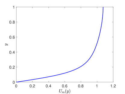
Figure 1: The time mean streamwise flow $U_{m}(y)$ in a turbulent Poiseuille half-channel at $R=1650$.

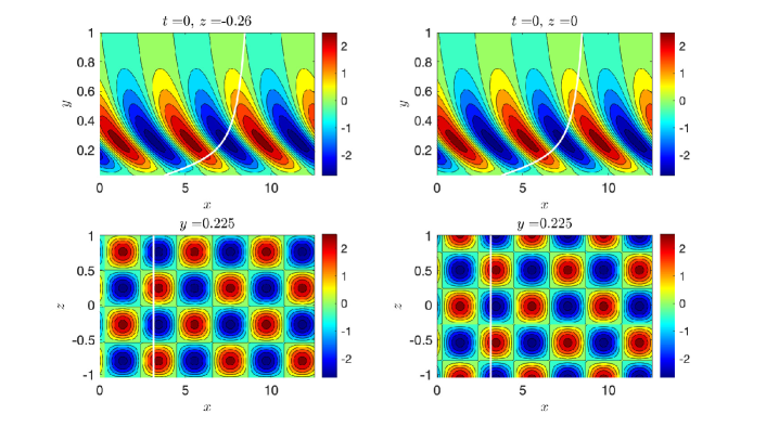
Figure 2: Contours of the cross-stream velocity at initial time of the first sinuous (left panel) and first varicose (right panel) $T=10$ optimal with $k_{x}=3\alpha$. Both of these optimals achieve energy growth $E_{opt}(T)=23.2$. Top panels: contours of cross-stream velocity at $(x,y)$ cross section reveal the expected initial perturbation structure leaning against the shear indicative of growth by the Orr mechanism. The mean flow in Fig. 1 is shown by the white line. Bottom panels: contours of the cross-stream velocity in the $(x,z)$ plane at the specified $y=0.225$. The optimals have identical checker-board sinusoidal structure, with the varicose shifted by a phase of $\pi/2$ in the spanwise direction.

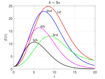
Figure 3: The energy growth as a function of time of the first five pairs of $T=10$ optimals on the mean flow shown in Fig. 1 for perturbations with $k_{x}=3\alpha$ and at $R=1650$. The mean flow has no streak and is exponentially stable.

Up to this point the symmetry axis $z=0$ is arbitrary, but with the emergence of a streak it can be distinguished to be the spanwise location of the streak center. When there is a streak $U_{s}(y,z)$ in the mean flow, which for theoretical convenience will be made symmetric, the sinuous and varicose field components will no longer be spanwise translations of each other and an asymmetry between these two fields develops. Quantities derived exclusively from sinuous perturbations will from now on be indicated with the subscript $s$, while those of varicose form will be indicated with the subscript $v$. We note the following general properties of the Reynolds stresses of sinuous and varicose perturbation fields:

1. When the mean flow has no streak and is spanwise homogeneous the sinuous and varicose perturbation fields specified by (12) and (13) produce equal and opposite force-fields $\bm{f}_{s}=-\bm{f}_{v}$. In this case it is immediate that the Reynolds stresses of the sinuous

   $$\overline{v_{s}w_{s}}=\frac{1}{4}\sin(2k_{z}z)~{}{\rm Re}(\widehat{v}\widehat{w}^{*})~{},~{}~{}\overline{v_{s}^{2}-w_{s}^{2}}=\frac{1}{2}\sin^{2}(k_{z}z)|\widehat{v}|^{2}-\frac{1}{2}\cos^{2}(k_{z}z)|\widehat{w}|^{2}~{}~{},$$ (14)

   and the varicose

   $$\overline{v_{v}w_{v}}=-\frac{1}{4}\sin(2k_{z}z)~{}{\rm Re}(\widehat{v}\widehat{w}^{*})~{},~{}~{}\overline{v_{v}^{2}-w_{v}^{2}}=\frac{1}{2}\cos^{2}(k_{z}z)|\widehat{v}|^{2}-\frac{1}{2}\sin^{2}(k_{z}z)|\widehat{w}|^{2}~{}~{},$$ (15)

   induce equal and opposite torques $G_{x}=\left(\partial_{z}^{2}-\partial_{y}^{2}\right)\overline{vw}+\partial_{yz}\left(\overline{v^{2}}-\overline{w^{2}}\right)$ and therefore equal and opposite force-fields $\bm{f}_{s}=-\bm{f}_{v}$.
   

   

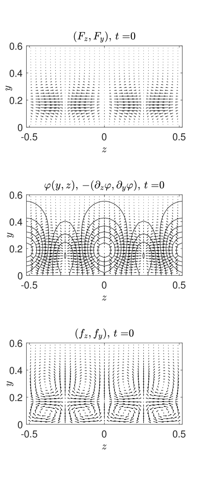
   Figure 4: Top panel: vectors of the total Reynolds stress forcing, $\bm{F}=(F_{z},F_{y})$, given by (3), for the first sinuous optimal in the mean flow shown in Fig. 1. Center panel: contours of the equivalent pressure $\varphi$ of the irrotational part of the Reynolds-stress forcing shown in the top panel. Vectors indicate the force field associated with this pressure field. Bottom panel: vectors of the rotational component of the forcing, $\bm{f}=(f_{z},f_{y})$, that is responsible for inducing the streamwise-mean roll circulation. Shown is the forcing by the $T=10$ sinuous optimal with $k_{x}=3\alpha$ at the initial time. Similar forcing structure characterizes the optimal perturbation at later times.

   

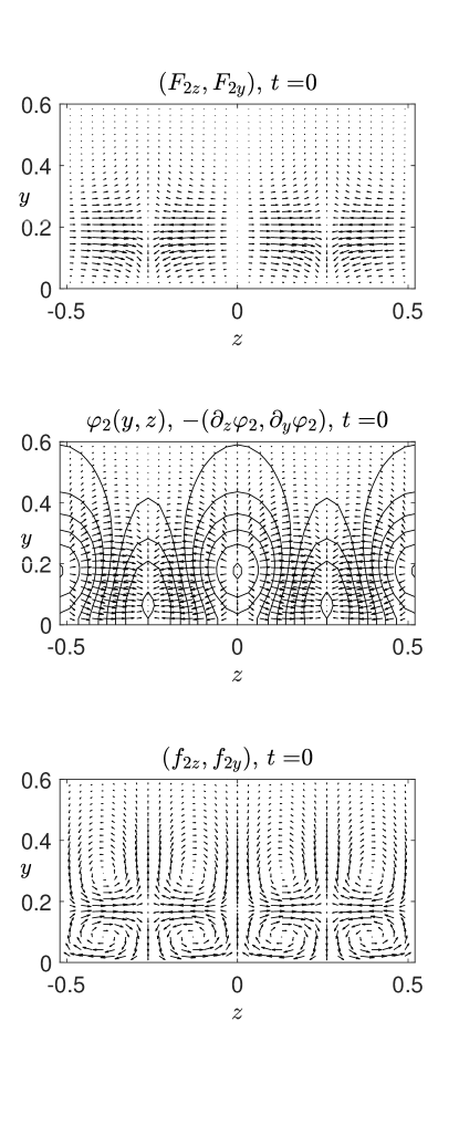
   Figure 5: Top panel: vectors of the dominant Reynolds stress forcing (3), $\bm{F}_{2}=(F_{2z},F_{2y})$, with $F_{2z}=-\partial_{z}w^{2}$ and $F_{2y}=-\partial_{y}v^{2}$ . Center panel: contours of the equivalent pressure $\varphi_{2}$ opposing the irrotational part of the Reynolds-stress forcing of the top panel with arrows showing the force field associated with this pressure field. Bottom panel: vectors with components of the rotational part of the forcing $\bm{f}_{2}=(f_{2z},f_{2y})$ that is primarily responsible for inducing the streamwise-mean roll circulation. For the $T=10$ sinuous optimal with $k_{x}=3\alpha$ at the initial time.

2. In mean flows with a symmetric streak $U_{s}(y,z)$ exclusively sinuous or exclusively varicose perturbations induce rotational force-fields $\bm{f}$, with $y$ components that are symmetric about the symmetry axis of the streak, $z=0$, and $z$ components that are antisymmetric, i.e. $f_{y}(y,z)=f_{y}(y,-z)$ and $f_{z}(y,z)=-f_{z}(y,-z)$. This is a general result arising from the symmetry properties of the velocity fields: under reflection $z\to-z$ exclusively sinuous or varicose fields transform $\overline{vw}$ antisymmetrically and $\overline{v^{2}-w^{2}}$ symmetrically, implying from Eq. (5) that the torque $G_{x}$ transforms antisymmetrically, $G_{x}\to-G_{x}$, and from Eq. (10) that the force field components transform as: $f_{y}\to f_{y}$ , $f_{z}\to-f_{z}$.
   

Comments:

1. The Reynolds stresses of sinuous and varicose perturbations (14) and (15) are anisotropic and produce streamwise-mean torques when $k_{z}\neq 0$, i.e. when two oblique perturbations with $k_{z}\neq 0$ and $k_{x}\neq 0$ interact.

2. Property (a) implies that if a sinuous perturbation in a mean flow $U_{m}(y)$ induces a roll circulation, its companion varicose perturbation induces exactly the opposite roll circulation, and consequently a statistically unbiased and uncorrelated field of perturbations in a spanwise uniform mean flow $U_{m}(y)$ can not induce a streamwise mean roll circulation. However, if spanwise homogeneity is broken by the purposeful introduction of a sinuous or varicose perturbation that breaks the spanwise homogeneity of the perturbation field a roll circulation may be forced. The mechanism of oblique wave interference forcing of roll circulation was proposed by Benney (1960) to be responsible for the emergence of R-S by interfering T-S waves in the experiments of Klebanoff et al. (1962).

3. As discussed, a perturbation field that is spanwise homogeneous can not induce coherent streanwise roll circulations. However, if the streamwise mean flow is infinitesimally perturbed with a streak perturbation $\delta U_{s}$, a homogeneous perturbation field will be distorted so as to break the symmetry of sinuous and varicose components and roll circulations will be induced. Remarkably, at all scales the perturbation field distorted by a streak results in a rotational forcing configured to amplify the distorting streak perturbation. Moreover, the roll forcing is not only correlated to amplify the perturbing streak but also, for perturbationally small streak amplitude, to result in roll forcing proportional to the instigating streak perturbation. i.e. $\delta\Omega_{x}\propto\delta U_{s}$ leading to exponential instability and the emergence of coherent finite amplitude streamwise R-S. This nonlinear instability is a collective instability that has analytic expression only in the equations for the statistics of the Navier-Stokes equations. This instability was analyzed in the framework of a second-order closure of the statistical-state dynamics in Farrell & Ioannou (2012b) and in the full statistical dynamics of the Navier-Stokes equations in Farrell et al. (2017b). This is the instability underlying the formation and maintenance of the R-S in turbulent shear flow that was sought in the linear N-S equations without success because it does not exist in the state component expression of the dynamics.

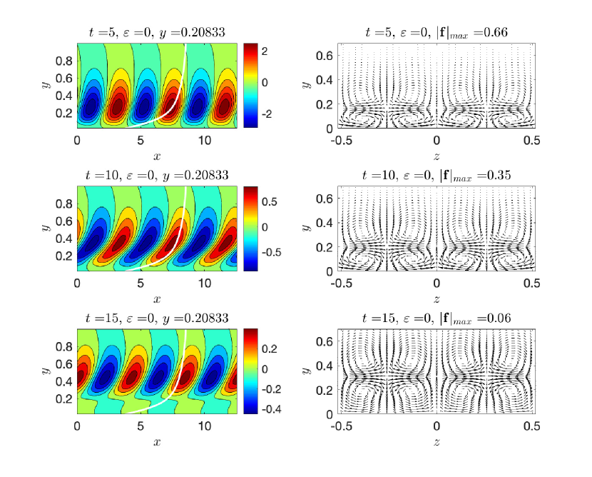
Figure 6: Left panels: Contours in the $(x,y)$ plane of the cross-stream velocity of the first sinuous $T=10$ optimal with $k_{x}=3\alpha$ at times $t=5,10,15$ in the mean flow with no streak. The profile of the mean flow at the cross-section is indicated with the white line. Right panels: Contours of the low-speed streak and vectors at the corresponding times of the Reynolds stress force field that induces the streamwise mean roll circulation in the $(y,z)$ plane. This plot shows that the sinuous optimal at all times induces a roll-circulation that tends through lift-up to form low and high speed streaks. The corresponding varicose perturbation induces the exact opposite circulation. The initial energy of the optimal is $E(0)=0.01$.

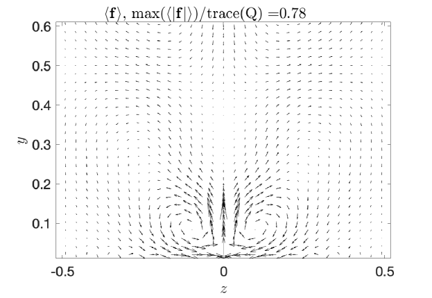
Figure 7: Vectors of the rotational component of the ensemble mean Reynolds stress forcing $\langle\bm{f}\rangle=(\langle f_{z}\rangle,\langle f_{y}\rangle)$ of the streamwise-mean roll circulation for the sinuous components of a stochastically excited perturbation field in the turbulent mean flow shown in Fig. 1 without a streak. The varicose part of the Reynolds stress induces in this case the exact opposite circulation so that for the complete perturbation field the net induced circulation is zero. The plot is for the $k_{x}=3\alpha$ perturbation component.

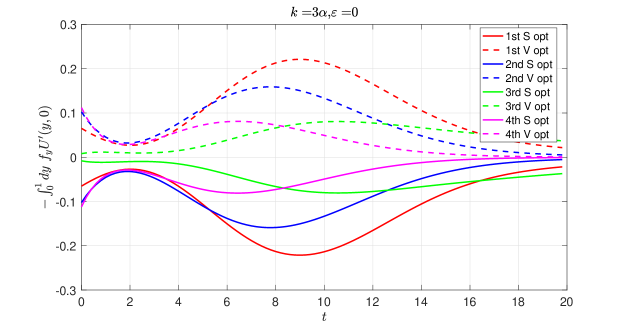
Figure 8: Time evolution of the acceleration of the streamwise-mean streak $-\int_{0}^{1}dy~{}f_{y}U^{\prime}(y,0)$ at $z=0$ by first four $T=10$, $k_{x}=3\alpha$ optimal perturbations. The Reynolds stresses of the sinuous optimals (solid) produce a positive $f_{y}>0$, at the symmetry axis near the wall, and consequently produce roll circulations that tend to form a low-speed streak, while the varicose (dashed) induce equal and opposite roll circulations that tend to form a high speed streak. The induced streamwise acceleration by the optimals is negative at all times for the sinuous perturbations and positive for the varicose. The initial energy of the optimals is $E(0)=0.01$.

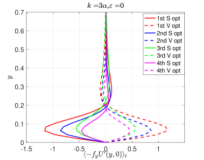
Figure 9: The cross-stream distribution of the time averaged streak acceleration $\langle-f_{y}U^{\prime}(y,0)\rangle_{t}$ at the streak symmetry axis induced by the first four $T=10$ optimals with streamwise wavenumber $k_{x}=3\alpha$. Shown separately are the contributions from perturbations, with sinuous (solid) and varicose (dashed) structure. The initial energy of the optimals is $E(0)=0.01$.

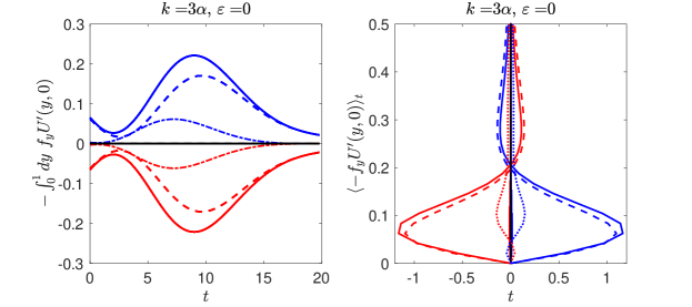
Figure 10: Left panel: Time evolution of the acceleration of the streamwise-mean streak $-\int_{0}^{1}dy~{}f_{y}U^{\prime}(y,0)$ at the symmetry axis $z=0$ induced by the first sinuous (red) and its corresponding varicose (blue) optimal perturbation as shown in Fig. 2. Most of the acceleration is due to the contribution from the $\overline{v^{2}-w^{2}}$ Reynolds stress component (dashed line), the smaller contribution of the $\overline{vw}$ component of the Reynolds stress is indicated with the dotted line. The net acceleration from this pair of optimals (black line) is zero. Right panel: The cross-stream distribution of the time averaged acceleration $\langle-f_{y}U^{\prime}(y,0)\rangle_{t}$. The contribution of $\overline{v^{2}-w^{2}}$ (dashed line) dominates that of the $\overline{vw}$ (dotted line). The initial energy of the optimals is $E(0)=0.01$ and their streamwise wavenumber is $k_{x}=3\alpha$.

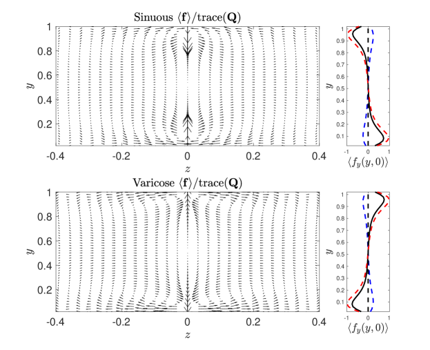
Figure 11: Top panels. Left: vectors of the rotational component of the ensemble mean Reynolds stress forcing $\langle\bm{f}\rangle=(\langle f_{z}\rangle,\langle f_{y}\rangle)$ of the streamwise-mean roll circulation for the sinuous components of a stochastically excited perturbation field with zero mean flow. Right: the cross-stream component $\langle f_{y}(y,0)\rangle$ as function of $y$ at the symmetry axis $z=0$ (black), the dashed-red line is the contribution to $\langle f_{y}(y,0)\rangle$ from the $\overline{v^{2}-w^{2}}$ Reynolds stress, and the dashed blue line is the contribution from the $\overline{vw}$ Reynolds stress. Bottom panels: the corresponding $\langle\bm{f}\rangle$ for the varicose perturbations, which induces the exact opposite circulation so that for the complete perturbation field the net induced circulation is zero. The plot is for the $k_{x}=3\alpha$ perturbation component, which has been stochastically excited with spatially homogeneous forcing in the spanwise. In the cross-stream direction the forcing was weighted by $w=\tanh(y/(5\delta))+\tanh((L_{y}-y)/(5\delta))-1$, where $\delta$ is the cross-stream grid spacing, in order to reduce the forcing adjacent to the boundaries. The forcing amplitudes have been normalized by the energy input by the stochastic excitation.

4 Roll circulation induced by the Reynolds stresses of sinuous and varicose perturbations in a spanwise uniform flow

In the previous section it was shown that the Reynolds stresses of sinuous perturbations in a spanwise uniform mean flow induce roll circulations that are equal and opposite to those induced by their companion varicose perturbations. We demonstrate in this section that sinuous perturbations with symmetry axis $z=0$ induce roll circulations forming low-speed streaks at the symmetry axis, while varicose perturbations induce high-speed streaks.

We choose as mean flow the spanwise-averaged turbulent flow $U_{m}(y)$ obtained from a turbulent channel Poiseuille DNS at $R=1650$ (cf. Fig. 1). Our results have been confirmed to be insensitive to this specific choice. This mean flow was chosen in order to facilitate comparison to DNS data. The $(x,y,z)$ flow domain is ${\cal{D}}\stackrel{{\scriptstyle\mathrm{def}}}{{=}}[0,4\pi]\times[0,1]\times[-\pi/2,\pi/2]$, and the perturbations $\mathbf{u}$ evolve according to (11), and satisfy periodic boundary conditions in $x$ and $z$ and no slip boundary conditions at $y=0,1$. The gravest streamwise wavenumber $k_{x}$ is $\alpha=2\pi/L_{x}$. Our analysis will concentrate on the $k_{x}=3\alpha$ component of the flow because in DNS this component’s Reynolds stresses contributed the most in inducing the streamwise-mean roll circulation. The same qualitative behavior was obtained for the other streamwise components of the flow, indicating that the results discussed exhibit insensitivity to scale.

We consider the Reynolds stresses induced by the optimal perturbations on this mean flow. A $T$-time optimal perturbation is the unit energy initial perturbation, $\mathbf{u}(\mathbf{x},0)$, that leads to the largest energy growth at time $T$, with energy growth:

$$E_{opt}(T)={\rm max}_{\mathbf{u}(\mathbf{x},0)}~{}\left(\frac{\int_{\cal{D}}d^{3}\mathbf{x}~{}|\mathbf{u}(\mathbf{x},T)|^{2}}{\int_{\cal{D}}d^{3}\mathbf{x}~{}|\mathbf{u}(\mathbf{x},0)|^{2}}\right)~{},$$ (16)

(cf. Farrell (1988); Butler & Farrell (1992); Farrell & Ioannou (1996a)). These perturbations provide an optimal orthogonal decomposition of the perturbation field according to their growth over time $T$ in this flow. The optimal perturbations in this mean flow, which is homogeneous both in the streamwise and spanwise direction, are oblique plane waves of the form $\mathbf{u}(y,t)e^{i(k_{x}x+k_{z}z)}$, characterized by their streamwise Fourier wavenumber $k_{x}$ and spanwise wavenumber $k_{z}$. These oblique plane waves can be combined to form symmetric and antisymmetric pairs in the cross-stream $v$ velocity about $z=0$, which is the symmetry axis of the streak that will be introduced in the sequel. In this way the optimals of this spanwise uniform flow can be partitioned into sinuous and varicose perturbations with structure given by Eqs. (12) and (13). The structure of the cross-stream velocity of the first pair of sinuous and varicose $T=10$ optimals with $k_{x}=3\alpha$ are shown in Fig. 2. Because of the spanwise translation symmetry of the mean flow each $(k_{x},k_{z})$ pair of optimals with the same cross-stream structure will have identical energy evolution. For example, the energy growth of the first five $k_{x}=3\alpha$ pairs of sinuous and varicose $T=10$ optimal perturbations are shown in Fig. 3.

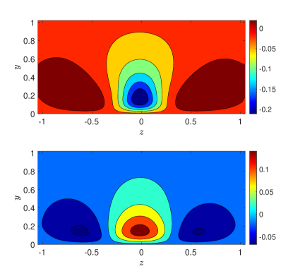
Figure 12: Contours of the velocity of the equilibrium low-speed streak (upper panel) and high-speed streak (lower panel) in turbulent Poiseuille flow at $R=1650$ in a channel with $L_{x}=4\pi$ and $L_{z}=\pi$. The spacing of the contours is $0.04$.

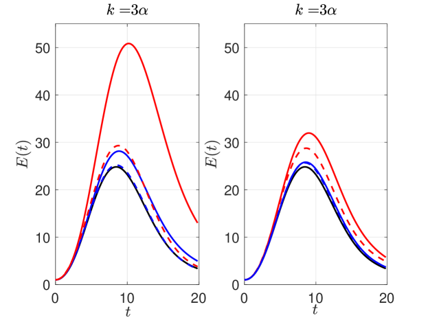
Figure 13: Time evolution of the energy of the first (solid lines) and second (dashed lines) $T=10$ optimals in a flow with a low speed streak (left panel) and a high-speed streak with the same structure (right panel) for streak amplitude $\varepsilon=0.4$ and $\varepsilon=1$. The energy growth of the optimals in the mean flow with $\varepsilon=\pm 1$ are indicated with red, those with $\varepsilon=\pm 0.4$ with blue, and those with no streak $\varepsilon=0$ with black. The first optimal has sinuous structure while the second has varicose structure. This figure shows that the spanwise shear increases the energy growth of both perturbations but that the low-speed streak supports substantially greater optimal growth compared to that supported by the high speed streak. Perturbations have $k_{x}=3\alpha$.

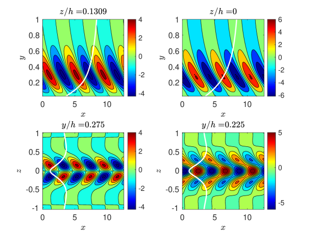
Figure 14: Contours of the cross-stream velocity of the first sinuous (left panel) and first varicose (right panel) $T=10$ optimal for $k_{x}=3\alpha$ at the initial time with mean flow $U(y,z)=U_{m}(y)+U_{s}(y,z)$ in which $U_{m}(y)$ is the spanwise averaged turbulent mean flow shown in Fig. 1 and $U_{s}$ is the equilibrium low-speed streak shown in Fig. 12 (upper panel). The presence of the streak centers and confines the optimals at the streak minimum and breaks the symmetry between the sinuous and varicose pairs. The sinuous achieves the highest energy growth of $50$ at $t=10.4$, while the varicose reaches energy growth $29$ at $t=8.8$. Top panels: contours of cross-stream velocity in an $(x,y)$ cross section show the typical initial configuration of an optimal perturbation which is that it leans against the shear as expected for growth by the Orr mechanism. The profile of the mean flow is shown by the solid white line. Bottom panels: contours of the cross-stream velocity in the $(x,z)$ plane at $y=0.275$. The optimals are obliques waves configured to transfer mean flow energy from the spanwise shear to the perturbation. The profile of the mean flow is the solid white line. The flow is at $R=1650$ in a doubly periodic channel with $L_{x}=4\pi$, $L_{z}=2$, and $\alpha=2\pi/L_{x}$.

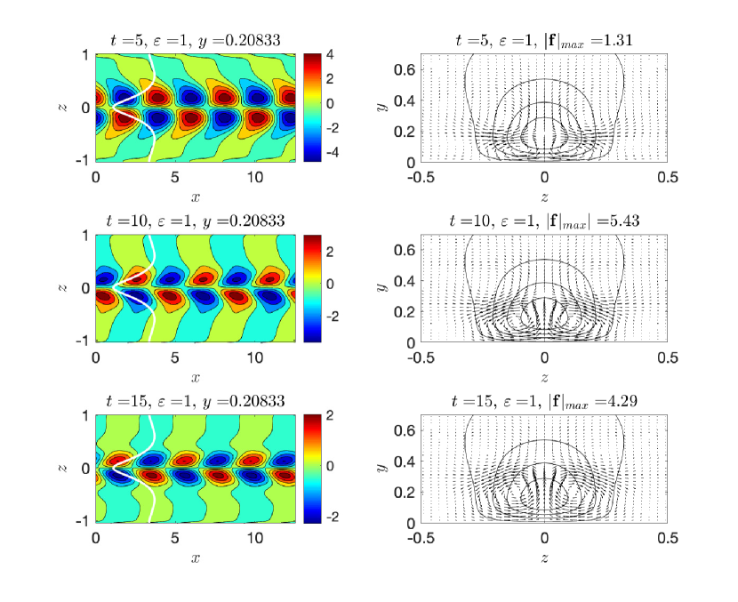
Figure 15: Left panels: Contours in the $(x,z)$ plane of the cross-stream velocity of the first sinuous $T=10$ optimal with $k_{x}=3\alpha$ at times $t=5,10,15$ in the mean flow with the equilibrium low-speed streak. The profile of the streak at the cross-section is indicated with the white line. Right panels: Contours of the low-speed streak and vectors at the corresponding times of the Reynolds stress force field that induces the streamwise mean roll circulation in the $(y,z)$ plane. The maximum magnitude of the force occurs here at the symmetry axis of the streak. This plot shows that the sinuous optimal at all times induces a roll-circulation that tends through lift-up to amplify the low-speed streak. The initial energy of the optimal is $E(0)=0.01$.

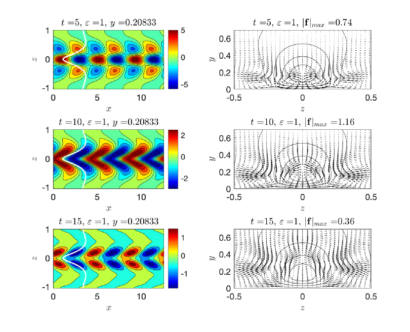
Figure 16: As in Fig. 15 for the first varicose optimal. This plot shows that the varicose optimal at all times induces a roll-circulation that tends through lift-up to destroy the low-speed streak. However the varicose mode induces a weaker circulation than the sinuous and the net circulation from the first sinuous and varicose optimals results in amplification of the streak as shown in Fig. 17. The maximum magnitude of the force does not occur at the symmetry axis of the streak.The initial energy of the optimal is $E(0)=0.01$.

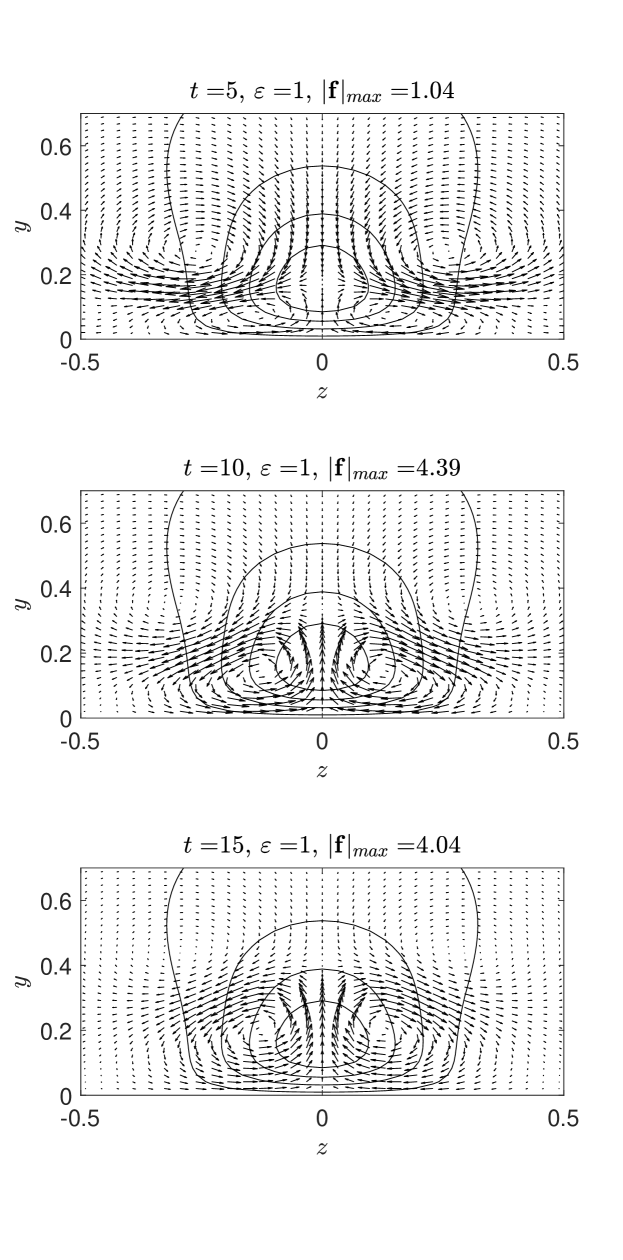
Figure 17: As in Fig. 15 but vectors of the total force $\mathbf{f}=(f_{y},f_{z})$ obtained by adding the force by the first sinuous optimal to the force by the first varicose optimal. The initial energy of the optimals is $E(0)=0.01$.

Figure 18: As Fig. 14 but for the first sinuous and varicose $T=10$ optimals for the mean flow $U(y,z)=[U]_{z}-U_{s}(y,z)$, with high-speed streak the mirror image of the low-speed streak of Fig. 12. The first optimal is still sinuous achieving energy growth $32$ at $t=8.4$ while the second optimal is varicose and it evolves almost identically with the sinuous achieving maximum energy growth $29$ at $t=8.6$. Note that sinuous and the varicose first optimals have almost the same oblique wave structure and that both perturbations are located at the wings of the streak.

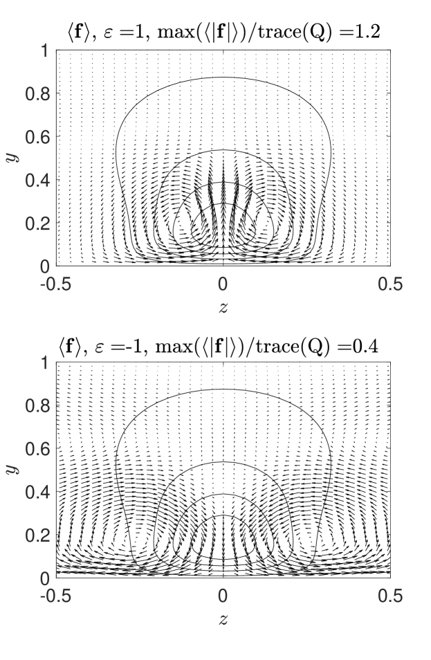
Figure 19: Contours of the equilibrium low-speed streak and vectors of the ensemble mean force field, $\langle\mathbf{f}\rangle$, when the $k_{x}=3\alpha$ perturbation field is stochastically excited white in energy in a mean flow with the low-speed with $\varepsilon=1$ (upper panel) and with the high-speed streak with $\varepsilon=-1$ (lower panel). The response is normalized by the energy introduced in the flow, ${\rm trace}(\bm{\mathsf{Q}})$, where $\bm{\mathsf{Q}}$ is the forcing covariance in energy coordinates.

To understand the streamwise-mean roll circulation induced by these optimal perturbations we first plot the divergent total force-field $\bm{F}=(F_{y},F_{z})$ produced by the Reynolds stresses of the sinuous optimal perturbation at the initial time in Fig. 4 (top panel) and perform a Helmholtz-Hodge decomposition of this force-field in order to determine the characteristics of the residual field $\bm{f}$ that determines the forcing of the roll circulation. The total force field $\bm{F}$ with components $F_{y}=-\partial_{z}\overline{vw}-\partial_{y}\overline{v^{2}}$ and $F_{z}=-\partial_{y}\overline{vw}-\partial_{z}\overline{w^{2}}$ is strongly divergent at the symmetry axis $z=0$ and is almost completely aligned in the spanwise direction, $\hat{\mathbf{z}}$, i.e. $\bm{F}\approx-\partial_{z}\overline{w^{2}}~{}\hat{\mathbf{z}}$. For sinuous perturbations $-\overline{w^{2}}$ has a minimum at $z=0$ and therefore the induced $\bm{F}$ is divergent in the region about $z=0$, as is evident in Fig. 4 (top panel). The opposite situation occurs for varicose perturbations. The divergent component of $\bm{F}$ is opposed by the pressure field, $\varphi$, that develops. Contours of the pressure, $\varphi$, and the resulting force field opposing the divergent component of the Reynolds stress force, $-\bm{\nabla}\varphi$, are shown in Fig. 4 (center panel). The force from the pressure field is isotropic, and given that $\bm{F}$ is divergent along $z=0$, the pressure force will be directed towards the channel boundary near the wall and away far from the wall. This implies that as $\bm{F}$ has a very small component in the cross-stream direction the residual $\bm{f}$ will have a strong positive cross-stream component $f_{y}>0$ at the symmetry axis. Further from the wall the residual force direction reverses, and the overall force field $\bm{f}$ has quadrupole structure at the symmetry axis, as seen in Fig. 4 (lower panel).

Crucial to the above argument is the dominance of the force field induced by the $\overline{v^{2}-w^{2}}$ components of the Reynolds stress over the contribution of the $\overline{vw}$ Reynolds stress. This is shown in Fig. 5 where the Helmholtz-Hodge decomposition of the force field induced by this Reynolds stress with components $\bm{F}_{2}=(F_{2y},F_{2z})=(-\partial_{y}\overline{v^{2}},-\partial_{z}\overline{w^{2}})$ can be compared to the decomposition of the full force field field $\bm{F}$ in Fig. 4. The dominance of the $\overline{v^{2}-w^{2}}$ Reynolds stress is maintained during the whole evolution of the optimal and is the reason, as we will see, underlying the direction of the induced roll-circulation of the sinuous and the varicose perturbations. It should be noted that the smaller contribution from the $\overline{vw}$ Reynolds stress changes structure and sign during the evolution. We find that dominance of the $\overline{v^{2}-w^{2}}$ Reynolds stress also characterizes the DNS statistics.

The force field structure of $\bm{f}$ persists throughout the evolution of the optimal, as shown in Fig. 6, and each developing optimal forces a coherent roll circulation that through lift-up forms a low-speed streak near the wall at the symmetry axis. This particular circulation structure results from the sinuous form of the perturbations and is not limited to the first sinuous optimal. We demonstrate that by calculating the ensemble mean force $\langle\bm{f}\rangle$ that arises when all the sinuous components of the flow are equally excited stochastically. The ensemble mean statistics are calculated by determining the ensemble mean spatial covariance $\bm{\mathsf{C}}$ of the velocity components which satisfies at statistical equilibrium the Lyapunov equation

$$\bm{\mathsf{A}}\bm{\mathsf{C}}+\bm{\mathsf{C}}\bm{\mathsf{A}}^{\dagger}=-\bm{\mathsf{Q}}~{},$$ (17)

where $\bm{\mathsf{A}}$ is the linear operator governing the perturbation dynamics in Eq. (11), and $\bm{\mathsf{Q}}$ is the spatial covariance of the delta-correlated stochastic forcing, chosen here to be the identity in energy coordinates so that equal energy input is imparted to all degrees of freedom (cf. Farrell & Ioannou (1993d, 1996a)). The stability of $\bm{\mathsf{A}}$ ensures that the statistical steady state exists. From the covariance the ensemble mean Reynolds stresses can be obtained and from them the ensemble mean roll forcing and the lift-up induced streamwise acceleration cf. Farrell & Ioannou (2012a).

The ensemble mean force $\langle\bm{f}\rangle$ from the sinuous components of the stochastically excited flow is shown in Fig. 7. This is the force field averaged over time if all sinuous optimals are excited and their Reynolds stress contribution superposed. Fig. 7 shows that the ensemble mean Reynolds-stress force-field from the sinuous perturbations induces roll circulations that tend to form a low-speed streak near the wall at the symmetry axis. Varicose perturbations induce the exact opposite roll-circulations and is not shown. The resulting roll circulation at the center $z=0$ is similar to the roll circulation induced by the first sinuous optimal. However the stochastically excited flow results in a roll circulation that is concentrated at the symmetry axis and has smaller spanwise wavenumber. This is caused by cancellations of the induced circulations that occur far from the symmetry axis as the roll circulations from the various sinuous optimals add constructively at the symmetry axis and destructively away from it. This phenomenon of localization of the roll circulation is observed during transition to turbulence. Generically, streaks emerge during transition as an exponential instability of the interaction of the mean flow and the perturbation field in the background of free-stream turbulence, an instability that has analytical expression in the framework of second order closure of the statistical dynamics of the channel flow (S3T) (Farrell & Ioannou, 2012b; Farrell et al., 2017b). The streaks that initially emerge are almost sinusoidal and inherit the spanwise wavenumber of the most unstable mode arising in the S3T closure equations. But as transition proceeds and the streaks grow the spanwise length-scale increases dramatically as a broad spectrum perturbation field starts being sustained with its Reynolds stresses contributing to localizing the roll circulation.

To quantify the development over time of the rotational force $\bm{f}$ generating streaks by lift-up, the time development of quantity $-f_{y}U^{\prime}(y,0)$ at the streak symmetry axis (with $U^{\prime}(y,0)\stackrel{{\scriptstyle\mathrm{def}}}{{=}}\partial_{y}U$ at the symmetry axis) is shown in Fig. 8 and Fig. 9. This quantity measures the lift-up induced acceleration of the streamwise mean velocity at the symmetry axis. Fig. 8 shows the time evolution of the net induced streamwise-mean streak $-\int_{0}^{1}dy~{}f_{y}U^{\prime}(y,0)$ at the symmetry axis by the first four pairs of sinuous and varicose optimals. The figure shows that at all times the sinuous optimals induce a low speed streak, while the corresponding varicose optimals induce an equal high-speed streak. The time averaged cross-stream distribution of the induced streak acceleration $\langle-f_{y}U^{\prime}(y,0)\rangle_{t}$ at the symmetry axis by the evolving first four pairs of sinuous and varicose optimals is shown in Fig. 9. That the contribution of the Reynolds stress component $\overline{v^{2}-w^{2}}$ dominates that of $\overline{vw}$ during the development of the first pair of sinuous and varicose optimals is shown in Fig. 10.

We have seen that key property of the sinuous and varicose perturbations to determining the direction of their induced roll forcing is the dominance of the $F_{z}=-\partial_{y}\overline{vw}-\partial_{z}\overline{w^{2}}$ Reynolds stress force component over the $F_{y}=-\partial_{z}\overline{vw}-\partial_{y}\overline{v^{2}}$ component. Dominance of $F_{z}$ is due to dominance of the $\overline{w^{2}}$ over $\overline{v^{2}}$, which in turn is due to the $\overline{v^{2}}$ fluctuations being preferentially suppressed compared to the $\overline{w^{2}}$ by the solid boundary condition at the wall. This asymmetry between $\overline{w^{2}}$ and $\overline{v^{2}}$ near a boundary is a property connected to the presence of the wall and is not fundamentally dependent on the presence of wall-normal shear or the presence of a particular type of perturbation, such as an optimally growing perturbation, other than its being sinuous or varicose. We demonstrate this by showing that stochastically excited sinuous perturbations in a channel with zero mean flow produce a roll-inducing Reynolds stress force field. This resulting roll-inducing force field, shown in Fig. 11, has the characteristic quadrupole structure and is concentrated near the walls as is the case for optimal perturbations of sinuous and varicose form. When the mean flow has wall-normal shear the roll-inducing force field is concentrated in the shear region, as shown in Fig. 7, and in this case it is the energy bearing optimal perturbations, and their $\overline{v^{2}}$ field decaying faster than their $\overline{w^{2}}$ field near the wall, that dominate the perturbation field and are responsible for the structure of the resulting Reynolds stress roll-forcing.

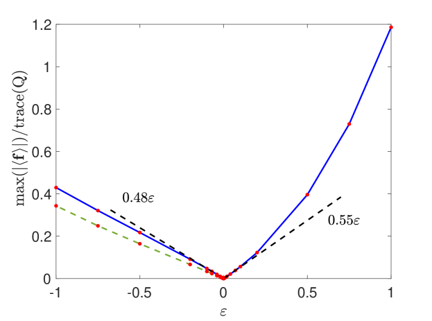
Figure 20: The magnitude of the maximum ensemble mean force $\mathbf{f}=(f_{y},f_{z})$ produced by the Reynolds stresses as a function of the amplitude of the streak $\varepsilon$. This maximum occurs at the symmetry axis of the streak. The roll-circulation induced is in a direction to accelerate both the low-speed, $\varepsilon>0$, and the high-speed streaks, $\varepsilon<0$. The dashed green line is the force induced when the high-speed streak has the structure of the equilibrium high-speed streak shown in Fig. 12 (lower panel). The $k_{x}=3\alpha$ perturbations are stochastically excited by a stochastic excitation that injects ${\rm trace}(Q)$ units of energy density per unit time.

5 Roll circulation induced by the Reynolds stresses of sinuous and varicose perturbations in the presence of a streak

We have demonstrated that oblique waves, individual optimal perturbations, sums of optimal perturbations and general stochastically forced perturbations with sinuous form force roll circulations as do oblique waves, optimals, sums of optimals and general perturbations with varicose form. However, the tendency of sinuous perturbations to form rolls configured to force low speed streaks is exactly canceled in a spanwise statistically homogeneous flow by the tendency of varicose optimals to form rolls with opposite sign configured to force high speed streaks. It remains to show how the imposition of a perturbation streak breaks the cancellation of tendencies in forcing between the sinuous and varicose components resulting in the instability that is responsible for the formation and maintenance of the R-S in shear flow.

In this section we discuss the Reynolds stresses induced by perturbations in mean flows with a streak of the form $U=U_{m}(y)+\varepsilon U_{s}(y,z)$, with $\varepsilon$ a parameter modulating the amplitude and sign of the streak. The streamwise mean flow $U_{m}(y)$ is the half-channel time mean flow in Poiseuille turbulence at $R=1650$, shown in Fig. 1, and $U_{s}(y,z)$ is the equilibrium low-speed streak shown in Fig. 12 (upper-panel) which is obtained by time averaging the low-speed streaks of the turbulent flow. With this choice of $U_{s}$, when $\varepsilon>0$ low-speed streaks are introduced in the flow with the shape of the low-speed streak, and when $\varepsilon<0$ high-speed streaks are introduced that are mirror images of the corresponding low-speed streaks. We choose this family of high-speed streaks, instead of those that arise from the equilibrium high-speed streak (cf. lower panel of Fig. 12) in order to reduce the number of parameters. Comparisons were made with high-speed streaks in the shape of the equilibrated high-speed streak of Fig. 12. The results presented here were found to be robust and not sensitive to this detail.

Upon introduction of a spanwise symmetric streak the perturbations were found to localize about the center of the streak. The sinuous and varicose perturbations continue to induce roll circulations predominantly from the Reynolds stress associated with $\overline{v^{2}-w^{2}}$, as previously described, and as previously described these roll circulations induce respectively low and high-speed streak perturbations. However, the introduction of the streak creates a crucial difference which is an imbalance between the sinuous and varicose perturbations. With no streak the net circulation induced by corresponding sinuous and varicose perturbations cancel. In the presence of a low-speed streak the sinuous perturbations are favored over the varicose and the induced net roll circulation tends to reinforce the low-speed streak, while in the presence of a high-speed streak the varicose perturbations are favored resulting in a net roll circulation that tends to reinforce the high-speed so that in both cases the Reynolds-stress induced circulation reinforces the pre-existing streak. We will demonstrate this dynamics for the first pair of optimal perturbations in the flow and for the ensemble response when a flow with a streak is stochastically excited by temporally and spatially uncorrelated forcing.

We choose $k_{x}=3\alpha$ perturbations. This choice of streamwise wavenumber was made because it is the wavenumber that induces the strongest roll circulation both in DNS and when the flow with the equilibrium low-speed streak is stochastically excited. This choice of streamwise wavenumber for the optimal does not change qualitatively the results that are presented. The energy growth of the first pair of $T=10$ sinuous and varicose optimals is shown in Fig. 13 for low-speed streaks (left panel) and their mirror high-speed streaks (right panel) with with streak amplitude $\varepsilon=0,\pm 0.4,\pm 1$. This figure shows that the optimal perturbation growth increases as the amplitude of the streak increases and that the increase is substantial when the streak is low-speed and marginal when the streak is high-speed. Energy transfer from the mean spanwise shear to the perturbations, $-\int_{\cal D}dydz~{}\overline{uw}U_{z}$, is the energy source that accounts for the increased perturbation growth in the presence of the streak, and especially so when a low-speed streak is present because flows with low-speed streaks have a relatively smaller wall-normal shear and the perturbations are less readily sheared over by the wall-normal shear, which limits their potential growth.

Differences in the growth of perturbations in flows of the form $U_{m}(y)\pm\varepsilon U_{s}(y,z)$ is expected, because the flows are not mirror images of each other. But such pronounced asymmetry in the growth of optimal perturbations in low-speed and their mirror high-speed streaks is surprising and has dynamical implications. It implies, as we will show, that high-speed streaks are supported weakly by their Reynolds stresses, which provides an explanation for the dominance of low-speed streaks in wall-bounded turbulence. Fig. 13 also shows that in low-speed streak flows the sinuous optimal perturbations achieve substantially greater energy growth than their companion varicose perturbations. The structure of the top pair of optimals is shown in Fig. 14. As $\varepsilon$ increases the perturbations become increasingly localized at the center of the low-speed steak. Note that the sinuous perturbations are concentrated at the wings of the streak, where there is larger spanwise mean shear. This is consistent with the observation that sinuous perturbations grow more than the corresponding varicose perturbation, which are concentrated at the center of the streak where the shear is small.

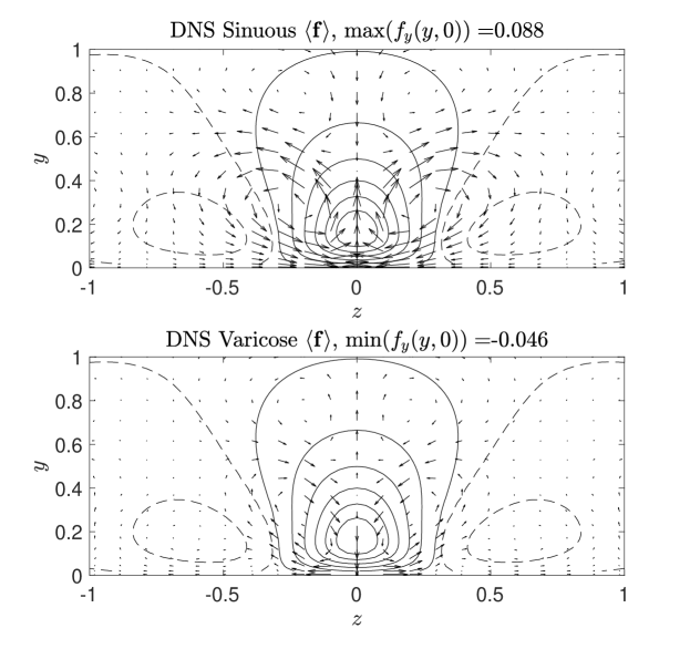
Figure 21: Contours of the low-speed streak (solid: negative values, dashed: positive values) and vectors of the force field, $\langle\mathbf{f}\rangle$, induced by the time mean Reynolds stresses in the DNS low-speed streak. Upper panel: the force field induced by the sinuous components of the flow. In agreement with the discussion, they tend to support the low-speed streak. Lower panel: the force field induced by the varicose components of the flow, which tends to destroy the low-speed streak. The force field of the total perturbation field is shown in Fig. 22 (upper-panel).

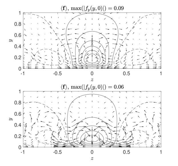
Figure 22: Vectors of the force field, $\langle\mathbf{f}\rangle$ induced by the time mean Reynolds stresses in the DNS low-speed streak (upper panel) and the high-speed streak (lower panel). The contours show the respective profile of the average low and high speed streaks in the DNS Top panel: solid line contours for negative values, dashed for positive values. Bottom panel: solid line contour for positive values, dashed for positive values. The contour level is 0.03, cf. Fig. 12.

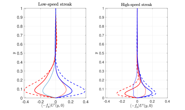
Figure 23: The cross-stream distribution of the net mean acceleration $-f_{y}U^{\prime}(y,0)$ from the sinuous (red lines) and varicose (blue lines) $k_{x}=3\alpha$ perturbations in the time-averaged low-speed streak (left panel) and in the time averaged high-speed streak (right panel). The streaks are shown in Fig. 12. The dashed lines shows the contribution to the induced acceleration from the Reynolds stress $\overline{v^{2}-w^{2}}$ and the dotted lines the contribution from the $\overline{vw}$ Reynolds stress. The net Reynolds stress acceleration from the total perturbation field tends to support both the low-speed streak and the high-speed streak. Data from a DNS simulation.

The time development of the sinuous optimal structure and plots of the resulting rotational Reynolds stress force field $\bm{f}$ are shown in Fig. 15. This figure shows that the sinuous optimal induces a coherent roll-circulation that tends to reinforce the low-speed streak. The reverse roll circulation is induced by the companion varicose optimal, shown in Fig. 16. However, in the presence of the low-speed streak the streak opposing circulation of the varicose perturbation is weaker than the streak amplifying circulation of the sinuous optimal. Hence, in the presence of even the slightest streak, the net circulation from the top pair of optimals tends to reinforce the low-speed streak, as indicated in Fig. 17. The reverse situation occurs in the high-speed streak. In that case although at $\varepsilon=-1$ the sinuous optimal grows slightly more than the varicose, the Reynolds stresses from the varicose dominate and the net circulation tends to reinforce the high-speed streak. The optimals in this case have very similar structure (cf. Fig. 18) and nearly identical evolution and the net circulation induced from the superposition of the opposing and almost identical sinuous and varicose components is weak compared with the circulation induced by the optimals in the low-speed streak flow.

We confirm the robustness of our conclusions about the roll forcing pattern that was obtained by analysis of the top pair of optimals by considering the general case of roll forcing by the ensemble mean Reynolds stresses of the perturbation field resulting when all degrees of freedom are excited stochastically and equal in energy. The ensemble mean force field $\bm{f}$ induced when there is a low-speed streak present in the flow is shown in Fig. 19 (upper-panel), showing that in low-speed streak flows the sinuous perturbation component dominates the statistics. In a high-speed streak flow, Fig. 19 (lower-panel), the induced roll circulation reverses with the varicose modes dominating the statistics. Note that the induced force is stronger when there is a low-speed streak. The dependence of the amplitude of the induced force-field on the amplitude of the streak is plotted in Fig. 20 from which it is apparent that a low-speed streak is more vigorously supported by the Reynolds - stresses and this remains true when the calculation is repeated using the high-speed streak with the structure of the equilibrium high-speed streak that that is obtained in DNS (cf. lower panel of Fig. 12). The direction of the induced force, which always tends to increase the pre-existing streak, and the linear dependence of the induced force on streak amplitude, when the the amplitude of the streak is small, indicates that the interaction between streaks and perturbations is consistent with the necessary requirement for producing an exponential instability. This instability has been analytically studied using the S3T form of statistical state dynamics (Farrell & Ioannou, 2012a; Farrell et al., 2017b).

6 Comparison with DNS data

Abbreviation	$[L_{x},L_{y},L_{z}]$	$[L^{+}_{x},L^{+}_{y},L^{+}_{z}]$	$N_{x}\times N_{z}\times N_{y}$	$R_{\tau}$	$R$
NL100	$[4\pi\;,\;2\;,\;\pi]$	[1264 , 201 ,316]	$128\times 63\times 97$	$100.59$	1650

Table 1: The simulation of the plane parallel Poiseuille flow was performed in a channel of streamwise, wall-normal and spanwise length $[L_{x},L_{y},L_{z}]$, with periodic boundary conditions in $x$ and $z$ and no slip boundary conditions at the channel walls $y=0$ and $y=2$. Lengths have been made nondimensional by $h$ the channel half-width, velocities by $\langle U\rangle_{c}$, the center velocity of the time-mean flow, and time by $h/\langle U\rangle_{c}$. The Reynolds number is $R=\langle U\rangle_{c}h/\nu$, with $\nu$ the kinematic viscosity. $[L^{+}_{x},L^{+}_{y},L^{+}_{z}]$, indicate the domain size in wall-units. $N_{x}$, $N_{z}$ are the number of Fourier components after dealiasing and $N_{y}$ is the number of Chebyshev components. $R_{\tau}=u_{\tau}h/\nu$ is the Reynolds number of the simulation based on the friction velocity $u_{\tau}=\sqrt{\nu\left.\textrm{d}\langle U\rangle/\textrm{d}y\right|_{\rm w}}$,where $\left.\textrm{d}\langle U\rangle/\textrm{d}y\right|_{\rm w}$ is the shear at the wall.

Observational support for the theoretical arguments that we have presented was obtained in the DNS data of Poiseuille flow at $R=1650$. Details of the simulation are given in Table 1. From the DNS we have obtained the average low-speed streak and average high-speed streak, shown in Fig. 12, along with their associated perturbation field statistics. The streaks, which were nearly symmetric in the spanwise direction, were symmetrized and the average Reynolds stresses of the sinuous and varicose components of the perturbation field were obtained. We present here the roll-circulation induced by the $k_{x}=3\alpha$ component of the perturbation field that produces the largest streamwise-mean torque in DNS.

The roll-inducing force field $\bm{f}$ produced by the sinuous component of the perturbation field of the low-speed streak is shown in Fig. 21 (upper panel) and that produced by the varicose component in Fig. 21 (bottom panel). The sinuous component of the DNS tends to amplify the low-speed streak, while the varicose tends to induce a weaker reverse circulation, in agreement with the theoretical discussion in the earlier sections. In Fig. 22 (top panel) the roll-inducing component of the force field, $\bm{f}$, produced by the entire perturbation field is shown, which, as discussed above, supports the low-speed streak. It was confirmed that the rotational force $\bm{f}$ of the total perturbation field is very close to the sum of the rotational forcing by the sinuous and varicose components. This indicates that there is no substantial correlation between the sinuous and varicose components of the flow giving rise to cross-term contributions to the Reynolds stresses, so that the total rotational force $\bm{f}$ and that obtained from the analysis performed in this paper, in which the sinuous and varicose components independently add, is justified. In Fig. 22 (bottom panel) is shown the roll-inducing force field $\bm{f}$ of the total perturbation field in the high-speed streak, which as expected supports the high-speed streak, while the support is weaker than that of the $\bm{f}$ in the low-speed streak, as in our previous discussion.

In Fig. 23 we plot the contribution of the $\overline{v^{2}-w^{2}}$ and $\overline{vw}$ Reynolds stresses to the cross-stream acceleration of the sinuous and varicose components of the perturbation field in the mean low-speed streak (left panel) and the mean high-speed streak (right panel). As expected dominant contribution to $\bm{f}$ is confirmed to be due to $\overline{v^{2}-w^{2}}$.

7 Discussion

The study of turbulence dynamics has roots in interpretation of spatial and temporal spectra (Taylor, 1935, 1938; Kolmogorov, 1941). At the time, data were available from two point space or time correlations which allowed spectra to be determined. Unfortunately this required the phase of Fourier components to be left indeterminant and so implicitly the maximum entropy assumption of random phase was made. The result was that turbulence theory neglected the role of coherent structures the study of which requires determining the phase of Fourier components. The origin of structures elicited by the observational techniques available was commonly ascribed to modal instability based on Rayleigh’s theory of modes (Rayleigh, 1880, 1896). However, smoke and hydrogen bubbles tended to reveal three dimensional structures that did not correspond with modes of maximal growth rate and in fact the canonical laboratory shear flows did not support growing modes. The first 3D turbulence to be comprehensively observed was that of the baroclinic turbulence of the midlatitude atmosphere. This was accomplished soon after the invention of the vacuum tube which allowed telemetry from weather ballooons to be made over the entire troposphere. Twice daily radiosonde observations covering the entire Northern Hemisphere soon followed. The primary coherent structures revealed by this comprehensive data set was the midlatitude cyclone and the jet stream. The midlatitude cyclone was quickly identified with an unstable mode of the equations of motion linearized about the mean jet flow (Charney, 1947; Eady, 1949) while the coherent jet stream structure was determined to result from the cooperative interaction between the midlatitude cyclones and the jet, the requisite upgradient momentum flux required for the cyclone perturbations to maintain the jet being ascribed to “negative viscosity” (Jeffreys, 1933; Starr, 1953, 1968). It is remarkable that the two primary mechanisms of coherent structure formation in turbulence, selective perturbation growth in the linearized equations of motion and cooperative nonlinear interaction between essentially stochastic turbulent perturbations and the coherent structure had already been recognized within a decade after comprehensive observations of a turbulent flow became available. While the fundamental energy source for maintaining the coherent structure by these two dynamical mechanisms had been identified, the predictions of the analysis of these mechanisms was soon shown to be at variance with observation: the growth of cyclones did not correspond with the growth of modes and the satisfaction of necessary conditions for instability did not allow prediction of cyclone formation. In the case of the second mechanism, while negative viscosity provided a suggestive analogy for the upgradient eddy momentum fluxes giving rise to the polar jet; as a parameterization in the equations of motion it did not result in an analytic theory that predicted jet stream formation in agreement with observations. Lack of agreement of observed cyclogenesis with modal theory was subsequently explained by identification of cyclone formation with non-normal transient growth of stable optimally growing perturbations arising in the turbulence (Farrell, 1982, 1984, 1985, 1989a, 1989b) in which case the dynamics is properly analyzed using generalized stability theory (GST) (Farrell & Ioannou, 1996a, b). Understanding the mechanism of jet stream formation has roots in the identification of equilibrium structures in stochastic turbulence models (DelSole & Farrell, 1996) and obtained full analytic development with the advent of statistical state dynamics methods (Farrell & Ioannou, 2003, 2007; Srinivasan & Young, 2012; Parker & Krommes, 2013, 2014; Constantinou et al., 2016; Farrell et al., 2017a; Farrell & Ioannou, 2019). In wall-bounded shear flow turbulence theory the non-normal transient growth mechanism for analyzing coherent structure formation was introduced in the case of 2D structures in Farrell (1988) and in the case of 3D structures in Butler & Farrell (1992, 1993); Farrell & Ioannou (1993a, b); Reddy & Henningson (1993); Trefethen et al. (1993); Schmid & Henningson (2001). Formation of the R-S by a cooperative instability mechanism was advanced by Hamilton et al. (1995); Waleffe (1997) and the operative mechanism was identified in Farrell & Ioannou (2012a); Farrell et al. (2017b). More recently methods based on GST have been advanced ascribing the R-S to the growth of individual optimals (Jiménez, 2013, 2018) and alternatively to the excitation of the zero frequency resolvent (McKeon & Sharma, 2010; McKeon, 2017). However, in the case of 3D wall-bounded shear flow it has not been determined whether and in which cases the non-normal transient growth mechanism explains an observed R-S and in which cases the observation is explained by the cooperative instability mechanism, that is whether SSD analysis rather than non-normal transient growth analysis using GST is appropriate.

8 Conclusions

Our analysis reveals the remarkable universal tendency of sinuous perturbations in channel flows to induce through their Reynolds stresses roll circulations and also for varicose perturbations to induce roll circulations of opposite sign. This happens even in a stochastically forced channel with no mean flow. We have ascribed this result to the presence of solid wall boundaries which constrain the flow so that the wall normal velocity fluctuations decay to zero faster than the spanwise velocity fluctuations. However, when the mean flow has no spanwise variation the sinuous and varicose perturbations induce roll circulations that cancel each other. Furthermore, we have shown that even a streak at perturbative amplitude can organize turbulent perturbation Reynolds stresses so as to amplify the perturbing streak which destabilizes the R-S in turbulent shear flows. The reason for this universal streak amplification property is revealed by the partitioning of the turbulent perturbation field into sinuous and varicose components. With this partition the breaking of the tendency for cancellation of the opposing sinuous and varicose structure Reynolds stresses in a spanwise homogeneous perturbation field is found to be broken by the imposition of the streak resulting in the sinuous component dominating in the case of a low speed streak and the varicose component dominating in the case of a high speed streak. This result when coupled with the fact that the sinuous perturbations are favored in growth by the low speed streak while the varicose are favored by the high speed streak provides an analytic explanation for the universal streak amplification property in shear flow. We find also that the Reynolds stress forcing of the roll circulations of low-speed streaks is stronger than that of high-speed streaks, indicating that a contributing factor for the observed relative weakness of high-speed streaks in wall-turbulence is the weaker forcing by the Reynolds stresses that the high speed streak organizes.

As the origin and maintenance of the R-S is central to the theory of turbulence in shear flow, in this work we have performed an in depth analysis of the physical mechanism by which the R-S arises in Poisseullle flow at $R=1650$. We find that the R-S arises by organization of Reynolds stresses producing roll inducing torques resulting in an SSP in agreement with predictions of the cooperative SSD mechanism. In addition we have shown that turbulent Reynolds stresses as predicted and required by this SSD cooperative perturbation-roll-streak mechanism are observed to be in agreement with DNS data of turbulence of the same flow which supports the conclusion that this mechanism we have identified continues at finite amplitude to support the maintenance of the turbulent state.

References

- Adrian (2007) Adrian, R. J. 2007 Hairpin vortex organization in wall turbulence. Phys. Fluids 19 (4), 041301.
- Andersson et al. (1999) Andersson, P., Berggren, M. & Henningson, D. S. 1999 Optimal disturbances and bypass transition in boundary layers. Phys. Fluids 11, 134–150.
- Bamieh & Dahleh (2001) Bamieh, B. & Dahleh, M. 2001 Energy amplification in channel flows with stochastic excitation. Phys. Fluids 13, 3258–3269.
- Bayly et al. (1988) Bayly, B., Orszag, S. & Herbert, T. 1988 Instability mechanisms in shear-flow transition. Annu. Rev. Fluid Mech. 20, 359–391.
- Benney (1960) Benney, D. J. 1960 A non-linear theory for oscillations in a parallel flow. J. Fluid Mech. 10 (02), 209–236.
- Blackwelder & Eckelmann (1979) Blackwelder, R. F. & Eckelmann, H. 1979 Streamwise vortices associated with the bursting phenomenon. J. Fluid Mech. 94, 577–594.
- Brown & Thomas (1977) Brown, G. & Thomas, A. 1977 Large structure in a turbulent boundary layer. Phys. Fluids 20 (10), 243–252.
- Butler & Farrell (1992) Butler, K. M. & Farrell, B. F. 1992 Three-dimensional optimal perturbations in viscous shear flows. Phys. Fluids 4, 1637–1650.
- Butler & Farrell (1993) Butler, K. M. & Farrell, B. F. 1993 Optimal perturbations and streak spacing in turbulent shear flow. Phys. Fluids A 3, 774–776.
- Butler & Farrell (1994) Butler, K. M. & Farrell, B. F. 1994 Nonlinear equilibration of two‐dimensional optimal perturbations in viscous shear flow. Phys. Fluids 6, 2011–2020.
- Charney (1947) Charney, J. G. 1947 On the dynamics of long waves in a baroclinic westerly current. J. Meteor. 4 (5), 135–162.
- Chorin & Marsden (1997) Chorin, A. J. & Marsden, J. E. 1997 A Mathematical Introduction to Fluid Dynamics. Springer.
- Constantinou et al. (2016) Constantinou, N. C., Farrell, B. F. & Ioannou, P. J. 2016 Statistical state dynamics of jet–wave coexistence in barotropic beta-plane turbulence. J. Atmos. Sci. 73 (5), 2229–2253.
- DelSole & Farrell (1996) DelSole, T. & Farrell, B. F. 1996 The quasi-linear equilibration of a thermally mantained stochastically excited jet in a quasigeostrophic model. J. Atmos. Sci. 53, 1781–1797.
- Eady (1949) Eady, E. A. 1949 Long waves and cyclone waves. Tellus 1 (3), 33–52.
- Farrell (1982) Farrell, B. F. 1982 The initial growth of disturbances in a baroclinic flow. J. Atmos. Sci. 39, 1663–1686.
- Farrell (1984) Farrell, B. F. 1984 Modal and non-modal baroclinic waves. J. Atmos. Sci. 41, 668–673.
- Farrell (1985) Farrell, B. F. 1985 Transient growth of damped baroclinic waves. J. Atmos. Sci. 42, 2718–2727.
- Farrell (1988) Farrell, B. F. 1988 Optimal excitation of perturbations in viscous shear flow. Phys. Fluids 31, 2093–2102.
- Farrell (1989a) Farrell, B. F. 1989a Optimal excitation of baroclinic waves. J. Atmos. Sci. 46, 1193–1206.
- Farrell (1989b) Farrell, B. F. 1989b Unstable Baroclinic modes damped by Ekman. J. Atmos. Sci. 46, 397–401.
- Farrell et al. (2017a) Farrell, B. F., Gayme, D. F. & Ioannou, P. J. 2017a A statistical state dynamics approach to wall-turbulence. Phil. Trans. R. Soc. A 375 (2089), 20160081.
- Farrell & Ioannou (1993a) Farrell, B. F. & Ioannou, P. J. 1993a Optimal excitation of three-dimensional perturbations in viscous constant shear flow. Phys. Fluids A 5, 1390–1400.
- Farrell & Ioannou (1993b) Farrell, B. F. & Ioannou, P. J. 1993b Perturbation growth in shear flow exhibits universality. Phys. Fluids A 5, 2298–2300.
- Farrell & Ioannou (1993c) Farrell, B. F. & Ioannou, P. J. 1993c Stochastic forcing of perturbation variance in unbounded shear and deformation flows. J. Atmos. Sci. 50, 200–211.
- Farrell & Ioannou (1993d) Farrell, B. F. & Ioannou, P. J. 1993d Stochastic forcing of the linearized Navier-Stokes equations. Phys. Fluids A 5, 2600–2609.
- Farrell & Ioannou (1994) Farrell, B. F. & Ioannou, P. J. 1994 Variance maintained by stochastic forcing of non-normal dynamical systems associated with linearly stable shear flows. Phys. Rev. Lett. 72, 1118–1191.
- Farrell & Ioannou (1996a) Farrell, B. F. & Ioannou, P. J. 1996a Generalized stability theory. Part I: Autonomous operators. J. Atmos. Sci. 53, 2025–2040.
- Farrell & Ioannou (1996b) Farrell, B. F. & Ioannou, P. J. 1996b Generalized stability theory. Part II: Non-autonomous operators. J. Atmos. Sci. 53, 2041–2053.
- Farrell & Ioannou (1998a) Farrell, B. F. & Ioannou, P. J. 1998a Perturbation structure and spectra in turbulent channel flow. Theor. Comput. Fluid Dyn. 11 (3-4), 215–227.
- Farrell & Ioannou (1998b) Farrell, B. F. & Ioannou, P. J. 1998b Turbulence supresssion by active control. Phys. Fluids 8, 1257–1268.
- Farrell & Ioannou (2003) Farrell, B. F. & Ioannou, P. J. 2003 Structural stability of turbulent jets. J. Atmos. Sci. 60, 2101–2118.
- Farrell & Ioannou (2007) Farrell, B. F. & Ioannou, P. J. 2007 Structure and spacing of jets in barotropic turbulence. J. Atmos. Sci. 64, 3652–3665.
- Farrell & Ioannou (2012a) Farrell, B. F. & Ioannou, P. J. 2012a Dynamics of streamwise rolls and streaks in turbulent wall-bounded shear flow. J. Fluid Mech. 708, 149–196.
- Farrell & Ioannou (2012b) Farrell, B. F. & Ioannou, P. J. 2012b Dynamics of streamwise rolls and streaks in turbulent wall-bounded shear flow. J. Fluid Mech. 708, 149–196, doi: 10.1017/jfm.2012.300.
- Farrell & Ioannou (2019) Farrell, B. F. & Ioannou, P. J. 2019 Statistical State Dynamics: A new perspective on turbulence in shear flow. In Zonal jets: Phenomenology, genesis, and physics (ed. B. Galperin & P. L. Read), chap. 25, pp. 380–400. Cambridge University Press.
- Farrell et al. (2017b) Farrell, B. F., Ioannou, P. J. & Nikolaidis, M.-A. 2017b Instability of the roll–streak structure induced by background turbulence in pretransitional Couette flow. Phys. Rev. Fluids 2 (3), 034607.
- Hall & Sherwin (2010) Hall, P. & Sherwin, S. 2010 Streamwise vortices in shear flows: harbingers of transition and the skeleton of coherent structures. J. Fluid Mech. 661, 178–205.
- Hall & Smith (1991) Hall, P. & Smith, F. 1991 On strongly nonlinear vortex/wave interactions in boundary-layer transition. J. Fluid Mech. 227, 641–666.
- Hamilton et al. (1995) Hamilton, James M., Kim, John & Waleffe, Fabian 1995 Regeneration mechanisms of near-wall turbulence structures. Journal of Fluid Mechanics 287, 317–348.
- Hoepffner & Brandt (2008) Hoepffner, J. & Brandt, L. 2008 Stochastic approach to the receptivity problem applied to bypass transition in boundary layers. Phys. Fluids 20, 024108.
- Hwang & Cossu (2010a) Hwang, Y. & Cossu, C. 2010a Amplification of coherent structures in the turbulent Couette flow: an input-output analysis at low Reynolds number. J. Fluid Mech. 643, 333–348.
- Hwang & Cossu (2010b) Hwang, Y. & Cossu, C. 2010b Linear non-normal energy amplification of harmonic and stochastic forcing in the turbulent channel flow. J. Fluid Mech. 664, 51–73.
- Jang et al. (1986) Jang, P. S., Benney, D. J. & Gran, R. L. 1986 On the origin of streamwise vortices in a turbulent boundary layer. J. Fluid Mech. 169, 109–123.
- Jeffreys (1933) Jeffreys, H. 1933 The function of cyclones in the general circulation. In Proces.-Verbaux de l’Association de Meteorologie, pp. 219–230. UGGI (Lisbon), Part II.
- Jiménez (2013) Jiménez, J. 2013 How linear is wall-bounded turbulence? Phys. Fluids 25 (10), 110814.
- Jiménez (2018) Jiménez, J. 2018 Coherent structures in wall-bounded turbulence. J. Fluid Mech. 842, P1.
- Jovanović & Bamieh (2005) Jovanović, M. R. & Bamieh, B. 2005 Componentwise energy amplification in channel flows. J. Fluid Mech. 534, 145–183.
- Kelvin (1887) Kelvin, Lord 1887 Stability of fluid motion: rectilinear motion of viscous fluid between two parallel planes. Phil. Mag. (5) 24, 188–196.
- Kim & Lim (2000) Kim, J. & Lim, J. 2000 A linear process in wall bounded turbulent shear flows. Phys. Fluids 12, 1885–1888.
- Klebanoff et al. (1962) Klebanoff, P. S., Tidstrom, K. D. & Sargent, L. M. 1962 The three-dimensional nature of boundary-layer instability. J. Fluid Mech. 12 (1), 1–34.
- Kline et al. (1967) Kline, S. J., Reynolds, W. C., Schraub, F. A. & Runstadler, P. W. 1967 The structure of turbulent boundary layers. J. Fluid Mech. 30, 741–773.
- Kolmogorov (1941) Kolmogorov, A. 1941 The local structure of turbulence in incompressible viscous fluid for very large Reynolds numbers. Doklady Akademiia Nauk SSSR 30, 301–305.
- Landahl (1980) Landahl, M. T. 1980 A note on an algebraic instability of inviscid parallel shear flows. J. Fluid Mech. 98, 243–251.
- Lozano-Durán et al. (2021) Lozano-Durán, A., Constantinou, N. C., Nikolaidis, M.-A. & Karp, M. 2021 Cause-and-effect of linear mechanisms sustaining wall turbulence. J. Fluid Mech. 914, A8.
- McKeon (2017) McKeon, B. J. 2017 The engine behind (wall) turbulence: perspectives on scale interactions. Journal of Fluid Mechanics 817, P1.
- McKeon & Sharma (2010) McKeon, B. J. & Sharma, A. S. 2010 A critical-layer framework for turbulent pipe flow. Journal of Fluid Mechanics 658, 336–382.
- Moffatt (1990) Moffatt, H. K. 1990 Fixed points of turbulent dynamical systems and suppression of nonlinearity. Comment 1. In Whither Turbulence? Turbulence at the Crossroads. Lecture Notes in Physics (ed. J. L. Lumley). Springer, Berlin.
- Orr (1907) Orr, W. McF. 1907 Stability or instability of the steady motions of a perfect fluid. Proc. Roy. Irish Acad. 27, 9–69.
- Panton (2001) Panton, R. 2001 Overview of the self-sustaining mechanisms of wall turbulence. Progress in Aerospace Sciences 53, 1–43.
- Parker & Krommes (2013) Parker, J. B. & Krommes, J. A. 2013 Zonal flow as pattern formation. Phys. Plasmas 20, 100703.
- Parker & Krommes (2014) Parker, J. B. & Krommes, J. A. 2014 Generation of zonal flows through symmetry breaking of statistical homogeneity. New J. Phys. 16 (3), 035006.
- Phillips et al. (1996) Phillips, W. R. C., Wu, Z. & Lumley, J. L. 1996 On the formation of longitudinal vortices in a turbulent boundary layer over wavy terrain. J. Fluid Mech. 326, 321–341.
- Pierrehumbert (1986) Pierrehumbert, R. 1986 Universal short-wave instability of two-dimensional eddies in an inviscid fluid. Phys. Rev. Lett. 57, 2157–2159.
- Rayleigh (1880) Rayleigh, Lord 1880 On the stability, or instability, of certain fluid motions. Proc. Lond. Math. Soc. 11, 57–70.
- Rayleigh (1896) Rayleigh, Lord 1896 Theory of sound (two volumes), 2nd edn. Dover Publications.
- Reddy & Henningson (1993) Reddy, S. C. & Henningson, D. S. 1993 Energy growth in viscous channel flows. J. Fluid Mech. 252, 209–238.
- Robinson (1991) Robinson, S. K. 1991 Coherent motions in the turbulent boundary layer. Annu. Rev. Fluid Mech. 23, 601–639.
- Schmid & Henningson (2001) Schmid, P. J. & Henningson, D. S. 2001 Stability and Transition in Shear Flows. Springer, New York.
- Schoppa & Hussain (2000) Schoppa, W. & Hussain, F. 2000 Coherent structure dynamics in near-wall turbulence. Fluid Dyn. Res. 26, 119–139.
- Schoppa & Hussain (2002) Schoppa, W. & Hussain, F. 2002 Coherent structure generation in near-wall turbulence. J. Fluid Mech. 453, 57–108.
- Srinivasan & Young (2012) Srinivasan, K. & Young, W. R. 2012 Zonostrophic instability. J. Atmos. Sci. 69 (5), 1633–1656.
- Starr (1953) Starr, V. P. 1953 Note concerning the nature of the large-scale eddies in the atmosphere. Tellus 5 (4), 494–498.
- Starr (1968) Starr, V. P. 1968 Physics of negative viscosity phenomena. McGraw Hill, New York.
- Taylor (1935) Taylor, G. I. 1935 Statistical theory of turbulence. Proc. R. Soc. Lond. A 151, 421–478.
- Taylor (1938) Taylor, G. I. 1938 The Spectrum of Turbulence. Proc. R. Soc. Lond. A 164, 476–490.
- Townsend (1956) Townsend, A. A. 1956 The structure of turbulent shear flow, 1st edn. Cambridge University Press.
- Trefethen et al. (1993) Trefethen, L. N., Trefethen, A. E., Reddy, S. C. & Driscoll, T. A. 1993 Hydrodynamic stability without eigenvalues. Science 261 (5121), 578–584.
- Waleffe (1997) Waleffe, F. 1997 On a self-sustaining process in shear flows. Phys. Fluids 9, 883–900.
- Wu & Moin (2009) Wu, X. & Moin, P. 2009 Direct numerical simulation of turbulence in a nominally zero-pressure-gradient flat-plate boundary layer. J. Fluid Mech. 630, 5–41.