Reliable Offline Model-based Optimization for Industrial Process Control

Abstract.

In the research area of offline model-based optimization, novel and promising methods are frequently developed. However, implementing such methods in real-world industrial systems such as production lines for process control is oftentimes a frustrating process. In this work, we address two important problems to extend the current success of offline model-based optimization to industrial process control problems: 1) how to learn a reliable dynamics model from offline data for industrial processes? 2) how to learn a reliable but not over-conservative control policy from offline data by utilizing existing model-based optimization algorithms? Specifically, we propose a dynamics model based on ensemble of conditional generative adversarial networks to achieve accurate reward calculation in industrial scenarios. Furthermore, we propose an epistemic-uncertainty-penalized reward evaluation function which can effectively avoid giving over-estimated rewards to out-of-distribution inputs during the learning/searching of the optimal control policy. We provide extensive experiments with the proposed method on two representative cases (a discrete control case and a continuous control case), showing that our method compares favorably to several baselines in offline policy learning for industrial process control.

1. Introduction

To maintain the stability and efficiency of production process, it is common to use controllers ranging from proportional controllers, state estimators to advanced predictive controllers such as model predictive control (MPC) in both discrete and process manufacturing industries. However, the design procedure of these classic controllers often involves careful analysis of the process dynamics, development of abstract mathematical models, and finally derivation of control policies that meet certain design criteria (Spielberg et al., 2017). To this end, classic industrial control algorithms oftentimes suffer from sub-optimal performance, heavy requirement on domain knowledge and low scalability. With recent advances of AIoT (AI+IoT) techniques, applying data-driven methods to optimize the policies for industrial process control has become an exciting area of research (Nian et al., 2020). With given conditional parameters, the hope is that a data-driven control policy can output optimized control parameters which will lead to desired control results with better production quality, higher energy efficiency and lower air pollutant emission, etc. Nevertheless, as experimental cost is often prohibitively expensive in industrial systems, policies have to be learned from offline data. As a result, the reliability of learned control policies becomes a major concern which hinders their application in practice.

Recently, many offline model-based optimization algorithms in the context of contextual bandits (Kumar and Levine, 2020; Trabucco et al., 2021) and Markov decision process (Depeweg et al., 2018; Yu et al., 2020; Kidambi et al., 2020; Yu et al., 2021) have been proposed to improve the reliability of data-driven control by constraining policies to be more conservative when learned from offline data. Implementation of offline model-based optimization typically consists of two steps: 1) Learn a predictive/dynamics model from offline data which maps from pairs of condition and control or pairs of state and action inputs into their resulting states/rewards; 2) Optimize a policy on top of the learned dynamics model via optimization techniques, for instance, genetic algorithms (Sivanandam and Deepa, 2008), Bayesian optimization (Shahriari et al., 2015), reinforcement learning (RL) (Sutton and Barto, 2018), with specific mechanisms to mitigate the distribution shift problem (Levine et al., 2020). While showing promising results on games and physical simulation tasks (Fu et al., 2020), their application on industrial process control is not well studied to our knowledge. Apart from the distribution shift problem, there are also other challenges for learning industrial process control policies from offline data: 1) Industrial processes are often highly noisy due to reasons such as only partially observable states, imperfect sensor measurements and actuator controls. As a result, it is important to accurately capture both the aleatoric and epistemic uncertainties in the system, and ensure the learned policies only be conservative with respect to the epistemic uncertainty, but not to the aleatoric uncertainty which is inherently high in industrial systems. 2) Control results are often multi-dimensional and they are highly correlated with each other. 3) Conditional distribution of control results are often non-Gaussian. Consequently, frequently used probabilistic models such as Gaussian processes (Rasmussen, 2003) and neural networks which assume that different dimensions of the outputs are conditionally independent and follow Gaussian distributions (Chua et al., 2018; Yu et al., 2020; Kidambi et al., 2020; Argenson and Dulac-Arnold, 2020) can cause significant errors on reward calculation. We argue that failure to tackle any one of the above challenges can bring significant risks for applying the learned control policy in practice.

In this work, we try to address two important problems for applying offline model-based optimization for learning control policies for real-world industrial processes: 1) How to learn a reliable dynamics model for industrial processes? 2) How to learn a reliable but not over-conservative control policy for industrial processes by utilizing existing model-based optimization algorithms? Specifically, we propose a dynamics model based on ensemble of conditional generative adversarial networks (Goodfellow et al., 2014; Mirza and Osindero, 2014) to capture the transition from conditional and control inputs to control results in industrial processes. The proposed dynamics model can effectively capture the aleatoric uncertainty and the dependencies between different dimensions of control results without any assumption on the shape of underlying distribution, which is crucial for accurate reward calculation in industrial scenarios. Furthermore, we propose an epistemic-uncertainty-penalized reward evaluation function to accurately avoid giving over-estimated rewards to out-of-distribution(OoD) inputs during the learning/searching of the optimal control policy. Our proposed method is agnostic to the underlying optimization algorithm. Extensive experiments on two representative cases, a discrete control case and a continuous control case, show that our proposed method can effectively improve the reliability and performance of learned control policy compared with several baselines.

2. Preliminaries

We consider the scenario of industrial process control where there are a set of conditional variables $\mathcal{X}$ (conditional variables can only be measured, but uncontrollable), a set of control variables $\mathcal{U}$ and a set of control result variables $\mathcal{Y}$. Without loss of generality, we assume the reward function $r(\mathbf{y})$ is always known and it outputs a scalar reward value given the observed control result $\mathbf{y}$. Furthermore, there is a hidden dynamics model $p(\mathbf{y}|\mathbf{x},\mathbf{u})$ which governs the distribution of the control results given specific conditional parameters $\mathbf{x}$ and control parameters $\mathbf{u}$.

Given a historical dataset $\mathcal{D}=\{(\mathbf{x}_{t},\mathbf{u}_{t},\mathbf{y}_{t})\}_{t=1}^{N}$ in which each tuple consists of the logged conditional parameters, control parameters and control results at a discrete time step $t$, the target is to learn a control policy $\pi(\mathbf{x}_{t})$ which outputs the (near-) optimal control parameters at an arbitrary time $t$ that maximize the expected reward for the industrial process given the observed conditional parameters.

Furthermore, we consider two typical classes of industrial process control, namely discrete control and continuous control. Specifically, in discrete control cases where control events are independent with each other, learning the optimal control policy becomes a contextual bandits or one-step optimization problem, thus we can describe the optimization problem as follows:

(1) $$\max_{\pi}\mathbb{E}_{\mathbf{x},\mathbf{u}\sim\pi}\Big{[}\int p(\mathbf{y}|\mathbf{x},\mathbf{u})r(\mathbf{y})\mathrm{d}\mathbf{y}\Big{]}$$

where the subscript $t$ is ignored, and the expectation symbol is used to allow the learned control policy to be stochastic. In continuous control cases, control events are correlated. That is to say the set of conditional variables and control result variables overlap with each other, i.e., $\mathcal{X}\cap\mathcal{Y}\neq\emptyset$. For example, in typical process manufacturing scenarios the concentration of a chemical component at time step $t$ is both a control result of time step $t-1$ and a conditional parameter of time step $t$. In these cases, we can describe the optimization problem as follows:

(2) $$\max_{\pi}\mathbb{E}_{\mathbf{x}_{0:T},\mathbf{u}_{0:T}\sim\pi}\Big{[}\sum_{t=0}^{T}\gamma^{t}\int p(\mathbf{y}_{t}|\mathbf{x}_{t},\mathbf{u}_{t})r(\mathbf{y}_{t})\mathrm{d}\mathbf{y}_{t}\Big{]}$$

where $\gamma\in(0,1)$ is a discount factor for future rewards, $T$ is a finite or infinite time horizon.

To solve the above optimization problems for industrial process control, a common approach is to fit a probabilistic model via the historical dataset to approximate the dynamics model, examples are Gaussian processes (Deisenroth et al., 2013; Kamthe and Deisenroth, 2018), Bayesian neural networks (Depeweg et al., 2017, 2018) and the most commonly used ensemble of Gaussian probabilistic neural networks (GPNs) which predict the conditional distribution of outputs using a multivariate Gaussian with a diagonal covariance structure (Chua et al., 2018; Yu et al., 2020; Kidambi et al., 2020; Argenson and Dulac-Arnold, 2020); then the optimization problem for discrete control in Equation 1 can be solved by black-box optimization algorithms such as Bayesian optimization and genetic algorithms, and the optimization problem for continuous control in Equation 2 can be solved by model-based offline RL. However, a well-known challenge for such offline model-based optimization problems is the distribution shift problem (Levine et al., 2020; Trabucco et al., 2021) which is mainly caused by limited knowledge of the process dynamics that is covered by the historical dataset. Due to the distribution shift problem, the learned control policy from offline data often yields poor results online because it may output OoD control parameters with over-estimated rewards. To this end, offline model-based optimization algorithms often adopt conservative objective models that penalize OoD control parameters which exhibit high predictive (epistemic) uncertainty (Yu et al., 2020; Kidambi et al., 2020). Apart from the distribution shift problem, the noisy, inter-dependency and non-Gaussian dynamics of control results as previously mentioned also pose challenges for learning reliable control policies for industrial processes from offline data. In the next section, we will introduce our method to tackle the above challenges.

3. Reliable Offline Control Policy Learning

We present two key ingredients for reliable offline model-based optimization for industrial process control: 1) learning an ensemble of conditional generative adversarial networks (CGANs) from the historical data, and approximating the hidden dynamics model via a Monte Carlo approach; 2) evaluating rewards with an epistemic-uncertainty-penalized function to effectively avoid assigning over-estimated rewards to OoD inputs during the learning/searching for the optimal control policy.

3.1. The dynamics model

We train $M$ CGAN models with the structure that is illustrated in Figure 1 to approximate the dynamics model. Each CGAN model is trained with randomized initialization of parameters along with random shuffling of the training samples, but with the same structure and hyperparameters. More specifically, our CGAN models are implemented in the Wasserstein GAN (Gulrajani et al., 2017) style whose generator and discriminator are designed as follows:

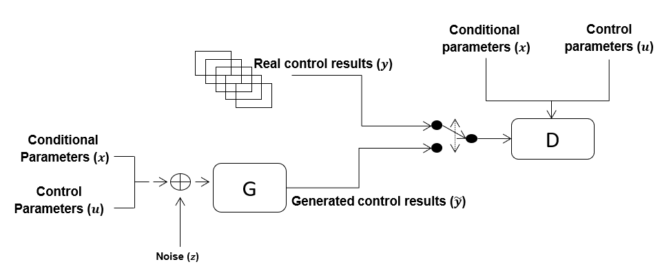
Figure 1. The structure of CGAN models.

Generator ($G$): The input of the generator includes a noise vector ($\mathbf{z}$) consisting of randomly generated float numbers between 0 and 1, and two condition vectors which are the conditional parameters ($\mathbf{x}$) and the control parameters ($\mathbf{u}$). The output of the generator is the vector of control results $\tilde{\mathbf{y}}$. We define the generator as a function $\tilde{\mathbf{y}}=G(\mathbf{z}|\mathbf{x},\mathbf{u})$. The objective of the generator is to generate simulated control results that cannot be distinguished by the discriminator, denoted as follows:

$$\min_{G}\mathbb{E}_{(\mathbf{x},\mathbf{u})\sim p(\mathbf{x},\mathbf{u}),\mathbf{z}\sim p(\mathbf{z})}-D(G(\mathbf{z}|\mathbf{x},\mathbf{u})|\mathbf{x},\mathbf{u})$$

where $p(\mathbf{x},\mathbf{u})$ is the empirical joint distribution of conditional and control parameters in the historical data, $p(\mathbf{z})$ is a multivariate distribution where each dimension follows an independent uniform distribution ${\mathcal{U}(0,1)}$.

Discriminator ($D$): The discriminator also has two inputs. The first part is the two condition vectors $\mathbf{x}$ and $\mathbf{u}$ as the same as the counterpart in the generator. The second part is either a generated control result sample $\tilde{\mathbf{y}}$ or a real control result sample ($\mathbf{y}$). The output of the discriminator is a scalar value. A lower value of the output indicates the discriminator gives a higher likelihood to the control result sample as a generated one. The objective of the discriminator is denoted as follows:

$$\min_{D} \mathbb{E}_{(\mathbf{x},\mathbf{u})\sim p(\mathbf{x},\mathbf{u}),\mathbf{z}\sim p(\mathbf{z})}D(G(\mathbf{z}|\mathbf{x},\mathbf{u})|\mathbf{x},\mathbf{u})$$

$$-\mathbb{E}_{(\mathbf{x},\mathbf{u},\mathbf{y})\sim p(\mathbf{x},\mathbf{u},\mathbf{y})}D(\mathbf{y}|\mathbf{x},\mathbf{u})$$

$$+\lambda\mathbb{E}_{(\mathbf{x},\mathbf{u},\mathbf{y}^{\prime})\sim p(\mathbf{x},\mathbf{u},\mathbf{y}^{\prime})}\Big{[}(||\frac{\Delta D(\mathbf{y}^{\prime}|\mathbf{x},\mathbf{u})}{\Delta\mathbf{y}^{\prime}}||-1)^{2}\Big{]}$$

where the first term minimizes the outputs for simulated samples; the second term maximizes the outputs for real samples; the third term is the gradient penalty loss (Gulrajani et al., 2017) in which $\lambda$ is a hyperparameter often takes the value 10, $\mathbf{y}^{\prime}$ samples uniformly along straight lines between pairs of real and simulated control results with given conditional and control parameters.

Let $r(\mathbf{x},\mathbf{u})$ denote the expected reward given conditional parameters $\mathbf{x}$ and control parameters $\mathbf{u}$. After the $M$ CGAN models are trained, we generate a large number of control result samples using the generators and then utilize the following Monte Carlo approach to calculate $r(\mathbf{x},\mathbf{u})$:

(3) $$r(\mathbf{x},\mathbf{u})=\int\mathrm{p}(\mathbf{y}|\mathbf{x},\mathbf{u})r(\mathbf{y})\mathrm{d}\mathbf{y}\approx\frac{1}{M\cdot N}\sum_{i=1}^{M}\sum_{j=1}^{N}r\big{(}\tilde{\mathbf{y}}_{i}^{j}\big{)}$$

where $N$ is a large integer number, $\tilde{\mathbf{y}}_{i}^{j}=G_{{}_{i}}(\mathbf{z}^{j}|\mathbf{x},\mathbf{u})$ in which $G_{{}_{i}}$ is a trained generator model in the ensemble and $\mathbf{z}^{j}\sim p(\mathbf{z})$.

The main benefit of approximating the dynamics model by ensemble of CGANs based on the above Monte Carlo approach is that we can effectively model any shape of conditional distribution for control results while naturally capturing the dependencies between different dimensions of control results. In this sample-wise way, accurate reward calculation can be achieved.

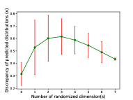
(a)

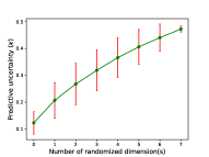
(b)

Figure 2. (a) the mean and standard deviation of the discrepancies between distributions of generated control results with different number of randomized dimension(s) for the inputs of the approximate dynamics model; (b) the mean and standard deviation of the amount of uncertainty for generated control results with different number of randomized dimension(s) for the inputs of the approximate dynamics model.

3.2. Epistemic-uncertainty-penalized reward evaluation

We introduce the epistemic-uncertainty-penalized reward evaluation function that can avoid giving over-estimated rewards to OoD inputs during the learning/searching for the optimal control policy. Notably, over-estimated rewarding for OoD inputs occurs largely due to over-confident predictions are made by the approximate dynamics model when the optimization algorithm is exploring the regions with high epistemic uncertainty, i.e., regions of the industrial process dynamics that are not sufficiently reflected in the historical data. According to previous studies (Lakshminarayanan et al., 2017; Choi et al., 2018), deep generative ensembles will generate predictions with higher uncertainty on OoD inputs and the predictions made by different models within an ensemble are likely to be diverged. Utilizing the above features, MOPO (Yu et al., 2020) proposes to penalize rewards evaluated with higher predictive uncertainty of the deep ensembles, MOReL (Kidambi et al., 2020) proposes to penalize rewards when a large discrepancy between the predicted distributions of the models within the ensemble is observed. However, we find both methods have defects when applying on industrial processes. On one hand, penalizing rewards with higher predictive uncertainty may lead to over-conservative policies because non-OoD inputs with inherently high aleatoric uncertainty will be incorrectly penalized. On the other hand, we observe that discrepancy between the predicted distribution of the models is not monotonically increasing when the input sample is more likely to be an outlier. In fact, we find that the discrepancy starts to decrease at some point where the input sample is sufficiently far away from the historical data distribution (see evidence from figure 2a). As a result, only penalizing rewards based on the discrepancy between predicted distributions cannot avoid giving over-estimated rewards to OoD inputs which are sufficiently far away from the historical data distribution.

To overcome the above problems, we propose the following epistemic-uncertainty-penalized reward evaluation function:

$$r_{p}(\mathbf{x},\mathbf{u})=\begin{cases}(1-\kappa)\cdot r(\mathbf{x},\mathbf{u})&\quad\text{if }\varkappa\leq\epsilon\wedge r(\mathbf{x},\mathbf{u})>0\\ (1+\kappa)\cdot r(\mathbf{x},\mathbf{u})&\quad\text{if }\varkappa\leq\epsilon\wedge r(\mathbf{x},\mathbf{u})\leq 0\\ c&\quad\text{if }\varkappa>\epsilon\end{cases}$$

where $\kappa=\left(\!\begin{array}[]{c}M\\ 2\end{array}\!\right)^{-1}\sum_{i=1}^{M}\sum_{j=i+1}^{M}H^{2}_{i,j}$ is the mean squared Hellinger distance between the distributions of control results generated by the $M$ CGANs, and $\kappa\in(0,1)$; $\varkappa=M^{-1}\sum_{i=1}^{M}||\boldsymbol{\Sigma}_{i}||_{F}$ is the mean norm of the covariance matrices of the generated control results by the $M$ CGANs; $\epsilon$ is a user-defined threshold value which can be set to, e.g., the maximum value of $\varkappa$ calculated on input samples in a validation dataset; $c$ is a constant which denotes an extremely low value to rewards. Specifically, we use $\varkappa$ to measure the uncertainty of generated control results, when it is larger than a threshold value, the epistemic uncertainty will overwhelm, thus we assign an extremely low reward to the input sample to avoid the risk of over-estimated reward estimation. When $\varkappa$ is lower than the threshold value, we penalize rewards only with epistemic uncertainty that is captured by the discrepancy between distributions of generated control results. In this way, the epistemic-uncertainty-penalized reward evaluation function can accurately avoid assigning over-estimated rewards to OoD input samples without leading to over-conservative policies.

To give an intuition about the motivation of our reward evaluation function, we train an ensemble of five CGANs on the a real world industrial dataset (details to be seen in Section 4). Moreover, we replace $n$ dimension(s) of the logged conditional and control inputs in the data with randomly generated values to mimic OoD inputs. With more randomized dimensions, the input sample is more likely to be an outlier. For each input, we generate a large number of control result samples via the five CGANs and measure the discrepancy between the distributions of generated control results of the five CGANs ($\kappa$) and the amount of predictive uncertainty ($\varkappa$). We plot the mean and standard deviation of $\kappa$ and $\varkappa$ with different value of $n$ in figure 2a and figure 2b respectively. As can be seen in Figure 2a, the mean value of $\kappa$ increases along with $n$ when $n\leq 3$, however, it starts to decrease when $n>3$. Therefore, only penalizing rewards with the discrepancy between predicted distributions of control results can potentially assign over-estimated rewards to OoD inputs which are far away from the historical data distribution. However, since the predictive uncertainty will increase as the input is farther away from the historical data distribution as illustrated in Figure 2b, we can effectively avoid assigning over-estimated rewards to those OoD inputs by checking whether the corresponding predictive uncertainty is larger than a threshold value beyond which the epistemic uncertainty overwhelms.

Lastly, with the epistemic-uncertainty-penalized reward evaluation function, we propose the reliable offline model-based optimization framework for discrete industrial process control as follows:

(4) $$\max_{\pi}\mathbb{E}_{\mathbf{x},\mathbf{u}\sim\pi}\Big{[}r_{p}(\mathbf{x},\mathbf{u})\Big{]}$$

For continuous control cases, the proposed reliable optimization framework is given as follows:

(5) $$\max_{\pi}\mathbb{E}_{\mathbf{x}_{0:T},\mathbf{u}_{0:T}\sim\pi}\Big{[}\sum_{t=0}^{T}\gamma^{t}\cdot r_{p}(\mathbf{x}_{t},\mathbf{u}_{t})\Big{]}$$

4. Evaluation on Discrete Control

In this section, we present the experiment in which we applied our proposed framework to optimize the control policy of a discrete control case: the production process of a worm gear production line. Specifically, worm gears, an important component in the steering system of automobiles, are produced using computer numerical control (CNC) machines. Our target is to improve the production quality of worm gears by optimizing the control of CNC machining parameters. In our experiment, we collected a historical dataset from a real worm gear production line with 19760 production records. Each production record consists of three conditional parameters (recorded ambient environment factors during production), four control parameters and seven control result variables (the attributes of produced worm gears for quality check). A worm gear will be checked by a manually defined testing rule decided by the seven control results. The reward for a qualified production is set to 1, otherwise the reward is set to 0.

4.1. Qualitative evaluation

In the qualitative experiments, we aim to answer two questions: 1) Is it really beneficial to use CGANs to approximate the dynamics model than the commonly used GPNs? 2) Is it really necessary to use both the discrepancy between predicted distributions and the amount of predictive uncertainty to penalize rewards?

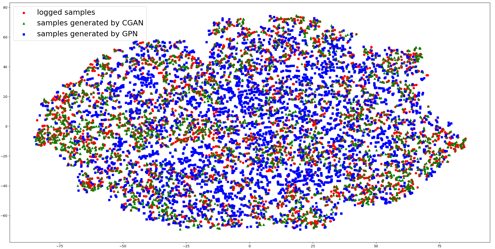
Figure 3. T-SNE 2D visualization for real and generated control result samples

To address the above questions, we firstly split the historical data into a training set and a testing set with the ratio 4:1. We train an ensemble of five CGANs as well as an ensemble of five GPNs to approximate the dynamics model. Specifically, GPNs output a Gaussian distribution over the control results with a diagonal covariance matrix: $p(\mathbf{y}|\mathbf{x},\mathbf{u})\approx\mathcal{N}\big{(}{\boldsymbol{\mu}_{\theta}(\mathbf{x},\mathbf{u}),\boldsymbol{\Sigma}_{\phi}(\mathbf{x},\mathbf{u})}\big{)}$. We can generate control result samples by sampling from the predicted Gaussian distribution.

Then to answer the first question, we use the trained CGANs and GPNs to generate equivalent number of control result samples using the logged conditional and control parameters in the testing set. We use t-SNE (Van der Maaten and Hinton, 2008) to visualize the logged and generated control result samples on a 2D map in Figure 3. As can be seen, the logged control result samples have a much closer pattern with the samples generated by the CGAN models than the ones generated by the GPN models. This is because the CGAN models can reflect the true dynamics of control results by capturing the dependencies between different dimensions of the control results without the assumption for the shape of underlying distribution. It is worth noting that the reward is commonly evaluated based on all dimensions of control results as a whole (e.g., the quality checking rule in the worm gear production line), capturing the dependencies between different dimensions of control results is crucial for the accuracy of reward calculation. Therefore, using CGANs to approximate the dynamics model is much more reliable than GPNs.

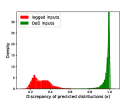
(a)

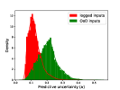
(b)

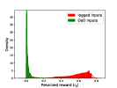
(c)

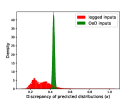
(d)

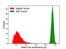
(e)

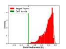
(f)

Figure 4. (a,b,c): the distribution of $\kappa$, $\varkappa$ and $r_{p}$ for the logged inputs compared with the counterpart for the OoD inputs with only control parameter values are randomly generated; (d,e,f): the distribution of $\kappa$, $\varkappa$ and $r_{p}$ for the logged inputs compared with the counterpart for the OoD inputs whose conditional and control parameters are all randomly generated.

To answer the second question, we evaluate the distribution discrepancy ($\kappa$), the predictive uncertainty ($\varkappa$) and the penalized rewards ($r_{p}$) based on the generated control results by the ensemble of CGANs given three set of inputs: 1) the first set is the logged conditional and control parameters in the testing data; 2) the second set is the logged conditional parameters in the testing data, but combined with randomly generated control parameters to mimic OoD inputs; 3) the third set consists of OoD inputs whose conditional and control parameters are all randomly generated. We compare the empirical distribution of $\kappa$, $\varkappa$ and $r_{p}$ for the logged inputs and the OoD inputs in the second set in Figure 4a, 4b and 4c respectively. Furthermore, we compare the empirical distribution of $\kappa$, $\varkappa$ and $r_{p}$ for the logged inputs and the OoD inputs in the third set in Figure 4d, 4e and 4f respectively. As can be seen, when given OoD inputs with only control parameters are randomly generated, we cannot perfectly distinguish OoD inputs from logged inputs using predictive uncertainty of control results (Figure 4b), but can distinguish easily using discrepancy between predicted distributions of control results (Figure 4a). When given OoD inputs whose conditional and control parameters are all randomly generated, we cannot perfectly distinguish OoD inputs from logged inputs using discrepancy between predicted distributions of control results (Figure 4d), but can distinguish easily using predictive uncertainty (Figure 4e). However, we can easily distinguish OoD inputs from logged inputs using our epistemic-uncertainty-penalized rewards in both scenarios (Figure 4c and 4f). From the above results, we can conclude that to accurately avoid giving over-estimated rewards to OoD inputs, it is necessary to use both the discrepancy between predicted distributions and the amount of predictive uncertainty to penalize rewards.

4.2. Quantitative evaluation

We utilize the optimization framework in Equation 4 to search for the optimal control parameters. For simplicity, given observed conditional parameters $\mathbf{x}$, we can convert the optimization problem as follows:

(6) $$\mathbf{u}^{*}=\arg\max_{\mathbf{u}\in\mathcal{A}}f(\mathbf{u}|\mathbf{x})$$

where $\mathcal{A}$ is the value space of control parameters, $f(\mathbf{u}|\mathbf{x})=r_{p}(\mathbf{x},\mathbf{u})$. Technically, we derive the (near) optimal control parameters $\mathbf{u}^{*}$ via Bayesian optimization.

4.2.1. Baselines

We consider the following four baselines to demonstrate the benefits of our proposed framework:

Baseline1: We ignore the epistemic-uncertainty-penalized function to evaluate rewards. This means that we replace $f(\mathbf{u}|\mathbf{x})$ in Equation 6 with $f_{1}(\mathbf{u}\mid\mathbf{x})$ such that $f_{1}(\mathbf{u}|\mathbf{x})=r(\mathbf{x},\mathbf{u})$.

Baseline2: We replace ensemble of CGANs by ensemble of GPNs to approximate the dynamics model and use the same epistemic-uncertainty-penalized function to evaluate rewards. This means that we replace $\tilde{\mathbf{y}}^{j}_{i}$ in Equation 3 by samples from the predicted distributions of control results by GPNs.

Baseline3: We use the MOReL (Kidambi et al., 2020) style function to penalize rewards. More specifically, let disc$(\mathbf{x},\mathbf{u})=\max_{i,j}H^{2}_{i,j}$ be the maximum discrepancy for the predicted distributions of control results, we replace $f(\mathbf{u}|\mathbf{x})$ with $f_{3}(\mathbf{u}|\mathbf{x})$ such that:

$$f_{3}(\mathbf{u}|\mathbf{x})=\begin{cases}r(\mathbf{x},\mathbf{u})&\quad\text{if }\text{disc}(\mathbf{x},\mathbf{u})\leq\text{threshold}\\ 0&\quad\text{otherwise}\end{cases}$$

where the threshold is a user-defined hyperparameter. As can be seen, MOReL penalizes rewards only based on discrepancy of predicted distributions of control results.

Baseline4: We use the MOPO (Yu et al., 2020) style function to penalize rewards. We replace $f(\mathbf{u}|\mathbf{x})$ with $f_{4}(\mathbf{u}|\mathbf{x})$ such that:

$$f_{4}(\mathbf{u}|\mathbf{x})=r(\mathbf{x},\mathbf{u})-\lambda\max_{i=1,...,M}||\boldsymbol{\Sigma}_{i}||_{F}$$

where $\lambda$ is a user-defined hyperparameter. As can be seen, MOPO penalizes rewards only based on the amount of uncertainty for predicted distributions of control results.

4.2.2. Evaluation metrics and results

The learned policy by our proposed method has been deployed on the production line and showed improved qualified rate of production than the behaviour policy. To compare the performance with the baselines, the ideal way is to run the policies learned by different methods on the production line for sufficiently long time and compare the average reward (qualified rate) of production using different policies. However, it is infeasible to do so due to technical and safety issues. As a result, we use off-policy evaluation (OPE) methods (Precup, 2000; Dudík et al., 2011; Dudík et al., 2014; Hanna et al., 2019) to compare the performance of different policies. Specifically, we train the approximate dynamics models (ensemble of CGANs and GPNs) on the training data and apply OPE on the testing data. Concretely, we compare the metrics calculated by the following four commonly used OPE methods: Direct Method (DM), Inverse Propensity Score (IPS), Weighted Importance Sampling (WIS) and Doubly Robust (DR) estimator. The implementation details of the four OPE methods are given in A.2.

In Table 1, we present the calculated metrics for different policies using the four OPE methods. As can be seen, the control policy learned by our proposed method achieves the best metric on three out of four OPE methods. In the metrics for IPS and DR, our method outperforms the baselines with a clear margin. The only exception for which our method does not achieve the best metric is DM. We believe this is because the DM method suffers from high bias in our case since we cannot train an accurate model to directly predict rewards given conditional and control parameters as inputs.

Table 1. The calculated metrics for different policies using different OPE methods in the worm gear production line case.

	DM	IPS	WIS	DR
Baseline1	0.80	0.02	0.85	0.80
Baseline2	0.63	0.45	0.86	0.61
Baseline3	0.64	0.38	0.80	0.62
Baseline4	0.83	0.10	0.75	0.84
Our method	0.65	7.67	0.86	0.94

5. Evaluation on Continuous Control

In this section, we present the experiment in which we applied our proposed framework on the industrial benchmark (IB), a public available simulator with properties inspired by real industrial systems with continuous control (Hein et al., 2017a). According to the authors, the process of searching for an optimal control policy on the IB is to resemble the task of finding optimal valve settings for gas turbines or optimal pitch angles and rotor speeds for wind turbines.

Algorithm 1 Reliable offline model-based optimization instantiation with DDPG for industrial process control

0:  A historical dataset $\mathcal{D}$, the reward function $r(\mathbf{y})$

1:  Train on the historical dataset $\mathcal{D}$ an ensemble of $M$ CGAN models, $\{G_{i}\}_{i=1}^{M}$

2:  Randomly initialize the critic network $Q(\mathbf{x},\mathbf{u})$ and policy (actor) network $\pi(\mathbf{x})$

3:  Initialize target network $Q^{\prime}(\mathbf{x},\mathbf{u})$ and $\pi^{\prime}(\mathbf{x})$ with same weights with $Q(\mathbf{x},\mathbf{u})$ and $\pi(\mathbf{x})$ respectively

4:  Initialize replay buffer $R$

5:  for episode=1,K do

6:     Initialize a random process $\mathcal{N}$ for action exploration

7:     Sample an initial conditional parameters $\mathbf{x}_{0}$ from $\mathcal{D}$

8:     for $t=1,T$ do

9:        Select control parameters $\mathbf{u}_{t}=\pi(\mathbf{x}_{t})+\mathcal{N}_{t}$ according to the current policy and exploration noise

10:        for $i=1,M$ do

11:           Generate $N$ control result samples by $\tilde{\mathbf{y}}_{i}^{j}=G_{i}(\mathbf{z}_{j}|\mathbf{x}_{t},\mathbf{u}_{t})$ where $\mathbf{z}_{j}\sim p(\mathbf{z})$, $j=1,2,...,N$

12:        end for

13:         Compute the epistemic-uncertainty-penalized reward $r_{p}(\mathbf{x}_{t},\mathbf{u}_{t})$.

14:        Randomly pick a sample $\mathbf{y}_{t}$ from $\{\tilde{\mathbf{y}}_{i}^{j}\}_{i=1:M}^{j=1:N}$ and set $\mathbf{x}_{t+1}=\mathbf{y}_{t}$.

15:        Add sample $\big{(}\mathbf{x}_{t},\mathbf{u}_{t},r_{p}(\mathbf{x}_{t},\mathbf{u}_{t}),\mathbf{x}_{t+1}\big{)}$ to $R$

16:        Use DDPG to update $Q,\pi$ and $Q^{\prime},\pi^{\prime}$

17:     end for

18:  end for

Control policies in the IB need to specify changes $\Delta v$, $\Delta g$ and $\Delta s$ in three observable steering variables $v$ (velocity), $g$ (gain) and $s$ (shift). In our experiment, we set the conditional parameters at a time $t$ as $\mathbf{x}_{t}=[v_{t},g_{t},s_{t},c_{t},f_{t}]$ where $c_{t}\geq 0$ (consumption) and $f_{t}\geq 0$ (fatigue) are two reward relevant variables; the control parameters at time $t$ as $\mathbf{u}_{t}=[\Delta v_{t},\Delta g_{t},\Delta s_{t}]$; the control results of time $t$ as $\mathbf{y}_{t}=[v_{t+1},g_{t+1},s_{t+1},c_{t+1},f_{t+1}]$. The reward of time $t$ is calculated as $r(\mathbf{y}_{t})=-c_{t+1}-3f_{t+1}$.

We generate two sets of historical data using two behaviour policies: a random behaviour policy and a safe behaviour policy. Specifically, the random behaviour policy will set control parameters which are randomly sampled from the value space. The safe behaviour policy will keep the velocity and gain only in a medium range using a conservative strategy such that a very limited value space for velocity and gain will be covered. We use each behaviour policy to simulate 300 trajectories of length 100 as the historical data. For each historical dataset, we apply our proposed offline model-based optimization framework in Equation 5 to learn the optimal control policy. Specifically, we use DDPG (Lillicrap et al., 2016) as the backbone of the underlying RL algorithm, and the implementation details are given in Algorithm 1. Using the same DDPG backbone, we also compare the performance of our learned policies with same baselines in the previous section. To get a fair comparison, on each historical dataset we run the training algorithm for 1500 episodes with 5 random seeds for each method. We report the undiscounted reward of the selected policies on the IB simulator averaged over the last 100 training episodes with the 5 random seeds, $\pm$ standard deviation. The results are reported in Table 2 in which the performance of the behaviour policies is also included. As can be seen, our proposed method achieves the highest average reward on both scenarios with a clear margin. We also find that our proposed method is the only one which can achieve better performance than the behaviour policy in both scenarios.

To give more insights, we find the performance of Baseline1 is much worse when trained on the data generated by the safe behaviour policy. This means that the policies leaned by Baseline1 that ignores the epistemic-uncertainty-penalized reward function, cannot avoid outputting OoD control parameters. This also happens to Baseline3, which means that penalizing rewards with the MOReL style function that only based on the discrepancy between predicted distributions can still output OoD control parameters. For Baseline2, we find it fails to achieve good performance in both scenarios. This is because using ensemble of GPNs cannot capture the true dynamics of the underlying process. For Baseline4, we find that its performance on both scenarios is close to the behaviour policy. This means that penalizing rewards with the MOPO style function that only based on the predictive uncertainty of control results will make the learned policies over-conservative. To sum up, we can conclude that the epistemic-uncertainty-penalized reward evaluation function is better at handling the distribution shift problem than the baselines, and the usage of CGANs can also largely improve the reliability of learned policies compared with GPNs.

Table 2. The performance of the behaviour policy and control policies learned from historical data by different methods on the IB.

	Random	Safe
behaviour policy	-247.0 $\pm$ 32.8	-216.3 $\pm$ 12.0
Baseline1	-254.2 $\pm$ 47.4	-436.3 $\pm$ 54.9
Baseline2	-270.1 $\pm$ 25.9	-319.8 $\pm$ 34.3
Baseline3	-258.4 $\pm$ 21.7	-344.4 $\pm$ 10.3
Baseline4	-239.0 $\pm$ 15.4	-222.8 $\pm$ 10.4
Our method	-207.3 $\pm$ 13.1	-201.1 $\pm$ 11.2

6. Related Work

Learning optimal control policies from offline data is known to suffer from the distribution shift problem. Several techniques have been proposed to tackle the problem. For example, one approach is to constrain the learned policy to be closer to the behaviour policy which is adopted by many model-free offline RL algorithms (Fujimoto et al., 2019; Jaques et al., 2019; Kumar et al., 2019; Nachum et al., 2019; Peng et al., 2019; Wu et al., 2019; Siegel et al., 2020). Another approach is to train a conservative dynamics model or critic that minimizes the predictions on OoD inputs for offline model-based optimization (Trabucco et al., 2021; Yu et al., 2021). (Kumar and Levine, 2020) use a CGAN model to fit an inverse map from the rewards to inputs so as to discourage too much departure of optimized inputs from the training data. A more common approach for offline model-based optimization is to utilize uncertainty quantification to evaluate the risk of giving overestimated rewards to OoD inputs (Chua et al., 2018; Yu et al., 2020; Kidambi et al., 2020; Argenson and Dulac-Arnold, 2020). To quantify the uncertainty, the choice of dynamics model is crucial. Many recent works utilize ensemble of GPNs (Lakshminarayanan et al., 2017) which assume that different dimensions of the outputs are conditionally independent as the dynamics model. However, this assumption rarely holds in real applications. As a result, (Zhang et al., 2020) propose an autoregressive dynamics model in which the distribution of one dimension in the output depends on the previous dimension. Our work also takes the uncertainty-quantification approach, but with the difference that we leverage ensemble of CGANs as the dynamics model to produce more realistic control result samples for reliable uncertainty quantification.

Data-driven control policy learning have been applied in industrial systems for more than decades (Hoskins and Himmelblau, 1992; Schlang et al., 1999; Runkler et al., 2003; Schaefer et al., 2007; Hartmann and Runkler, 2008). However, most of them focus on online scenarios where there is a simulator of the industrial process to provide control feedback (Nian et al., 2020). In practice, building accurate simulation models for industrial systems is often very costly or infeasible. Learning control policies for industrial processes from offline data has been recently explored. For example, a particle swarm optimization-based algorithm is combined with a planning-based strategy for offline control in the Industrial Benchmark (Hein et al., 2017b). A generic programming-based approach is proposed to generate interpretable control policies for industrial systems from offline data (Hein et al., 2018). Similar to our work is (Depeweg et al., 2018) in which a risk-sensitive model-based offline RL algorithm based on Bayesian neural networks is proposed to handle noisy industrial systems. Different from previous approaches, our proposed reliable offline model-based optimization framework is general to both the discrete and continuous control cases, and is agnostic to the optimization algorithm being used.

7. Conclusion

In this work, we extend the current success of offline model-based optimization to real-world industrial process control problems by 1) learning an ensemble of CGANs to approximate the dynamics model in which the aleatoric uncertainty, dependencies between different dimensions and the non-Gaussian dynamics of control results are well captured via a Monte Carlo approach for reliable reward calculation; 2) proposing an epistemic-uncertainty-penalized reward evaluation function which can effectively avoid assigning over-estimated rewards to OoD inputs. Through the experiments on a discrete control case and a continuous control case, we show both the proposed approximate dynamics model and the reward evaluation function are crucial to improve the reliability and performance of offline learned control policies for industrial processes.

Appendix A Appendix

A.1. Calculation of Squared Hellinger Distance

For convenience, we calculate the squared Hellinger distance via a closed form expression by assuming the generated control results follow multivariate Gaussian distributions. Note that this does not affect the fact the CGANs can capture non-Gaussian conditional distribution of control results. Specifically, let $\boldsymbol{\mu}_{i}$ and $\boldsymbol{\Sigma}_{i}$ denote the empirical mean and covariance of control result samples generated by a generator $G_{i}$, we compute the squared Hellinger distance between a pair of predicted distributions of two CGANs as follows :

$$H^{2}_{i,j} = 1-\frac{\det(\boldsymbol{\Sigma}_{i})^{\frac{1}{4}}\det(\boldsymbol{\Sigma}_{j})^{\frac{1}{4}}}{\det(\frac{\boldsymbol{\Sigma}_{i}+\boldsymbol{\Sigma}_{j}}{2})^{\frac{1}{2}}}\times\exp\left\{-{\frac{1}{8}}(\boldsymbol{\mu}_{i}-\boldsymbol{\mu}_{j})^{T}\left({\frac{\boldsymbol{\Sigma}_{i}+\boldsymbol{\Sigma}_{j}}{2}}\right)^{-1}(\boldsymbol{\mu}_{i}-\boldsymbol{\mu}_{j})\right\}$$

A.2. Implementation details of OPE methods

Direct Method (DM): The DM estimator forms an estimate $\hat{r}(\mathbf{x}_{k},\mathbf{u}^{*}_{k})$ of the expected reward given the conditional and control parameters, the expected reward of the proposed policy is then estimated by:

$$\hat{V}^{\pi}_{\text{DM}}=\frac{1}{n}\sum_{k=1}^{n}\hat{r}(\mathbf{x}_{k},\mathbf{u}^{*}_{k})$$

where $n$ is the number of production records in the testing data. We train a multiple layer perception (MLP) network on the training data as the predictive model to estimate $\hat{r}(\mathbf{x}_{k},\mathbf{u}^{*}_{k})$. DM estimator can suffer from high bias since it highly relies on the accuracy of the predictive model.

Inverse Propensity Score (IPS): The IPS estimator evaluates the average reward of a policy by fixing the distribution mismatch between logging controls and policy controls:

$$\hat{V}^{\pi}_{\text{IPS}}=\frac{1}{n}\sum_{k=1}^{n}\frac{p_{\pi}(\mathbf{u}_{k}|\mathbf{x}_{k})}{p_{\text{log}}(\mathbf{u}_{k}|\mathbf{x}_{k})}r(\mathbf{y}_{k})$$

where $p_{\text{log}}(\mathbf{u}_{k}|\mathbf{x}_{k})$ is the probability of taking control parameters $\mathbf{u}_{k}$ given conditional parameters $\mathbf{x}_{k}$ for the logging policy, $p_{\pi}(\mathbf{u}_{k}|\mathbf{x}_{k})$ is the corresponding probability for the learned policy. Similar to (Hanna et al., 2019), we estimate $p_{\text{log}}(\mathbf{u}_{k}|\mathbf{x}_{k})$ by fitting a GPN on the historical dataset. $p_{\pi}(\mathbf{u}_{k}|\mathbf{x}_{k})$ is estimated by fitting a Gaussian distribution for 10 output control parameters generated by Bayesian optimization each with different random seeds. The IPS estimator can suffer from large variance especially when the log policy differs significantly from the policy to be evaluated (Horvitz and Thompson, 1952; Dudík et al., 2011).

Weighted Importance Sampling (WIS): Let $w_{k}=\frac{p_{\pi}(\mathbf{u}_{k}|\mathbf{x}_{k})}{p_{\text{log}}(\mathbf{u}_{k}|\mathbf{x}_{k})}$ be the importance weight, the WIS estimator evaluates the average reward of a policy as follows:

$$\hat{V}^{\pi}_{\text{WIS}}=\frac{\sum_{k=1}^{n}w_{k}r(\mathbf{y}_{k})}{\sum_{k=1}^{n}w_{k}}$$

As stated in (Precup, 2000), the WIS estimator is often more stable in practice than the IPS estimator.

Doubly Robust (DR) estimator: The DR estimator takes the advantage of both the DM estimates and the importance weights to provide a more robust evaluation of the expected reward for a proposed policy. Specifically, we adopt the DR estimator in (Dudík et al., 2014) as shown below:

$$\hat{V}^{\pi}_{\text{DR}}=\frac{1}{n}\sum_{k=1}^{n}\big{[}\hat{r}(\mathbf{x}_{k},\mathbf{u}^{*}_{k})+w_{k}\big{(}r(\mathbf{y}_{k})-\hat{r}(\mathbf{x}_{k},\mathbf{u}_{k})\big{)}\big{]}$$

where $\hat{r}(\mathbf{x}_{k},\mathbf{u}_{k})$ is the expected reward for a log control using the predictive model in the DM estimator.

A.3. Implementation Details of Behaviour Policies in the IB

In the random behaviour policy, we set $\Delta v=u_{v}$, $\Delta g=u_{g}$, $\Delta s=u_{s}$ such that $u_{v},u_{g},u_{s}\sim\mathcal{U}(-1,1)$. In the safe behavior policy, $\Delta v$, $\Delta g$, $\Delta s$ are sampled according to the following rule:

$$\Delta v=\begin{cases}z_{v}&\quad\text{if }v_{t}<40\\ -z_{v}&\quad\text{if }v_{t}>60\\ u_{v}&\quad\text{otherwise,}\end{cases}$$

$$\Delta g=\begin{cases}z_{g}&\quad\text{if }g_{t}<40\\ -z_{g}&\quad\text{if }g_{t}>60\\ u_{g}&\quad\text{otherwise,}\end{cases}$$

$\Delta s=u_{s}$, where $z_{v},z_{g}\sim\mathcal{N}(0.5,\frac{1}{\sqrt{3}})$, and $u_{v},u_{g},u_{s}\sim\mathcal{U}(-1,1)$. The velocity $v_{t}$ and gain $g_{t}$ can take values in $[0,100]$. Therefore, the safe behaviour policy will try to keep these values only in the medium range given by the interval $[40,60]$. Because of this, large parts of the state space will be unobserved.

A.4. Hyperparameters

For both the worm gear production line and the IB, we use 2 layer MLPs with 64 hidden dimensions as the generator and the discriminator for the CGANs. Each CGAN model is trained with 3000 epochs. For the GPN models, we do a hyperparameter search with hidden layers from 1 to 4, hidden dimensions from 8 to 256, epochs from 50 to 200 to get the lowest negative log likelihood on the testing data. $M$ is set to 5; $N$ (number of control result samples to be simulated by each CGAN or GPN) is set to 1000; $\epsilon$ is set to the maximum value of $\varkappa$ calculated on input samples in the testing data; the threshold for Baseline3 is set to the maximum value of $\text{disc}(\mathbf{x},\mathbf{u})$ calculated on input samples in the testing data. For the worm gear production line case, $c$ is set to 0, $\lambda$ in Baseline4 is set to $1$ for best performance. For the IB case, $c$ is set to -2000, $\lambda$ in Baseline4 is set to $1000$ for best performance. Furthermore, we use 2 layer MLPs with 64 hidden dimensions as the policy and critic networks in the DDPG alogrithm.

References

- (1)
- Argenson and Dulac-Arnold (2020) Arthur Argenson and Gabriel Dulac-Arnold. 2020. Model-based offline planning. arXiv preprint arXiv:2008.05556 (2020).
- Choi et al. (2018) Hyunsun Choi, Eric Jang, and Alexander A Alemi. 2018. Waic, but why? generative ensembles for robust anomaly detection. arXiv preprint arXiv:1810.01392 (2018).
- Chua et al. (2018) Kurtland Chua, Roberto Calandra, Rowan McAllister, and Sergey Levine. 2018. Deep reinforcement learning in a handful of trials using probabilistic dynamics models. In Proceedings of the 32nd International Conference on Neural Information Processing Systems. 4759–4770.
- Deisenroth et al. (2013) Marc Peter Deisenroth, Dieter Fox, and Carl Edward Rasmussen. 2013. Gaussian processes for data-efficient learning in robotics and control. IEEE transactions on pattern analysis and machine intelligence 37, 2 (2013), 408–423.
- Depeweg et al. (2017) S Depeweg, JM Hernández-Lobato, F Doshi-Velez, and S Udluft. 2017. Learning and policy search in stochastic dynamical systems with Bayesian neural networks. In 5th International Conference on Learning Representations, ICLR 2017. 1–14.
- Depeweg et al. (2018) Stefan Depeweg, Jose-Miguel Hernandez-Lobato, Finale Doshi-Velez, and Steffen Udluft. 2018. Decomposition of uncertainty in Bayesian deep learning for efficient and risk-sensitive learning. In International Conference on Machine Learning. PMLR, 1184–1193.
- Dudík et al. (2014) Miroslav Dudík, Dumitru Erhan, John Langford, and Lihong Li. 2014. Doubly robust policy evaluation and optimization. Statist. Sci. 29, 4 (2014), 485–511.
- Dudík et al. (2011) Miroslav Dudík, John Langford, and Lihong Li. 2011. Doubly robust policy evaluation and learning. In Proceedings of the 28th International Conference on International Conference on Machine Learning. 1097–1104.
- Fu et al. (2020) Justin Fu, Aviral Kumar, Ofir Nachum, George Tucker, and Sergey Levine. 2020. D4rl: Datasets for deep data-driven reinforcement learning. arXiv preprint arXiv:2004.07219 (2020).
- Fujimoto et al. (2019) Scott Fujimoto, David Meger, and Doina Precup. 2019. Off-policy deep reinforcement learning without exploration. In International Conference on Machine Learning. PMLR, 2052–2062.
- Goodfellow et al. (2014) Ian Goodfellow, Jean Pouget-Abadie, Mehdi Mirza, Bing Xu, David Warde-Farley, Sherjil Ozair, Aaron Courville, and Yoshua Bengio. 2014. Generative adversarial nets. Advances in neural information processing systems 27 (2014).
- Gulrajani et al. (2017) Ishaan Gulrajani, Faruk Ahmed, Martin Arjovsky, Vincent Dumoulin, and Aaron Courville. 2017. Improved training of wasserstein gans. arXiv preprint arXiv:1704.00028 (2017).
- Hanna et al. (2019) Josiah Hanna, Scott Niekum, and Peter Stone. 2019. Importance sampling policy evaluation with an estimated behavior policy. In International Conference on Machine Learning. PMLR, 2605–2613.
- Hartmann and Runkler (2008) Stephan A Hartmann and Thomas A Runkler. 2008. Online optimization of a color sorting assembly buffer using ant colony optimization. In Operations Research Proceedings 2007. Springer, 415–420.
- Hein et al. (2017a) Daniel Hein, Stefan Depeweg, Michel Tokic, Steffen Udluft, Alexander Hentschel, Thomas A Runkler, and Volkmar Sterzing. 2017a. A benchmark environment motivated by industrial control problems. In 2017 IEEE Symposium Series on Computational Intelligence (SSCI). IEEE, 1–8.
- Hein et al. (2018) Daniel Hein, Steffen Udluft, and Thomas A Runkler. 2018. Interpretable policies for reinforcement learning by genetic programming. Engineering Applications of Artificial Intelligence 76 (2018), 158–169.
- Hein et al. (2017b) Daniel Hein, Steffen Udluft, Michel Tokic, Alexander Hentschel, Thomas A Runkler, and Volkmar Sterzing. 2017b. Batch reinforcement learning on the industrial benchmark: First experiences. In 2017 International Joint Conference on Neural Networks (IJCNN). IEEE, 4214–4221.
- Horvitz and Thompson (1952) Daniel G Horvitz and Donovan J Thompson. 1952. A generalization of sampling without replacement from a finite universe. Journal of the American statistical Association 47, 260 (1952), 663–685.
- Hoskins and Himmelblau (1992) JC Hoskins and DM Himmelblau. 1992. Process control via artificial neural networks and reinforcement learning. Computers & chemical engineering 16, 4 (1992), 241–251.
- Jaques et al. (2019) Natasha Jaques, Asma Ghandeharioun, Judy Hanwen Shen, Craig Ferguson, Agata Lapedriza, Noah Jones, Shixiang Gu, and Rosalind Picard. 2019. Way off-policy batch deep reinforcement learning of implicit human preferences in dialog. arXiv preprint arXiv:1907.00456 (2019).
- Kamthe and Deisenroth (2018) Sanket Kamthe and Marc Deisenroth. 2018. Data-efficient reinforcement learning with probabilistic model predictive control. In International conference on artificial intelligence and statistics. PMLR, 1701–1710.
- Kidambi et al. (2020) Rahul Kidambi, Aravind Rajeswaran, Praneeth Netrapalli, and Thorsten Joachims. 2020. MOReL: Model-Based Offline Reinforcement Learning. In NeurIPS.
- Kumar et al. (2019) Aviral Kumar, Justin Fu, Matthew Soh, George Tucker, and Sergey Levine. 2019. Stabilizing Off-Policy Q-Learning via Bootstrapping Error Reduction. Advances in Neural Information Processing Systems 32 (2019), 11784–11794.
- Kumar and Levine (2020) Aviral Kumar and Sergey Levine. 2020. Model Inversion Networks for Model-Based Optimization. Advances in Neural Information Processing Systems 33 (2020).
- Lakshminarayanan et al. (2017) Balaji Lakshminarayanan, Alexander Pritzel, and Charles Blundell. 2017. Simple and scalable predictive uncertainty estimation using deep ensembles. Advances in neural information processing systems 30 (2017).
- Levine et al. (2020) Sergey Levine, Aviral Kumar, George Tucker, and Justin Fu. 2020. Offline reinforcement learning: Tutorial, review, and perspectives on open problems. arXiv preprint arXiv:2005.01643 (2020).
- Lillicrap et al. (2016) Timothy P Lillicrap, Jonathan J Hunt, Alexander Pritzel, Nicolas Heess, Tom Erez, Yuval Tassa, David Silver, and Daan Wierstra. 2016. Continuous control with deep reinforcement learning.. In ICLR.
- Mirza and Osindero (2014) Mehdi Mirza and Simon Osindero. 2014. Conditional generative adversarial nets. arXiv preprint arXiv:1411.1784 (2014).
- Nachum et al. (2019) Ofir Nachum, Bo Dai, Ilya Kostrikov, Yinlam Chow, Lihong Li, and Dale Schuurmans. 2019. Algaedice: Policy gradient from arbitrary experience. arXiv preprint arXiv:1912.02074 (2019).
- Nian et al. (2020) Rui Nian, Jinfeng Liu, and Biao Huang. 2020. A review on reinforcement learning: Introduction and applications in industrial process control. Computers & Chemical Engineering 139 (2020), 106886.
- Peng et al. (2019) Xue Bin Peng, Aviral Kumar, Grace Zhang, and Sergey Levine. 2019. Advantage-weighted regression: Simple and scalable off-policy reinforcement learning. arXiv preprint arXiv:1910.00177 (2019).
- Precup (2000) Doina Precup. 2000. Eligibility traces for off-policy policy evaluation. Computer Science Department Faculty Publication Series (2000), 80.
- Rasmussen (2003) Carl Edward Rasmussen. 2003. Gaussian processes in machine learning. In Summer school on machine learning. Springer, 63–71.
- Runkler et al. (2003) TA Runkler, E Gerstorfer, M Schlang, E Jünnemann, and J Hollatz. 2003. Modelling and optimisation of a refining process for fibre board production. Control engineering practice 11, 11 (2003), 1229–1241.
- Schaefer et al. (2007) Anton Maximilian Schaefer, Daniel Schneegass, Volkmar Sterzing, and Steffen Udluft. 2007. A neural reinforcement learning approach to gas turbine control. In 2007 International Joint Conference on Neural Networks. IEEE, 1691–1696.
- Schlang et al. (1999) Martin Schlang, Björn Feldkeller, Bernhard Lang, Thomas Poppe, and Thomas Runkler. 1999. Neural computation in steel industry. In 1999 European Control Conference (ECC). IEEE, 2922–2927.
- Shahriari et al. (2015) Bobak Shahriari, Kevin Swersky, Ziyu Wang, Ryan P Adams, and Nando De Freitas. 2015. Taking the human out of the loop: A review of Bayesian optimization. Proc. IEEE 104, 1 (2015), 148–175.
- Siegel et al. (2020) Noah Y Siegel, Jost Tobias Springenberg, Felix Berkenkamp, Abbas Abdolmaleki, Michael Neunert, Thomas Lampe, Roland Hafner, Nicolas Heess, and Martin Riedmiller. 2020. Keep doing what worked: Behavioral modelling priors for offline reinforcement learning. arXiv preprint arXiv:2002.08396 (2020).
- Sivanandam and Deepa (2008) SN Sivanandam and SN Deepa. 2008. Genetic algorithms. In Introduction to genetic algorithms. Springer, 15–37.
- Spielberg et al. (2017) SPK Spielberg, RB Gopaluni, and PD Loewen. 2017. Deep reinforcement learning approaches for process control. In 2017 6th international symposium on advanced control of industrial processes (AdCONIP). IEEE, 201–206.
- Sutton and Barto (2018) Richard S Sutton and Andrew G Barto. 2018. Reinforcement learning: An introduction. MIT press.
- Trabucco et al. (2021) Brandon Trabucco, Aviral Kumar, Xinyang Geng, and Sergey Levine. 2021. Conservative objective models for effective offline model-based optimization. In International Conference on Machine Learning. PMLR, 10358–10368.
- Van der Maaten and Hinton (2008) Laurens Van der Maaten and Geoffrey Hinton. 2008. Visualizing data using t-SNE. Journal of machine learning research 9, 11 (2008).
- Wu et al. (2019) Yifan Wu, George Tucker, and Ofir Nachum. 2019. Behavior regularized offline reinforcement learning. arXiv preprint arXiv:1911.11361 (2019).
- Yu et al. (2021) Tianhe Yu, Aviral Kumar, Rafael Rafailov, Aravind Rajeswaran, Sergey Levine, and Chelsea Finn. 2021. Combo: Conservative offline model-based policy optimization. arXiv preprint arXiv:2102.08363 (2021).
- Yu et al. (2020) Tianhe Yu, Garrett Thomas, Lantao Yu, Stefano Ermon, James Y Zou, Sergey Levine, Chelsea Finn, and Tengyu Ma. 2020. MOPO: Model-based Offline Policy Optimization. Advances in Neural Information Processing Systems 33 (2020), 14129–14142.
- Zhang et al. (2020) Michael R Zhang, Thomas Paine, Ofir Nachum, Cosmin Paduraru, George Tucker, Mohammad Norouzi, et al. 2020. Autoregressive Dynamics Models for Offline Policy Evaluation and Optimization. In International Conference on Learning Representations.