Radiative first-order phase transitions to next-to-next-to-leading-order

Abstract

We develop new perturbative tools to accurately study radiatively-induced first-order phase transitions. Previous perturbative methods have suffered internal inconsistencies and been unsuccessful in reproducing lattice data, which is often attributed to infrared divergences of massless modes (the Linde problem). We employ a consistent power counting scheme to perform calculations, and compare our results against lattice data. We conclude that the consistent expansion removes many previous issues, and indicates that the infamous Linde problem is not as big a factor in these calculations as previously thought.

I Introduction

A first-order phase transition at the electroweak scale would have far-reaching consequences for the early universe, for example by triggering baryogenesis Kuzmin et al. (1985), and thereby explain the matter-antimatter asymmetry. In general such a violent transition would echo across the universe; leaving a stochastic background of gravitational waves in its wake. This makes searching for the telltale spectral shape Hindmarsh et al. (2017) a key scientific objective of current and planned gravitational wave observatories Arzoumanian et al. (2020); Amaro-Seoane et al. (2017); Kawamura et al. (2011); Ruan et al. (2020); El-Neaj et al. (2020). Besides giving clear evidence for a first-order transition, a detected signal would constrain models of dark matter Schwaller (2015); Croon et al. (2018), baryogenesis Vaskonen (2017), inflation Addazi et al. (2019) and grand unification Croon et al. (2019).

Yet current tools have a hard time making reliable predictions, particularly so for phase transitions which are radiatively induced, where perturbative calculations often cannot distinguish between first-order, second-order, and crossover transitions. Alternatively, lattice Monte-Carlo simulations can provide quantitatively reliable predictions, up to (small) statistical uncertainties. But they are slow, typically requiring thousands of CPU hours to accurately determine the thermodynamics of a single parameter point.

As a consequence, even with its problems, perturbation theory is the only tool capable of scanning the high-dimensional parameter spaces of theories beyond the Standard Model, which makes it imperative to put perturbative calculations on a solid footing.

In this paper we vie to do just that. In particular, we construct a new perturbative expansion for models with radiatively-induced phase transitions. Furthermore, to ensure accuracy we compare the results with lattice data. In the process we draw attention to prevailing problems with standard perturbative approaches in this context (for an overview see Ref. Croon et al. (2021)).

II Theoretical challenges

Consistent calculations of physical observables should be renormalization-scale invariant Gould and Tenkanen (2021), gauge invariant Buchmuller et al. (1994); Hirvonen et al. (2022); Löfgren et al. (2021), and free from infrared (IR) divergences Linde (1980); Laine (1994, 1995).

In the present context, most significant renormalization-scale dependence originates from a hierarchy between the temperature and particle masses. Such a hierarchy is typically present at phase transitions in weakly coupled theories because large temperatures are needed for thermal loop-corrections to overpower the tree-level potential. And so, because different loop orders are mixed, the expansion is reorganized. For example, two-loop calculations are required to achieve any parametric cancellation of the scale dependence Gould and Tenkanen (2021). Additionally, large logarithms arise due to the hierarchy of scales. Both these issues can be remedied by working with a dimensionally-reduced effective field theory (EFT) Farakos et al. (1994); Kajantie et al. (1996a); Braaten and Nieto (1995, 1996). In particular, renormalization-group equations of the EFT can be used to introduce a second renormalization scale, which can be chosen independently, thereby eliminating large logarithms.

This hierarchy of scales also leads to a gauge-dependence problem, which in the case of tree-level barriers can be resolved by using a dimensionally reduced EFT Croon et al. (2021); Gould and Tenkanen (2021). Yet this gauge-dependence problem is more sinister for radiatively induced transitions, where standard methods yield IR divergences Laine (1994, 1995).

With these considerations in mind, we want to appraise how well perturbation theory performs. To do so we study first-order phase transitions in the three-dimensional (3d) $\mathrm{SU}(2)$ Higgs EFT. This model has been extensively studied using lattice simulations Kajantie et al. (1996b); Gurtler et al. (1997); Rummukainen et al. (1998); Moore and Rummukainen (2001); Gould et al. (2022), due to its relevance for the electroweak phase transition. The availability of lattice data allows us to determine the quantitative reliability of perturbation theory as a function of the expansion parameter. We also show how the perturbative expansion converges by pushing calculations to next-to-next-to-leading order (NNLO).

The 3d EFT that we study describes phase transitions of many extensions of the electroweak sector. This is partly because, in the vicinity of the phase transition, the degrees of freedom driving it become anomalously light, and any additional degrees of freedom need only be heavy compared with those of the EFT. In addition, the $\mathrm{U}(1)$ hypercharge of the electroweak theory has a relatively small effect on the thermodynamics Kajantie et al. (1997a). In the literature, the 3d $\mathrm{SU}(2)$ Higgs EFT has been used to describe phase transitions in the Minimally Supersymmetric Standard Model Laine (1996); Cline and Kainulainen (1996); Farrar and Losada (1997); Cline and Kainulainen (1998), the two Higgs doublet model Losada (1997); Andersen (1999); Andersen et al. (2018); Gorda et al. (2019), the singlet scalar extension of the Standard Model Brauner et al. (2017); Gould et al. (2019), and the real triplet scalar extension of the Standard Model Niemi et al. (2019). The model also serves as a useful prototype for models with a radiatively-induced barrier.

III A modified expansion

This paper focuses on the 3d EFT, which contains all the phase-dependent physics of the transition, so the exact form of the four-dimensional (4d) theory is not of interest. The action of the EFT, barring gauge-fixing terms, is

$$S_{3}=\int d^{3}x\left[\frac{1}{4}F_{ij}^{a}F_{ij}^{a}+D_{i}\Phi^{\dagger}D_{i}\Phi+V(\Phi)\right],$$ (1)

where $i,j$ run over the spatial indices and $a$ runs over the adjoint indices of $\mathrm{SU}(2)$, $F_{ij}^{a}$ is the gauge field strength tensor with associated gauge coupling $g_{3}$, $\Phi$ is the Higgs field, in the fundamental representation of $\mathrm{SU}(2)$, and $D_{i}$ is the gauge-covariant derivative. Note that the metric for the spatial indices is positive definite, which implies $D_{i}=D^{i}$. The notation is standard and follows Ref. Farakos et al. (1994). In addition, we work with a class of $R_{\xi}$ gauges Fujikawa et al. (1972); Fukuda and Kugo (1976), with gauge parameter $\xi$, in the standard convention of Ref. Peskin and Schroeder (1995).

The tree-level potential is

$$V(\Phi)=m^{2}_{3}\Phi^{\dagger}\Phi+\lambda_{3}(\Phi^{\dagger}\Phi)^{2}.$$ (2)

All three parameters, $g_{3}^{2}$, $m^{2}_{3}$ and $\lambda_{3}$ are effective—temperature dependent—parameters. The couplings are related to their 4d counterparts, and the temperature $T$, as $g_{3}^{2}\approx g^{2}T$ and $\lambda_{3}\approx\lambda T$. The parameter $m^{2}_{3}$ is positive at high temperatures and negative at low temperatures—schematically $m^{2}_{3}\approx-\alpha+\gamma T^{2}$ for positive constants $\alpha$, $\gamma$.

The phase structure of the model can be studied perturbatively via the effective potential. As such we make the usual expansion, $\Phi\to(0,\tfrac{1}{\sqrt{2}}\phi)+\Phi$, where $\phi$ denotes the vacuum expectation value (vev). In general $\phi$ can either be zero (symmetric-phase) or non-zero (broken phase). These phases have different free energy densities; which, when degenerate, identifies a first-order phase transition.

Looking at the tree-level potential in terms of $\phi$, it would appear that no first-order transition, with a barrier between coexisting phases, is possible. Yet a barrier can be generated by vector-bosons loops Arnold and Espinosa (1993). Indeed, incorporating the diagram shown in figure 1(a) gives an effective potential

$$V_{\text{eff}}(\phi)=\frac{1}{2}m_{3}^{2}\phi^{2}-\frac{g_{3}^{3}}{16\pi}|\phi|^{3}+\frac{\lambda_{3}}{4}\phi^{4}+\ldots$$ (3)

Taking a closer look at equation (3), the symmetric minimum ($\phi=0$) has lowest energy for large $m_{3}^{2}$; while the broken minimum ($\phi\neq 0$) has lowest energy for small $m_{3}^{2}$. These two minima overlap for some intermediate $m_{3}^{2}$ value. This occurs when terms in the potential are of similar size Arnold and Espinosa (1993):

$$\phi \sim\frac{g_{3}^{3}}{\lambda_{3}}, m_{3}^{2} \sim\frac{g_{3}^{6}}{\lambda_{3}}.$$ (4)

Therefore, the vector-boson mass $m_{A}^{2}=\tfrac{1}{4}g_{3}^{2}\phi^{2}$ and the scalar-boson mass are related by $m_{3}^{2}/m_{A}^{2}\sim\lambda_{3}/g_{3}^{2}$.

(a) LO

c NNLO

b NLO

Figure 1: Feynman loop diagrams which contribute to the effective potential. Wavy lines denote vectors, plain lines scalars, and dotted lines denote ghosts. Parts (a), (b) and (c) show the diagrams contributing to the effective potential at LO, NLO and NNLO respectively.

Then, if this ratio,

$$x\equiv\frac{\lambda_{3}}{g_{3}^{2}},$$ (5)

is parametrically small we can formally integrate out the vector bosons, which is what generates the barrier in equation (3). Because of this, the perturbative expansion is performed in powers of $x$.

Note that in counting powers of $x$, one can directly identify the (potentially infinite) classes of Feynman diagrams which contribute at a given order in $x$, and make appropriate resummations, and subtractions, to avoid double counting Arnold and Espinosa (1993); Ekstedt and Löfgren (2020). Alternatively, as we do here, one can use EFT-techniques to systematically integrate out vector bosons. When expanded strictly in $x$, both approaches give the same results.

Within this EFT, perturbation theory should work well for $x\ll 1$. However, as $x$ decreases the vector mass in the broken phase grows as $m_{A}\propto 1/x$, so we cannot let $x$ become too small. If $x$ is as small as $x\sim g^{2}/(4\pi)^{2}$, the vector mass is of order $m_{A}\sim\pi T$, implying that the high-temperature expansion is invalid, and hence the original 3d EFT no longer faithfully describes the infrared physics of the 4d theory.

We therefore assume that $x$ satisfies $g^{2}/(4\pi)^{2}\ll x\ll 1$. A natural scaling relation satisfying these bounds is the geometric midpoint, $x\sim g/(4\pi)$, equivalent to $\lambda\sim g^{3}/(4\pi)$ Arnold and Espinosa (1993); Ekstedt and Löfgren (2020).

In addition to $x$, we use $y\equiv\frac{m_{3}^{2}}{g_{3}^{4}}$ Kajantie et al. (1996b). With these dimensionless variables, and scaling $\phi\to g_{3}\phi$, the leading-order potential is

$$\frac{V_{\text{LO}}(\phi)}{g_{3}^{6}}=\frac{1}{2}y\phi^{2}-\frac{1}{16\pi}|\phi|^{3}+\frac{x}{4}\phi^{4}.$$ (6)

In the broken phase, this is of order $\sim x^{-3}$.

In principle $|y|^{-1/2}$ could also act as an expansion parameter, as it appears in loop corrections through Feynman integrals. However, close to the critical temperature $y$ scales as $y\sim x^{-1}$, so it is enough to count powers of $x$. Hereafter we set $g_{3}^{2}=1$; if necessary, factors of $g_{3}^{2}$ can be reinstated by dimensional analysis.

In the EFT approach one first integrates out the heavy vector fields, and highly energetic scalars with $\vec{p}\sim m_{A}$, to construct an EFT for the light scalar fields Gould and Hirvonen (2021); Löfgren et al. (2021); Hirvonen et al. (2022); Andreassen et al. (2017); Patel and Radovcic (2017). At LO this gives equation (6). Subleading corrections to the EFT action appear at NLO in the $x$ expansion. These corrections come with integer powers of $x$. After vector bosons are integrated out, the resulting EFT only contains scalars. These scalars give loop corrections which are suppressed by powers of $\lambda_{3}/m_{3}\sim x^{3/2}$.

Thus, in the fully coupled gauge-Higgs theory, the perturbative expansion is a dual expansion in powers of $x$ and $x^{3/2}$ (up to logarithms), or equivalently an expansion in powers of $x^{1/2}$ starting at order $x$.

That said, the potential to NNLO reads

$$V_{\text{eff}}=V_{\text{LO}}+xV_{\text{NLO}}+x^{3/2}V_{\text{NNLO}}+\ldots$$ (7)

Here factors of $x$ only signify the suppression of higher-order terms. Importantly, the expansion is organized in powers of $x$—not by loops.

This $x$-expansion describes radiatively-induced first-order phase transitions in an IR-finite and gauge invariant manner. The IR-finiteness of the $x$-expansion should be contrasted with the IR divergences that start to appear at two-loops in a strict $\hbar$-expansion Laine (1994, 1995). In addition, physical quantities would obtain a spurious gauge dependence if computed by numerically minimizing the effective potential Nielsen (1975); Fukuda and Kugo (1976) (for an example see Ref. Croon et al. (2021)); whereas the $x$-expansion is gauge invariant at every order.

Achieving order-by-order gauge invariance for observables requires the $x$-expansion to be performed strictly, so that all quantities are expanded in powers of $x$, including intermediate quantities such as the Higgs vev. Doing so leads to asymptotic expansions for gauge-invariant observables, in terms of the gauge-invariant expansion parameter $x$. Order-by-order gauge invariance then follows from the uniqueness of the coefficients of an asymptotic expansion Bender et al. (1999). With this perspective, the Nielsen-Fukuda-Kugo identities Nielsen (1975); Fukuda and Kugo (1976) demonstrate the order-by-order gauge invariance of the free energy density, which is equal to the gauge-dependent effective action evaluated on solutions that extremize it.

As mentioned, the next-to-leading order (NLO) potential comes from integrating out vector-bosons at two loops, while contributions from the scalar fields appear first at NNLO. These should be computed within the effective description for the light scalar fields. Thus, at LO the squared masses of the Higgs and Goldstone fields are, respectively,

$$m_{H}^{2}(\phi) =\partial^{2}_{\phi}V_{\text{LO}}, m_{G}^{2}(\phi) =\phi^{-1}\partial_{\phi}V_{\text{LO}}.$$ (8)

Utilising the LO potential rather than the tree-level potential here resums the Higgs and Goldstone self-energies to LO in $x$; see figure 1c.

As mentioned, all quantities, including the minima, should be expanded in powers of $x$. For example, the minimization condition is

$$\partial_{\phi}V_{\text{eff}}(\phi)\left.\right|_{\phi=\phi_{\text{min}}}=0,$$ (9)

where

$$\phi_{\text{min}}=\phi_{\text{LO}}+x\phi_{\text{NLO}}+\mathellipsis,$$ (10)

and $\phi_{\text{LO}}$ solves $\partial_{\phi}V_{\text{LO}}(\phi)\left.\right|_{\phi=\phi_{\text{LO}}}=0$. Higher-order terms of $\phi_{\text{min}}$ are found by using equation (10) in a Taylor expansion of equation (9).

The effective potential evaluated at a minimum represents the free energy density of that phase. And the difference in free energy density between phases can be expressed as

$$\Delta V\equiv\left[V_{\text{eff}}(\phi_{\text{min}})-V_{\text{eff}}(0)\right]$$ (11)

We say that a phase-transition occurs for some critical mass, or value of $y$, defined by $\Delta V(y=y_{\text{c}})=0$. From this one can determine the critical temperature $T_{\text{c}}$ by solving $y(T_{\text{c}})=y_{\text{c}}$, and using the known temperature dependence of $y$ for a given 4d model. This critical mass should also be found order-by-order in $x$, to wit $y_{\text{c}}=y_{\text{LO}}+xy_{\text{NLO}}+\ldots$. To leading order the critical mass is the solution of $\Delta V_{\text{LO}}=\left[V_{\text{LO}}(\phi_{\text{LO}})-V_{\text{LO}}(0)\right]_{y=y_{\text{LO}}}=0$. And the next-to-leading order critical mass is

$$y_{\text{NLO}}=-\left.\frac{\Delta V_{\text{NLO}}}{\partial_{y}\Delta V_{\text{LO}}}\right|_{\phi=\phi_{\text{LO}},y=y_{\text{LO}}}.$$ (12)

Consider now an observable, $F(\phi,y)=F_{\text{LO}}+xF_{\text{NLO}}+\ldots$, evaluated at the critical mass. The expansion is of the form

$$F(\phi_{\text{min}},y_{\text{c}})=F_{\text{LO}}$$

$$+F_{\text{NLO}}+y_{\text{NLO}}\partial_{y}F_{\text{LO}}+\bar{\phi}_{\text{NLO}}\partial_{\phi}F_{\text{LO}}+\dots,$$ (13)

where $\bar{\phi}_{\text{NLO}}$ is given by $\bar{\phi}_{\text{NLO}}=\phi_{\text{NLO}}+y_{\text{NLO}}\partial_{y}\phi_{\text{LO}}$, and all terms are evaluated at $\phi_{\text{LO}}$, $y_{\text{LO}}$.

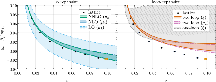
Figure 2: The renormalization-scale invariant quantity $y_{\text{c}}-\beta_{y}\log\mu_{3}$, where $y_{\text{c}}$ is the critical mass, $\mu_{3}$ is the renormalisation scale, and $\beta_{y}$ is the beta function for $y$. Theoretical uncertainties for lattice data are shown as (barely visible) error bars, while those for the perturbative calculations are shown as coloured bands. The latter are estimated either by varying the renormalization scale over $\mu_{3}/(2m_{A})\in[1/\sqrt{10},\sqrt{10}]$, or by varying the $R_{\xi}$ gauge parameter over $\xi\in[0,5]$. The hashed region shown on the right reflects the presence of a third unphysical phase in this approximation. The orange data point shows the location of the endpoint of the line of first-order phase transitions, as determined on the lattice.

Note the simplicity of using strict-perturbation theory as compared to a numerical approach: there is no need to numerically minimize (the real parts of) complicated potentials since everything is expressed in terms of the LO vev and critical mass.

Let us now turn to the latent heat, which determines the strength of a first-order phase transition. It is given by the temperature derivative of $\Delta V$. This can be written in terms of derivatives with respect to the 3d effective parameters $x$, $y$ and $g_{3}^{3}$, using the chain rule of differentiation Farakos et al. (1995). Dependence on the derivative with respect to $g_{3}^{3}$ cancels at the critical temperature Kajantie et al. (1996b). This leads us to calculate the following scalar condensates,

$$\Delta\braket{\Phi^{\dagger}\Phi} \equiv\frac{\partial}{\partial y}\Delta V, \Delta\braket{(\Phi^{\dagger}\Phi)^{2}} \equiv\frac{\partial}{\partial x}\Delta V,$$ (14)

which determine the contribution to the latent heat from the infrared EFT scale.

IV Results

Results at LO follow from the LO effective potential given in equation (6): the sum of tree-level and the one-loop term in figure 1(a). The minima can be found analytically, which yields simple expressions for thermodynamic observables.

NLO corrections arise from two-loop diagrams with loop momenta of order the vector boson mass. These diagrams, shown in figure 1b, appear through integrating out the heavy vectors for the EFT of the light scalars. Contributions to these diagrams from smaller loop momenta are subdominant, so scalar masses can be set to zero within loop integrals. The total NLO contribution to the effective potential is

$$V_{\text{NLO}}=\frac{\phi^{2}}{(4\pi)^{2}}\left(-\frac{51}{32}\log\frac{|\phi|}{\mu_{3}}-\frac{63}{32}\log\frac{3}{2}+\frac{33}{64}\right),$$ (15)

where $\mu_{3}$ is the 3d renormalization scale Farakos et al. (1994).

The NNLO potential consists of one-loop diagrams within the light scalar EFT. Expanded strictly in $x$, this is equivalent to the diagrams in figure 1c. These diagrams give

$$V_{\text{NNLO}}=-\frac{1}{12\pi}\left[\left(m_{H}^{2}(\phi)\right)^{3/2}+3\left(m_{G}^{2}(\phi)\right)^{3/2}\right].$$ (16)

The resummation of vector petals follows from equation (8).

With the effective potential in hand, we can calculate desired observables. Following the previous section we find

$$y_{\text{c}} =\frac{1-\frac{51}{2}x\log\tilde{\mu_{3}}-2\sqrt{2}x^{3/2}}{2(8\pi)^{2}x},$$ (17)

$$\Delta\braket{\Phi^{\dagger}\Phi}_{\text{c}} =\frac{1+\frac{51}{2}x+13\sqrt{2}x^{3/2}}{2(8\pi x)^{2}},$$ (18)

$$\Delta\braket{\left(\Phi^{\dagger}\Phi\right)^{2}}_{\text{c}} =\frac{1+51x+14\sqrt{2}x^{3/2}}{4(8\pi x)^{4}}.$$ (19)

where $\tilde{\mu}_{3}\equiv e^{-\tfrac{11}{34}+\tfrac{42}{34}\log\tfrac{3}{2}}(8\pi x\mu_{3})\approx 1.19(8\pi x\mu_{3})$. These expressions are accurate up to $O(x^{2})$ in the numerators.

Some information on the convergence of the perturbative expansion can be gleaned by comparing the magnitudes of successive terms. One finds that NLO terms in equations (17)-(19) can dominate over LO for $x\gtrsim 0.03$, choosing a renormalization scale $\mu_{3}\sim 1/(8\pi x)$. However, in each case the NNLO term remains smaller until significantly larger $x$. This suggests that the NLO term is anomalously large, and the perturbative expansion may be reliable at somewhat larger values of $x$, as indeed we find in our comparison to lattice data.

The explicit logarithm of the renormalization scale in equation (17) matches the implicit running of $y$, to ensure that $y-y_{\text{c}}$ is renormalization scale invariant at this order; for the beta functions see Refs. Farakos et al. (1994); Gould et al. (2022). By contrast, the absence of logarithms in the scalar condensates reflects the renormalization group invariance of these physical quantities. While the effective potential is $\mu_{3}$ dependent at NLO, this dependence cancels exactly in the observable quantity $\Delta V$.

The $x$-expansion is gauge-invariant and renormalization scale invariant order-by-order. However, residual renormalization scale dependence can be useful to estimate theoretical uncertainties. For $y_{\text{c}}$, this can be carried out by including the exact renormalization group running, rather than truncating at the order of $x$ calculated. Doing so includes running from terms suppressed by higher powers of $x$ than we have calculated, which therefore do not cancel. By contrast, the scalar condensates are simply renormalization group invariant, both exactly and order-by-order, so there is no way to introduce renormalization group running. This is nevertheless a desirable feature of the $x$-expansion, as it gives unambiguous predictions at each order.

Figures 2 and 3 compare perturbative and lattice results, the latter taken from Refs. Kajantie et al. (1996b); Gurtler et al. (1997); Rummukainen et al. (1998); Laine and Rummukainen (1999); Gould et al. (2022). The $x$-expansion for $y_{\text{c}}$ agrees well with the lattice over the entire range of $x$ for which there is a first-order phase transition, and the renormalization scale dependence gives a good estimate of the disagreement. By choosing $\mu_{3}\sim 2m_{A}$, one avoids large logarithms. There is a significant improvement from LO to NLO, and while the NNLO correction is small, it does shift towards the lattice data. Figure 3 shows similarly good agreement for the scalar condensates, though in this case the renormalization scale invariance of the $x$-expansion means there are no uncertainty bands. For the quadratic condensate, the NNLO correction improves agreement with the lattice only for $x\lesssim 0.05$, suggesting that above this higher-order terms become important. The quartic condensate shows the largest discrepancies between the $x$-expansion and the lattice data, which is consistent with the larger expansion coefficients for this quantity.

For comparison, in figure 2 we also show predictions based on a different perturbative approach: numerically minimising the real part of the one-loop and two-loop effective potentials. This approach is commonly taken in the literature but, for radiatively-induced transitions, it is not an expansion in any small parameter, because loop-level contributions are of the same size as tree-level terms. Further, directly minimising the real part of the effective potential cancels neither gauge nor renormalization-scale dependence at each order. The large uncertainty at one-loop order in this approach is due to the presence of a third unphysical phase for $R_{\xi}$ gauge parameters $\xi\gtrsim 3$. Predictions for all the condensates in this approach gain an imaginary part for $y<0$.

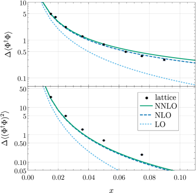
Figure 3: The jumps in the scalar condensates as functions of $x$, computed in the $x$-expansion and on the lattice. Both condensates are manifestly gauge and renormalization-scale invariant.

V Conclusions

We find that strong first-order phase transitions can be described rather well by perturbation theory. We have developed an EFT approach to transitions with radiatively-generated barriers, and performed calculations up to NNLO. The main results of this paper are presented in equations (17)–(19) and in Figs. 2 and 3. For the SU(2) Higgs theory, we find good numerical agreement between our perturbative expansion, in powers of $x$, and existing lattice data.

The existence of the $x$-expansion was recognised in the late 90s Kajantie et al. (1997b, 1998); Moore and Rummukainen (2001), yet in the two intervening decades it has not been used once, to our knowledge. In this paper, we revive this forgotten idea, and make the first major advancement since its introduction. We elucidate the underlying structure of the $x$-expansion, and develop the tools necessary to extend the expansion to higher orders. This allows us to push calculations to NNLO for the first time —the lowest order at which resummations are necessary within 3d.

The $x$-expansion is theoretically well-behaved in the sense that it does not suffer from IR-divergences or gauge-dependence, and renormalization scale-dependence cancels order-by-order. In addition, contrary to previous calculations Arnold (1994); Arnold and Espinosa (1993), our results indicate good convergence. Though the results are consistent with lattice calculations, and better behaved than those of other methods, the expansion can still be improved. As we have seen, going to NLO is very important to get a reasonably accurate prediction. The next improvement to NNLO is numerically smaller, but improves agreement with the lattice results for $x\lesssim 0.05$.

Our results can be contrasted with QCD, where there is a sizeable mismatch between perturbative and lattice calculations of the free energy density Zhai and Kastening (1995); Braaten and Nieto (1996). This can be partially ascribed to the absence of a Higgs phase in QCD, within which perturbation theory is comparatively well under control, but also to the relatively large magnitude of the QCD gauge coupling, and its slow (logarithmic) approach to asymptotic freedom.

The $x$-expansion, like all other perturbative approaches to non-Abelian gauge fields at high temperature, breaks down at finite order due to the Linde Problem Linde (1980). For the free energy density, nonperturbative infrared physics contributes first at $O(g^{6}T^{4})$. For the quantities studied here, this means that starting at N⁵LO, which is suppressed by $O(x^{3})$, the $x$-expansion is fundamentally nonperturbative. However, the Linde Problem cannot modify the leading five coefficients of the asymptotic expansion, and hence it does not stop the $x$-expansion performing well for small enough $x$.

Future studies can utilize the approach taken here for other models. The remaining higher-order terms in the expansion should also be calculated: N³LO and N⁴LO, respectively $O(x^{2})$ and $O(x^{5/2})$. Doing so requires calculation of three-loop diagrams. These two terms are the highest order terms that are completely calculable in perturbation theory and therefore give the final word on how well the expansion actually works.

Finally, given the importance of a strict expansion for equilibrium quantities, we expect similar behaviour for near-equilibrium ones, like the bubble-nucleation rate Ekstedt (2022). As such our results are an important stepping-stone for accurate predictions of gravitational waves.