Double Flip Move for Ising Models with Mixed Boundary Conditions

Abstract.

This note introduces the double flip move for accelerating the Swendsen-Wang algorithm for Ising models with mixed boundary conditions below the critical temperature. The double flip move consists of a geometric flip of the spin lattice followed by a spin value flip. Both the symmetric and approximately symmetric models are considered. We prove the detailed balance of the double flip move and demonstrate its empirical efficiency in mixing.

1. Introduction

This note is concerned with the Monte Carlo sampling of Ising models with mixed boundary conditions. Consider a graph $G=(V,E)$ with the vertex set $V$ and the edge set $E$. Assume that $V=I\cup B$, where $I$ is the subset of interior vertices and $B$ the subset of boundary vertices. Throughout the note, we use $i,j$ to denote the vertices in $I$ and $b$ for the vertices in $B$. $E$ is the set of edges, where $ij\in E$ denotes an interior edge while $ib\in E$ denotes an edge between an interior vertex $i$ and a boundary vertex $b$. The boundary condition is specified by $f=(f_{b})_{b\in B}$. The Ising model with the boundary condition $f$ is the following probability distribution $p_{\mathrm{V}}(\cdot)$ over the configurations $s=(s_{i})_{i\in I}$ of the interior vertex set $I$:

(1) $$p_{\mathrm{V}}(s)\sim\exp\left(\beta\sum_{ij\in E}s_{i}s_{j}+\beta\sum_{ib\in E}s_{i}f_{b}\right).$$

One key feature of these models is that below the critical temperature the Gibbs distribution exhibits on the macroscopic scale different profiles dictated by the boundary condition. Figure 1 showcases two such examples, where black denotes $+1$ and white denotes $-1$. In Figure 1(a), the square Ising lattice has the $+1$ condition on the two vertical sides but the $-1$ condition on the two horizontal sides. There are two dominant profiles: one contains a large $-1$ cluster linking two horizontal sides and the other contains a large $+1$ cluster linking two vertical sides. In Figure 1(b), the Ising lattice supported on a disk has the $+1$ condition on two disjoint arcs and the $-1$ condition on the other two. The two dominant profiles are shown in Figure 1(b). Notice that in each example, due to the symmetry or approximate symmetry of the Ising lattice and the boundary condition, the two dominant profiles have comparable probabilities. Therefore, any effective sampling algorithm is required to visit both profiles frequently.

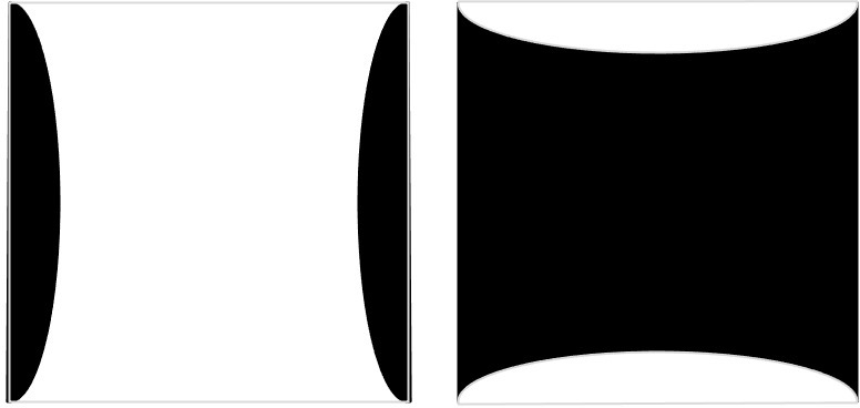
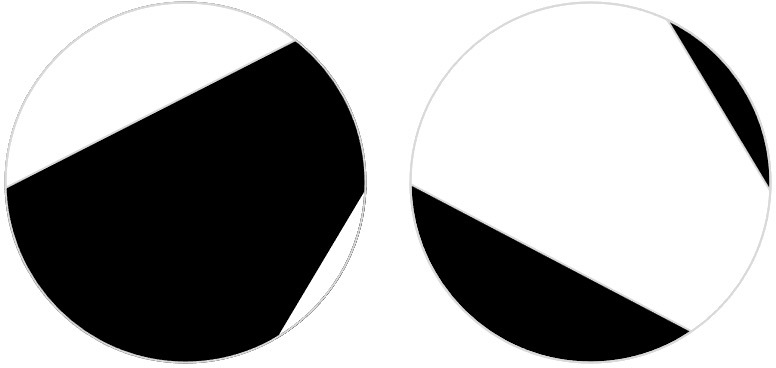
(a)	(b)

Figure 1. Ising models with mixed boundary condition. (a) a square lattice and (b) a lattice support on a disk. In each example, the model exhibits two dominant profiles on the macroscopic scale.

One of the most well-known methods for sampling Ising models is the Swendsen-Wang algorithm [swendsen1987nonuniversal], which iterates between the following two substeps in each iteration

1. Given the current spin configuration, generate an edge configuration according the temperature (see Section 2 for details).

2. To each connected component of the edge configuration, assign all $+1$ or all $-1$ to its spins with equal probability. This results in a new spin configuration.

For many boundary conditions including the free boundary condition, the Swendsen-Wang algorithm exhibits rapid mixing for all temperatures. However, for the mixed boundary conditions shown in Figure 1, the Swendsen-Wang algorithm experiences slow convergence under the critical temperatures, i.e., $T<T_{c}$ or equivalently $\beta>\beta_{c}$ in terms of the inverse temperature. The reason is that, for such a boundary condition, the energy barrier between the two dominant profiles is much higher than the energy of these profiles. In other words, the Swendsen-Wang algorithm needs to break a macroscopic number of edges between aligned adjacent spins in order to transition from one dominant profile to the other. However, breaking so many edges simultaneously is an event with exponentially small probability.

In this note, we introduce the double flip move that introduces direct transitions between these dominant profiles. When combined with the Swendsen-Wang algorithm, it accelerates the mixing of these Ising model under the critical temperature significantly.

When the Ising model exhibits an exact symmetry (typically a reflection that negates the mixed boundary condition), the double flip move consists of

1. A geometric flip of the spin lattice along a symmetry line, followed by

2. A spin-value flip at the interior vertices of the Ising model.

The key observation is that these two flips together preserves the alignment between the adjacent spins, hence introducing a successful Monte Carlo move. When the Ising model exhibits only an approximate symmetry, the double flip move consists of

1. A geometric flip of the spin lattice along a symmetry line,

2. A matching step that snaps the flipped copy of the interior vertices to the original copy of the interior vertices, and

3. A spin-value flip at the interior vertices of the Ising model.

In both the exact and the approximate symmetry case, we prove the detailed balance of the double flip move and demonstrate its efficiency when combined with the Swendsen-Wang algorithm.

Related works. In [alexander2001spectral, alexander2001spectralB], Alexander and Yoshida studied the spectral gap of the 2D Ising models with mixed boundary conditions. More recently, in [gheissari2018effect], Gheissari and Lubetzky studied the effect of the boundary condition for the 2D Potts models at the critical temperature. In [chatterjee2020speeding], Chatterjee and Diaconis showed that most of the deterministic jumps can accelerate the Markov chain mixing when the equilibrium distribution is uniform.

Contents. The rest of the note is organized as follows. Section 2 reviews the Swendsen-Wang algorithm for the Ising models with boundary condition. Section 3 describes the double flip move for models with exact symmetry and Section 4 extends it to models with approximate symmetry. Section 5 discusses some future directions.

2. Swendsen-Wang algorithm

In this section, we briefly review the Swendsen-Wang algorithm, which is a Markov Chain Monte Carlo method for sampling $p_{\mathrm{V}}(\cdot)$. The description here is adapted to the setting with boundary condition. In each iteration, it generates a new configuration $t$ from the current configuration $s$ as follows:

1. Generate an edge configuration $w=(w_{ij})_{ij\in E}$. If the spin values $s_{i}$ and $s_{j}$ are different, set $w_{ij}=0$. If $s_{i}$ and $s_{j}$ are the same, $w_{ij}$ is sampled from the Bernoulli distribution $\mathrm{Ber}(1-e^{-2\beta})$, i.e., equal to 1 with probability $1-e^{-2\beta}$ and 0 with probability $e^{-2\beta}$.

2. Regards all edges $ij\in E$ with $w_{ij}=1$ and $ib\in E$ with $w_{ib}=1$ as linked. Compute the connected components. For each connected component $\gamma$, if $\gamma$ contains a boundary vertex, set $(t_{i})_{i\in\gamma}$ to the spin of the boundary vertex. If not, set all the spins $(t_{i})_{i\in\gamma}$ to all $-1$ or all $+1$ with equal probability.

The following two related probability distributions are important for analyzing the Swendsen-Wang algorithm [edwards1988generalization]. The first one is the joint vertex-edge distribution

(2) $$p_{\mathrm{VE}}(s,w)\sim \prod_{ij\in E}\left((1-e^{-2\beta})\delta_{s_{i}=s_{j}}\delta_{w_{ij}=1}+e^{-2\beta}\delta_{w_{ij}=0}\right)\cdot$$

$$\prod_{ib\in E}\left((1-e^{-2\beta})\delta_{s_{i}=f_{b}}\delta_{w_{ib}=1}+e^{-2\beta}\delta_{w_{ib}=0}\right).$$

The second one is the edge distribution

(3) $$p_{\mathrm{E}}(w)\sim\prod_{w_{ij}=1}(1-e^{-2\beta})\prod_{w_{ij}=0}e^{-2\beta}\cdot\prod_{w_{ib}=1}(1-e^{-2\beta})\prod_{w_{ib}=0}e^{-2\beta}\cdot 2^{|\mathcal{C}_{w}|},$$

where $\mathcal{C}_{w}$ is set of connected components of $w$ that contain only the interior vertices.

Summing $p_{\mathrm{VE}}(s,w)$ over $s$ or $w$ gives [edwards1988generalization]

(4) $$\sum_{s}p_{\mathrm{VE}}(s,w)=p_{\mathrm{E}}(w),\quad\sum_{w}p_{\mathrm{VE}}(s,w)=p_{\mathrm{V}}(s).$$

A direct consequence of (4) is that the Swendsen-Wang algorithm can be viewed as a data augmentation method [liu2001monte], where the first substep samples the edge configuration $w$ conditioned on the spin configuration $s$ and the second substep samples a new spin configuration $t$ conditioned on the edge configuration $w$.

This relationship (4) also shows that Swendsen-Wang algorithm satisfies the detailed balance, i.e.,

$$p_{\mathrm{V}}(s)P_{\mathrm{SW}}(s,t)=p_{\mathrm{V}}(t)P_{\mathrm{SW}}(t,s),$$

where $P_{\mathrm{SW}}$ is for the Swendsen-Wang transition matrix. To see this, note that $P_{\mathrm{SW}}(s,t)=\sum_{w}P_{w}(s,t)$ and $P_{\mathrm{SW}}(t,s)=\sum_{w}P_{w}(t,s)$, where the sum in $w$ is taken over all compatible edge configurations $w$ and $P_{w}(s,t)$ is the transition probability from $s$ to $t$ via the edge configuration $w$. Therefore, it is sufficient to show

$$p_{\mathrm{V}}(s)P_{w}(s,t)=p_{\mathrm{V}}(t)P_{w}(t,s)$$

for any compatible edge configuration $w$. Since the transitions from the edge configuration $w$ to the spin configurations $s$ and $t$ are the same, it reduces to showing

$$p_{\mathrm{V}}(s)P(s,w)=p_{\mathrm{V}}(t)P(t,w),$$

where $P(s,w)$ is the probability of obtaining the edge configuration $w$ from $s$ and similarly for $P(t,w)$. In fact $p_{\mathrm{V}}(s)P(s,w)$ is independent of the spin configuration $s$ by the following argument. First, if an edge $ij\in E$ has configuration $w_{ij}=1$, then $s_{i}=s_{j}$. Second, if $ij\in E$ has configuration $w_{ij}=0$, then $s_{i}$ and $s_{j}$ can either be the same or different. In the former case, the contribution to $p_{\mathrm{V}}(s)P(s,w)$ from $ij$ is $e^{2\beta}\cdot e^{-2\beta}=1$ up to a normalization constant. In the latter case, the contribution is $1\cdot 1=1$ up to the same normalization constant. The same argument applies to the edges $ib\in E$ and therefore $p_{\mathrm{V}}(s)P(s,w)$ is independent of $s$.

The Swendsen-Wang algorithm unfortunately does not encourage transitions between the dominant profiles shown in Figure 1. For these mixed boundary condition, such a transition requires breaking a macroscopic number of edges between aligned adjacent spins, which has an exponentially small probability. This is the motivation for introducing the double flip move.

3. Double flip for symmetric models

The double flip move is designed to introduce explicit transitions between the different profiles as shown Figure 1. This section assumes that the Ising model enjoys an explicit graph involution, i.e., there exists a map $m:V\rightarrow V$ such that

• $m$ maps $I$ to $I$ and $B$ to $B$, respectively, and $m^{2}=\mathrm{id}$,

• $ij\in E$ iff $m(i)\sim m(j)\in E$, and $ib\in E$ iff $m(i)m(b)\in E$,

• $f_{m(b)}=-f_{b}$.

For example, in Figure 2(a) $m$ is the reflection along one of the diagonals of the square, while in Figure 3(a) $m$ is the reflection along either the $x$ axis or the $y$ axis.

In the double flip move, the first flip implements the map $m$ to the interior vertices in $I$. After that, the second flip negates the spin of the mapped interior vertices. More specifically, the resulting new spin configuration $t$ is defined by

(5) $$t_{m(i)}=-s_{i},\quad\forall i\in I.$$

Since $m^{2}=\mathrm{id}$, we also have $t_{i}=-s_{m(i)}$ for any $i\in I$.

Theorem 1.

The double flip move satisfies the detailed balance.

Proof.

To show the detailed balance, one needs to prove that, for any two spin configurations $s$ and $t$,

$$p_{\mathrm{V}}(s)P_{\mathrm{DF}}(s,t)=p_{\mathrm{V}}(t)P_{\mathrm{DF}}(t,s),$$

where $P_{\mathrm{DF}}$ is the double flip move transition matrix. From the definition of the double flip move, the transition probabilities $P(s,t)$ and $P(t,s)$ equal to one if $s$ and $t$ satisfy (5) and zero otherwise. Hence it is sufficient to show $p_{\mathrm{V}}(s)=p_{\mathrm{V}}(t)$ when (5) holds.

For each $ij\in E$,

$$t_{i}t_{j}=(-1)^{2}s_{m(i)}s_{m(j)}=s_{m(i)}s_{m(j)}.$$

Taking the sum over all interior edges gives

$$\sum_{ij\in E}t_{i}t_{j}=\sum_{ij\in E}s_{m(i)}s_{m(j)}=\sum_{ij\in E}s_{i}s_{j}.$$

For each $ib\in E$,

$$t_{i}f_{b}=(-1)^{2}s_{m(i)}f_{m(b)}=s_{m(i)}f_{m(b)}.$$

Taking the sum over all interior edges results in

$$\sum_{ib\in E}t_{i}f_{b}=\sum_{ib\in E}s_{m(i)}f_{m(b)}=\sum_{ib\in E}s_{i}f_{b}.$$

Together, $\sum_{ij\in E}t_{i}t_{j}+\sum_{ib\in E}t_{i}f_{b}=\sum_{ij\in E}s_{i}s_{j}+\sum_{ib\in E}s_{i}f_{b}$, i.e., $p_{\mathrm{V}}(s)=p_{\mathrm{V}}(t)$. ∎

We can now combine the double flip move with the Swendsen-Wang move. For a constant $\eta\in(0,1)$, each iteration of the combined algorithm performs the double flip move with probability $\eta$ and the Swendsen-Wang move with probability $1-\eta$.

1. Choose $u$ from $\mathrm{Ber}(\eta)$, i.e., equal to 1 with probability $\eta$.

2. If $u$ is 1, perform the double flip move, else perform the Swendsen-Wang move.

Theorem 2.

The Swendsen-Wang algorithm with double flip satisfies the detailed balance.

Proof.

The combined transition matrix is

$$P_{\mathrm{SWDF}}=\eta P_{\mathrm{DF}}+(1-\eta)P_{\mathrm{SW}}.$$

Section 2 shows that the Swendsen-Wang algorithm satisfies the detailed balance, i.e.,

$$p_{\mathrm{V}}(s)P_{\mathrm{SW}}(s,t)=p_{\mathrm{V}}(t)P_{\mathrm{SW}}(t,s).$$

The double flip move satisfies the detailed balance as shown above,

$$p_{\mathrm{V}}(s)P_{\mathrm{DF}}(s,t)=p_{\mathrm{V}}(t)P_{\mathrm{DF}}(t,s).$$

A linear combination of these two statements give

$$p_{\mathrm{V}}(s)P_{\mathrm{SWDF}}(s,t)=p_{\mathrm{V}}(t)P_{\mathrm{SWDF}}(t,s)$$

and this finishes the proof. ∎

Below we compare the performance of the Swendsen-Wang algorithm (SW) and Swendsen-Wang with double flip (SWDF) using two examples.

Example 1.

The Ising model is a square lattice. The mixed boundary condition is $+1$ at the two vertical sides and $-1$ at the two horizontal sides. The graph involution $m:V\rightarrow V$ is given by the diagonal reflection. Figure 2(a) shows the model at size $n_{1}=n_{2}=20$.

The experiments are performed for the problem size $n_{1}=n_{2}=100$ at the inverse temperature $\beta=0.5$. We start from the all $-1$ configuration and carry out $10000$ iterations for both SW and SWDF. For SWDF, we set the parameter $\eta=1/100$. Figure 2(b) and (c) plot the average spin value

$$\frac{1}{|I|}\sum_{i\in I}s_{i}$$

of these two algorithms, respectively. Figure 2(b) shows that SW fails to introduce transitions between the $-1$ and the $+1$ dominant profiles, since the average spin is always below $0$. On the other hand, Figure 2(c) demonstrates that SWDF explores both profiles with $100$ transitions in between.

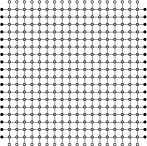
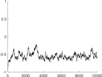
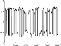
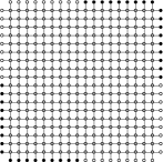
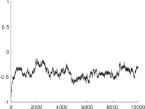
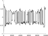
(a)	(b)	(c)

Figure 2. (a) The lattice along with the mixed boundary condition (black for $+1$ and white for $-1$). (b) The average spin value of the Swendsen-Wang algorithm. (c) The average spin value of the Swendsen-Wang algorithm with double flip.

Example 2.

The Ising lattice is still a square. The mixed boundary condition is $+1$ in the first and third quadrants but $-1$ in the second and fourth quadrants. The graph involution $m:V\rightarrow V$ is given by the reflection along either the $x$ or the $y$ axis. Figure 3(a) shows the problem at size $n_{1}=n_{2}=20$.

Similar to the previous example, the experiments are performed for the problem size $n_{1}=n_{2}=100$ at the inverse temperature $\beta=0.5$. We start from the all $-1$ configuration and carry out $10000$ iterations for both SW and SWDF. The $\eta$ parameter of SWDF is $\eta=1/100$. Figure 3(b) shows that SW fails to introduce transitions between the $-1$ dominant and the $+1$ dominant profiles, while Figure 3(c) demonstrates that SWDF explores both profiles with $100$ transitions in between.

(a)	(b)	(c)

Figure 3. (a) The lattice along with the mixed boundary condition (black for $+1$ and white for $-1$). (b) The average spin value of the Swendsen-Wang algorithm. (c) The average spin value of the Swendsen-Wang algorithm with double flip.

4. Double flip for approximately symmetric models

The algorithm in Section 3 is efficient but depends on exact symmetries. However, many Ising models without exact symmetries also exhibit multiple dominant profiles such as in Figure 1. This section extends the double flip move to models with approximate symmetry.

To take a more geometric viewpoint, assume that the Ising model is embedded in a domain $\Omega\subset\mathbb{R}^{2}$ with the boundary denoted by $\partial\Omega$.

• For each $i\in I$, $x_{i}$ is in the interior of $\Omega$. For each $b\in B$, $x_{b}$ is in $\partial\Omega$.

• The edges $ij$ or $ib$ in the edge set $E$ are segments between geometrically nearby vertices.

• $\partial\Omega=\partial\Omega_{+}\cup\partial\Omega_{-}$. If $x_{b}\in\partial\Omega_{+}$, then $f_{b}=1$. If $x_{b}\in\partial\Omega_{-}$, then $f_{b}=-1$.

• Assume that there is a continuous involution $\mu:\bar{\Omega}\rightarrow\bar{\Omega}$ such that $\mu^{2}=\mathrm{id}$ and $\mu(\partial\Omega_{+})=\partial\Omega_{-}$.

As $\mu$ is only defined as an involution of $\Omega$, in general $\{\mu(x_{i})\}_{i\in I}\not=\{x_{i}\}_{j\in I}$ and therefore $\mu$ does not directly introduce an involution on the set $I$ of interior vertices. To fix this, we introduce a discrete involution $m:I\rightarrow I$ such that

(6) $$x_{m(i)}\approx\mu(x_{i}).$$

We shall discuss below how to construct $m$ based on $\mu$. For now, assuming the existence of $m$, one can define a Metropolized double flip move for approximately symmetric models.

1. Define a spin configuration $t$ via $t_{i}=-s_{m(i)}$.

2. Evaluate $c=\min(1,p_{\mathrm{V}}(t)/p_{\mathrm{V}}(s))$.

3. Sample $u\in[0,1]$ uniformly. If $u\leq c$, set $t$ to be the new spin configuration. Otherwise, keep $s$ as the spin configuration.

Since $m$ is an involution and this is a Metropolized move, the following statement holds.

Theorem 3.

The Metropolized double flip move satisfies the detailed balance.

It can also be combined with the Swendsen-Wang move in the same way as described in Section 3.

Theorem 4.

The Swendsen-Wang algorithm with Metropolized double flip satisfies the detailed balance.

The efficiency of this algorithm depends on the criteria of $p_{\mathrm{V}}(t)/p_{\mathrm{V}}(s)$ neither too small or too large. This is in fact promoted by the condition (6), since $ij\in E$ implies

$$x_{m(i)}\approx\mu(x_{i})\approx\mu(x_{j})\approx x_{m(j)},$$

where the second step uses the continuity of the domain involution $\mu$. Therefore, when $ij\in E$, $m(i)m(j)$ is also likely to be an edge of $E$ with

$$s_{i}s_{j}=(-1)^{2}s_{i}s_{j}=t_{m(i)}t_{m(j)}.$$

If this holds for most pairs $ij\in E$ and $ib\in E$, we have $p_{\mathrm{V}}(t)/p_{\mathrm{V}}(s)$ under control.

The remaining question is how to construct $m:I\rightarrow I$ so that (6) holds and $m^{2}=\mathrm{id}$. One possibility is to formulate this as a matching problem between the geometrically flipped vertices $\{\mu(x_{i})\}_{i\in I}$ and the original vertices $\{x_{j}\}_{j\in I}$, with a cost defined using the $\ell_{2}$ or $\ell_{\infty}$ distance. Equivalently, this is an optimal transport problem between the two distributions

$$\sum_{i\in I}\delta_{\mu(x_{i})}(\cdot)\quad\text{and}\quad\sum_{j\in I}\delta_{x_{j}}(\cdot).$$

Once the matching (or the transport map) is available, we define $m(i)=j$ if $\mu(x_{i})$ is matched with $x_{j}$. However, this approach has two technical difficulties.

• The computation cost of the matching or optimal transport algorithm [kuhn1955hungarian, peyre2019computational] can be relatively high.

• The involution condition $m^{2}=\mathrm{id}$ is not guaranteed.

In the implementation, we adopt the following heuristic procedure. Assume without loss of generality that the domain $\Omega$ is centered at the origin.

1. Order the interior vertices $\{x_{j}\}_{j\in I}$ based on their distances to the origin in the decreasing order. The distance is typically chosen to be the $\ell_{\infty}$ norm or the $\ell_{2}$ norm.

2. Mark all vertices $j\in I$ as unpaired.

3. Scan the interior vertices in this ordered list. For each $x_{j}$, if $j$ is already paired, then skip. If not, find the unpaired $i$ such that $\mu(x_{i})$ is closet to $x_{j}$, pair $i$ and $j$

   $$m(i):=j,\quad m(j):=i,$$

   and mark both $i$ and $j$ as paired.

The heuristic is that, by following the order of decreasing distance to the origin, the unpaired vertices are forced to cluster near the center of the domain, thus reducing the overall transport cost.

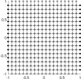
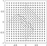
(a)	(b)
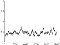
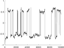
(c)	(d)

Figure 4. (a) The rectangular lattice along with the mixed boundary condition (black for $+1$ and white for $-1$). (b) The transport map from $\{\mu(x_{i})\}_{i\in I}$ (marked with $+$) to $\{x_{j}\}_{j\in I}$ (marked with $\circ$). (c) The average spin value of the Swendsen-Wang algorithm. (d) The average spin value of the Swendsen-Wang algorithm with double flip.

Below we compare the performance of the Swendsen-Wang algorithm (SW) and Swendsen-Wang with Metropolized double flip (SWDF) using three examples.

Example 3.

The Ising model is a rectangular lattice where the number of rows and columns are different, as shown in Figure 4. The mixed boundary condition is $+1$ at the two vertical sides and $-1$ at the two horizontal sides. The diagonal reflection is no longer an exact symmetry. Figure 4(a) shows the system with size $20\times 19$. Figure 4(b) plots the transport map between $\{\mu(x_{i})\}_{i\in I}$ (marked with $+$) to $\{x_{j}\}_{j\in I}$ (marked with $\circ$). As shown, the transport map is quite local, demonstrating the efficiency of the heuristic matching procedure.

The experiments are performed for the problem size $100\times 99$ at the inverse temperature $\beta=0.5$. We start from the all $-1$ configuration and carry out $10000$ iterations for both SW and SWDF. The $\eta$ parameter of SWDF is $\eta=1/3$. Figure 4(c) shows that SW fails to introduce transitions between the $-1$ dominant and the $+1$ dominant profiles, while Figure 4(d) demonstrates that SWDF explores both profiles with $41$ transitions out of about $3000$ trials.

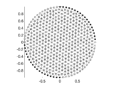
(a)	(b)
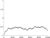
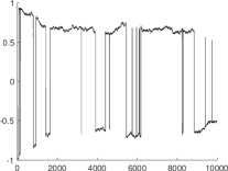
(c)	(d)

Figure 5. (a) The lattice along with the mixed boundary condition (black for $+1$ and white for $-1$). (b) The transport map from $\{\mu(x_{i})\}_{i\in I}$ (marked with $+$) to $\{x_{j}\}_{j\in I}$ (marked with $\circ$). (c) The average spin value of the Swendsen-Wang algorithm. (d) The average spin value of the Swendsen-Wang algorithm with double flip.

Example 4.

The Ising model is a random quasi-uniform triangular lattice supported on the unit disk, as shown in Figure 5. The mixed boundary condition is equal to $+1$ in the first and third quadrants but $-1$ in the second and fourth quadrants. The problem does not have strict rotation and reflection symmetry due to the random triangulation. Figure 5(a) shows the triangulation with mesh size $h=0.1$. Figure 5(b) gives the transport map between $\{\mu(x_{i})\}_{i\in I}$ (marked with $+$) to $\{x_{j}\}_{j\in I}$ (marked with $\circ$), which is quite local.

The experiments are performed with a finer triangulation with mesh size $h=0.05$ at the inverse temperature $\beta=0.5$. We start from the all $-1$ configuration and carry out $10000$ iterations for both SW and SWDF. The $\eta$ parameter of SWDF is $\eta=1/3$. Figure 5(c) shows that SW fails to introduce transitions between the $-1$ dominant and the $+1$ dominant profiles, while Figure 5(d) demonstrates that SWDF explores both profiles with $48$ transitions out of about $3000$ trials.

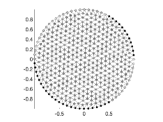
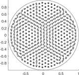
(a)	(b)
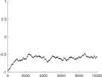
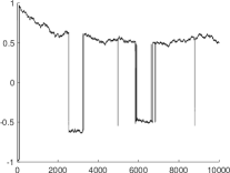
(c)	(d)

Figure 6. (a) The lattice along with the mixed boundary condition (black for $+1$ and white for $-1$). (b) The transport map from $\{\mu(x_{i})\}_{i\in I}$ (marked with $+$) to $\{x_{j}\}_{j\in I}$ (marked with $\circ$). (c) The average spin value of the Swendsen-Wang algorithm. (d) The average spin value of the Swendsen-Wang algorithm with double flip.

Example 5.

The Ising model is again a random quasi-uniform triangular lattice supported on the unit disk. The mixed boundary condition is equal to $+1$ on the two arcs with angle in $[0,\pi/3]$ and $[\pi,5\pi/3]$ but $-1$ on the remaining two arcs. Due to the random triangulation, the problem does not have strict rotation and reflection symmetry. Figure 6(a) shows the triangulation with mesh size $h=0.1$. Figure 6(b) plots the transport map between $\{\mu(x_{i})\}_{i\in I}$ (marked with $+$) to $\{x_{j}\}_{j\in I}$ (marked with $\circ$).

The experiments are performed with a finer triangulation with mesh size $h=0.05$ at the inverse temperature $\beta=0.5$. We start from the all $-1$ configuration and carry out $10000$ iterations for both SW and SWDF. The $\eta$ parameter of SWDF is $\eta=1/3$. Figure 6(c) shows that SW fails to introduce transitions between the $-1$ dominant and the $+1$ dominant profiles, while Figure 6(d) demonstrates that SWDF explores both profiles with $35$ transitions out of about $3000$ trials.

5. Discussions

This note introduces the double flip move for accelerating the Swendsen-Wang algorithm for Ising models with mixed boundary conditions. We consider both symmetric and approximately symmetric models. In both cases, we prove the detailed balance and demonstrated its efficiency in introducing explicit transitions between different dominant profiles.

There are many unanswered questions. Regarding the symmetric models, one question is to prove a polynomial mixing time for the examples in Section 3. Regarding the approximately symmetric models, there are more open questions.

• Is there a fast matching or optimal transport algorithm that ensures $m^{2}=\mathrm{id}$?

• Better heuristic procedures for constructing the matching between $\{\mu(x_{i})\}_{i\in I}$ and $\{x_{j}\}_{j\in I}$?

• Can we bound the acceptance ratio of the Metropolized double flip move under certain assumptions of the approximate symmetry?

• Proving a rapid mixing result for any approximately symmetric model in Section 4.

• The approximate matching is carried out for the interior vertices in this note. However, it can be carried out for the edges alternatively.