Search for the Gravitational-wave Background from Cosmic Strings with the Parkes Pulsar Timing Array Second Data Release
Abstract
We perform a direct search for an isotropic stochastic gravitational-wave background (SGWB) produced by cosmic strings in the Parkes Pulsar Timing Array second data release. We find no evidence for such an SGWB, and therefore place confidence level upper limits on the cosmic string tension, , as a function of the reconnection probability, , which can be less than 1 in the string-theory-inspired models. The upper bound on the cosmic string tension is for , which is about five orders of magnitude tighter than the bound derived from the null search of individual gravitational wave burst from cosmic string cusps in the PPTA DR2.
I Introduction
Over the past few years, the gravitational wave (GW) community witnessed the detection of a population of GW events Abbott et al. (2019, 2021a, 2021b, 2021c) with ground-based interferometers that are sensitive in frequencies from Hz to kHz. A pulsar timing array (PTA) Sazhin (1978); Detweiler (1979); Foster and Backer (1990) offers a unique opportunity of extending the GW observations to the very low frequencies from nHz to Hz, by regularly monitoring the time of arrivals (TOAs) of radio pulses from an array of highly stable millisecond pulsars in the Milky Way. There are three major PTA projects, namely the European PTA (EPTA) Kramer and Champion (2013), the North American Nanoherz Observatory for GWs (NANOGrav) McLaughlin (2013), and the Parkes PTA (PPTA) Manchester et al. (2013). These PTA projects have been monitoring the TOAs from dozens of pulsars with a weekly to monthly cadence for more than a decade. These PTAs along with the Indian PTA (InPTA) Joshi et al. (2018), the Chinese PTA (CPTA) Lee (2016) and the MeerKAT interferometer Bailes et al. (2020), support the International PTA (IPTA) Hobbs et al. (2010); Manchester (2013). Potential GW sources in the PTA frequency band include a variety of physical phenomena such as supermassive black hole binaries (SMBHBs) Jaffe and Backer (2003); Sesana et al. (2008, 2009), scalar-induced GWs Saito and Yokoyama (2009); Yuan et al. (2019a, b); Chen et al. (2020); Yuan et al. (2019c); Chen et al. (2022), first-order phase transition Witten (1984); Hogan (1986), and cosmic strings Lentati et al. (2015); Blanco-Pillado et al. (2018); Arzoumanian et al. (2018a); Yonemaru et al. (2021).
Recently, the NANOGrav Arzoumanian et al. (2020a), PPTA Goncharov et al. (2021a), EPTA Chen et al. (2021a) and IPTA Antoniadis et al. (2022) successively reported strong evidence for a stochastic common-spectrum process modeled by a power-law spectrum in their latest data sets. However, there is no significant evidence for the tensor transverse spatial correlations, which are necessary to claim a detection of stochastic GW background (SGWB) predicted by general relativity. The origin of this spatially uncorrelated common-spectrum process (UCP) is still unknown. Further investigations indicate that the UCP can possibly come from various physical processes such as phase transitions Addazi et al. (2021); Ratzinger and Schwaller (2021); Bian et al. (2021); Li et al. (2021); Xue et al. (2021); Arzoumanian et al. (2021a), domain walls Bian et al. (2021); Wang (2022); Ferreira et al. (2022), cosmic strings Blasi et al. (2021); Ellis and Lewicki (2021); Bian et al. (2021); Wang (2022), or the non-tensorial polarization modes from alternative gravity theories Chen et al. (2021b); Arzoumanian et al. (2021b); Wu et al. (2022); Chen et al. (2021c).
Cosmic strings are linear topological defects that can either form in the early Universe from symmetry-breaking phase transitions at high energies Kibble (1976); Vilenkin (1981, 1985); Dvali and Vilenkin (2004) or be the fundamental strings of superstring theory (or one-dimensional D-branes) stretched out to astrophysical lengths Dvali and Vilenkin (2004); Copeland et al. (2004). After their formation, the intersection between cosmic strings can lead to reconnections and form loops, which will then decay due to relativistic oscillation and emit GWs. PTA observations may detect a cosmic string network either through GW bursts emitted at cusps or through the SGWB superposed by radiation from all loops existing through cosmic history. A null detection of the individual GW burst from cosmic strings in PPTA DR2 has been reported in Yonemaru et al. (2021), thus placing a upper limit on the cosmic string tension to be . In this work, we perform the first direct search for the SGWB produced from a network of cosmic strings in the PPTA DR2 data set. The remainder of this paper is organized as follows. In Sec. II, we review the SGWB energy spectrum produced by the cosmic strings. In Sec. III, we describe the data set and methodology used in our analyses. Finally, we summarize the results and give some discussion in Sec. IV.
II SGWB from cosmic strings
We now review the SGWB produced by cosmic strings following Blanco-Pillado and Olum (2017). A cosmic string network consists of both long (or “infinite”) strings that are longer than the horizon size and loops formed from smaller strings. When two cosmic strings meet one another, they can exchange partners with a reconnection probability , and form loops. Once loops are formed, they oscillate and decay through the emission of GWs Vilenkin (1981), shrinking in size. A cosmic string network grows along with the cosmic expansion and evolves toward the scaling regime in which all the fundamental properties of the system scale with the cosmic time. The scaling regime can be achieved through the formation and subsequent decay of loops. The GW spectrum created by a cosmic string network is exceptionally broadband, depending on the size of the loops created.
We describe the GW energy spectrum of cosmic strings in terms of the dimensionless tension, , and the reconnection probability, . Even though for classical strings, it can be less than 1 in the string-theory-inspired models. In this work, we adopt the convention that the speed of light . The dimensionless GW energy density parameter per logarithm frequency as the fraction of the critical energy density is Blanco-Pillado and Olum (2017)
| (1) |
where is cosmic time today, and is the GW energy density per unit frequency that can be computed by
| (2) |
with
| (3) |
Here, is the radiation power spectrum of each loop, and is the density of loops per unit volume per unit range of loop length existing at time . The SGWB from a network of cosmic strings has been computed in Blanco-Pillado and Olum (2017) with a complete end-to-end method by (i) simulating the long string network to extract a representative sample of loop shapes; (ii) using a smoothing model to estimate loop shape deformations due to gravitational backreaction; (iii) computing GW spectrum for each loop; (iv) evaluating the distribution of loops over redshift by integrating over cosmological time; (v) integrating the GW spectrum of each loop over the redshift-dependent loop distribution to get the overall emission spectrum; and at last (vi) integrating the overall emission spectrum over cosmological time to get the current SGWB. The simulations span a large parameter space of ], and ; and the output of the expected energy density spectra has been made publicly available111http://cosmos.phy.tufts.edu/cosmic-string-spectra/.
III The data set and methodology
| Parameter | Description | Prior | Comments |
| White noise | |||
| EFAC per backend/receiver system | single pulsar analysis only | ||
| [s] | EQUAD per backend/receiver system | single pulsar analysis only | |
| [s] | ECORR per backend/receiver system | single pulsar analysis only | |
| Red noise (including SN, DM and CN) | |||
| red noise power-law amplitude | one parameter per pulsar | ||
| red noise power-law index | one parameter per pulsar | ||
| Band/System noise | |||
| band/group-noise power-law amplitude | one parameter per band/system | ||
| band/group-noise power-law index | one parameter per band/system | ||
| Deterministic noise | |||
| exponential dip amplitude | one parameter per exponential dip event | ||
| time of the event | for PSR J1643 | one parameter per exponential dip event | |
| for PSR J2145 | |||
| relaxation time for the dip | one parameter per exponential-dip event | ||
| Gaussian bump amplitude | one parameter per Gaussian bump event | ||
| time of the bump | one parameter per Gaussian bump event | ||
| width of the bump | one parameter per Gaussian bump event | ||
| annual variation amplitude | one parameter per annual event | ||
| phase of the annual variation | one parameter per annual event | ||
| SGWB from cosmic string | |||
| cosmic string tension | one parameter per PTA | ||
| reconnection probability | one parameter per PTA | ||
The PPTA DR2 Kerr et al. (2020) data set includes pulse TOAs from high-precision timing observations for 26 pulsars collected with the 64-m Parkes radio telescope in Australia. The data were acquired between 2003 and 2018, spanning about years, with observations taken at a cadence of approximately three weeks Kerr et al. (2020). Details of the observing systems and data processing procedures are described in Manchester et al. (2013); Kerr et al. (2020).
To search for the GW signal from the PTA data, one needs to provide a comprehensive description of the stochastic processes that can induce the arrival time variations. The stochastic processes can be categorized as being correlated (red) or uncorrelated (white) in time. A careful analysis of the noise processes for individual pulsars in the PPTA sample has been performed in Goncharov et al. (2021b), showing that the PPTA data sets contain a wide variety of noise processes, including instrument dependent or band-dependent processes. Similar to Wu et al. (2022), we adopt the noise model developed in Goncharov et al. (2021b) to characterize the noise processes. After subtracting the timing model of the pulsar from the TOAs, the timing residuals for each single pulsar can be decomposed into (see e.g. Lentati et al. (2016))
| (4) |
The first term in the above equation accounts for the inaccuracies in the subtraction of timing model Chamberlin et al. (2015), where is the timing model design matrix obtained from TEMPO2 Hobbs et al. (2006); Edwards et al. (2006) through libstempo222https://vallis.github.io/libstempo interface, and is a small offset vector denoting the difference between the true parameters and the estimated parameters of timing model. The second term is the stochastic contribution from red noise Goncharov et al. (2021b), including achromatic spin noise (SN) Shannon and Cordes (2010); frequency-dependent dispersion measure (DM) noise Keith et al. (2013); frequency-dependent chromatic noise (CN) Lyne and Graham-Smith (2012); achromatic band noise (BN) and system (“group”) noise (GN) Lentati et al. (2016). We use frequency components for the red noise of the individual pulsar. The third term represents deterministic noise Goncharov et al. (2021b), including chromatic exponential dips Lentati et al. (2016), extreme scattering events Keith et al. (2013), and annual dispersion measure variations Coles et al. (2015). The fourth term represents white noise (WN), including a scale parameter on the TOA uncertainties (EFAC), an added variance (EQUAD), and a per-epoch variance (ECORR) for each backend/receiver system Arzoumanian et al. (2016). The last term is the stochastic contribution due to the common-spectrum process (such as an SGWB), which is described by the cross-power spectral density Thrane and Romano (2013)
| (5) |
where is the Hellings & Downs coefficients Hellings and Downs (1983) measuring the spatial correlations of the pulsars and . Following Arzoumanian et al. (2020b), we use 5 frequency components for the common process among all of the pulsars.
We perform the Bayesian parameter inferences based on the methodology in Arzoumanian et al. (2018b, 2020b) to search for the SGWB from cosmic strings in the PPTA DR2 data set. Since it is challenging to obtain a complete noise model for pulsar J04374715 and pulsar J1713+0747 Goncharov et al. (2021b), we do not include these two pulsars. A summary of the noise model for the pulsars used in our analyses can be found in Table 1 of Wu et al. (2022). We quantify the model selection scores by the Bayes factor defined as
| (6) |
where measures the evidence that the data are produced under the hypothesis of model . Model is preferred over if the Bayes factor is sufficiently large. As a rule of thumb, implies the evidence supporting the model over is “not worth more than a bare mention” Kass and Raftery (1995). In practice, we estimate the Bayes factor using the product-space method Carlin and Chib (1995); Godsill (2001); Hee et al. (2016); Taylor et al. (2020). Our analyses are based on the latest JPL solar system ephemeris (SSE) DE438 Folkner and Park (2018). We first infer the parameters of each single pulsar without including the common-spectrum process in Eq. (4), and then fix the white noise parameters to their max likelihood values from single-pulsar analysis to reduce the computational costs as was commonly done in literature (see e.g. Arzoumanian et al. (2018b, 2020b)). We use the open-source software packages enterprise Ellis et al. (2020) and enterprise_extension Taylor et al. (2021) to calculate the likelihood and Bayes factors and use PTMCMCSampler Ellis and van Haasteren (2017) package to do the Markov chain Monte Carlo sampling. Similar to Aggarwal et al. (2019); Arzoumanian et al. (2020b), we use draws from empirical distributions based on the posteriors obtained from the single-pulsar Bayesian analysis to sample the parameters of red noise and deterministic noise. Using empirical distributions can reduce the number of samples needed for the chains to burn in. The model parameters and their prior distributions are listed in Table 1.
IV Results and discussion
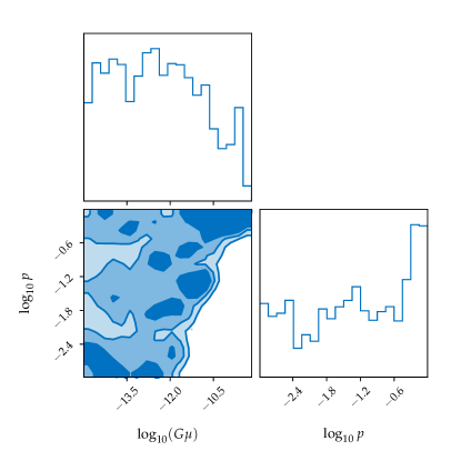
We first consider a model in which both the cosmic string tension and the reconnection probability are free parameters. Fig. 1 shows the posterior distributions of the and parameters obtained from the Bayesian search. The Bayes factor of the model including both the UCP and CS signal versus the model including only the UCP is , indicating no evidence for an SGWB signal produced by the cosmic string in the PPTA DR2.
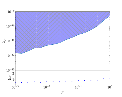
We also consider models in which the reconnection probability is fixed to a specific value while the cosmic string tension is allowed to vary. The lower panel of Fig. 2 shows the Bayes factor as a function of reconnection probability. For all the values of , we have , confirming that there is no evidence for an SGWB produced by cosmic strings in the PPTA DR2. We, therefore, place confidence level upper limit on cosmic string tension as a function of reconnection probability as shown in Fig. 2. The blue shaded region indicates parameter space that is excluded by the PPTA DR2. For , the upper bound on the cosmic string tension is , which is about five orders of magnitude tighter than the bound of Yonemaru et al. (2021) derived from the null search of individual gravitational wave burst from cosmic string cusps in the PPTA DR2. Note that is enhanced for , and therefore tighter constraints on are obtained for .
To sum up, we have searched for the SGWB produced by a cosmic string network in the PPTA DR2 in the work. We find no evidence for such SGWB signal, and therefore place upper limit on cosmic string tension as a function of reconnection probability.
Acknowledgements.
We thank Xing-Jiang Zhu, Zhi-Qiang You, Xiao-Jin Liu, Zhu Yi, and Shen-Shi Du for useful discussions. We acknowledge the use of HPC Cluster of ITP-CAS and HPC Cluster of Tianhe II in National Supercomputing Center in Guangzhou. This work is supported by the National Key Research and Development Program of China Grant No.2020YFC2201502, grants from NSFC (grant No. 11975019, 11991052, 12047503), Key Research Program of Frontier Sciences, CAS, Grant NO. ZDBS-LY-7009, CAS Project for Young Scientists in Basic Research YSBR-006, the Key Research Program of the Chinese Academy of Sciences (Grant NO. XDPB15).References
- Abbott et al. (2019) B. P. Abbott et al. (LIGO Scientific, Virgo), “GWTC-1: A Gravitational-Wave Transient Catalog of Compact Binary Mergers Observed by LIGO and Virgo during the First and Second Observing Runs,” Phys. Rev. X 9, 031040 (2019), arXiv:1811.12907 [astro-ph.HE] .
- Abbott et al. (2021a) R. Abbott et al. (LIGO Scientific, Virgo), “GWTC-2: Compact Binary Coalescences Observed by LIGO and Virgo During the First Half of the Third Observing Run,” Phys. Rev. X 11, 021053 (2021a), arXiv:2010.14527 [gr-qc] .
- Abbott et al. (2021b) R. Abbott et al. (LIGO Scientific, VIRGO), “GWTC-2.1: Deep Extended Catalog of Compact Binary Coalescences Observed by LIGO and Virgo During the First Half of the Third Observing Run,” (2021b), arXiv:2108.01045 [gr-qc] .
- Abbott et al. (2021c) R. Abbott et al. (LIGO Scientific, VIRGO, KAGRA), “GWTC-3: Compact Binary Coalescences Observed by LIGO and Virgo During the Second Part of the Third Observing Run,” (2021c), arXiv:2111.03606 [gr-qc] .
- Sazhin (1978) M. V. Sazhin, “Opportunities for detecting ultralong gravitational waves,” Soviet Astronomy 22, 36–38 (1978).
- Detweiler (1979) Steven L. Detweiler, “Pulsar timing measurements and the search for gravitational waves,” Astrophys. J. 234, 1100–1104 (1979).
- Foster and Backer (1990) R. S. Foster and D. C. Backer, “Constructing a Pulsar Timing Array,” Astrophys. J. 361, 300 (1990).
- Kramer and Champion (2013) Michael Kramer and David J. Champion, “The European Pulsar Timing Array and the Large European Array for Pulsars,” Class. Quant. Grav. 30, 224009 (2013).
- McLaughlin (2013) Maura A. McLaughlin, “The North American Nanohertz Observatory for Gravitational Waves,” Class. Quant. Grav. 30, 224008 (2013), arXiv:1310.0758 [astro-ph.IM] .
- Manchester et al. (2013) R. N. Manchester et al., “The Parkes Pulsar Timing Array Project,” Publ. Astron. Soc. Austral. 30, 17 (2013), arXiv:1210.6130 [astro-ph.IM] .
- Joshi et al. (2018) Bhal Chandra Joshi et al., “Precision pulsar timing with the ORT and the GMRT and its applications in pulsar astrophysics,” (2018), 10.1007/s12036-018-9549-y.
- Lee (2016) K. J. Lee, “Prospects of Gravitational Wave Detection Using Pulsar Timing Array for Chinese Future Telescopes,” in Frontiers in Radio Astronomy and FAST Early Sciences Symposium 2015, Astronomical Society of the Pacific Conference Series, Vol. 502, edited by L. Qain and D. Li (2016) p. 19.
- Bailes et al. (2020) M. Bailes et al., “The MeerKAT telescope as a pulsar facility: System verification and early science results from MeerTime,” Publ. Astron. Soc. Austral. 37, e028 (2020), arXiv:2005.14366 [astro-ph.IM] .
- Hobbs et al. (2010) G. Hobbs et al., “The international pulsar timing array project: using pulsars as a gravitational wave detector,” Gravitational waves. Proceedings, 8th Edoardo Amaldi Conference, Amaldi 8, New York, USA, June 22-26, 2009, Class. Quant. Grav. 27, 084013 (2010), arXiv:0911.5206 [astro-ph.SR] .
- Manchester (2013) R. N. Manchester, “The International Pulsar Timing Array,” Class. Quant. Grav. 30, 224010 (2013), arXiv:1309.7392 [astro-ph.IM] .
- Jaffe and Backer (2003) Andrew H. Jaffe and Donald C. Backer, “Gravitational waves probe the coalescence rate of massive black hole binaries,” Astrophys. J. 583, 616–631 (2003), arXiv:astro-ph/0210148 .
- Sesana et al. (2008) Alberto Sesana, Alberto Vecchio, and Carlo Nicola Colacino, “The stochastic gravitational-wave background from massive black hole binary systems: implications for observations with Pulsar Timing Arrays,” Mon. Not. Roy. Astron. Soc. 390, 192 (2008), arXiv:0804.4476 [astro-ph] .
- Sesana et al. (2009) A. Sesana, A. Vecchio, and M. Volonteri, “Gravitational waves from resolvable massive black hole binary systems and observations with Pulsar Timing Arrays,” Mon. Not. Roy. Astron. Soc. 394, 2255 (2009), arXiv:0809.3412 [astro-ph] .
- Saito and Yokoyama (2009) Ryo Saito and Jun’ichi Yokoyama, “Gravitational wave background as a probe of the primordial black hole abundance,” Phys. Rev. Lett. 102, 161101 (2009), [Erratum: Phys. Rev. Lett.107,069901(2011)], arXiv:0812.4339 [astro-ph] .
- Yuan et al. (2019a) Chen Yuan, Zu-Cheng Chen, and Qing-Guo Huang, “Probing Primordial-Black-Hole Dark Matter with Scalar Induced Gravitational Waves,” (2019a), arXiv:1906.11549 [astro-ph.CO] .
- Yuan et al. (2019b) Chen Yuan, Zu-Cheng Chen, and Qing-Guo Huang, “Log-dependent slope of scalar induced gravitational waves in the infrared regions,” (2019b), arXiv:1910.09099 [astro-ph.CO] .
- Chen et al. (2020) Zu-Cheng Chen, Chen Yuan, and Qing-Guo Huang, “Pulsar Timing Array Constraints on Primordial Black Holes with NANOGrav 11-Year Dataset,” Phys. Rev. Lett. 124, 251101 (2020), arXiv:1910.12239 [astro-ph.CO] .
- Yuan et al. (2019c) Chen Yuan, Zu-Cheng Chen, and Qing-Guo Huang, “Scalar Induced Gravitational Waves in Different Gauges,” (2019c), arXiv:1912.00885 [astro-ph.CO] .
- Chen et al. (2022) Zu-Cheng Chen, Chen Yuan, and Qing-Guo Huang, “Confronting the primordial black hole scenario with the gravitational-wave events detected by LIGO-Virgo,” Phys. Lett. B 829, 137040 (2022), arXiv:2108.11740 [astro-ph.CO] .
- Witten (1984) Edward Witten, “Cosmic Separation of Phases,” Phys. Rev. D 30, 272–285 (1984).
- Hogan (1986) C.J. Hogan, “Gravitational radiation from cosmological phase transitions,” Mon. Not. Roy. Astron. Soc. 218, 629–636 (1986).
- Lentati et al. (2015) L. Lentati et al., “European Pulsar Timing Array Limits On An Isotropic Stochastic Gravitational-Wave Background,” Mon. Not. Roy. Astron. Soc. 453, 2576–2598 (2015), arXiv:1504.03692 [astro-ph.CO] .
- Blanco-Pillado et al. (2018) Jose J. Blanco-Pillado, Ken D. Olum, and Xavier Siemens, “New limits on cosmic strings from gravitational wave observation,” Phys. Lett. B 778, 392–396 (2018), arXiv:1709.02434 [astro-ph.CO] .
- Arzoumanian et al. (2018a) Z. Arzoumanian et al. (NANOGRAV), “The NANOGrav 11-year Data Set: Pulsar-timing Constraints On The Stochastic Gravitational-wave Background,” Astrophys. J. 859, 47 (2018a), arXiv:1801.02617 [astro-ph.HE] .
- Yonemaru et al. (2021) N. Yonemaru et al., “Searching for gravitational wave bursts from cosmic string cusps with the Parkes Pulsar Timing Array,” Mon. Not. Roy. Astron. Soc. 501, 701–712 (2021), arXiv:2011.13490 [gr-qc] .
- Arzoumanian et al. (2020a) Zaven Arzoumanian et al. (NANOGrav), “The NANOGrav 12.5-year Data Set: Search For An Isotropic Stochastic Gravitational-Wave Background,” (2020a), arXiv:2009.04496 [astro-ph.HE] .
- Goncharov et al. (2021a) Boris Goncharov et al., “On the Evidence for a Common-spectrum Process in the Search for the Nanohertz Gravitational-wave Background with the Parkes Pulsar Timing Array,” Astrophys. J. Lett. 917, L19 (2021a), arXiv:2107.12112 [astro-ph.HE] .
- Chen et al. (2021a) S. Chen et al., “Common-red-signal analysis with 24-yr high-precision timing of the European Pulsar Timing Array: inferences in the stochastic gravitational-wave background search,” Mon. Not. Roy. Astron. Soc. 508, 4970–4993 (2021a), arXiv:2110.13184 [astro-ph.HE] .
- Antoniadis et al. (2022) J. Antoniadis et al., “The International Pulsar Timing Array second data release: Search for an isotropic gravitational wave background,” Mon. Not. Roy. Astron. Soc. 510, 4873–4887 (2022), arXiv:2201.03980 [astro-ph.HE] .
- Addazi et al. (2021) Andrea Addazi, Yi-Fu Cai, Qingyu Gan, Antonino Marciano, and Kaiqiang Zeng, “NANOGrav results and dark first order phase transitions,” Sci. China Phys. Mech. Astron. 64, 290411 (2021), arXiv:2009.10327 [hep-ph] .
- Ratzinger and Schwaller (2021) Wolfram Ratzinger and Pedro Schwaller, “Whispers from the dark side: Confronting light new physics with NANOGrav data,” SciPost Phys. 10, 047 (2021), arXiv:2009.11875 [astro-ph.CO] .
- Bian et al. (2021) Ligong Bian, Rong-Gen Cai, Jing Liu, Xing-Yu Yang, and Ruiyu Zhou, “Evidence for different gravitational-wave sources in the NANOGrav dataset,” Phys. Rev. D 103, L081301 (2021), arXiv:2009.13893 [astro-ph.CO] .
- Li et al. (2021) Shou-Long Li, Lijing Shao, Puxun Wu, and Hongwei Yu, “NANOGrav signal from first-order confinement-deconfinement phase transition in different QCD-matter scenarios,” Phys. Rev. D 104, 043510 (2021), arXiv:2101.08012 [astro-ph.CO] .
- Xue et al. (2021) Xiao Xue et al., “Constraining Cosmological Phase Transitions with the Parkes Pulsar Timing Array,” Phys. Rev. Lett. 127, 251303 (2021), arXiv:2110.03096 [astro-ph.CO] .
- Arzoumanian et al. (2021a) Zaven Arzoumanian et al. (NANOGrav), “Searching for Gravitational Waves from Cosmological Phase Transitions with the NANOGrav 12.5-Year Dataset,” Phys. Rev. Lett. 127, 251302 (2021a), arXiv:2104.13930 [astro-ph.CO] .
- Wang (2022) Deng Wang, “Novel Physics with International Pulsar Timing Array: Axionlike Particles, Domain Walls and Cosmic Strings,” (2022), arXiv:2203.10959 [astro-ph.CO] .
- Ferreira et al. (2022) Ricardo Z. Ferreira, Alessio Notari, Oriol Pujolas, and Fabrizio Rompineve, “Gravitational Waves from Domain Walls in Pulsar Timing Array Datasets,” (2022), arXiv:2204.04228 [astro-ph.CO] .
- Blasi et al. (2021) Simone Blasi, Vedran Brdar, and Kai Schmitz, “Has NANOGrav found first evidence for cosmic strings?” Phys. Rev. Lett. 126, 041305 (2021), arXiv:2009.06607 [astro-ph.CO] .
- Ellis and Lewicki (2021) John Ellis and Marek Lewicki, “Cosmic String Interpretation of NANOGrav Pulsar Timing Data,” Phys. Rev. Lett. 126, 041304 (2021), arXiv:2009.06555 [astro-ph.CO] .
- Chen et al. (2021b) Zu-Cheng Chen, Chen Yuan, and Qing-Guo Huang, “Non-tensorial gravitational wave background in NANOGrav 12.5-year data set,” Sci. China Phys. Mech. Astron. 64, 120412 (2021b), arXiv:2101.06869 [astro-ph.CO] .
- Arzoumanian et al. (2021b) Zaven Arzoumanian et al. (NANOGrav), “The NANOGrav 12.5-year Data Set: Search for Non-Einsteinian Polarization Modes in the Gravitational-wave Background,” Astrophys. J. Lett. 923, L22 (2021b), arXiv:2109.14706 [gr-qc] .
- Wu et al. (2022) Yu-Mei Wu, Zu-Cheng Chen, and Qing-Guo Huang, “Constraining the Polarization of Gravitational Waves with the Parkes Pulsar Timing Array Second Data Release,” Astrophys. J. 925, 37 (2022), arXiv:2108.10518 [astro-ph.CO] .
- Chen et al. (2021c) Zu-Cheng Chen, Yu-Mei Wu, and Qing-Guo Huang, “Searching for Isotropic Stochastic Gravitational-Wave Background in the International Pulsar Timing Array Second Data Release,” (2021c), arXiv:2109.00296 [astro-ph.CO] .
- Kibble (1976) T. W. B. Kibble, “Topology of Cosmic Domains and Strings,” J. Phys. A 9, 1387–1398 (1976).
- Vilenkin (1981) A. Vilenkin, “Gravitational radiation from cosmic strings,” Phys. Lett. B 107, 47–50 (1981).
- Vilenkin (1985) Alexander Vilenkin, “Cosmic Strings and Domain Walls,” Phys. Rept. 121, 263–315 (1985).
- Dvali and Vilenkin (2004) Gia Dvali and Alexander Vilenkin, “Formation and evolution of cosmic D strings,” JCAP 03, 010 (2004), arXiv:hep-th/0312007 .
- Copeland et al. (2004) Edmund J. Copeland, Robert C. Myers, and Joseph Polchinski, “Cosmic F and D strings,” JHEP 06, 013 (2004), arXiv:hep-th/0312067 .
- Blanco-Pillado and Olum (2017) Jose J. Blanco-Pillado and Ken D. Olum, “Stochastic gravitational wave background from smoothed cosmic string loops,” Phys. Rev. D 96, 104046 (2017), arXiv:1709.02693 [astro-ph.CO] .
- Kerr et al. (2020) Matthew Kerr et al., “The Parkes Pulsar Timing Array project: second data release,” Publ. Astron. Soc. Austral. 37, e020 (2020), arXiv:2003.09780 [astro-ph.IM] .
- Goncharov et al. (2021b) Boris Goncharov et al., “Identifying and mitigating noise sources in precision pulsar timing data sets,” Mon. Not. Roy. Astron. Soc. 502, 478–493 (2021b), arXiv:2010.06109 [astro-ph.HE] .
- Lentati et al. (2016) L. Lentati et al., “From Spin Noise to Systematics: Stochastic Processes in the First International Pulsar Timing Array Data Release,” Mon. Not. Roy. Astron. Soc. 458, 2161–2187 (2016), arXiv:1602.05570 [astro-ph.IM] .
- Chamberlin et al. (2015) Sydney J. Chamberlin, Jolien D. E. Creighton, Xavier Siemens, Paul Demorest, Justin Ellis, Larry R. Price, and Joseph D. Romano, “Time-domain Implementation of the Optimal Cross-Correlation Statistic for Stochastic Gravitational-Wave Background Searches in Pulsar Timing Data,” Phys. Rev. D 91, 044048 (2015), arXiv:1410.8256 [astro-ph.IM] .
- Hobbs et al. (2006) George Hobbs, R. Edwards, and R. Manchester, “Tempo2, a new pulsar timing package. 1. overview,” Mon. Not. Roy. Astron. Soc. 369, 655–672 (2006), arXiv:astro-ph/0603381 .
- Edwards et al. (2006) Russell T. Edwards, G. B. Hobbs, and R. N. Manchester, “Tempo2, a new pulsar timing package. 2. The timing model and precision estimates,” Mon. Not. Roy. Astron. Soc. 372, 1549–1574 (2006), arXiv:astro-ph/0607664 .
- Shannon and Cordes (2010) Ryan M. Shannon and James M. Cordes, “Assessing the Role of Spin Noise in the Precision Timing of Millisecond Pulsars,” Astrophys. J. 725, 1607–1619 (2010), arXiv:1010.4794 [astro-ph.SR] .
- Keith et al. (2013) M. J. Keith et al., “Measurement and correction of variations in interstellar dispersion in high-precision pulsar timing,” Mon. Not. Roy. Astron. Soc. 429, 2161 (2013), arXiv:1211.5887 [astro-ph.GA] .
- Lyne and Graham-Smith (2012) Andrew G. Lyne and Francis Graham-Smith, Pulsar astronomy, 48 (Cambridge University Press, 2012).
- Coles et al. (2015) W. A. Coles et al., “Pulsar Observations of Extreme Scattering Events,” Astrophys. J. 808, 113 (2015), arXiv:1506.07948 [astro-ph.SR] .
- Arzoumanian et al. (2016) Z. Arzoumanian et al. (NANOGrav), “The NANOGrav Nine-year Data Set: Limits on the Isotropic Stochastic Gravitational Wave Background,” Astrophys. J. 821, 13 (2016), arXiv:1508.03024 [astro-ph.GA] .
- Thrane and Romano (2013) Eric Thrane and Joseph D. Romano, “Sensitivity curves for searches for gravitational-wave backgrounds,” Phys. Rev. D 88, 124032 (2013), arXiv:1310.5300 [astro-ph.IM] .
- Hellings and Downs (1983) R. w. Hellings and G. s. Downs, “UPPER LIMITS ON THE ISOTROPIC GRAVITATIONAL RADIATION BACKGROUND FROM PULSAR TIMING ANALYSIS,” Astrophys. J. 265, L39–L42 (1983).
- Arzoumanian et al. (2020b) Zaven Arzoumanian et al. (NANOGrav), “The NANOGrav 12.5 yr Data Set: Search for an Isotropic Stochastic Gravitational-wave Background,” Astrophys. J. Lett. 905, L34 (2020b), arXiv:2009.04496 [astro-ph.HE] .
- Arzoumanian et al. (2018b) Z. Arzoumanian et al. (NANOGRAV), “The NANOGrav 11-year Data Set: Pulsar-timing Constraints On The Stochastic Gravitational-wave Background,” Astrophys. J. 859, 47 (2018b), arXiv:1801.02617 [astro-ph.HE] .
- Kass and Raftery (1995) Robert E. Kass and Adrian E. Raftery, “Bayes factors,” Journal of the American Statistical Association 90, 773–795 (1995).
- Carlin and Chib (1995) Bradley P. Carlin and Siddhartha Chib, “Bayesian model choice via markov chain monte carlo methods,” Journal of the Royal Statistical Society. Series B (Methodological) 57, 473–484 (1995).
- Godsill (2001) Simon J. Godsill, “On the relationship between markov chain monte carlo methods for model uncertainty,” Journal of Computational and Graphical Statistics 10, 230–248 (2001).
- Hee et al. (2016) Sonke Hee, Will Handley, Mike P. Hobson, and Anthony N. Lasenby, “Bayesian model selection without evidences: application to the dark energy equation-of-state,” Mon. Not. Roy. Astron. Soc. 455, 2461–2473 (2016), arXiv:1506.09024 [astro-ph.CO] .
- Taylor et al. (2020) Stephen R. Taylor, Rutger van Haasteren, and Alberto Sesana, “From Bright Binaries To Bumpy Backgrounds: Mapping Realistic Gravitational Wave Skies With Pulsar-Timing Arrays,” Phys. Rev. D 102, 084039 (2020), arXiv:2006.04810 [astro-ph.IM] .
- Folkner and Park (2018) William M. Folkner and Ryan S. Park, “Planetary ephemeris DE438 for Juno,” Tech. Rep. IOM392R-18-004, Jet Propulsion Laboratory, Pasadena, CA (2018).
- Ellis et al. (2020) Justin A. Ellis, Michele Vallisneri, Stephen R. Taylor, and Paul T. Baker, “Enterprise: Enhanced numerical toolbox enabling a robust pulsar inference suite,” Zenodo (2020).
- Taylor et al. (2021) Stephen R. Taylor, Paul T. Baker, Jeffrey S. Hazboun, Joseph Simon, and Sarah J. Vigeland, “enterprise_extensions,” (2021), v2.2.0.
- Ellis and van Haasteren (2017) Justin Ellis and Rutger van Haasteren, “jellis18/ptmcmcsampler: Official release,” (2017).
- Aggarwal et al. (2019) K. Aggarwal et al., “The NANOGrav 11-Year Data Set: Limits on Gravitational Waves from Individual Supermassive Black Hole Binaries,” Astrophys. J. 880, 2 (2019), arXiv:1812.11585 [astro-ph.GA] .