Promoting Saliency From Depth:
Deep Unsupervised RGB-D Saliency Detection

Abstract

Growing interests in RGB-D salient object detection (RGB-D SOD) have been witnessed in recent years, owing partly to the popularity of depth sensors and the rapid progress of deep learning techniques. Unfortunately, existing RGB-D SOD methods typically demand large quantity of training images being thoroughly annotated at pixel-level. The laborious and time-consuming manual annotation has become a real bottleneck in various practical scenarios. On the other hand, current unsupervised RGB-D SOD methods still heavily rely on handcrafted feature representations. This inspires us to propose in this paper a deep unsupervised RGB-D saliency detection approach, which requires no manual pixel-level annotation during training. It is realized by two key ingredients in our training pipeline. First, a depth-disentangled saliency update (DSU) framework is designed to automatically produce pseudo-labels with iterative follow-up refinements, which provides more trustworthy supervision signals for training the saliency network. Second, an attentive training strategy is introduced to tackle the issue of noisy pseudo-labels, by properly re-weighting to highlight the more reliable pseudo-labels. Extensive experiments demonstrate the superior efficiency and effectiveness of our approach in tackling the challenging unsupervised RGB-D SOD scenarios. Moreover, our approach can also be adapted to work in fully-supervised situation. Empirical studies show the incorporation of our approach gives rise to notably performance improvement in existing supervised RGB-D SOD models.

1 Introduction

The recent development of RGB-D salient object detection, i.e., RGB-D SOD, is especially fueled by the increasingly accessible 3D imaging sensors (Giancola et al., 2018) and their diverse applications, including image caption generation (Xu et al., 2015), image retrieval (Ko et al., 2004; Shao & Brady, 2006) and video analysis (Liu et al., 2008; Wang et al., 2018), to name a few. Provided with multi-modality input of an RGB image and its depth map, the task of RGB-D SOD is to effectively identify and segment the most distinctive objects in a scene.

The state-of-the-art RGB-D SOD approaches (Li et al., 2021a; Ji et al., 2020b; 2022; Chen et al., 2020b; Li et al., 2020b; 2021b) typically entail an image-to-mask mapping pipeline that is based on the powerful deep learning paradigms of e.g., VGG16 (Simonyan & Zisserman, 2015) or ResNet50 (He et al., 2016). This strategy has led to excellent performance. On the other hand, these RGB-D SOD methods are fully supervised, thus demand a significant amount of pixel-level training annotations. This however becomes much less appealing in practical scenarios, owing to the laborious and time-consuming process in obtaining manual annotations. It is therefore natural and desirable to contemplating unsupervised alternatives. Unfortunately, existing unsupervised RGB-D SOD methods, such as global priors (Ren et al., 2015), center prior (Zhu et al., 2017b), and depth contrast prior (Ju et al., 2014), rely primarily on handcrafted feature representations. This is in stark contrast to the deep representations learned by their supervised SOD counterparts, which in effect imposes severe limitations on the feature representation power that may otherwise benefit greatly from the potentially abundant unlabeled RGB-D images.

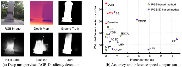
Figure 1: (a) An illustration of deep unsupervised RGB-D saliency detection. ‘Initial label’ is generated by a traditional method. ‘Baseline’ shows the saliency map generated by saliency network trained with initial pseudo-labels. ‘Ours’ shows our final results. (b) Efficiency and effectiveness comparison over a wide range of unsupervised SOD methods on the NLPR benchmark. Promoting Saliency From Depth: our approach achieves a large-margin improvement over the baseline, by engaging depth information to improve pseudo-labels in the training process, without introducing additional computational cost during inference, shown in red arrow.

These observations motivate us to explore a new problem of deep unsupervised RGB-D saliency detection: given an unlabeled set of RGB-D images, deep neural network is trained to predict saliency without any laborious human annotations in the training stage. A relatively straightforward idea is to exploit the outputs from traditional RGB-D method as pseudo-labels, which are internally employed to train the saliency prediction network (‘baseline’). Moreover, the input depth map may serve as a complementary source of information in refining the pseudo-labels, as it contains cues of spatial scene layout that may help in exposing the salient objects. Nevertheless, practical examination reveals two main issues: (1) Inconsistency and large variations in raw depth maps: as illustrated in Fig. 1 (a), similar depth values are often shared by a salient object and its surrounding, making it very difficult in extracting the salient regions from depth without explicit pixel-level supervision; (2) Noises from unreliable pseudo-labels: unreliable pseudo-labels may inevitably bring false positive into training, resulting in severe damage in its prediction performance.

To address the above challenges, the following two key components are considered in our approach. First, a depth-disentangled saliency update (DSU) framework is proposed to iteratively refine & update the pseudo-labels by engaging the depth knowledge. Here a depth-disentangled network is devised to explicitly learn the discriminative saliency cues and non-salient background from raw depth map, denoted as saliency-guided depth $D_{Sal}$ and non-saliency-guided depth $D_{NonSal}$, respectively. This is followed by a depth-disentangled label update (DLU) module that takes advantage of $D_{Sal}$ to emphasize saliency response from pseudo-label; it also utilizes $D_{NonSal}$ to eliminate the background influence, thus facilitating more trustworthy supervision signals in training the saliency network. Note the DSU module is not engaged at test time. Therefore, at test time, our trained model takes as input only an RGB image, instead of involving both RGB and depth as input and in the follow-up computation. Second, an attentive training strategy is introduced to alleviate the issue of noisy pseudo-labels; it is achieved by re-weighting the training samples in each training batch to focus on those more reliable pseudo-labels. As demonstrated in Fig. 1 (b), our approach works effectively and efficiently in practice. It significantly outperforms existing unsupervised SOD methods on the widely-used NLPR benchmark. Specifically, it improves over the baseline by 37%, a significant amount without incurring extra computation cost. Besides, the test time execution of our approach is at 35 frame-per-second (FPS), the fastest among all RGB-D unsupervised methods, and on par with the most efficient RGB-based methods. In summary, our main contributions are as follows:

• To our knowledge, our work is the first in exploring deep representation to tackle the problem of unsupervised RGB-D saliency detection. This is enabled by two key components in the training process, namely the DSU strategy to produce & refine pseudo-labels, and the attentive training strategy to alleviate the influence of noisy pseudo-labels. It results in a light-weight architecture that engages only RGB data at test time (i.e., w/o depth map), achieving a significant improvement without extra computation cost.

• Empirically, our approach outperforms state-of-the-art unsupervised methods on four public benchmarks. Moreover, it runs in real time at 35 FPS, much faster than existing unsupervised RGB-D SOD methods, and at least on par with the fastest RGB counterparts.

• Our approach could be adapted to work with fully-supervised scenario. As demonstrated in Sec. 4.4, augmented with our proposed DSU module, the empirical results of existing RGB-D SOD models have been notably improved.

2 Related Work

Remarkable progresses have been made recently in salient object detection (Ma et al., 2021; Xu et al., 2021; Pang et al., 2020b; Zhao et al., 2020b; Tsai et al., 2018; Liu et al., 2018), where the performance tends to deteriorate in the presence of cluttered or low-contrast backgrounds. Moreover, promising results are shown by a variety of recent efforts (Chen et al., 2021a; Luo et al., 2020; Chen et al., 2020a; Zhao et al., 2022; Desingh et al., 2013; Li et al., 2020a; Liao et al., 2020; Shigematsu et al., 2017) that integrate effective depth cues to tackle these issues. Those methods, however, typically demand extensive annotations, which are labor-intensive and time-consuming. This naturally leads to the consideration of unsupervised SODs that do not rely on such annotations.

Prior to the deep learning era (Wang et al., 2021; Zhao et al., 2020a), traditional RGB-D saliency methods are mainly based on the manually-crafted RGB features and depth cues to infer a saliency map. Due to their lack of reliance on manual human annotation, these traditional methods can be regarded as early manifestations of unsupervised SOD. Ju et al. (Ju et al., 2014) consider the incorporation of a prior induced from anisotropic center-surround operator, and an additional depth prior. Ren et al. (Ren et al., 2015) also introduce two priors: normalized depth prior and the global-context surface orientation prior. In contrary to direct utilization of the depth contrast priors, local background enclosure prior is explicitly developed by (Feng et al., 2016). Interested readers may refer to (Fan et al., 2020a; Peng et al., 2014; Zhou et al., 2021) for more in-depth surveys and analyses. However, by relying on manually-crafted priors, these methods tend to have inferior performance.

Meanwhile, considerable performance gain has been achieved by recent efforts in RGB-based unsupervised SOD (Zhang et al., 2017; 2018; Nguyen et al., 2019; Hsu et al., 2018a), which instead construct automated feature representations using deep learning. A typical strategy is to leverage the noisy output produced by traditional methods as pseudo-label (i.e., supervisory signal) for training saliency prediction net. The pioneering work of Zhang et al. (Zhang et al., 2017) fuses the outputs of multiple unsupervised saliency models as guiding signals in CNN training. In (Zhang et al., 2018), competitive performance is achieved by fitting a noise modeling module to the noise distribution of pseudo-label. Instead of directly using pseudo-labels from handcrafted methods, Nguyen et al. (Nguyen et al., 2019) further refine pseudo-labels via a self-supervision iterative process. Besides, deep unsupervised learning has been considered by (Hsu et al., 2018b; Tsai et al., 2019) for the co-saliency task, where superior performance has been obtained by engaging a fusion-learning scheme (Hsu et al., 2018b), or utilizing dedicated loss terms (Tsai et al., 2019). These methods demonstrate that the incorporation of powerful deep neural network brings better feature representation than those unsupervised SOD counterparts based on handcrafted features.

In this work, a principled research investigation on deep unsupervised RGB-D saliency detection. is presented for the first time. Different from existing deep RGB-based unsupervised SOD  (Zhang et al., 2017; 2018) that use pseudo-labels from the handcrafted methods directly, our work aims to refine and update pseudo-labels to remove the undesired noise. And compared to the refinement method (Nguyen et al., 2019) using self-supervision technique, our approach instead adopts disentangled depth information to promote pseudo-labels.

3 Methodology

3.1 Overview

Fig. 2 presents an overview of our Depth-disentangled Saliency Update (DSU) framework. Overall our DSU strives to significantly improve the quality of pseudo-labels, that leads to more trustworthy supervision signals for training the saliency network. It consists of three key components. First is a saliency network responsible for saliency prediction, whose initial supervision signal is provided by traditional handcrafted method without using human annotations. Second, a depth network and a depth-disentangled network are designed to decompose depth cues into saliency-guided depth $D_{Sal}$ and non-saliency-guided depth $D_{NonSal}$, to explicitly depict saliency cues in the spatial layout. Third, a depth-disentangled label update (DLU) module is devised to refine and update the pseudo-labels, by engaging the learned $D_{Sal}$ and $D_{NonSal}$. The updated pseudo-labels could in turn provide more trustworthy supervisions for the saliency network. Moreover, an attentive training strategy (ATS) is incorporated when training the saliency network, tailored for noisy unsupervised learning by mitigating the ambiguities caused by noisy pseudo-labels. We note that the DSU and ATS are not performed at test time, so does not affect the inference speed. In other words, the inference stage involves only the black dashed portion of the proposed network architecture in Fig. 2, i.e., only RGB images are used for predicting saliency, which enables very efficient detection.

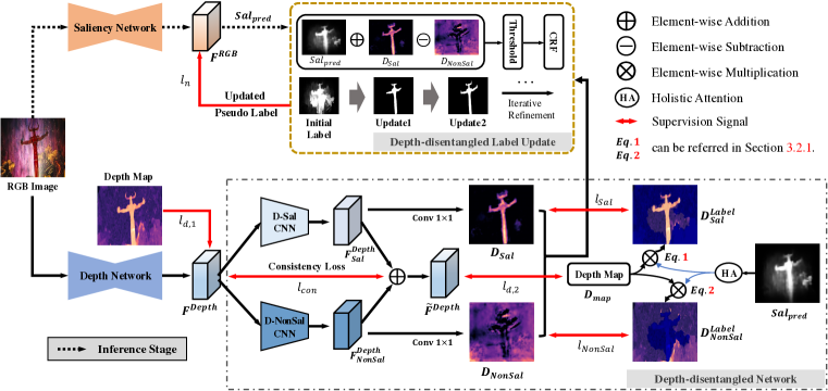
Figure 2: Overview of the proposed method. The saliency network is trained with the iteratively updated pseudo-labels. The depth network and depth-disentangled network are designed to decompose raw depth into saliency-guided depth $D_{Sal}$ and non-saliency-guided depth $D_{NonSal}$, which are subsequently fed into the depth-disentangled label update (DLU) module to refine and update pseudo-labels. The inference stage involves only the black dashed portion.

3.2 Depth-disentangled Saliency Update

The scene geometry embedded in the depth map can serve as a complementary information source to refine the pseudo-labels. Nevertheless, as discussed in the introduction section, a direct adoption of the raw depth may not necessarily lead to good performance due to the large value variations and inherit noises in raw depth map. Without explicit pixel-wise supervision, the saliency model may unfortunately be confused by nearby background regions having the same depth but with different contexts; meanwhile, depth variations in salient or background regions may also result in false responses. These observations motivate us to design a depth-disentangled network to effectively capture discriminative saliency cues from depth, and a depth-disentangled label update (DLU) strategy to improve and refine pseudo-labels by engaging the disentangled depth knowledges.

3.2.1 Depth-disentangled Network

The depth-disentangled network aims at capturing valuable saliency as well as redundant non-salient cues from raw depth map. As presented in the bottom of Fig. 2, informative depth feature $F^{Depth}$ is first extracted from the depth network under the supervision of raw depth map, using the mean square error (MSE) loss function, i.e., $l_{d,1}$. The $F^{Depth}$ is then decomposed into saliency-guided depth $D_{Sal}$ and non-saliency-guided depth $D_{NonSal}$ following two principles: 1) explicitly guiding the model to learn saliency-specific cues from depth; 2) ensuring the coherence between the disentangled and original depth features.

Specifically, in the bottom right of Fig. 2, we first construct the spatial supervision signals for the depth-disentangled network. Given the rough saliency prediction $Sal_{pred}$ from the saliency network and the raw depth map $D_{map}$, the (non-)saliency-guided depth masks, i.e., $D_{Sal}^{Label}$ and $D_{NonSal}^{Label}$, can be obtained by multiplying $Sal_{pred}$ (or $1-Sal_{pred}$) and depth map $D_{map}$ in a spatial attention manner. Since the predicted saliency may contain errors introduced from the inaccurate pseudo-labels, we employ a holistic attention (HA) operation (Wu et al., 2019) to smooth the coverage area of the predicted saliency, so as to effectively perceive more saliency area from depth. Formally, the (non-)saliency-guided depth masks are generated by:

$$D_{Sal}^{Label}=\Psi_{\max}(\mathcal{F}_{G}(Sal_{pred},k),Sal_{pred})\otimes D_{map},$$ (1)

$$D_{NonSal}^{Label}=\Psi_{\max}(\mathcal{F}_{G}(1-Sal_{pred},k),1-Sal_{pred})\otimes D_{map},$$ (2)

where $\mathcal{F}_{G}(\cdot,k)$ represents the HA operation, which is implemented using the convolution operation with Gaussian kernel $k$ and zero bias; the size and standard deviation of the Gaussian kernel $k$ are initialized with 32 and 4, respectively, which are then finetuned through the training procedure; $\Psi_{\max}(\cdot,\cdot)$ is a maximum function to preserve the higher values from the Gaussian filtered map and the original map; $\otimes$ denotes pixel-wise multiplication.

Building upon the guidance of $D_{Sal}^{Label}$ and $D_{NonSal}^{Label}$, $F^{Depth}$ is fed into D-Sal CNN and D-NonSal CNN to explicitly learn valuable saliency and redundant non-salient cues from depth map, generating $D_{Sal}$ and $D_{NonSal}$, respectively. The loss functions here (i.e., $l_{Sal}$ and $l_{NonSal}$) are MSE loss. Detailed structures of D-Sal and D-NonSal CNNs are in the appendix. To further ensure the coherence between the disentangled and original depth features, a consistency loss, ${l}_{con}$, is employed as:

$${{l}}_{con}={\frac{1}{{H}{\times}{W}{\times}{C}}}{\sum_{i=1}^{H}\sum_{j=1}^{W}\sum_{k=1}^{C}{\parallel}{F}_{i,j,k}^{Depth},\tilde{F}_{i,j,k}^{Depth}{\parallel}_{2}},$$ (3)

where $\tilde{F}^{Depth}$ is the sum of the disentangled ${F}^{Depth}_{Sal}$ and ${F}^{Depth}_{NonSal}$, which denotes the regenerated depth feature; $H$, $W$ and $C$ are the height, width and channel of ${F}^{Depth}$ and $\tilde{F}^{Depth}$; ${\parallel}{\cdot}{\parallel}_{2}$ represents Euclidean norm. Here, $\tilde{F}^{Depth}$ is also under the supervision of depth map, using MSE loss, i.e., $l_{d,2}$.

Then, the overall training objective for the depth network and the depth-disentangled network is as:

$$\mathcal{L}_{depth}=\frac{1}{5N}\sum_{n=1}^{N}(l_{d,1}^{n}+l_{d,2}^{n}+l_{Sal}^{n}+l_{NonSal}^{n}+{\lambda}l_{con}^{n}),$$ (4)

where $n$ denotes the $n_{th}$ sample in a mini-batch with $N$ training samples; $\lambda$ is set to 0.02 in the experiments to balance the consistency loss $l_{con}$ and other loss terms. As empirical evidences in Fig. 3 suggested, comparing to the raw depth map, $D_{Sal}$ is better at capturing discriminative cues of the salient objects, while $D_{NonSal}$ better depicts the complementary background context.

In the next step, the learned $D_{Sal}$ and $D_{NonSal}$ are fed into our Depth-disentangled Label Update, to obtain the improved pseudo-labels.

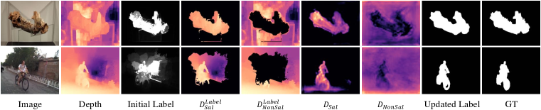
Figure 3: The internal inspections of the proposed DSU. It is observed that the updated label exhibits more reliable saliency signals than initial pseudo-label.

3.2.2 Depth-disentangled Label Update

To maintain more reliable supervision signals in training, a depth-disentangled label update (DLU) strategy is devised to iteratively refine & update pseudo-labels. Specifically, as shown in the upper stream of Fig. 2, using the obtained $Sal_{pred}$, $D_{Sal}$ and $D_{NonSal}$, the DLU simultaneously highlights the salient regions in the coarse saliency prediction by the sum of $Sal_{pred}$ and $D_{Sal}$, and suppresses the non-saliency negative responses by subtracting $D_{NonSal}$ in a pixel-wise manner. This process can be formulated as:

$$\mathcal{S}_{temp}=Sal_{pred}^{i,j}+D_{Sal}^{i,j}-D_{NonSal}^{i,j}\bigg{|}_{i\in[1,H];j\in[1,W]}.$$ (5)

To avoid the value overflow of the obtained $\mathcal{S}_{temp}$ (i.e., removing negative numbers and normalizing the results to the range of [0, 1]), a thresholding operation and a normalization process are performed as:

$$\mathcal{S}_{\mathcal{N}}=\frac{\mathcal{S}_{n}^{i,j}-min(\mathcal{S}_{n})}{max(\mathcal{S}_{n})-min(\mathcal{S}_{n})},{\rm where}\ \mathcal{S}_{n}=\begin{cases}0,&\mbox{if }\mathcal{S}_{temp}^{i,j}<0\\ \mathcal{S}_{temp}^{i,j},&\mbox{others}\end{cases},i\in[1,H];j\in[1,W],$$ (6)

where $min(\cdot)$ and $max(\cdot)$ denote the minimum and maximum functions. Finally, a fully-connected conditional random field (CRF (Hou et al., 2017)) is applied to $\mathcal{S}_{\mathcal{N}}$, to generate the enhanced saliency map $\mathcal{S}_{map}$ as the updated pseudo-labels. The empirical result of the proposed DSU step is showcased in Fig. 3, with quantitative results presented in Table 6. These internal evidences suggest that the DSU leads to noticeable improvement after merely several iterations.

3.3 Attentive Training Strategy

When training the saliency network using pseudo-labels, an attentive training strategy (ATS) is proposed to tailor for the deep unsupervised learning context, to reduce the influence of ambiguous pseudo-labels, and concentrate on the more reliable training examples. This strategy is inspired by the human learning process of understanding new knowledge, that is, from general to specific understanding cycle (Dixon, 1999; Peltier et al., 2005). The ATS alternates between two steps to re-weigh the training instances in a mini-batch.

To be specific, we first start by settling the related loss functions. For the $n_{th}$ sample in a mini-batch with $N$ training samples, we define the binary cross-entropy loss between the predicted saliency $Sal_{pred}^{n}$ and the pseudo-label $\mathcal{S}_{map}^{n}$ as:

$$l_{n}=-(\mathcal{S}_{map}^{n}\cdot\log{Sal_{pred}^{n}}+(1-\mathcal{S}_{map}^{n})\cdot\log(1-Sal_{pred}^{n})).$$ (7)

Then, the training objective for the saliency network in current mini-batch is defined as an attentive binary cross-entropy loss $\mathcal{L}_{sal}$, which can be represented as follows:

$$\mathcal{L}_{sal}=\frac{1}{\sum_{n=1}^{N}\alpha_{n}}\sum_{n=1}^{N}(\alpha_{n}\cdot l_{n}),\mathcal{\alpha}_{n}=\begin{cases}1,&\mbox{step one,}\\ \frac{\sum_{i\in N}^{i\neq n}e^{l_{i}}}{\sum_{i\in N}e^{l_{i}}},&\mbox{step two,}\end{cases}$$ (8)

where $\alpha_{n}$ represents the weight of the $n_{th}$ training sample at current training mini-batch.

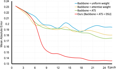
Figure 4: Analysis of the proposed attentive training strategy, when evaluated on NJUD testset. The ‘backbone’ refers to the saliency network trained with initial pseudo-labels.

The ATS starts from a uniform weight for each training sample in step one to learn general representations across a lot of training data. Step two decreases the importance of ambiguous training instances through the imposed attentive loss; the higher the loss value, the less weight an instance is to get.

In this paper, we define step one and two as a training round ($2\tau$ epochs). During each training round, the saliency loss $\mathcal{L}_{sal}$ and depth loss $\mathcal{L}_{depth}$ are optimized simultaneously to train their network parameters. The proposed DLU is taken at the end of each training round to update the pseudo-labels for the saliency network; meanwhile, $D_{Sal}^{Label}$ and $D_{NonSal}^{Label}$ in Eqs.1 and 2 are also updated using the improved $Sal_{pred}$. This allows the network to make efficient use of the updated pseudo labels. As suggested by Fig. 4 and Table 3, the use of our attentive training strategy leads to more significant error reduction compared with the backbone solely using uniform weight or attentive weight for each instance. Besides, when our DSU and the attentive training strategy are both incorporated to the backbone, better results are achieved.

4 Experiments and Analyses

4.1 Datasets and Evaluation Metrics

Extensive experiments are conducted over four large-scale RGB-D SOD benchmarks. NJUD (Ju et al., 2014) in its latest version consists of 1,985 samples, that are collected from the Internet and 3D movies; NLPR (Peng et al., 2014) has 1,000 stereo images collected with Microsoft Kinect; STERE (Niu et al., 2012) contains 1,000 pairs of binocular images downloaded from the Internet; DUTLF-Depth (Piao et al., 2019) has 1,200 real scene images captured by a Lytro2 camera. We follow the setup of (Fan et al., 2020a) to construct the training set, which includes 1,485 samples from NJUD and 700 samples from NLPR, respectively. Data augmentation is also performed by randomly rotating, cropping and flipping the training images to avoid potential overfitting. The remaining images are reserved for testing.

Here, five widely-used evaluation metrics are adopted: E-measure ($E_{\xi}$) (Fan et al., 2018), weighed F-measure ($F_{\beta}^{w}$) (Margolin et al., 2014), F-measure ($F_{\beta}$) (Achanta et al., 2009), Mean Absolute Error (MAE or $\mathcal{M}$) (Borji et al., 2015), and inference time(s) or FPS (Frames Per Second).

Implementation details are presented in the Appx A.3. Source code is publicly available.

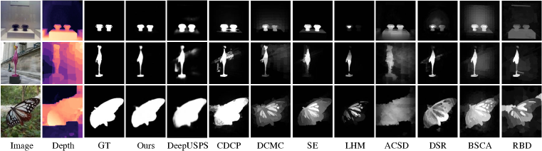
Figure 5: Qualitative comparison with unsupervised saliency detection methods. GT denotes ground-truth.

Table 1: Quantitative comparison with unsupervised SOD methods. ‘Backbone’ refers to the saliency feature extraction network  (Wu et al., 2019) adopted in our pipeline, i.e. the one without the two proposed key components. The RGB-based methods are specifically marked by ^†. UnSOD is shorthand for unsupervised SOD. We also provide the results of existing fully supervised methods that can be referenced in Table 8.

*		Inference	NJUD				NLPR				STERE				DUTLF-Depth
		Time(s)$\downarrow$	$E_{\xi}\uparrow$	$F_{\beta}^{w}\uparrow$	$F_{\beta}\uparrow$	$\mathcal{M}\downarrow$	$E_{\xi}\uparrow$	$F_{\beta}^{w}\uparrow$	$F_{\beta}\uparrow$	$\mathcal{M}\downarrow$	$E_{\xi}\uparrow$	$F_{\beta}^{w}\uparrow$	$F_{\beta}\uparrow$	$\mathcal{M}\downarrow$	$E_{\xi}\uparrow$	$F_{\beta}^{w}\uparrow$	$F_{\beta}\uparrow$	$\mathcal{M}\downarrow$
Handcrafted UnSOD	RBD† (Zhu et al., 2014)	0.189	.684	.387	.556	.256	.765	.388	.590	.211	.730	.443	.610	.223	.733	.447	.619	.222
	MST† (Tu et al., 2016)	0.030	.670	.291	.436	.281	.762	.257	.491	.199	.681	.312	.447	.269	.678	.254	.401	.279
	BSCA† (Qin et al., 2015)	2.665	.756	.446	.623	.216	.745	.376	.554	.178	.803	.497	.676	.179	.808	.479	.682	.181
	DSR† (Li et al., 2013)	0.376	.739	.436	.594	.196	.757	.451	.545	.120	.785	.486	.645	.165	.797	.478	.640	.164
	ACSD (Ju et al., 2014)	0.718	.790	.448	.696	.198	.751	.327	.547	.171	.793	.425	.661	.200	.250	.210	.188	.668
	DES (Cheng et al., 2014)	7.790	.421	.241	.165	.448	.735	.259	.583	.301	.673	.383	.592	.297	.733	.386	.668	.280
	LHM (Peng et al., 2014)	2.130	.722	.311	.625	.201	.772	.320	.520	.119	.772	.360	.703	.171	.767	.350	.659	.174
	GP (Ren et al., 2015)	12.98	.730	.323	.666	.204	.813	.347	.670	.144	.785	.371	.710	.182	-	-	-	-
	CDB (Liang et al., 2018)	0.600	.752	.408	.650	.200	.810	.388	.618	.108	.808	.436	.713	.166	-	-	-	-
	SE (Guo et al., 2016)	1.570	.780	.518	.735	.164	.853	.578	.701	.085	.825	.546	.747	.143	.730	.339	.474	.196
	DCMC (Cong et al., 2016)	1.210	.796	.506	.715	.167	.684	.265	.328	.196	.832	.529	.743	.148	.712	.290	.406	.243
	MB (Zhu et al., 2017a)	-	.643	.369	.492	.202	.814	.574	.637	.089	.693	.455	.572	.178	.691	.464	.577	.156
	CDCP (Zhu et al., 2017b)	5.720	.751	.522	.618	.181	.785	.512	.591	.114	.797	.596	.666	.149	.794	.530	.633	.159
Deep UnSOD	USD† (Zhang et al., 2018)	0.0180	.768	.565	.630	.163	.786	.536	.580	.119	.796	.572	.670	.146	.795	.545	.650	.157
	DeepUSPS† (Nguyen et al., 2019)	0.0292	.771	.576	.647	.159	.809	.622	.639	.088	.806	.632	.682	.124	.798	.573	.654	.149
	Backbone	0.0286	.759	.510	.627	.186	.760	.479	.570	.126	.794	.555	.666	.158	.798	.512	.644	.167
	$\Delta$ gains	-	$\uparrow$5%	$\uparrow$17%	$\uparrow$15%	$\downarrow$27%	$\uparrow$16%	$\uparrow$37%	$\uparrow$31%	$\downarrow$48%	$\uparrow$8%	$\uparrow$22%	$\uparrow$16%	$\downarrow$37%	$\uparrow$7%	$\uparrow$27%	$\uparrow$18%	$\downarrow$36%
	Ours	0.0286	.797	.597	.719	.135	.879	.657	.745	.065	.857	.678	.774	.099	.854	.650	.763	.107

4.2 Comparison with the State-of-the-arts

Our approach is compared with 15 unsupervised SOD methods, i.e., without using any human annotations. Their results are either directly furnished by the authors of the respective papers, or generated by re-running their original implementations. In this paper, we make the first attempt to address deep-learning-based unsupervised RGB-D SOD. Since existing unsupervised RGB-D methods are all based on handcrafted feature representations, we additionally provide several RGB-based methods (e.g., USD and DeepUSPS) for reference purpose only. This gives more observational evidences for the related works. These RGB-based methods are specifically marked by ^† in Table 1.

Quantitative results are listed in Table 1, where our approach clearly outperforms the state-of-the-art unsupervised SOD methods in both RGB-D and RGB only scenarios. This is due to our DSU framework that leads to trustworthy supervision signals for saliency network. Furthermore, our network design leads to a light-weight architecture in the inference stage, shown as the black dashed portion in Fig. 2. This enables efficient & effective detection of salient objects and brings a large-margin improvement over the backbone network without introducing additional depth input and computational costs, as shown in Fig. 1 and Table 1. Qualitatively, saliency predictions of competing methods are exhibited in Fig. 5. These results consistently proves the superiority of our method.

4.3 Analysis of the Empirical Results

The focus here is on the evaluation of the contributions from each of the components, and the evaluation of the obtained pseudo-labels as intermediate results.

Effect of each component. In Table 2, we conduct ablation study to investigate the contribution of each component. To start with, we consider the backbone (a), where the saliency network is trained with initial pseudo-labels. As our proposed ATS and DSU are gradually incorporated, increased performance has been observed on both datasets. Here we first investigate the benefits of ATS by applying it to the backbone and obtaining (b). We observe increased F-measure scores of 3% and 5.8% on NJUD and NLPR benchmarks, respectively. This clearly shows that the proposed ATS can effectively improve the utilization of reliable pseudo-labels, by re-weighting ambiguous training data. We then investigate in detail all components in our DSU strategy. The addition of the entire DSU leads to (f), which significantly improves the F-measure metric by 11.3% and 23.5% on each of the benchmarks, while reducing the MAE by 22.4% and 41.9%, respectively. This verifies the effectiveness of the DSU strategy to refine and update pseudo-labels. Moreover, as we gradually exclude the consistency loss ${l}_{con}$ (row (e)) and HA operation (row (d)), degraded performances are observed on both datasets. For an extreme case where we remove the DLU and only maintain CRF to refine pseudo-labels, it is observed that much worse performance is achieved. These results consistently demonstrate that all components in the DSU strategy are beneficial for generating more accurate pseudo-labels.

Table 2: Ablation study of our deep unsupervised RGB-D SOD pipeline, using the F-measure and MAE metrics.

Index	Model Setups		NJUD		NLPR
			$F_{\beta}\uparrow$	$\mathcal{M}\downarrow$	$F_{\beta}\uparrow$	$\mathcal{M}\downarrow$
(a)	Backbone		0.627	0.186	0.570	0.126
(b)	(a) + attentive training strategy		0.646	0.174	0.603	0.112
(c)		(b) + CRF	0.674	0.160	0.663	0.093
(d)	DSU strategy	(b) + DSU (w/o ${l}_{con}\&HA$)	0.703	0.141	0.716	0.074
(e)		(b) + DSU (w/o ${l}_{con}$)	0.712	0.137	0.735	0.068
(f)		(b) + DSU (Ours)	0.719	0.135	0.745	0.065

We also display the visual evidence of the updated pseudo-labels obtained from the DSU strategy in Fig. 6. It is shown that the initial pseudo-labels unfortunately tend to miss important parts as well as fine-grained details. The application of CRF helps to filter away background noises, while salient parts could still be missing out. By adopting our DSU and attentive training strategy, the missing parts could be retrieved in the updated pseudo-labels, with the object silhouette also being refined. These numerical and visual results consistently verify the effectiveness of our pipeline in deep unsupervised RGB-D saliency detection.

Table 3: Analyzing attentive training strategy (ATS) with different settings. ‘Setting 1’ is backbone + uniform weight + DSU, and ‘Setting 2’ is backbone + attentive weight + DSU. The last four columns show backbone + ATS + DSU with different alternation interval $\tau$.

*		Analysis of the ATS		Ours	Analysis of the interval $\tau$
		Setting 1	Setting 2	$\tau=3$	$\tau=1$	$\tau=5$	$\tau=10$
NJUD	$F_{\beta}\uparrow$	0.695	0.707	0.719	0.711	0.712	0.687
	$\mathcal{M}\downarrow$	0.148	0.142	0.135	0.143	0.138	0.147
NLPR	$F_{\beta}\uparrow$	0.706	0.737	0.745	0.742	0.739	0.698
	$\mathcal{M}\downarrow$	0.071	0.067	0.065	0.069	0.066	0.073

Detailed analysis of the ATS. The influence of the attentive training strategy (ATS) is studied in detail here. The error reduction curves in Fig. 4 have shown that the use of ATS could lead to greater test error reduction compared with the backbone that uses uniform weight or attentive weight for each instance. When combining the ATS with the DSU strategy as shown in Table 3, the ATS also enables the network to learn more efficiently than using uniform weight or attentive weight alone, by comparing ‘Ours’ with ‘Setting 1’ and ‘Setting 2’. In addition, we discuss the effect of different alternation intervals $\tau$ in ATS. As listed in Table 3, the larger or smaller interval leads to inferior performance due to the insufficient or excessive learning of saliency models.

Table 4: Internal mean absolute errors, each is evaluated between current pseudo-labels and the corresponding true labels (only used for evaluation purpose) during the training process.

Pseudo-label Update	Initial	Update 1	Update 2	Update 3	Update 4
Mean absolute error	0.162	0.124	0.117	0.116	0.116

Table 5: Comparison of different pseudo-label generation variants. ‘CRF’ refers to fully-connected CRF. ‘OTSU’ represents the standard Otsu image thresholding method.

Label Accuray	$E_{\xi}\uparrow$	$F_{\beta}^{w}\uparrow$	$F_{\beta}\uparrow$	$\mathcal{M}\downarrow$
Initial pseudo-label	0.760	0.526	0.614	0.162
Initial pseudo-label + CRF	0.763	0.578	0.634	0.144
Our DSU	0.792	0.635	0.708	0.116
Depth map	0.419	0.284	0.164	0.414
Depth map + OTSU	0.465	0.398	0.429	0.332

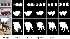
Figure 6: Visual examples of the intermediate pseudo-labels used in our approach. ‘Initial’ shows the initial pseudo-labels generated by traditional handcrafted method. ‘+CRF’ refers to the pseudo-labels after applying fully-connected CRF. Update 1&2 represent the updated pseudo-labels produced in our pipeline over two training rounds. ‘GT’ means the ground truth, used for reference purpose only.

Analysis of pseudo-labels. We analyze the quality of pseudo-labels over the training process in Table 6, where the mean absolute error scores between the pseudo-labels at different update rounds and the ground-truth labels are reported. It is observed that the quality of pseudo-labels is significantly improved during the first two rounds, which then remains stable in the consecutive rounds. Fig. 6 also shows that the initial pseudo-label is effectively refined, where the updated pseudo-label is close to the true label. This provides more reliable guiding signals for training the saliency network.

Comparison of different pseudo-label variants. In Table 6, we investigate other possible pseudo-label generation variants, including, initial pseudo-label with CRF refinement, raw depth map, and raw depth map together with OTSU thresholding (Otsu, 1979). It is shown that, compared with the direct use of CRF, our proposed DSU is able to provide more reliable pseudo-labels, by disentangling depth to promote saliency. It is worth noting that a direct application of the raw depth map or together with an OTSU adaptive thresholding of the depth map, may nevertheless lead to awful results. We conjecture this is because of the large variations embedded in raw depth, and the fact that foreground objects may be affected by nearby background stuffs that are close in depth.

Table 6: Discussion on different pseudo-label updating settings.

Different Pseudo-label Updating Setups		NJUD		NLPR
		$F_{\beta}\uparrow$	$\mathcal{M}\downarrow$	$F_{\beta}\uparrow$	$\mathcal{M}\downarrow$
(a) DSU w/o $D_{NonSal}$		0.698	0.143	0.715	0.072
(b) DSU using $D^{Label}_{Sal}$, $D^{Label}_{NonSal}$		0.691	0.154	0.707	0.079
(c) DSU using $D_{Sal}$, $D_{NonSal}$ (Ours)		0.719	0.135	0.745	0.065

Is depth-disentanglement necessary? In our DSU, we disentangle the raw depth map into valuable salient parts as well as redundant non-salient areas to simultaneously highlight the salient regions and suppress the non-salient negative responses. To verify the necessity of depth disentanglement, we remove the $D_{NonSal}$ branch in the depth-disentangled network and only use the $D_{Sal}$ to update pseudo-labels in DLU. Empirical results in Table 6 reveal that removing $D_{NonSal}$ (row (a)) leads to significant inferior performance when comparing with the original DSU (row (c)), which proves the superiority of our DSU design.

How about using raw depth labels in DSU? We also consider to directly utilize the raw disentangled depth labels, i.e., $D^{Label}_{Sal}$ and $D^{Label}_{NonSal}$, to update pseudo-labels in DSU. However, a direct adoption of the raw depth labels does not lead to good performance, as empirically exhibited in Table 6 (b). The DSU using raw labels performs worse compared to our original DSU design in row (c). This is partly due to the large value variations and intrinsic label noises in raw depth map as discussed before. On the other hand, benefiting from the capability of deep-learning-based networks to learn general representations from large-scale data collections, using $D_{Sal}$ and $D_{NonSal}$ in our DSU strategy is able to eliminate the potential biases in a single raw depth label. Visual evidences as exhibited in the 4^th-7^th columns of Fig. 3 also support our claim.

4.4 Application to Fully-supervised Setting

Table 7: Applying our DSU to existing fully-supervised RGB-D SOD methods.

*	NJUD		NLPR
	$F_{\beta}\uparrow$	$\mathcal{M}\downarrow$	$F_{\beta}\uparrow$	$\mathcal{M}\downarrow$
DMRA (Piao et al., 2019)	0.872	0.051	0.855	0.031
+ Our DSU	0.893	0.044	0.879	0.026
CMWN (Li et al., 2020c)	0.878	0.047	0.859	0.029
+ Our DSU	0.901	0.041	0.882	0.025
FRDT (Zhang et al., 2020f)	0.879	0.048	0.868	0.029
+ Our DSU	0.903	0.038	0.901	0.023
CPD (Wu et al., 2019)	0.873	0.045	0.866	0.028
+ Our DSU	0.909	0.036	0.907	0.022

To show the generic applicability of our approach, a variant of our DSU is applied to several cutting-edge fully-supervised SOD models to improve their performance. This is made possible by redefining the quantities $D^{Label}_{Sal}=\mathcal{S}_{GT}\otimes D_{map}$ and $D^{Label}_{NonSal}=(1-\mathcal{S}_{GT})\otimes D_{map}$, with $\mathcal{S}_{GT}$ being the ground-truth saliency. Then the saliency network (i.e., existing SOD models) and the depth-disentangled network are retrained by $\mathcal{S}_{GT}$ and the new $D^{Label}_{Sal}$ and $D^{Label}_{NonSal}$, respectively. After training, the proposed DLU is engaged to obtain the final improved saliency. In Table 7, we report the original results of four SOD methods and the new results of incorporating our DSU strategy on two popular benchmarks. It is observed that our supervised variants have consistent performance improvement comparing to each of existing models. For example, the average MAE score of four SOD methods on NJUD benchmark is reduced by 18.0%. We attribute the performance improvement to our DSU strategy that can exploit the learned $D_{Sal}$ to facilitate the localization of salient object regions in a scene, as well as suppress the redundant background noises by subtracting $D_{NonSal}$. More experiments are presented in the Appx A.2.

5 Conclusion and Outlook

This paper tackles the new task of deep unsupervised RGB-D saliency detection. Our key insight is to internally engage and refine the pseudo-labels. This is realized by two key modules, the depth-disentangled saliency update in iteratively fine-tuning the pseudo-labels, and the attentive training strategy in addressing the issue of noisy pseudo-labels. Extensive empirical experiments demonstrate the superior performance and realtime efficiency of our approach. For future work, we plan to extend our approach to scenarios involving partial labels.
Acknowledgement. This research was partly supported by the University of Alberta Start-up Grant, UAHJIC Grants, and NSERC Discovery Grants (No. RGPIN-2019-04575).

Appendix A Appendix

In this appendix, we first elaborate on the evaluation metrics used in this paper, in Appx A.1. Then, more details and experiments of our DSU are presented in Appx A.2, including the detailed structures of D-Sal and D-NonSal CNNs, more experiments on unsupervised and fully-supervised scenarios, and other pseudo-label initialization. These empirical results consistently demonstrate the effectiveness and scalability of our approach. In Appx A.3, we illustrate on the implementation details of our unsupervised pipeline. In Appx A.4, we discuss the potential limitations which can be addressed in the near future. In Appx A.5, we additionally conduct some interesting experiments to further verify the efficiency of our method. Finally, in Appx A.6, we investigate several potential directions that deserve further exploration.

A.1 Evaluation Metrics

We adopt four widely-used metrics in SOD to evaluate the performance of saliency models, i.e., E-measure, F-measure, weighted F-measure and MAE. The lower the MAE, the better. For other metrics, the higher score is better. Concretely, F-measure is an overall performance measurement and is computed by the weighted harmonic mean of the precision and recall:

$$F_{\beta}=\frac{(1+\beta^{2})\times Precision\times Recall}{\beta^{2}\times Precision+Recall},$$ (9)

where $\beta^{2}$ is set to 0.3 to emphasize the precision (Achanta et al., 2009). We use different fixed [0, 255] thresholds to compute the F-measure metric. Weighted F-measure ($F_{\beta}^{w}$) (Margolin et al., 2014) is its weighted measurement. MAE ($\mathcal{M}$) (Borji et al., 2015) represents the average absolute difference between the predicted saliency map and ground truth. It is used to calculate how similar a normalized saliency maps $\mathcal{S}\in{[0,1]}^{W\times H}$ is compared to the ground truth $\mathcal{G}\in{[0,1]}^{W\times H}$:

$$MAE=\frac{1}{W\times H}\sum_{x=1}^{W}\sum_{y=1}^{H}|\mathcal{S}(x,y)-\mathcal{G}(x,y)|,$$ (10)

where $W$ and $H$ denote the width and height of $\mathcal{S}$, respectively. Enhanced-alignment measure ($E_{\xi}$) (Fan et al., 2018) is proposed based on cognitive vision studies to capture image-level statistics and their local pixel matching information, as in

$$E_{\xi}=\frac{1}{W\times H}\sum_{i=1}^{W}\sum_{j=1}^{H}\phi_{s}(i,j),$$ (11)

where $\phi_{s}(\cdot)$ is the enhanced-alignment matrix (Fan et al., 2018), which reflects the correlation between $\mathcal{S}$ and $\mathcal{G}$ after subtracting their global means.

A.2 More Analyses on the proposed DSU

Detailed structures. The detailed structures of the D-Sal CNN and D-NonSal CNN are illustrated in Fig. 7. The ‘Conv 3$\times$3’ represents a convolutional layer with the kernel size of 3.

Visual results for unsupervised RGB-D SOD models. More visual comparisons with unsupervised RGB-D saliency models are shown in Fig. 8, where our unsupervised pipeline generates promising saliency prediction that is close to true label.

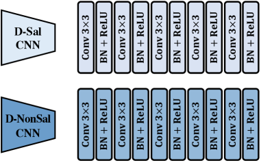
Figure 7: Detailed structure of D-Sal and D-NonSal CNNs in DSU. BN means batch normalization operation.

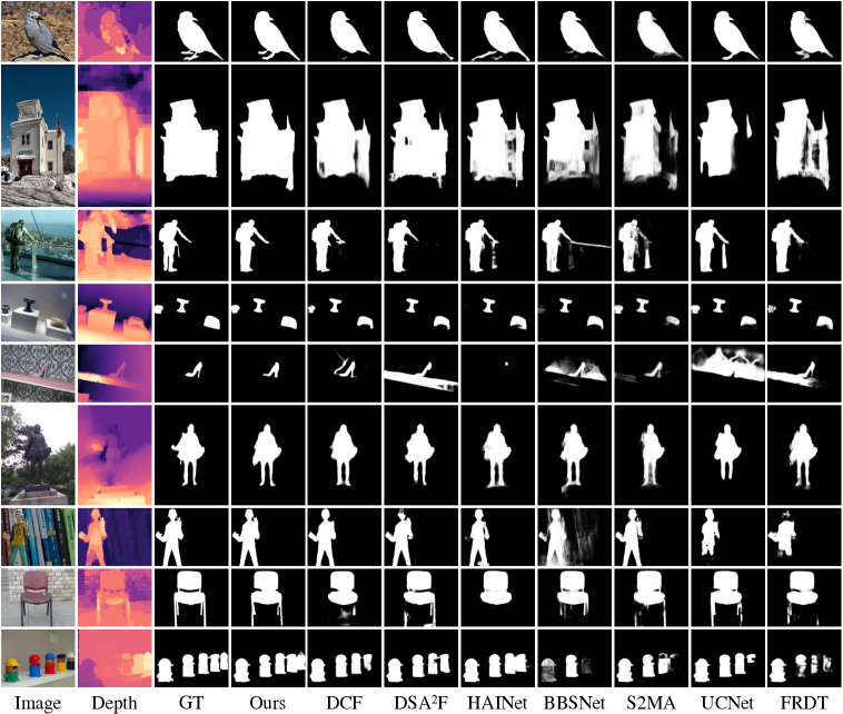
Figure 9: Qualitative comparison of fully-supervised RGB-D SOD methods. Obviously, our fully-supervised variant infers more appealing saliency maps compared to existing SOTA models, including DCF (Ji et al., 2021a). DSA²F (Sun et al., 2021), HAINet (Li et al., 2021a), BBSNet (Fan et al., 2020b), S2MA (Liu et al., 2020), UCNet (Zhang et al., 2020a) and FRDT (Zhang et al., 2020f).

Comparison with current state-of-the-art RGB-D SOD methods under fully-supervised scenario. As discussed in Sec. 4.4 of the main text, our method can boost the performance of existing SOD models greatly, by applying DSU to existing methods. In this section, we further compare our fully-supervised variant of DSU with 25 existing state-of-the-art RGB-D saliency models. We adopt the same feature-extraction backbone (Wu et al., 2019) as in DCF (Ji et al., 2021a) to build the saliency network in the DSU framework. Numerical results in Table 8 and visual results in Fig. 9 consistently show the superiority and scalability of our method.

Pseudo-label Initialization. We investigate other initial pseudo-labels (e.g., DCMC (Cong et al., 2016)), to further verify the effectiveness of our proposed method. The superior performance is also observed, by comparing backbone with ours: 0.167 vs. 0.146 on NJUD, 0.119 vs. 0.084 on NLPR, 0.142 vs. 0.119 on STERE and 0.146 vs. 0.128 on DUTLF-Depth, using MAE metric.

A.3 Implementation Details

The proposed deep unsupervised pipeline is implemented with PyTorch and trained using a single Tesla P40 GPU. Both Saliency and Depth Networks employ the same saliency feature extraction backbone (CPD (Wu et al., 2019)), which is equipped with the encoder of ResNet-50 (He et al., 2016), with initial parameters pre-trained in ImageNet (Krizhevsky et al., 2012). All training & testing images are uniformly resized to the size of $352\times 352$. Throughout training, the learning rate is set to $1\times 10^{-4}$, and the Adam optimizer is used with a mini-batch size of 10. Our approach is trained in an unsupervised manner, i.e., without any human annotations, where initial pseudo-labels are the outputs of handcrafted RGB-D saliency method CDCP (Zhu et al., 2017b). As for the proposed attentive training strategy, its alternation interval is set to 3, amounting to $2\tau=6$ epochs in a training round. During inference, our approach directly predicts saliency maps based on an RGB image, without accessing any depth map.

A.4 Limitation and Discussion

As demonstrated in this paper, our deep unsupervised RGB-D saliency detection approach achieves an appealing trade-off between detection accuracy and human annotation consumption. However, due to the lack of accurate pixel-level annotations, the model still fails to comprehensively detect the fine-grained details, i.e., the edges of salient objects. To tackle this challenge, a doable solution is to introduce auxiliary edge constraint. For example, the edge detection loss can be employed to low-level features of the model, which forces the model to produce discriminative features highlighting object details (Zhang et al., 2020b; Liu et al., 2019). The edge maps can be generated by classical Canny operator (Canny, 1986) in an unsupervised manner. Hopefully this could encourage more inspirations and contributions to this community and further pave the way for its booming future.

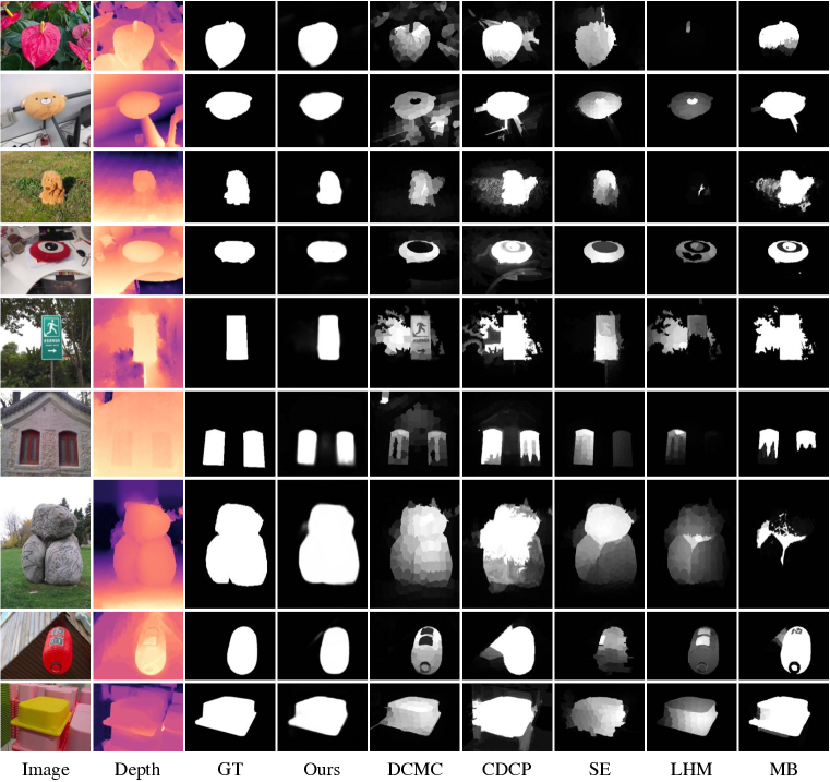
Figure 8: Qualitative comparison with unsupervised RGB-D SOD models. GT means ground-truth.

Table 8: Quantitative results of fully-supervised RGB-D saliency detection methods. The best results are highlighted in boldface. When evaluating the newly released DUTLF-Depth dataset, the specific setup used by (Piao et al., 2019) is adopted to make a fair comparison.

Method	NJUD				NLPR				STERE				DUTLF-Depth
	$E_{\xi}\uparrow$	$F_{\beta}^{w}\uparrow$	$F_{\beta}\uparrow$	$\mathcal{M}\downarrow$	$E_{\xi}\uparrow$	$F_{\beta}^{w}\uparrow$	$F_{\beta}\uparrow$	$\mathcal{M}\downarrow$	$E_{\xi}\uparrow$	$F_{\beta}^{w}\uparrow$	$F_{\beta}\uparrow$	$\mathcal{M}\downarrow$	$E_{\xi}\uparrow$	$F_{\beta}^{w}\uparrow$	$F_{\beta}\uparrow$	$\mathcal{M}\downarrow$
CTMF (Han et al., 2017)	.864	.732	.788	.085	.869	.691	.723	.056	.841	.747	.771	.086	.884	.690	.792	.097
DF (Qu et al., 2017)	.818	.552	.744	.151	.838	.524	.682	.099	.691	.596	.742	.141	.842	.542	.748	.145
PCA (Chen & Li, 2018)	.896	.811	.844	.059	.916	.772	.794	.044	.887	.801	.826	.064	.858	.696	.760	.100
TANet (Chen & Li, 2019)	.893	.812	.844	.061	.916	.789	.795	.041	.893	.804	.835	.060	.866	.712	.779	.093
PDNet (Zhu et al., 2019)	.890	.798	.832	.062	.876	.659	.740	.064	.880	.799	.813	.071	.861	.650	.757	.112
MMCI (Chen et al., 2019)	.878	.749	.813	.079	.871	.688	.729	.059	.873	.757	.829	.068	.855	.636	.753	.113
CPFP (Zhao et al., 2019)	.895	.837	.850	.053	.924	.820	.822	.036	.912	.808	.830	.051	.814	.644	.736	.099
DMRA (Piao et al., 2019)	.908	.853	.872	.051	.942	.845	.855	.031	.923	.841	.876	.049	.927	.858	.883	.048
SSF (Zhang et al., 2020e)	.913	.871	.886	.043	.949	.874	.875	.026	.921	.850	.867	.046	.946	.894	.914	.034
A2dele (Piao et al., 2020)	.897	.851	.874	.051	.945	.867	.878	.028	.915	.855	.874	.044	.924	.864	.890	.043
JL-DCF (Fu et al., 2020)	-	-	-	-	.954	.882	.878	.022	.919	.857	.869	.040	.931	.863	.883	.043
S2MA (Liu et al., 2020)	-	-	-	-	.938	.852	.853	.030	.907	.825	.855	.051	.921	.861	.866	.044
UCNet (Zhang et al., 2020a)	-	-	-	-	.953	.878	.890	.025	.922	.867	.885	.039	.903	.821	.856	.056
FRDT (Zhang et al., 2020f)	.917	.862	.879	.048	.946	.863	.868	.029	.925	.858	.872	.042	.941	.878	.902	.039
D3Net (Fan et al., 2020a)	.913	.860	.863	.047	.943	.854	.857	.030	.920	.845	.855	.046	.847	.668	.756	.097
HDFNet (Pang et al., 2020a)	.915	.879	.893	.038	.948	.869	.878	.027	.925	.863	.879	.040	.934	.865	.892	.040
CMWNet (Li et al., 2020c)	.910	.855	.878	.047	.940	.856	.859	.029	.917	.847	.869	.043	.916	.831	.866	.056
DANet (Zhao et al., 2020c)	-	-	-	-	.949	.858	.871	.028	.914	.830	.858	.047	.925	.847	.884	.047
PGAR (Chen & Fu, 2020)	.915	.871	.893	.042	.955	.881	.885	.024	.919	.856	.880	.041	.944	.889	.914	.035
ATSA (Zhang et al., 2020c)	.921	.883	.893	.040	.945	.867	.876	.028	.919	.866	.874	.040	.947	.901	.918	.032
BBSNet (Fan et al., 2020b)	.924	.884	.902	.035	.952	.879	.882	.023	.925	.858	.885	.041	.833	.663	.774	.120
HAINe (Li et al., 2021a)	.921	.887	.898	.038	.956	.890	.891	.024	.925	.871	.883	.040	.938	.883	.906	.038
RD3D (Chen et al., 2021b)	.918	.889	.900	.037	.956	.894	.890	.022	.926	.877	.885	.038	.949	.908	.914	.031
DSA2F (Sun et al., 2021)	.923	.889	.901	.039	.950	.889	.897	.024	.927	.877	.895	.038	.949	.908	.924	.032
DCF (Ji et al., 2021a)	.924	.893	.902	.035	.957	.892	.891	.021	.927	.873	.885	.039	.952	.909	.926	.030
Ours (fully supervised)	.926	.894	.909	.036	.957	.897	.907	.022	.927	.882	.895	.037	.951	.911	.918	.031

A.5 Additional Analysis

In this paper, our DSU design achieves appealing trade-off between model performance and complexity since our method has additional benefits of not introducing extra test-time cost and not relying on the depth map during the inference stage, as shown in Table 1 and Fig. 1. Meanwhile, our method can be easily adapted to integrate useful depth cues by engaging the proposed DSU and DLU. In Table 9, we conduct an interesting experiment, comparing the model performance, inference speed, FLOPs and parameter number, when using only RGB stream versus using RGB and depth simultaneously during inference. It is observed that introducing depth information can further improve the model performance, but at the same time, it will lead to the decrease of inference speed, and the increases of FLOPs and parameters. These results further demonstrate the effectiveness and efficiency of our DSU design.

Table 9: Quantitative results of our DSU when using only RGB stream versus using RGB and depth simultaneously during inference.

	Model Complexity			Model Performance (NLPR)
	Speed$\uparrow$	FLOPs$\downarrow$	Parameters$\downarrow$	$E_{\xi}$$\uparrow$	$F_{\beta}^{w}$$\uparrow$	$F_{\beta}$$\uparrow$	$\mathcal{M}$$\downarrow$
Our lightweight design (only using RGB)	35 FPS	17.87 G	47.85 MB	0.879	0.657	0.745	0.065
with additional depth (using RGB and depth)	21 FPS	45.16 G	96.53 MB	0.885	0.670	0.762	0.062

A.6 Future Direction

In this paper, we make the earliest effort to explore deep unsupervised learning in RGB-D SOD, which is demonstrated to achieve appealing performance without involving any human annotations during training. To our best knowledge, this is the first such attempt in RGB-D SOD. Meanwhile, we also investigate several potential directions for future research as follows.

(1) Exploring on the utilization of depth. The lack of explicit pixel-level supervision brings new challenge to the RGB-D SOD task, that is, inconsistency and large variations in raw depth maps. In this paper, we address it from two aspects. For depth variations between salient objects and background (i.e., possible inter-class variance), a depth-disentangled network is designed to learn the discriminative saliency cues and non-salient background from raw depth map. For variance within salient objects (i.e., possible intra-object variance), we use thresholding and normalization operations to remove illegal numbers, and apply CRF to smooth the updated pseudo-labels in DLU. One promising future direction is that we can include some post-processing operations to make highlighted region on the “depth-revealed saliency map” uniform before using it to update pseudo-labels. Here we provide an extended experiment in Table 10, where we smooth the inconsistent depth using a new CRF before feeding it to the DLU. This results in higher performance benefiting from more uniform depth. We believe more dedicated algorithm is worth exploring in future work to deal with inconsistent depth.

Table 10: Ablated experiment on the utilization of depth.

	NLPR				NJUD
	$E_{\xi}$$\uparrow$	$F_{\beta}^{w}$$\uparrow$	$F_{\beta}$$\uparrow$	$\mathcal{M}$$\downarrow$	$E_{\xi}$$\uparrow$	$F_{\beta}^{w}$$\uparrow$	$F_{\beta}$$\uparrow$	$\mathcal{M}$$\downarrow$
Our DSU framework	0.879	0.657	0.745	0.065	0.797	0.597	0.719	0.135
Our DSU using saliency-guided depth with CRF	0.885	0.661	0.751	0.064	0.799	0.603	0.724	0.133

(2) Exploring on alleviating noise in unsupervised learning. Noisy problem has always been a universal and inevitable problem for unsupervised learning. In this paper, the proposed ATS strategy is able to alleviate this problem by properly re-weighting to reduce the influence of the ambiguous pseudo-label during training. One promising future direction is that we can design new algorithms to model the uncertainty regions and train the saliency network with partial BCE loss to alleviate the noisy issue of pseudo-labels.

(3) Exploring on generating high-quality pseudo-labels. In our paper, a depth-disentangled saliency update (DSU) framework is designed to automatically produce pseudo-labels with iterative follow-up refinements, which is able to provide more trustworthy supervision signals for training the saliency network. For future work, we can explore other algorithms to generate high-quality pseudo-labels, for example, 1) imposing contrastive loss (e.g., using superpixel candidates with ROI pooling to construct contrastive pairs) to enlarge the feature distance between foreground and background; 2) involving partially labeled scribbles to help generate more accurate pseudo-labels.

(4) Exploring on more fine-grained disentangled framework. In this paper, we design a depth-disentangled saliency update framework to decompose depth information into saliency-guided and non-saliency-guided depths to promote saliency, motivated by the nature of the class-agnostic binary salient object segmentation task. It is worthy exploring in the future to design more fine-grained disentangled framework. For example, in addition to the saliency-guided depth and non-saliency-guided depth, we can additionally model the ‘not sure’ regions by learning an uncertainty map (using well-designed new algorithms such as Monte Carlo Dropout (Gal & Ghahramani, 2016)). The learned uncertainty map, which reveals the ‘not sure’ regions, can engage in the pseudo-label training process to mitigate the noises of uncertain pseudo-labels, using partial BCE loss.

(5) Exploring on more applications. SOD is useful for a variety of downstream applications including image classification (Chen et al., 2021c; Bi et al., 2021; Ning et al., 2021a; c), light-field data (Zhang et al., 2019; 2020d), medical image processing (Zhao et al., 2021b; Ji et al., 2021b; 2020a; Yao et al., 2021b; a; Ning et al., 2021b; 2020), and video analysis (Zhang et al., 2021; Zhao et al., 2021a), etc. This is benefiting from its generic mechanism to highlight class-agnostic objects in a scene. For unsupervised RGB-D SOD, it can be regarded as a pre-task or prior to effectively improve the performance of target task (e.g., weakly supervised semantic segmentation, action recognization), and avoid more laborious efforts.

As discussed above, we summarize five potential research directions for deep unsupervised RGB-D salient object detection. Hopefully this could encourage more inspirations and contributions to this community.

References

- Achanta et al. (2009) Radhakrishna Achanta, Sheila Hemami, Francisco Estrada, and Sabine Susstrunk. Frequency-tuned salient region detection. In Proceedings of the IEEE Conference on Computer Vision and Pattern Recognition, pp. 1597–1604, 2009.
- Bi et al. (2021) Qi Bi, Shuang Yu, Wei Ji, Cheng Bian, Lijun Gong, Hanruo Liu, Kai Ma, and Yefeng Zheng. Local-global dual perception based deep multiple instance learning for retinal disease classification. In International Conference on Medical Image Computing and Computer-Assisted Intervention, pp. 55–64. Springer, 2021.
- Borji et al. (2015) Ali Borji, Ming-Ming Cheng, Huaizu Jiang, and Jia Li. Salient object detection: A benchmark. IEEE Transactions on Image Processing, 24(12):5706–5722, 2015.
- Canny (1986) John Canny. A computational approach to edge detection. IEEE Transactions on Pattern Analysis and Machine Intelligence, 8(6):679–698, 1986.
- Chen et al. (2020a) Chenglizhao Chen, Jipeng Wei, Chong Peng, Weizhong Zhang, and Hong Qin. Improved saliency detection in RGB-D images using two-phase depth estimation and selective deep fusion. IEEE Transactions on Image Processing, 29:4296–4307, 2020a.
- Chen et al. (2021a) Chenglizhao Chen, Jipeng Wei, Chong Peng, and Hong Qin. Depth-quality-aware salient object detection. IEEE Transactions on Image Processing, 30:2350–2363, 2021a.
- Chen & Li (2018) Hao Chen and Youfu Li. Progressively complementarity-aware fusion network for RGB-D salient object detection. In Proceedings of the IEEE Conference on Computer Vision and Pattern Recognition, pp. 3051–3060, 2018.
- Chen & Li (2019) Hao Chen and Youfu Li. Three-stream attention-aware network for RGB-D salient object detection. IEEE Transactions on Image Processing, 28(6):2825–2835, 2019.
- Chen et al. (2019) Hao Chen, Youfu Li, and Dan Su. Multi-modal fusion network with multi-scale multi-path and cross-modal interactions for RGB-D salient object detection. Pattern Recognition, 86:376–385, 2019.
- Chen et al. (2021b) Qian Chen, Ze Liu, Yi Zhang, Keren Fu, Qijun Zhao, and Hongwei Du. RGB-D salient object detection via 3D convolutional neural. In The Thirty-Fifth AAAI Conference on Artificial Intelligence, 2021b.
- Chen & Fu (2020) Shuhan Chen and Yun Fu. Progressively guided alternate refinement network for RGB-D salient object detection. In Proceedings of the European Conference on Computer Vision, 2020.
- Chen et al. (2021c) Wenting Chen, Shuang Yu, Kai Ma, Wei Ji, Cheng Bian, Chunyan Chu, Linlin Shen, and Yefeng Zheng. Tw-gan: Topology and width aware gan for retinal artery/vein classification. Medical Image Analysis, pp. 102340, 2021c.
- Chen et al. (2020b) Zuyao Chen, Runmin Cong, Qianqian Xu, and Qingming Huang. DPANet: Depth potentiality-aware gated attention network for RGB-D salient object detection. IEEE Transactions on Image Processing, 2020b.
- Cheng et al. (2014) Yupeng Cheng, Huazhu Fu, Xingxing Wei, Jiangjian Xiao, and Xiaochun Cao. Depth enhanced saliency detection method. In Proceedings of International Conference on Internet Multimedia Computing and Service, pp. 23–27, 2014.
- Cong et al. (2016) Runmin Cong, Jianjun Lei, Changqing Zhang, Qingming Huang, Xiaochun Cao, and Chunping Hou. Saliency detection for stereoscopic images based on depth confidence analysis and multiple cues fusion. IEEE Signal Processing Letters, 23(6):819–823, 2016.
- Desingh et al. (2013) Karthik Desingh, K Madhava Krishna, Deepu Rajan, and CV Jawahar. Depth really matters: Improving visual salient region detection with depth. In British Machine Vision Conference, 2013.
- Dixon (1999) Nancy M Dixon. The organizational learning cycle: How we can learn collectively. Gower Publishing, Ltd., 1999.
- Fan et al. (2018) Deng-Ping Fan, Cheng Gong, Yang Cao, Bo Ren, Ming-Ming Cheng, and Ali Borji. Enhanced-alignment measure for binary foreground map evaluation. In Proceedings of the 27th International Joint Conference on Artificial Intelligence, pp. 698–704, 2018.
- Fan et al. (2020a) Deng-Ping Fan, Zheng Lin, Zhao Zhang, Menglong Zhu, and Ming-Ming Cheng. Rethinking RGB-D salient object detection: Models, data sets, and large-scale benchmarks. IEEE Transactions on Neural Networks and Learning Systems, 2020a.
- Fan et al. (2020b) Deng-Ping Fan, Yingjie Zhai, Ali Borji, Jufeng Yang, and Ling Shao. BBS-Net: RGB-D salient object detection with a bifurcated backbone strategy network. In Proceedings of the European Conference on Computer Vision, 2020b.
- Feng et al. (2016) David Feng, Nick Barnes, Shaodi You, and Chris McCarthy. Local background enclosure for RGB-D salient object detection. In Proceedings of the IEEE Conference on Computer Vision and Pattern Recognition, pp. 2343–2350, 2016.
- Fu et al. (2020) Keren Fu, Deng-Ping Fan, Ge-Peng Ji, and Qijun Zhao. JL-DCF: Joint learning and densely-cooperative fusion framework for RGB-D salient object detection. In Proceedings of the IEEE Conference on Computer Vision and Pattern Recognition, pp. 3052–3062, 2020.
- Gal & Ghahramani (2016) Yarin Gal and Zoubin Ghahramani. Dropout as a Bayesian approximation: Representing model uncertainty in deep learning. In International Conference on Machine Learning, pp. 1050–1059, 2016.
- Giancola et al. (2018) Silvio Giancola, Matteo Valenti, and Remo Sala. A Survey on 3D Cameras: Metrological Comparison of Time-of-Flight, Structured-Light and Active Stereoscopy Technologies. Springer, 2018.
- Guo et al. (2016) Jingfan Guo, Tongwei Ren, and Jia Bei. Salient object detection for RGB-D image via saliency evolution. In IEEE International Conference on Multimedia and Expo, pp. 1–6, 2016.
- Han et al. (2017) Junwei Han, Hao Chen, Nian Liu, Chenggang Yan, and Xuelong Li. CNNs-based RGB-D saliency detection via cross-view transfer and multiview fusion. IEEE Transactions on Cybernetics, 48(11):3171–3183, 2017.
- He et al. (2016) Kaiming He, Xiangyu Zhang, Shaoqing Ren, and Jian Sun. Deep residual learning for image recognition. In Proceedings of the IEEE Conference on Computer Vision and Pattern Recognition, pp. 770–778, 2016.
- Hou et al. (2017) Qibin Hou, Ming-Ming Cheng, Xiaowei Hu, Ali Borji, Zhuowen Tu, and Philip HS Torr. Deeply supervised salient object detection with short connections. In Proceedings of the IEEE Conference on Computer Vision and Pattern Recognition, pp. 3203–3212, 2017.
- Hsu et al. (2018a) Kuang-Jui Hsu, Yen-Yu Lin, Yung-Yu Chuang, et al. Co-attention cnns for unsupervised object co-segmentation. In IJCAI, pp. 748–756, 2018a.
- Hsu et al. (2018b) Kuang-Jui Hsu, Chung-Chi Tsai, Yen-Yu Lin, Xiaoning Qian, and Yung-Yu Chuang. Unsupervised cnn-based co-saliency detection with graphical optimization. In European Conference on Computer Vision, pp. 485–501, 2018b.
- Ji et al. (2020a) Wei Ji, Wenting Chen, Shuang Yu, Kai Ma, Li Cheng, Linlin Shen, and Yefeng Zheng. Uncertainty quantification for medical image segmentation using dynamic label factor allocation among multiple raters. In MICCAI on QUBIQ Workshop, 2020a.
- Ji et al. (2020b) Wei Ji, Jingjing Li, Miao Zhang, Yongri Piao, and Huchuan Lu. Accurate RGB-D salient object detection via collaborative learning. In Proceedings of the European Conference on Computer Vision, pp. 52–69, 2020b.
- Ji et al. (2021a) Wei Ji, Jingjing Li, Shuang Yu, Miao Zhang, Yongri Piao, Shunyu Yao, Qi Bi, Kai Ma, Yefeng Zheng, Huchuan Lu, and Li Cheng. Calibrated rgb-d salient object detection. In Proceedings of the IEEE Conference on Computer Vision and Pattern Recognition, pp. 9471–9481, 2021a.
- Ji et al. (2021b) Wei Ji, Shuang Yu, Junde Wu, Kai Ma, Cheng Bian, Qi Bi, Jingjing Li, Hanruo Liu, Li Cheng, and Yefeng Zheng. Learning calibrated medical image segmentation via multi-rater agreement modeling. In Proceedings of the IEEE Conference on Computer Vision and Pattern Recognition, pp. 12341–12351, 2021b.
- Ji et al. (2022) Wei Ji, Ge Yan, Jingjing Li, Yongri Piao, Shunyu Yao, Miao Zhang, Li Cheng, and Huchuan Lu. Dmra: Depth-induced multi-scale recurrent attention network for rgb-d saliency detection. IEEE Transactions on Image Processing, 31:2321–2336, 2022.
- Ju et al. (2014) Ran Ju, Ling Ge, Wenjing Geng, Tongwei Ren, and Gangshan Wu. Depth saliency based on anisotropic center-surround difference. In IEEE International Conference on Image Processing, pp. 1115–1119, 2014.
- Ko et al. (2004) ByoungChul Ko, Soo Yeong Kwak, and Hyeran Byun. SVM-based salient region(s) extraction method for image retrieval. In Proceedings of the 17th International Conference on Pattern Recognition, volume 2, pp. 977–980, 2004.
- Krizhevsky et al. (2012) Alex Krizhevsky, Ilya Sutskever, and Geoffrey E Hinton. ImageNet classification with deep convolutional neural networks. In Advances in Neural Information Processing Systems, pp. 1097–1105, 2012.
- Li et al. (2020a) Chongyi Li, Runmin Cong, Sam Kwong, Junhui Hou, Huazhu Fu, Guopu Zhu, Dingwen Zhang, and Qingming Huang. ASIF-Net: Attention steered interweave fusion network for RGB-D salient object detection. IEEE Transactions on Cybernetics, PP(99):1–13, 2020a.
- Li et al. (2020b) Chongyi Li, Runmin Cong, Yongri Piao, Qianqian Xu, and Chen Change Loy. RGB-D salient object detection with cross-modality modulation and selection. In Proceedings of the European Conference on Computer Vision, 2020b.
- Li et al. (2020c) Gongyang Li, Zhi Liu, Linwei Ye, Yang Wang, and Haibin Ling. Cross-modal weighting network for RGB-D salient object detection. In Proceedings of the European Conference on Computer Vision, 2020c.
- Li et al. (2021a) Gongyang Li, Zhi Liu, Minyu Chen, Zhen Bai, Weisi Lin, and Haibin Ling. Hierarchical alternate interaction network for RGB-D salient object detection. IEEE Transactions on Image Processing, 2021a.
- Li et al. (2021b) Jingjing Li, Wei Ji, Qi Bi, Cheng Yan, Miao Zhang, Yongri Piao, Huchuan Lu, et al. Joint semantic mining for weakly supervised rgb-d salient object detection. Advances in Neural Information Processing Systems, 34:11945–11959, 2021b.
- Li et al. (2013) Xiaohui Li, Huchuan Lu, Lihe Zhang, Xiang Ruan, and Ming-Hsuan Yang. Saliency detection via dense and sparse reconstruction. In Proceedings of the IEEE International Conference on Computer Vision, pp. 2976–2983, 2013.
- Liang et al. (2018) Fangfang Liang, Lijuan Duan, Wei Ma, Yuanhua Qiao, Zhi Cai, and Laiyun Qing. Stereoscopic saliency model using contrast and depth-guided-background prior. Neurocomputing, 275:2227–2238, 2018.
- Liao et al. (2020) Guibiao Liao, Wei Gao, Qiuping Jiang, Ronggang Wang, and Ge Li. MMNet: Multi-stage and multi-scale fusion network for RGB-D salient object detection. In Proceedings of the 28th ACM International Conference on Multimedia, pp. 2436–2444, 2020.
- Liu et al. (2008) Huiying Liu, Shuqiang Jiang, Qingming Huang, and Changsheng Xu. A generic virtual content insertion system based on visual attention analysis. In Proceedings of the 16th ACM International Conference on Multimedia, pp. 379–388, 2008.
- Liu et al. (2019) Jiang-Jiang Liu, Qibin Hou, Ming-Ming Cheng, Jiashi Feng, and Jianmin Jiang. A simple pooling-based design for real-time salient object detection. In Proceedings of the IEEE Conference on Computer Vision and Pattern Recognition, pp. 3917–3926, 2019.
- Liu et al. (2018) Nian Liu, Junwei Han, and Ming-Hsuan Yang. Picanet: Learning pixel-wise contextual attention for saliency detection. In Proceedings of the IEEE Conference on Computer Vision and Pattern Recognition, pp. 3089–3098, 2018.
- Liu et al. (2020) Nian Liu, Ni Zhang, and Junwei Han. Learning selective self-mutual attention for RGB-D saliency detection. In Proceedings of the IEEE Conference on Computer Vision and Pattern Recognition, pp. 13756–13765, 2020.
- Luo et al. (2020) Ao Luo, Xin Li, Fan Yang, Zhicheng Jiao, Hong Cheng, and Siwei Lyu. Cascade graph neural networks for RGB-D salient object detection. In Proceedings of the European Conference on Computer Vision, 2020.
- Ma et al. (2021) Mingcan Ma, Changqun Xia, and Jia Li. Pyramidal feature shrinking for salient object detection. In Proceedings of the AAAI Conference on Artificial Intelligence, pp. 2311–2318, 2021.
- Margolin et al. (2014) Ran Margolin, Lihi Zelnik-Manor, and Ayellet Tal. How to evaluate foreground maps? In Proceedings of the IEEE Conference on Computer Vision and Pattern Recognition, pp. 248–255, 2014.
- Nguyen et al. (2019) Tam Nguyen, Maximilian Dax, Chaithanya Kumar Mummadi, Nhung Ngo, Thi Hoai Phuong Nguyen, Zhongyu Lou, and Thomas Brox. DeepUSPS: Deep robust unsupervised saliency prediction via self-supervision. In Advances in Neural Information Processing Systems, pp. 204–214, 2019.
- Ning et al. (2020) Munan Ning, Cheng Bian, Donghuan Lu, Hong-Yu Zhou, Shuang Yu, Chenglang Yuan, Yang Guo, Yaohua Wang, Kai Ma, and Yefeng Zheng. A macro-micro weakly-supervised framework for as-oct tissue segmentation. In International Conference on Medical Image Computing and Computer-Assisted Intervention, pp. 725–734. Springer, 2020.
- Ning et al. (2021a) Munan Ning, Cheng Bian, Dong Wei, Shuang Yu, Chenglang Yuan, Yaohua Wang, Yang Guo, Kai Ma, and Yefeng Zheng. A new bidirectional unsupervised domain adaptation segmentation framework. In International Conference on Information Processing in Medical Imaging, pp. 492–503. Springer, 2021a.
- Ning et al. (2021b) Munan Ning, Cheng Bian, Chenglang Yuan, Kai Ma, and Yefeng Zheng. Ensembled resunet for anatomical brain barriers segmentation. Segmentation, Classification, and Registration of Multi-modality Medical Imaging Data, 12587:27, 2021b.
- Ning et al. (2021c) Munan Ning, Donghuan Lu, Dong Wei, Cheng Bian, Chenglang Yuan, Shuang Yu, Kai Ma, and Yefeng Zheng. Multi-anchor active domain adaptation for semantic segmentation. In Proceedings of the IEEE International Conference on Computer Vision, 2021c.
- Niu et al. (2012) Yuzhen Niu, Yujie Geng, Xueqing Li, and Feng Liu. Leveraging stereopsis for saliency analysis. In Proceedings of the IEEE Conference on Computer Vision and Pattern Recognition, pp. 454–461, 2012.
- Otsu (1979) Nobuyuki Otsu. A threshold selection method from gray-level histograms. IEEE Transactions on Systems, Man, and Cybernetics, 9(1):62–66, 1979.
- Pang et al. (2020a) Youwei Pang, Lihe Zhang, Xiaoqi Zhao, and Huchuan Lu. Hierarchical dynamic filtering network for RGB-D salient object detection. In Proceedings of the European Conference on Computer Vision, 2020a.
- Pang et al. (2020b) Youwei Pang, Xiaoqi Zhao, Lihe Zhang, and Huchuan Lu. Multi-scale interactive network for salient object detection. In Proceedings of the IEEE Conference on Computer Vision and Pattern Recognition, pp. 9413–9422, 2020b.
- Peltier et al. (2005) James W Peltier, Amanda Hay, and William Drago. The reflective learning continuum: Reflecting on reflection. Journal of marketing education, 27(3):250–263, 2005.
- Peng et al. (2014) Houwen Peng, Bing Li, Weihua Xiong, Weiming Hu, and Rongrong Ji. RGBD salient object detection: a benchmark and algorithms. In Proceedings of the European Conference on Computer Vision, pp. 92–109, 2014.
- Piao et al. (2019) Yongri Piao, Wei Ji, Jingjing Li, Miao Zhang, and Huchuan Lu. Depth-induced multi-scale recurrent attention network for saliency detection. In Proceedings of the IEEE International Conference on Computer Vision, pp. 7254–7263, 2019.
- Piao et al. (2020) Yongri Piao, Zhengkun Rong, Miao Zhang, Weisong Ren, and Huchuan Lu. A2dele: Adaptive and attentive depth distiller for efficient RGB-D salient object detection. In Proceedings of the IEEE Conference on Computer Vision and Pattern Recognition, pp. 9060–9069, 2020.
- Qin et al. (2015) Yao Qin, Huchuan Lu, Yiqun Xu, and He Wang. Saliency detection via cellular automata. In Proceedings of the IEEE Conference on Computer Vision and Pattern Recognition, pp. 110–119, 2015.
- Qu et al. (2017) Liangqiong Qu, Shengfeng He, Jiawei Zhang, Jiandong Tian, Yandong Tang, and Qingxiong Yang. RGBD salient object detection via deep fusion. IEEE Transactions on Image Processing, 26(5):2274–2285, 2017.
- Ren et al. (2015) Jianqiang Ren, Xiaojin Gong, Lu Yu, Wenhui Zhou, and Michael Ying Yang. Exploiting global priors for RGB-D saliency detection. In Proceedings of the IEEE Conference on Computer Vision and Pattern Recognition Workshops, pp. 25–32, 2015.
- Shao & Brady (2006) Ling Shao and Michael Brady. Specific object retrieval based on salient regions. Pattern Recognition, 39(10):1932–1948, 2006.
- Shigematsu et al. (2017) Riku Shigematsu, David Feng, Shaodi You, and Nick Barnes. Learning RGB-D salient object detection using background enclosure, depth contrast, and top-down features. In Proceedings of the IEEE International Conference on Computer Vision Workshops, pp. 2749–2757, 2017.
- Simonyan & Zisserman (2015) Karen Simonyan and Andrew Zisserman. Very deep convolutional networks for large-scale image recognition. In International Conference on Learning Representations, 2015.
- Sun et al. (2021) Peng Sun, Wenhu Zhang, Huanyu Wang, Songyuan Li, and Xi Li. Deep RGB-D saliency detection with depth-sensitive attention and automatic multi-modal fusion. In Proceedings of the IEEE Conference on Computer Vision and Pattern Recognition, pp. 1407–1417, 2021.
- Tsai et al. (2018) Chung-Chi Tsai, Weizhi Li, Kuang-Jui Hsu, Xiaoning Qian, and Yen-Yu Lin. Image co-saliency detection and co-segmentation via progressive joint optimization. IEEE Transactions on Image Processing, 28(1):56–71, 2018.
- Tsai et al. (2019) Chung-Chi Tsai, Kuang-Jui Hsu, Yen-Yu Lin, Xiaoning Qian, and Yung-Yu Chuang. Deep co-saliency detection via stacked autoencoder-enabled fusion and self-trained cnns. IEEE Transactions on Multimedia, 22(4):1016–1031, 2019.
- Tu et al. (2016) Wei-Chih Tu, Shengfeng He, Qingxiong Yang, and Shao-Yi Chien. Real-time salient object detection with a minimum spanning tree. In Proceedings of the IEEE Conference on Computer Vision and Pattern Recognition, pp. 2334–2342, 2016.
- Wang et al. (2018) Wenguan Wang, Jianbing Shen, Fang Guo, Ming-Ming Cheng, and Ali Borji. Revisiting video saliency: A large-scale benchmark and a new model. In Proceedings of the IEEE Conference on Computer Vision and Pattern Recognition, pp. 4894–4903, 2018.
- Wang et al. (2021) Wenguan Wang, Qiuxia Lai, Huazhu Fu, Jianbing Shen, Haibin Ling, and Ruigang Yang. Salient object detection in the deep learning era: An in-depth survey. IEEE Transactions on Pattern Analysis and Machine Intelligence, 2021.
- Wu et al. (2019) Zhe Wu, Li Su, and Qingming Huang. Cascaded partial decoder for fast and accurate salient object detection. In Proceedings of the IEEE Conference on Computer Vision and Pattern Recognition, pp. 3907–3916, 2019.
- Xu et al. (2021) Binwei Xu, Haoran Liang, Ronghua Liang, and Peng Chen. Locate globally, segment locally: A progressive architecture with knowledge review network for salient object detection. In Proceedings of the AAAI Conference on Artificial Intelligence, pp. 3004–3012, 2021.
- Xu et al. (2015) Kelvin Xu, Jimmy Ba, Ryan Kiros, Kyunghyun Cho, Aaron Courville, Ruslan Salakhudinov, Rich Zemel, and Yoshua Bengio. Show, attend and tell: Neural image caption generation with visual attention. In International Conference on Machine Learning, pp. 2048–2057, 2015.
- Yao et al. (2021a) Qingsong Yao, Quan Quan, Li Xiao, and S Kevin Zhou. One-shot medical landmark detection. arXiv preprint arXiv:2103.04527, 2021a.
- Yao et al. (2021b) Qingsong Yao, Li Xiao, Peihang Liu, and S Kevin Zhou. Label-free segmentation of covid-19 lesions in lung ct. IEEE Transactions on Medical Imaging, 2021b.
- Zhang et al. (2017) Dingwen Zhang, Junwei Han, and Yu Zhang. Supervision by fusion: Towards unsupervised learning of deep salient object detector. In Proceedings of the IEEE International Conference on Computer Vision, pp. 4048–4056, 2017.
- Zhang et al. (2018) Jing Zhang, Tong Zhang, Yuchao Dai, Mehrtash Harandi, and Richard Hartley. Deep unsupervised saliency detection: A multiple noisy labeling perspective. In Proceedings of the IEEE Conference on Computer Vision and Pattern Recognition, pp. 9029–9038, 2018.
- Zhang et al. (2020a) Jing Zhang, Deng-Ping Fan, Yuchao Dai, Saeed Anwar, Fatemeh Sadat Saleh, Tong Zhang, and Nick Barnes. UC-Net: Uncertainty inspired RGB-D saliency detection via conditional variational autoencoders. In Proceedings of the IEEE Conference on Computer Vision and Pattern Recognition, pp. 8582–8591, 2020a.
- Zhang et al. (2020b) Jing Zhang, Xin Yu, Aixuan Li, Peipei Song, Bowen Liu, and Yuchao Dai. Weakly-supervised salient object detection via scribble annotations. In Proceedings of the IEEE Conference on Computer Vision and Pattern Recognition, pp. 12546–12555, 2020b.
- Zhang et al. (2019) Miao Zhang, Jingjing Li, Wei Ji, Yongri Piao, and Huchuan Lu. Memory-oriented decoder for light field salient object detection. In Advances in Neural Information Processing Systems, pp. 898–908, 2019.
- Zhang et al. (2020c) Miao Zhang, Sun Xiao Fei, Jie Liu, Shuang Xu, Yongri Piao, and Huchuan Lu. Asymmetric two-stream architecture for accurate RGB-D saliency detection. In Proceedings of the European Conference on Computer Vision, 2020c.
- Zhang et al. (2020d) Miao Zhang, Wei Ji, Yongri Piao, Jingjing Li, Yu Zhang, Shuang Xu, and Huchuan Lu. Lfnet: Light field fusion network for salient object detection. IEEE Transactions on Image Processing, 29:6276–6287, 2020d.
- Zhang et al. (2020e) Miao Zhang, Weisong Ren, Yongri Piao, Zhengkun Rong, and Huchuan Lu. Select, supplement and focus for RGB-D saliency detection. In Proceedings of the IEEE Conference on Computer Vision and Pattern Recognition, pp. 3472–3481, 2020e.
- Zhang et al. (2020f) Miao Zhang, Yu Zhang, Yongri Piao, Beiqi Hu, and Huchuan Lu. Feature reintegration over differential treatment: A top-down and adaptive fusion network for RGB-D salient object detection. In ACM International Conference on Multimedia, 2020f.
- Zhang et al. (2021) Miao Zhang, Jie Liu, Yifei Wang, Yongri Piao, Shunyu Yao, Wei Ji, Jingjing Li, Huchuan Lu, and Zhongxuan Luo. Dynamic context-sensitive filtering network for video salient object detection. In Proceedings of the IEEE International Conference on Computer Vision, pp. 1553–1563, 2021.
- Zhao et al. (2019) Jia-Xing Zhao, Yang Cao, Deng-Ping Fan, Ming-Ming Cheng, Xuan-Yi Li, and Le Zhang. Contrast prior and fluid pyramid integration for RGBD salient object detection. In Proceedings of the IEEE Conference on Computer Vision and Pattern Recognition, pp. 3927–3936, 2019.
- Zhao et al. (2020a) Jiawei Zhao, Yifan Zhao, Jia Li, and Xiaowu Chen. Is depth really necessary for salient object detection? In ACM International Conference on Multimedia, 2020a.
- Zhao et al. (2020b) Xiaoqi Zhao, Youwei Pang, Lihe Zhang, Huchuan Lu, and Lei Zhang. Suppress and balance: A simple gated network for salient object detection. In Proceedings of the European Conference on Computer Vision, 2020b.
- Zhao et al. (2020c) Xiaoqi Zhao, Lihe Zhang, Youwei Pang, Huchuan Lu, and Lei Zhang. A single stream network for robust and real-time RGB-D salient object detection. In Proceedings of the European Conference on Computer Vision, 2020c.
- Zhao et al. (2021a) Xiaoqi Zhao, Youwei Pang, Jiaxing Yang, Lihe Zhang, and Huchuan Lu. Multi-source fusion and automatic predictor selection for zero-shot video object segmentation. In ACM International Conference on Multimedia, pp. 2645–2653, 2021a.
- Zhao et al. (2021b) Xiaoqi Zhao, Lihe Zhang, and Huchuan Lu. Automatic polyp segmentation via multi-scale subtraction network. In International Conference on Medical Image Computing and Computer-Assisted Intervention. Springer, 2021b.
- Zhao et al. (2022) Xiaoqi Zhao, Youwei Pang, Lihe Zhang, Huchuan Lu, and Xiang Ruan. Self-supervised pretraining for rgb-d salient object detection. In Proceedings of the AAAI Conference on Artificial Intelligence, 2022.
- Zhou et al. (2021) Tao Zhou, Deng-Ping Fan, Ming-Ming Cheng, Jianbing Shen, and Ling Shao. RGB-D salient object detection: A survey. Computational visual media, pp. 1–33, 2021.
- Zhu et al. (2017a) Chunbiao Zhu, Ge Li, Xiaoqiang Guo, Wenmin Wang, and Ronggang Wang. A multilayer backpropagation saliency detection algorithm based on depth mining. In International Conference on Computer Analysis of Images and Patterns, pp. 14–23, 2017a.
- Zhu et al. (2017b) Chunbiao Zhu, Ge Li, Wenmin Wang, and Ronggang Wang. An innovative salient object detection using center-dark channel prior. In Proceedings of the IEEE International Conference on Computer Vision Workshops, pp. 1509–1515, 2017b.
- Zhu et al. (2019) Chunbiao Zhu, Xing Cai, Kan Huang, Thomas H Li, and Ge Li. PDNet: Prior-model guided depth-enhanced network for salient object detection. In IEEE International Conference on Multimedia and Expo, pp. 199–204, 2019.
- Zhu et al. (2014) Wangjiang Zhu, Shuang Liang, Yichen Wei, and Jian Sun. Saliency optimization from robust background detection. In Proceedings of the IEEE Conference on Computer Vision and Pattern Recognition, pp. 2814–2821, 2014.