Sparsity-Aware Robust Normalized Subband Adaptive Filtering algorithms based on Alternating Optimization

Abstract

This paper proposes a unified sparsity-aware robust normalized subband adaptive filtering (SA-RNSAF) algorithm for identification of sparse systems under impulsive noise. The proposed SA-RNSAF algorithm generalizes different algorithms by defining the robust criterion and sparsity-aware penalty. Furthermore, by alternating optimization of the parameters (AOP) of the algorithm, including the step-size and the sparsity penalty weight, we develop the AOP-SA-RNSAF algorithm, which not only exhibits fast convergence but also obtains low steady-state misadjustment for sparse systems. Simulations in various noise scenarios have verified that the proposed AOP-SA-RNSAF algorithm outperforms existing techniques.

I Introduction

For highly correlated input signals, the normalized subband adaptive filtering (NSAF) [1] algorithm provides faster convergence than the normalized least mean square (NLMS) algorithm and retains comparable complexity. The NSAF algorithm was proposed based on the multiband structure of subband filters [2], which adjusts the fullband filter’s coefficients to remove the aliasing and band edge effects of the conventional subband structure [2]. However, in practice the non-Gaussian noise with impulsive samples could commonly happen such as in echo cancellation, underwater acoustics, audio processing, and communications [3, 4], and in this scenario, the NSAF performance degrades. To deal with impulsive noises, several robust subband algorithms based on different robust criteria were proposed, see [5, 6, 7, 8, 9, 10] and references therein, and most of them can be unified as the NSAF update with a specific scaling factor.

Furthermore, it is interesting to improve the adaptive filter performance by exploiting the system sparsity. For example, the impulse responses of propagation channels in underwater acoustic and radio communications are usually sparse [11, 12], only a few coefficients of which are non-zero. Aiming at sparse systems, existing examples are classified into the proportionate type and sparsity-aware type. The family of proportionate NSAF (PNSAF) algorithms [13] assigns an individual gain to each filter coefficient, which has faster convergence than the NSAF algorithm. Later, robust PNSAF algorithms were also presented [14, 10] to deal with impulsive noises. On the other hand, the family of sparsity-aware algorithms incorporates the sparsity-aware penalty into the original NSAF’s and PNSAF’s cost functions; as a result, sparsity-aware NSAF (SA-NSAF) [15, 16] and sparsity-aware PNSAF [17] algorithms were developed. In sparse system identification, these sparsity-aware algorithms can obtain better convergence and steady-state performance than their original counterparts.

However, the superiority of sparsity-aware algorithms depends mainly on the sparsity-penalty parameter, which is often chosen in an exploratory way thus reducing the practicality of the algorithms. Besides, they encounter the problem of choosing the step-size, which controls the tradeoff between convergence rate and steady-state misadjustment. Hence, adaptation techniques for the sparsity-penalty and the step-size parameters are necessary. In the literature, they are rarely discussed simultaneously regardless of the Gaussian noise or impulsive noise scenarios. In [18], the variable parameter SA-NSAF (VP-SA-NSAF) algorithm was proposed for the Gaussian noise, in which these two parameters are jointly adapted based on a model-driven method, but it requires knowledge of variances of the subband noises. In [19], by optimizing the parameters in the sparsity-aware individual-weighting-factors-based sign subband adaptive filter (S-IWF-SSAF) algorithm with the robustness in the impulsive noise, the variable parameters S-IWF-SSAF (VP-S-IWF-SSAF) algorithm was presented, while it lacks the generality in sparsity-aware subband algorithms.

In this paper, we propose a unified sparsity-aware robust NSAF (SA-RNSAF) framework to handle impulsive noises, which can result in different algorithms by only changing the robustness criterion and the sparsity-aware penalty. We then devise adaptive schemes for adjusting the step-size and the sparsity-aware penalty weight, and develop the alternating optimization of the parameters based SA-RNSAF (AOP-SA-RNSAF) algorithm, with fast convergence and low steady-state misadjustment for sparse systems.

II Statement of Problem and SA-RNSAF Algorithm

Consider a system identification problem. The relationship between the input signal $u(n)$ and desired output signal $d(n)$ at time $n$ is given by

$$d(n)=\bm{u}^{\text{T}}(n)\bm{w}^{o}+\nu(n),$$ (1)

where the $M\times 1$ vector $\bm{w}^{o}$ is the impulse response of the sparse system that we want to identify, $\bm{u}(n)=[u(n),u(n-1),...,u(n-M+1)]^{\text{T}}$ is the $M\times 1$ input vector, and $\nu(n)$ is the additive noise independent of $u(n)$. For estimating $\bm{w}^{o}$, the SAF with a coefficient vector $\bm{w}(k)$ is used, shown in Fig. 1 with $N$ subbands, where $k$ denotes the sample index in the decimated domain. The input signal $u(n)$ and the desired output signal $d(n)$ are decomposed into multiple subband signals $u_{i}(n)$ and $d_{i}(n)$ via the analysis filters $\{\bm{h}_{i}\}_{i=1}^{N}$, respectively. For each subband input signal $u_{i}(n)$, the corresponding output of the fullband filter $\bm{w}(k)$ is $y_{i}(n)$. Then, both $d_{i}(n)$ and $y_{i}(n)$ are critically decimated to yield signals $d_{i,D}(k)$ and $y_{i,D}(k)$, respectively, with lower sampling rate, namely, $d_{i,D}(k)=d_{i}(kN)$ and $y_{i,D}(k)=\bm{u}_{i}^{\text{T}}(k)\bm{w}(k)$, where $\bm{u}_{i}(k)=[u_{i}(kN),u(kN-1),...,u(kN-M+1)]^{\text{T}}$. By subtracting $y_{i,D}(k)$ from $d_{i,D}(k)$, the decimated subband error signals are obtained:

$$e_{i,D}(k)=d_{i,D}(k)-\bm{u}_{i}^{\text{T}}(k)\bm{w}(k),\;i=1,2,...,N,$$ (2)

which are used to adjust the coefficient vector $\bm{w}(k)$ .

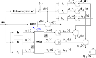
Figure 1: Multiband structure of subband adaptive filter.

In practice, the additive noise $\nu(n)$ can be non-Gaussian consisting of Gaussian and impulsive components  [20, 21, 22, 23, 24, 25, 26, 27, 28, 29, 30, 31, 32, 33, 34, 35, 36, 37, 38, 39, 40, 41, 42, 43, 44, 45, 46, 47, 48, 49, 50, 51, 52, 53, 54, 55, 56, 57, 58, 59, 60, 61, 62, 63, 64, 65, 66, 67, 68, 69, 70, 71, 72, 73, 74, 75, 76, 77, 78, 79, 80, 81, 82, 83, 84, 85, 86, 87, 88, 89, 90, 91, 92], . Hence, for the identification of a sparse vector $\bm{w}^{o}$ in the presence of impulsive noise, we define the following minimization problem:

$$\begin{array}[]{rcl}\begin{aligned} \arg\min_{\bm{w}(k+1)}&\left[||\bm{w}(k+1)-\bm{w}(k)||_{2}^{2}+\rho f(\bm{w}(k+1))\right],\\ \end{aligned}\end{array}$$ (3)

subject to

$$e_{p,i}(k)= \left[1-\mu\phi_{i}(k)\right]e_{i,D}(k),$$ (4a)

$$\phi_{i}(k)= \frac{\varphi^{\prime}(e_{i,D}(k))}{e_{i,D}(k)},$$ (4b)

for subbands $i=1,...,N$, where $e_{p,i}(k)=d_{i,D}(k)-\bm{u}_{i}^{\text{T}}(k)\bm{w}(k+1)$ denotes the a posteriori decimated subband error, $\mu>0$ will be called the step-size in the sequel, and $\phi_{i}(k)$ is called the scaling factor of the $i$-th subband. In (3), $f(\bm{w})$ is a sparsity-aware penalty function and $\rho>0$ is the weight of this penalty term. In (4b), $\varphi^{\prime}(e)\triangleq\frac{\partial\varphi(e)}{\partial e}$, where $\varphi(e)\geq 0$ is an even function of variable $e$, defining the robustness to impulsive noise.

By using the Lagrange multiplier method, we obtain the solution of (3) subject to (4a) as

$$\begin{array}[]{rcl}\begin{aligned} \bm{w}&(k+1)=\bm{w}(k)+\mu\sum_{i=1}^{N}\phi_{i}(k)\frac{e_{i,D}(k)\bm{u}_{i}(k)}{||\bm{u}_{i}(k)||_{2}^{2}}-\\ &\rho\left[f^{\prime}(\bm{w}(k+1))-\sum_{i=1}^{N}\frac{\bm{u}_{i}(k)\bm{u}_{i}^{\text{T}}(k)}{||\bm{u}_{i}(k)||_{2}^{2}}f^{\prime}(\bm{w}(k+1))\right].\end{aligned}\end{array}$$ (5)

Note that the derivation of (5) also uses an approximation in the SAF, that is $\bm{u}_{i}^{\text{T}}(k)\bm{u}_{j}(k)\approx 0$ for $i\neq j$ [1]. Then, by introducing an intermediate estimate $\bm{\psi}(k)$, we propose to implement (5) in two steps:

$$\bm{\psi}(k)= \bm{w}(k)+\mu\sum_{i=1}^{N}\phi_{i}(k)\frac{e_{i,D}(k)\bm{u}_{i}(k)}{||\bm{u}_{i}(k)||_{2}^{2}},$$ (6a)

$$\bm{w}(k+1)= \bm{\psi}(k)-\rho\bm{P}(k),$$ (6b)

where

$$\begin{array}[]{rcl}\begin{aligned} \bm{P}(k)=f^{\prime}(\bm{\psi}(k))-\sum_{i=1}^{N}\frac{\bm{u}_{i}(k)\bm{u}_{i}^{\text{T}}(k)}{||\bm{u}_{i}(k)||_{2}^{2}}f^{\prime}(\bm{\psi}(k)).\end{aligned}\end{array}$$ (7)

This completes the derivation of the update for the SA-RNSAF algorithm. In this algorithm, the steps (6a) and (6b) have their own roles. The former behaves like the RNSAF algorithm to obtain a coarse estimate $\bm{\psi}(k)$ of the sparse vector $\bm{w}^{o}$ in impulsive noise. Subsequently, the step (6b) forces the inactive coefficients in $\bm{\psi}(k)$ to zero, thus obtaining a more accurate sparse estimate $\bm{w}(k+1)$.

It is noteworthy that the parameters $\mu$ and $\rho$ control the SA-RNSAF’s performance. Specifically, the step-size $\mu$ controls the convergence rate and steady-state misadjustment of the algorithm. Moreover, the SA-RNSAF algorithm can be superior to the RNSAF algorithm when dealing with sparse systems, but $\rho$ must be chosen within a theoretically existing range while this range is unpredictable actually (see Remark 1 below). As such, we will derive adaptive recursions for adjusting $\mu$ and $\rho$. However, it is challenging to solve the global optimization problem on $\mu$ and $\rho$, as (6a) and (6b) depend on each other. Interestingly, $\mu$ and $\rho$ mainly affect the steps (6a) and (6b), respectively, thus we can use alternating optimization [93] to solve this global optimization problem. Accordingly, the adaptations of $\mu$ and $\rho$ will be designed independently according to (6a) and (6b), respectively.

III Proposed AOP-SA-RNSAF Algorithm

By using the band-dependent variable step-size (VSS) $\mu_{i}(k)$ and $\rho(k)$ instead of some fixed values, we rearrange (6a) and (6b) as follows:

$$\bm{\psi}(k)= \bm{w}(k)+\sum_{i=1}^{N}\mu_{i}(k)\phi_{i}(k)\frac{e_{i,D}(k)\bm{u}_{i}(k)}{||\bm{u}_{i}(k)||_{2}^{2}},$$ (8a)

$$\bm{w}(k+1)= \bm{\psi}(k)-\rho(k)\bm{P}(k).$$ (8b)

III-A Adaptation of the step-size

By subtracting (8a) from $\bm{w}^{o}$, we obtain

$$\begin{array}[]{rcl}\begin{aligned} \widetilde{\bm{\psi}}(k)=&\widetilde{\bm{w}}(k)-\sum_{i=1}^{N}\mu_{i}(k)\phi_{i}(k)\frac{e_{i,D}(k)\bm{u}_{i}(k)}{||\bm{u}_{i}(k)||_{2}^{2}},\end{aligned}\end{array}$$ (9)

where $\widetilde{\bm{w}}(k)=\bm{w}^{o}-\bm{w}(k)$ and $\widetilde{\bm{\psi}}(k)=\bm{w}^{o}-\bm{\psi}(k)$ define the deviation vectors for the final estimate $\bm{w}(k)$ and the intermediate estimate $\bm{\psi}(k)$ with respect to the true value. By pre-multiplying $\bm{u}_{i}^{\text{T}}(k)$ on both sides of (9) and applying the approximation $\bm{u}_{i}^{\text{T}}(k)\bm{u}_{j}(k)\approx 0$ for $i\neq j$ again, it is established that

$$\begin{array}[]{rcl}\begin{aligned} e_{\varepsilon,i}(k)=\left[1-\mu_{i}(k)\phi_{i}(k)\right]e_{i,D}(k)\end{aligned}\end{array}$$ (10)

for $i=1,2,...,N$, where $e_{\varepsilon,i}(k)=d_{i,D}(k)-\bm{u}_{i}^{\text{T}}(k)\bm{\psi}(k)$ defines the intermediate a posteriori error at the $i$-th subband resulting from the step (6a). By squaring both sides of (10) and taking the expectations over all the terms, the following relation is obtained:

$$\begin{array}[]{rcl}\begin{aligned} \text{E}\{e_{\varepsilon,i}^{2}(k)\}=\left[1-\mu_{i}(k)\phi_{i}(k)\right]^{2}\text{E}\{e_{i,D}^{2}(k)\},\end{aligned}\end{array}$$ (11)

where $\text{E}\{\cdot\}$ denotes the mathematical expectation. In (11), a common assumption is used that the step-size $\mu_{i}(k)$ and the scaling factors $\{\phi_{i}(k)\}_{i=1}^{N}$ are deterministic at iteration $k$ in contrast with the randomness of $e_{i,D}(k)$ [94, 7].

Motivated by [94], we wish to compute the subband step-sizes in such a way that $\text{E}\{e_{\varepsilon,i}^{2}(k)\}=\sigma_{\nu,i}^{2}$, $i=1,2,...,N$, which means that the powers of the intermediate a posteriori subband errors always equal those of the subband noises, where $\sigma_{\nu,i}^{2}\triangleq\text{E}\{\nu_{i,D}^{2}(k)\}$ denotes the power of the $i$-th subband noise excluding impulsive interferences. on this requirement, then from (11) we can obtain the following equation:

$$\begin{array}[]{rcl}\begin{aligned} \mu_{i}(k)\phi_{i}(k)=1-\sqrt{\frac{\sigma_{\nu,i}^{2}}{\sigma_{e_{i,D}}^{2}(k)}},\end{aligned}\end{array}$$ (12)

where $\sigma_{e_{i,D}}^{2}(k)\triangleq\text{E}\{e_{i,D}^{2}(k)\}$ indicates the power of $e_{i,D}(k)$ without impulsive noises. For robust adaptive algorithms with the scaling factors, there is a common property [6, 7] that when impulsive noises happen, the scaling factors $\phi_{i}(k)$ will become very small (close to zero), thereby preventing the adaptation (8a) from the interference caused by impulsive noises. If the impulsive noise is absent, $\phi_{i}(k)$ will approximately equal one to ensure fast convergence. As such, we can change (12) to

$$\begin{array}[]{rcl}\begin{aligned} \mu_{i}(k)=1-\sqrt{\frac{\sigma_{\nu,i}^{2}}{\sigma_{e_{i,D}}^{2}(k)}}.\end{aligned}\end{array}$$ (13)

To implement (13), the statistical quantities $\sigma_{e_{i,D}}^{2}(k)$ and $\sigma_{\nu,i}^{2}$ are replaced with their estimates $\hat{\sigma}_{e_{i,D}}^{2}(k)$ and $\hat{\sigma}_{\nu,i}^{2}(k)$, respectively. Specifically, $\hat{\sigma}_{e_{i,D}}^{2}(k)$ is calculated in an exponential window way as

$$\begin{array}[]{rcl}\begin{aligned} \hat{\sigma}_{e_{i,D}}^{2}(k)=\zeta\hat{\sigma}_{e_{i,D}}^{2}(k-1)+(1-\zeta)\phi_{i}^{2}(k)e_{i,D}^{2}(k),\end{aligned}\end{array}$$ (14)

where $\zeta$ is a weighting factor often chosen as $\zeta=1-1/(\kappa M)$ with $\kappa\geq 1$. Similar to [94], $\hat{\sigma}_{\nu,i}^{2}(k)$ is calculated by the following equations:

$$\hat{\sigma}_{u_{i}}^{2}(k) =\zeta\hat{\sigma}_{u_{i}}^{2}(k-1)+(1-\zeta)u_{i}^{2}(kN),$$ (15a)

$$\hat{\bm{r}}_{ue_{i}}(k) =\zeta\hat{\bm{r}}_{ue_{i}}(k-1)+(1-\zeta)\phi_{i}(k)e_{i,D}(k)\bm{u}_{i}(k),$$ (15b)

$$\hat{\sigma}_{\nu,i}^{2}(k) =\hat{\sigma}_{e_{i,D}}^{2}(k)-\frac{||\hat{\bm{r}}_{ue_{i}}(k)||_{2}^{2}}{\hat{\sigma}_{u_{i}}^{2}(k)+\epsilon_{1}},$$ (15c)

where $\epsilon_{1}$ is a small positive number (e.g., $10^{-5}$). Note that, we introduce the scaling factor $\phi_{i}(k)$ in (14) and (15b) for each subband to suppress impulsive noises.

Accordingly, (13) can be rewritten as

$$\begin{array}[]{rcl}\begin{aligned} \mu_{i}(k)=1-\sqrt{\frac{\hat{\sigma}_{\nu,i}^{2}(k)}{\hat{\sigma}_{e_{i,D}}^{2}(k)+\epsilon_{2}}},\end{aligned}\end{array}$$ (16)

where $\epsilon_{2}$ is also a small positive number. It is stressed that the estimated values of multiple statistical quantities are used in (15c), and thus $\hat{\sigma}_{\nu,i}^{2}(k)$ could be negative at some iterations. To avoid this, we add the step $\hat{\sigma}_{\nu,i}^{2}(k)\leftarrow\hat{\sigma}_{\nu,i}^{2}(k-1)$ after (15c).

III-B Adaptation of the sparsity penalty weight

By subtracting (8b) from $\bm{w}^{o}$, we obtain

$$\begin{array}[]{rcl}\begin{aligned} \widetilde{\bm{w}}(k+1)=\widetilde{\bm{\psi}}(k)+\rho(k)\bm{P}(k).\end{aligned}\end{array}$$ (17)

By pre-multiplying both sides of (17) by their transpose, we obtain

$$\begin{array}[]{rcl}\begin{aligned} ||\widetilde{\bm{w}}&(k+1)||_{2}^{2}=||\widetilde{\bm{\psi}}(k)||_{2}^{2}+\triangle(k),\end{aligned}\end{array}$$ (18)

where

$$\begin{array}[]{rcl}\begin{aligned} \triangle(k)=2\rho(k)\widetilde{\bm{\psi}}^{\text{T}}(k)\bm{P}(k)+\rho^{2}(k)||\bm{P}(k)||_{2}^{2}.\end{aligned}\end{array}$$ (19)

Remark 1: (18) clearly reveals that the proposed SA-RNSAF algorithm will outperform the RNSAF algorithm for identifying sparse systems, if and only if $\triangle(k)<0$ holds. It follows that $\rho(k)$ should satisfy the inequality

$$\begin{array}[]{rcl}\begin{aligned} 0<\rho(k)<2\frac{[\bm{\psi}(k)-\bm{w}^{o}]^{\text{T}}\bm{P}(k)}{||\bm{P}(k)||_{2}^{2}}.\end{aligned}\end{array}$$ (20)

Moreover, since $\triangle(k)$ is the quadratic function of $\rho(k)$, there is an optimal $\rho(k)$ such that $\triangle(k)$ arrives at the negative maximum value. Consequently, the optimal $\rho(k)$ is given as

$$\begin{array}[]{rcl}\begin{aligned} \rho_{\text{opt}}(k)=\frac{[\bm{\psi}(k)-\bm{w}^{o}]^{\text{T}}\bm{P}(k)}{||\bm{P}(k)||_{2}^{2}}.\end{aligned}\end{array}$$ (21)

Although Remark 1 states that the relations (20) and (21) are existing in sparse systems, they are incalculable due to the fact that the sparse vector $\bm{w}^{o}$ is unknown. To solve this problem, we use the previous estimate $\bm{w}(k)$ to approximate $\bm{w}^{o}$, then (21) can be reformulated as

$$\begin{array}[]{rcl}\begin{aligned} \hat{\rho}_{\text{opt}}(k)=\max\left\{\frac{[\bm{\psi}(k)-\bm{w}(k)]^{\text{T}}\bm{P}(k)}{||\bm{P}(k)||_{2}^{2}},0\right\},\end{aligned}\end{array}$$ (22)

where $\hat{\rho}_{\text{opt}}(k)$ is set to zero at $k=0$.

The recursion (8) equipped with $\mu_{i}(k)$ in (16) and $\hat{\rho}_{\text{opt}}(k)$ in (22) constitutes the proposed AOP-SA-RNSAF algorithm.

Remark 2: The proposed AOP-SA-RNSAF update generalizes different algorithms, depending on the choice of $\varphi(e)$ in (4b) and $f(\bm{w})$ in (3). In the literature, several robust criteria against impulsive noises [14, 9, 6, 7, 10] defined by $\varphi(e)$ and sparsity-aware penalties [19, 16, 18, 15, 95] defined by $f(\bm{w})$ have been studied, which can be applied in the AOP-SA-RNSAF. Nevertheless, this paper does not consider the effect of different choices of $\varphi(e)$ and/or $f(\bm{w})$, which is worth studying in future work. Note that, when setting $\varphi(e)=\frac{1}{2}e^{2}$, the proposed algorithm is called the alternating optimization of parameters based SA-NSAF (AOP-SA-NSAF) suited for Gaussian noise environments, which is a sparsity-aware variant of the VSS-NSAF algorithm presented in [94].

Remark 3: By firstly computing the inner product $\bm{u}_{i}^{\text{T}}(k)f^{\prime}(\bm{\psi}(k))$ in $\bm{P}(k)$, and then calculating $\bm{P}(k)$ only requires $2M$ multiplications, $2M-M/N$ additions, and 1 division. Therefore, the complexity of the proposed AOP-SRNSAF algorithm is still low with $\mathcal{O}(M)$ arithmetic operations per input sample.

IV Simulation Results

To evaluate the proposed AOP-SA-RNSAF algorithm, simulations are conducted to identify the acoustic echo paths with $M=512$ taps. The sparsenesses, defined as $\chi(\bm{w}^{o})=\frac{M}{M-\sqrt{M}}\left(1-\frac{||w^{o}||_{1}}{\sqrt{M}||w^{o}||_{2}}\right)$, of two echo paths are $\chi(\bm{w}^{o}_{1})=0.9357$ (sparse) [19] and $\chi(\bm{w}^{o}_{2})=0.3663$ (dispersive or non-sparse) [14], respectively. The length of the adaptive filters is the same as that of $\bm{w}^{o}$. The correlated input signal $u(n)$ is a first-order autoregressive (AR) process with the pole at 0.9, generated by filtering a white Gaussian noise with zero-mean and unit variance. The analysis filters $\{\bm{h}_{i}\}_{i=0}^{N-1}$ for decomposing signals $d(n)$ and $u(n)$ are obtained by cosine-modulated filter banks, where the length of the prototype filter for $N=4$ subbands is 33 to obtain 60 dB stopband attenuation. The high stopband attenuation is to guarantee that adjacent analysis filters have almost no overlap and the cross-correlation of nonadjacent subbands is negligible [2]. The normalized mean square deviation (NMSD), defined as $\text{E}\{||\bm{w}(n)-\bm{w}^{o}||_{2}^{2}/||\bm{w}^{o}||_{2}^{2}\}$, is the performance measure. All the results are the average over 50 independent runs.

For the AOP-SA-RNSAF algorithm, we use the modified Huber (MH) function for $\varphi(e)$ and the log-penalty for $f(\bm{\psi}(k))$. The MH function is formulated as $\varphi(e_{i,D}(k))=e_{i,D}^{2}(k)/2$ if $|e_{i,D}(k)|<\xi_{i}$ and $\varphi(e_{i,D}(k))=0$ if $|e_{i,D}(k)|\geq\xi_{i}$ [10], where $\xi_{i}$ is the threshold. Accordingly, when $|e_{i,D}(k)|\geq\xi_{i}$ (usually impulsive noises occur), then the scaling factor in (4b) is $\phi_{i}(k)=0$, which makes the adaptation step (8a) freeze to suppress impulsive interferences; otherwise, $\phi_{i}(k)=1$, which retains fast convergence. Note that, the threshold $\xi_{i}$ for each subband $i$ is set to $\xi_{i}=2.576\hat{\sigma}_{\varepsilon,i}(k)$, where $\hat{\sigma}_{\varepsilon,i}^{2}(k)$ is the variance of $e_{i,D}(k)$ excluding impulsive samples. $\hat{\sigma}_{\varepsilon,i}^{2}(k)$ is computed by $\hat{\sigma}_{\varepsilon,i}^{2}(k)=\lambda\hat{\sigma}_{\varepsilon,i}^{2}(k-1)+c_{\sigma}(1-\lambda)\text{med}(\bm{a}_{\varepsilon,i})$, where $\lambda\in(0.9,1)$ is the forgetting factor (but $\lambda=0$ at $k=0$), $\text{med}(\cdot)$ denotes the median operator to remove outliers in the data window $\bm{a}_{\varepsilon,i}=[e_{i,D}^{2}(k),e_{i,D}^{2}(k-1),...,e_{i,D}^{2}(k-N_{w}+1)]$ with a length of $N_{w}$, and $c_{\sigma}=1.483(1+5/(N_{w}-1))$ is the correction factor. The log-penalty is given as $f(\bm{\psi}_{k})=\sum_{m=1}^{M}\ln(1+|\psi_{m,k}|/\theta)$ [19] which characterizes the sparsity of systems, where $\psi_{m,k}$ is the $m$-th element of $\bm{\psi}_{k}$, and the shrinkage factor $\theta>0$ cuts apart inactive and active entries in $\bm{\psi}_{k}$. Thus, $f^{\prime}(\bm{\psi}_{m,k})$ in (7) is computed element-wise as $f^{\prime}(\psi_{m,k})=\frac{\text{sgn}(\psi_{m,k})}{\theta+|\psi_{m,k}|},m=1,...,M$. In our simulations, the additive noise $\nu(n)$ is described by the symmetric $\alpha$-stable process, also called the $\alpha$-stable noise, whose characteristic function is formulated as $\phi(t)=\exp(-\gamma\lvert t\lvert^{\alpha})$ [3]. The parameter $\alpha\in(0,2]$ represents the impulsiveness of the noise that for smaller $\alpha$ leads to stronger impulsive noises, and $\gamma>0$ behaves like the variance of the Gaussian density. In particular, it reduces to the Gaussian noise for the case of $\alpha=2$. In the following simulations, we set $\gamma=0.02$.

Example 1: the impulsive noise is absent, i.e., $\alpha=2$. The proposed AOP-SA-NSAF algorithm in Remark 2 is compared with the NSAF, VP-SA-NSAF [18], VSS-NSAF, and VSS-PNSAF algorithms in Fig. 2, where both VSS-NSAF and VSS-PNSAF are obtained from [10] but in the Gaussian noise we reset $\varphi(e)=\frac{1}{2}e^{2}$ instead of using the MH function. For a fair evaluation, we select the log-penalty parameter $\theta=0.005$ for all the sparsity-aware algorithms. As can be seen, the VSS-NSAF algorithm obtains fast convergence and low steady-state misadjustment, which overcomes the trade-off problem in the NSAF algorithm. By considering the sparsity of the underlying system, both VP-SA-NSAF and VSS-PNSAF algorithms further improve the convergence rate. As compared to the VSS-PNSAF algorithm, the proposed AOP-SNSAF algorithm shows slower initial convergence, but it achieves higher reduction in the steady-state misadjustment.

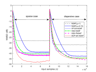
Figure 2: NMSD performance of NSAF-type algorithms in the Gaussian noise. The parameters of algorithms are listed as follows: $\eta=0.99$, $\lambda=0.95$, and $\mu_{\max}=1$ for VP-SA-NSAF; $\tau=3$ for VSS-NSAF; $\tau=5$ and $\zeta=0$ for VSS-PNSAF; $\kappa=6$ for AOP-SA-NSAF.

Example 2: $\alpha=1.6$ displays the presence of impulsive noises. Fig. 3 depicts the NMSD performance of the NSAF, M-NSAF [10], VSS-M-NSAF [10], VSS-M-PNSAF [10], VP-IWF-SSAF with RA [19], and the proposed AOP-SA-RNSAF algorithms. For the M-estimate based algorithms, we choose the common M-estimate parameters $\lambda=0.99$ and $N_{w}=20$. It is seen that the NSAF algorithm shows poor misadjustment in the $\alpha$-stable noise, and other algorithms exhibit robust convergence. Among these robust algorithms, the proposed AOP-SA-RNSAF algorithm is the best choice for identifying sparse systems, due to the fact that it has lower steady-state misadjustment than the VSS-M-PNSAF and VP-S-IWF-SSAF with RA algorithms, even if it has a slightly slower initial convergence than the VSS-M-PNSAF algorithm.

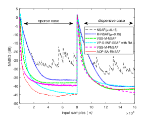
Figure 3: NMSD performance of NSAF-type algorithms in the $\alpha$-stable noise. The parameters of algorithms are listed as follows: $\mu_{\min}=10^{-5}$, $\tau=2$, and $\chi=1$ for VP-S-IWF-SSAF; $\tau=3$ for VSS-M-NSAF; $\tau=5$ and $\zeta=0$ for VSS-M-PNSAF; $\kappa=6$ for AOP-SA-RNSAF.

It can be seen in Figs. 2 and 3 that, after $\bm{w}^{o}$ becomes dispersive at the middle of input samples, the proportionate-type (i.e., VSS-PNSAF, VSS-PNSAF) and sparsity-aware type (i.e., VP-SA-NSAF, AOP-SA-NSAF, AOP-SA-RNSAF) algorithms still show almost the same performance as the competing algorithms (i.e., VSS-NSAF and VSS-M-NSAF) in both Gaussian and $\alpha$-stable noise scenarios. In addition, as $\alpha$ decreases from 2 to 1.6, the steady-state misadjustment of the proposed AOP-SA-RNSAF algorithm increases, but this algorithm is still convergent.

V Conclusion

In this paper, a unified SA-RNSAF framework for algorithms was developed for identifying sparse systems in impulsive noise environments. By replacing directly the specified robustness criterion and sparsity-aware penalty, it can yield different SA-RNSAF algorithms. We then developed adaptive techniques for the step-size and the sparsity penalty weight in the SA-RNSAF algorithm, thus arriving at the AOP-SA-RNSAF algorithm with a further performance improvement in terms of the convergence rate and steady-state misadjustment. Simulations for the sparse system identification have demonstrated the effectiveness of the proposed algorithms.

References

- [1] K.-A. Lee and W.-S. Gan, “Improving convergence of the NLMS algorithm using constrained subband updates,” IEEE Signal Processing Letters, vol. 11, no. 9, pp. 736–739, 2004.
- [2] K.-A. Lee, W.-S. Gan, and S. M. Kuo, Subband adaptive filtering: theory and implementation. John Wiley & Sons, 2009.
- [3] C. L. Nikias and M. Shao, Signal processing with Alpha-stable distributions and applications. Wiley-Interscience, 1995.
- [4] M. Zimmermann and K. Dostert, “Analysis and modeling of impulsive noise in broad-band powerline communications,” IEEE Transactions on Electromagnetic Compatibility, vol. 44, no. 1, pp. 249–258, 2002.
- [5] J.-H. Kim, J. Kim, J. H. Jeon, and S. W. Nam, “Delayless individual-weighting-factors sign subband adaptive filter with band-dependent variable step-sizes,” IEEE/ACM Transactions on Audio, Speech, and Language Processing, vol. 25, no. 7, pp. 1526–1534, 2017.
- [6] F. Huang, J. Zhang, and S. Zhang, “Combined-step-size normalized subband adaptive filter with a variable-parametric step-size scaler against impulsive interferences,” IEEE Transactions on Circuits and Systems II: Express Briefs, vol. 65, no. 11, pp. 1803–1807, 2017.
- [7] J. Hur, I. Song, and P. Park, “A variable step-size normalized subband adaptive filter with a step-size scaler against impulsive measurement noise,” IEEE Transactions on Circuits and Systems II: Express Briefs, vol. 64, no. 7, pp. 842–846, 2016.
- [8] Z. Zheng, Z. Liu, and X. Lu, “Robust normalized subband adaptive filter algorithm against impulsive noises and noisy inputs,” Journal of the Franklin Institute, vol. 357, no. 5, pp. 3113–3134, 2020.
- [9] Y. Yu, H. Zhao, B. Chen, and Z. He, “Two improved normalized subband adaptive filter algorithms with good robustness against impulsive interferences,” Circuits, Systems, and Signal Processing, vol. 35, no. 12, pp. 4607–4619, 2016.
- [10] Y. Yu, H. He, B. Chen, J. Li, Y. Zhang, and L. Lu, “M-estimate based normalized subband adaptive filter algorithm: Performance analysis and improvements,” IEEE/ACM Transactions on Audio, Speech, and Language Processing, vol. 28, pp. 225–239, 2020.
- [11] J. Radecki, Z. Zilic, and K. Radecka, “Echo cancellation in IP networks,” in The 45th Midwest Symposium on Circuits and Systems (MWSCAS), vol. 2, 2002, pp. II–II.
- [12] W. F. Schreiber, “Advanced television systems for terrestrial broadcasting: Some problems and some proposed solutions,” Proceedings of the IEEE, vol. 83, no. 6, pp. 958–981, 1995.
- [13] M. S. E. Abadi and S. Kadkhodazadeh, “A family of proportionate normalized subband adaptive filter algorithms,” Journal of the Franklin Institute, vol. 348, no. 2, pp. 212–238, 2011.
- [14] Z. Zheng, Z. Liu, H. Zhao, Y. Yu, and L. Lu, “Robust set-membership normalized subband adaptive filtering algorithms and their application to acoustic echo cancellation,” IEEE Transactions on Circuits and Systems I: Regular Papers, vol. 64, no. 8, pp. 2098–2111, 2017.
- [15] Y. Yu, H. Zhao, R. C. de Lamare, and L. Lu, “Sparsity-aware subband adaptive algorithms with adjustable penalties,” Digital Signal Processing, vol. 84, pp. 93–106, 2019.
- [16] E. Heydari, M. S. E. Abadi, and S. M. Khademiyan, “Improved multiband structured subband adaptive filter algorithm with l0-norm regularization for sparse system identification,” Digital Signal Processing, p. 103348, 2021.
- [17] N. Puhan and G. Panda, “Zero attracting proportionate normalized subband adaptive filtering technique for feedback cancellation in hearing aids,” Applied Acoustics, vol. 149, pp. 39–45, 2019.
- [18] L. Ji and J. Ni, “Sparsity-aware normalized subband adaptive filters with jointly optimized parameters,” Journal of the Franklin Institute, vol. 357, no. 17, pp. 13 144–13 157, 2020.
- [19] Y. Yu, T. Yang, H. Chen, R. C. de Lamare, and Y. Li, “Sparsity-aware ssaf algorithm with individual weighting factors: Performance analysis and improvements in acoustic echo cancellation,” Signal Processing, vol. 178, p. 107806, 2021.
- [20] R. C. de Lamare and R. Sampaio-Neto, “Adaptive reduced-rank processing based on joint and iterative interpolation, decimation, and filtering,” IEEE Transactions on Signal Processing, vol. 57, no. 7, pp. 2503–2514, 2009.
- [21] R. C. de Lamare and R. Sampaio-Neto, “Minimum mean-squared error iterative successive parallel arbitrated decision feedback detectors for ds-cdma systems,” IEEE Transactions on Communications, vol. 56, no. 5, pp. 778–789, 2008.
- [22] R. de Lamare and R. Sampaio-Neto, “Adaptive reduced-rank mmse filtering with interpolated fir filters and adaptive interpolators,” IEEE Signal Processing Letters, vol. 12, no. 3, pp. 177–180, 2005.
- [23] R. C. de Lamare, “Adaptive and iterative multi-branch mmse decision feedback detection algorithms for multi-antenna systems,” IEEE Transactions on Wireless Communications, vol. 12, no. 10, pp. 5294–5308, 2013.
- [24] R. C. de Lamare and R. Sampaio-Neto, “Reduced-rank adaptive filtering based on joint iterative optimization of adaptive filters,” IEEE Signal Processing Letters, vol. 14, no. 12, pp. 980–983, 2007.
- [25] R. C. de Lamare and R. Sampaio-Neto, “Reduced-rank space-time adaptive interference suppression with joint iterative least squares algorithms for spread-spectrum systems,” IEEE Transactions on Vehicular Technology, vol. 59, no. 3, pp. 1217–1228, 2010.
- [26] R. C. de Lamare and R. Sampaio-Neto, “Adaptive reduced-rank equalization algorithms based on alternating optimization design techniques for mimo systems,” IEEE Transactions on Vehicular Technology, vol. 60, no. 6, pp. 2482–2494, 2011.
- [27] R. Fa, R. C. de Lamare, and L. Wang, “Reduced-rank stap schemes for airborne radar based on switched joint interpolation, decimation and filtering algorithm,” IEEE Transactions on Signal Processing, vol. 58, no. 8, pp. 4182–4194, 2010.
- [28] R. C. de Lamare, M. Haardt, and R. Sampaio-Neto, “Blind adaptive constrained reduced-rank parameter estimation based on constant modulus design for cdma interference suppression,” IEEE Transactions on Signal Processing, vol. 56, no. 6, pp. 2470–2482, 2008.
- [29] P. Clarke and R. C. de Lamare, “Transmit diversity and relay selection algorithms for multirelay cooperative mimo systems,” IEEE Transactions on Vehicular Technology, vol. 61, no. 3, pp. 1084–1098, 2012.
- [30] P. Li and R. C. De Lamare, “Adaptive decision-feedback detection with constellation constraints for mimo systems,” IEEE Transactions on Vehicular Technology, vol. 61, no. 2, pp. 853–859, 2012.
- [31] Z. Yang, R. C. de Lamare, and X. Li, “¡formula formulatype=”inline”¿¡tex notation=”tex”¿¡/tex¿ ¡/formula¿-regularized stap algorithms with a generalized sidelobe canceler architecture for airborne radar,” IEEE Transactions on Signal Processing, vol. 60, no. 2, pp. 674–686, 2012.
- [32] R. de Lamare and R. Sampaio-Neto, “Adaptive mber decision feedback multiuser receivers in frequency selective fading channels,” IEEE Communications Letters, vol. 7, no. 2, pp. 73–75, 2003.
- [33] R. de Lamare, L. Wang, and R. Fa, “Adaptive reduced-rank lcmv beamforming algorithms based on joint iterative optimization of filters: Design and analysis,” Signal Processing, vol. 90, no. 2, pp. 640–652, 2010. [Online]. Available: https://www.sciencedirect.com/science/article/pii/S0165168409003466
- [34] H. Ruan and R. C. de Lamare, “Robust adaptive beamforming using a low-complexity shrinkage-based mismatch estimation algorithm,” IEEE Signal Processing Letters, vol. 21, no. 1, pp. 60–64, 2014.
- [35] R. C. de Lamare and P. S. R. Diniz, “Set-membership adaptive algorithms based on time-varying error bounds for cdma interference suppression,” IEEE Transactions on Vehicular Technology, vol. 58, no. 2, pp. 644–654, 2009.
- [36] R. de Lamare and R. Sampaio-Neto, “Blind adaptive code-constrained constant modulus algorithms for cdma interference suppression in multipath channels,” IEEE Communications Letters, vol. 9, no. 4, pp. 334–336, 2005.
- [37] S. Xu, R. C. de Lamare, and H. V. Poor, “Distributed compressed estimation based on compressive sensing,” IEEE Signal Processing Letters, vol. 22, no. 9, pp. 1311–1315, 2015.
- [38] R. C. De Lamare, R. Sampaio-Neto, and A. Hjorungnes, “Joint iterative interference cancellation and parameter estimation for cdma systems,” IEEE Communications Letters, vol. 11, no. 12, pp. 916–918, 2007.
- [39] R. Fa and R. C. De Lamare, “Reduced-rank stap algorithms using joint iterative optimization of filters,” IEEE Transactions on Aerospace and Electronic Systems, vol. 47, no. 3, pp. 1668–1684, 2011.
- [40] R. C. de Lamare and R. Sampaio-Neto, “Adaptive interference suppression for ds-cdma systems based on interpolated fir filters with adaptive interpolators in multipath channels,” IEEE Transactions on Vehicular Technology, vol. 56, no. 5, pp. 2457–2474, 2007.
- [41] R. C. De Lamare and R. Sampaio-Neto, “Blind adaptive mimo receivers for space-time block-coded ds-cdma systems in multipath channels using the constant modulus criterion,” IEEE Transactions on Communications, vol. 58, no. 1, pp. 21–27, 2010.
- [42] R. de Lamare and R. Sampaio-Neto, “Low-complexity variable step-size mechanisms for stochastic gradient algorithms in minimum variance cdma receivers,” IEEE Transactions on Signal Processing, vol. 54, no. 6, pp. 2302–2317, 2006.
- [43] A. G. D. Uchoa, C. T. Healy, and R. C. de Lamare, “Iterative detection and decoding algorithms for mimo systems in block-fading channels using ldpc codes,” IEEE Transactions on Vehicular Technology, vol. 65, no. 4, pp. 2735–2741, 2016.
- [44] R. Fa, “Multi-branch successive interference cancellation for mimo spatial multiplexing systems: design, analysis and adaptive implementation,” IET Communications, vol. 5, pp. 484–494(10), March 2011. [Online]. Available: https://digital-library.theiet.org/content/journals/10.1049/iet-com.2009.0843
- [45] N. Song, R. C. de Lamare, M. Haardt, and M. Wolf, “Adaptive widely linear reduced-rank interference suppression based on the multistage wiener filter,” IEEE Transactions on Signal Processing, vol. 60, no. 8, pp. 4003–4016, 2012.
- [46] L. T. N. Landau and R. C. de Lamare, “Branch-and-bound precoding for multiuser mimo systems with 1-bit quantization,” IEEE Wireless Communications Letters, vol. 6, no. 6, pp. 770–773, 2017.
- [47] H. Ruan and R. C. de Lamare, “Robust adaptive beamforming based on low-rank and cross-correlation techniques,” IEEE Transactions on Signal Processing, vol. 64, no. 15, pp. 3919–3932, 2016.
- [48] S. D. Somasundaram, N. H. Parsons, P. Li, and R. C. de Lamare, “Reduced-dimension robust capon beamforming using krylov-subspace techniques,” IEEE Transactions on Aerospace and Electronic Systems, vol. 51, no. 1, pp. 270–289, 2015.
- [49] T. Wang, R. C. de Lamare, and P. D. Mitchell, “Low-complexity set-membership channel estimation for cooperative wireless sensor networks,” IEEE Transactions on Vehicular Technology, vol. 60, no. 6, pp. 2594–2607, 2011.
- [50] T. Peng, R. C. de Lamare, and A. Schmeink, “Adaptive distributed space-time coding based on adjustable code matrices for cooperative mimo relaying systems,” IEEE Transactions on Communications, vol. 61, no. 7, pp. 2692–2703, 2013.
- [51] N. Song, W. U. Alokozai, R. C. de Lamare, and M. Haardt, “Adaptive widely linear reduced-rank beamforming based on joint iterative optimization,” IEEE Signal Processing Letters, vol. 21, no. 3, pp. 265–269, 2014.
- [52] R. Meng, R. C. de Lamare, and V. H. Nascimento, “Sparsity-aware affine projection adaptive algorithms for system identification,” in Sensor Signal Processing for Defence (SSPD 2011), 2011, pp. 1–5.
- [53] J. Liu and R. C. de Lamare, “Low-latency reweighted belief propagation decoding for ldpc codes,” IEEE Communications Letters, vol. 16, no. 10, pp. 1660–1663, 2012.
- [54] R. C. de Lamare and R. Sampaio-Neto, “Sparsity-aware adaptive algorithms based on alternating optimization and shrinkage,” IEEE Signal Processing Letters, vol. 21, no. 2, pp. 225–229, 2014.
- [55] L. Wang, “Constrained adaptive filtering algorithms based on conjugate gradient techniques for beamforming,” IET Signal Processing, vol. 4, pp. 686–697(11), December 2010. [Online]. Available: https://digital-library.theiet.org/content/journals/10.1049/iet-spr.2009.0243
- [56] Y. Cai, R. C. d. Lamare, and R. Fa, “Switched interleaving techniques with limited feedback for interference mitigation in ds-cdma systems,” IEEE Transactions on Communications, vol. 59, no. 7, pp. 1946–1956, 2011.
- [57] Y. Cai and R. C. de Lamare, “Space-time adaptive mmse multiuser decision feedback detectors with multiple-feedback interference cancellation for cdma systems,” IEEE Transactions on Vehicular Technology, vol. 58, no. 8, pp. 4129–4140, 2009.
- [58] Z. Shao, R. C. de Lamare, and L. T. N. Landau, “Iterative detection and decoding for large-scale multiple-antenna systems with 1-bit adcs,” IEEE Wireless Communications Letters, vol. 7, no. 3, pp. 476–479, 2018.
- [59] R. de Lamare, “Joint iterative power allocation and linear interference suppression algorithms for cooperative ds-cdma networks,” IET Communications, vol. 6, pp. 1930–1942(12), September 2012. [Online]. Available: https://digital-library.theiet.org/content/journals/10.1049/iet-com.2011.0508
- [60] P. Li and R. C. de Lamare, “Distributed iterative detection with reduced message passing for networked mimo cellular systems,” IEEE Transactions on Vehicular Technology, vol. 63, no. 6, pp. 2947–2954, 2014.
- [61] Y. Cai, R. C. de Lamare, B. Champagne, B. Qin, and M. Zhao, “Adaptive reduced-rank receive processing based on minimum symbol-error-rate criterion for large-scale multiple-antenna systems,” IEEE Transactions on Communications, vol. 63, no. 11, pp. 4185–4201, 2015.
- [62] C. T. Healy and R. C. de Lamare, “Design of ldpc codes based on multipath emd strategies for progressive edge growth,” IEEE Transactions on Communications, vol. 64, no. 8, pp. 3208–3219, 2016.
- [63] L. Wang, R. C. de Lamare, and M. Haardt, “Direction finding algorithms based on joint iterative subspace optimization,” IEEE Transactions on Aerospace and Electronic Systems, vol. 50, no. 4, pp. 2541–2553, 2014.
- [64] J. Gu, R. C. de Lamare, and M. Huemer, “Buffer-aided physical-layer network coding with optimal linear code designs for cooperative networks,” IEEE Transactions on Communications, vol. 66, no. 6, pp. 2560–2575, 2018.
- [65] S. Xu, R. C. de Lamare, and H. V. Poor, “Adaptive link selection algorithms for distributed estimation,” EURASIP J. Adv. Signal Process., vol. 86, 2015.
- [66] L. Wang, R. C. de Lamare, and Y. Long Cai, “Low-complexity adaptive step size constrained constant modulus sg algorithms for adaptive beamforming,” Signal Processing, vol. 89, no. 12, pp. 2503–2513, 2009. [Online]. Available: https://www.sciencedirect.com/science/article/pii/S0165168409001716
- [67] L. Qiu, Y. Cai, R. C. de Lamare, and M. Zhao, “Reduced-rank doa estimation algorithms based on alternating low-rank decomposition,” IEEE Signal Processing Letters, vol. 23, no. 5, pp. 565–569, 2016.
- [68] M. Yukawa, R. C. de Lamare, and R. Sampaio-Neto, “Efficient acoustic echo cancellation with reduced-rank adaptive filtering based on selective decimation and adaptive interpolation,” IEEE Transactions on Audio, Speech, and Language Processing, vol. 16, no. 4, pp. 696–710, 2008.
- [69] S. Xu, “Distributed estimation over sensor networks based on distributed conjugate gradient strategies,” IET Signal Processing, vol. 10, pp. 291–301(10), May 2016. [Online]. Available: https://digital-library.theiet.org/content/journals/10.1049/iet-spr.2015.0384
- [70] L. Landau, “Robust adaptive beamforming algorithms using the constrained constant modulus criterion,” IET Signal Processing, vol. 8, pp. 447–457(10), July 2014. [Online]. Available: https://digital-library.theiet.org/content/journals/10.1049/iet-spr.2013.0166
- [71] L. Wang and R. C. de Lamare, “Adaptive constrained constant modulus algorithm based on auxiliary vector filtering for beamforming,” IEEE Transactions on Signal Processing, vol. 58, no. 10, pp. 5408–5413, 2010.
- [72] Y. Cai and R. C. de Lamare, “Adaptive linear minimum ber reduced-rank interference suppression algorithms based on joint and iterative optimization of filters,” IEEE Communications Letters, vol. 17, no. 4, pp. 633–636, 2013.
- [73] T. G. Miller, S. Xu, R. C. de Lamare, and H. V. Poor, “Distributed spectrum estimation based on alternating mixed discrete-continuous adaptation,” IEEE Signal Processing Letters, vol. 23, no. 4, pp. 551–555, 2016.
- [74] P. Clarke and R. C. de Lamare, “Low-complexity reduced-rank linear interference suppression based on set-membership joint iterative optimization for ds-cdma systems,” IEEE Transactions on Vehicular Technology, vol. 60, no. 9, pp. 4324–4337, 2011.
- [75] S. Li, R. C. de Lamare, and R. Fa, “Reduced-rank linear interference suppression for ds-uwb systems based on switched approximations of adaptive basis functions,” IEEE Transactions on Vehicular Technology, vol. 60, no. 2, pp. 485–497, 2011.
- [76] F. G. Almeida Neto, R. C. De Lamare, V. H. Nascimento, and Y. V. Zakharov, “Adaptive reweighting homotopy algorithms applied to beamforming,” IEEE Transactions on Aerospace and Electronic Systems, vol. 51, no. 3, pp. 1902–1915, 2015.
- [77] W. S. Leite and R. C. De Lamare, “List-based omp and an enhanced model for doa estimation with non-uniform arrays,” IEEE Transactions on Aerospace and Electronic Systems, pp. 1–1, 2021.
- [78] T. Wang, R. C. de Lamare, and A. Schmeink, “Joint linear receiver design and power allocation using alternating optimization algorithms for wireless sensor networks,” IEEE Transactions on Vehicular Technology, vol. 61, no. 9, pp. 4129–4141, 2012.
- [79] R. C. de Lamare and P. S. R. Diniz, “Blind adaptive interference suppression based on set-membership constrained constant-modulus algorithms with dynamic bounds,” IEEE Transactions on Signal Processing, vol. 61, no. 5, pp. 1288–1301, 2013.
- [80] Y. Cai and R. C. de Lamare, “Low-complexity variable step-size mechanism for code-constrained constant modulus stochastic gradient algorithms applied to cdma interference suppression,” IEEE Transactions on Signal Processing, vol. 57, no. 1, pp. 313–323, 2009.
- [81] Y. Cai, R. C. de Lamare, M. Zhao, and J. Zhong, “Low-complexity variable forgetting factor mechanism for blind adaptive constrained constant modulus algorithms,” IEEE Transactions on Signal Processing, vol. 60, no. 8, pp. 3988–4002, 2012.
- [82] M. F. Kaloorazi and R. C. de Lamare, “Subspace-orbit randomized decomposition for low-rank matrix approximations,” IEEE Transactions on Signal Processing, vol. 66, no. 16, pp. 4409–4424, 2018.
- [83] R. B. Di Renna and R. C. de Lamare, “Adaptive activity-aware iterative detection for massive machine-type communications,” IEEE Wireless Communications Letters, vol. 8, no. 6, pp. 1631–1634, 2019.
- [84] H. Ruan and R. C. de Lamare, “Distributed robust beamforming based on low-rank and cross-correlation techniques: Design and analysis,” IEEE Transactions on Signal Processing, vol. 67, no. 24, pp. 6411–6423, 2019.
- [85] S. F. B. Pinto and R. C. de Lamare, “Multistep knowledge-aided iterative esprit: Design and analysis,” IEEE Transactions on Aerospace and Electronic Systems, vol. 54, no. 5, pp. 2189–2201, 2018.
- [86] Y. V. Zakharov, V. H. Nascimento, R. C. De Lamare, and F. G. De Almeida Neto, “Low-complexity dcd-based sparse recovery algorithms,” IEEE Access, vol. 5, pp. 12 737–12 750, 2017.
- [87]
- [88] S. Li and R. C. de Lamare, “Blind reduced-rank adaptive receivers for ds-uwb systems based on joint iterative optimization and the constrained constant modulus criterion,” IEEE Transactions on Vehicular Technology, vol. 60, no. 6, pp. 2505–2518, 2011.
- [89] X. Wu, Y. Cai, M. Zhao, R. C. de Lamare, and B. Champagne, “Adaptive widely linear constrained constant modulus reduced-rank beamforming,” IEEE Transactions on Aerospace and Electronic Systems, vol. 53, no. 1, pp. 477–492, 2017.
- [90] Y. Yu, H. He, T. Yang, X. Wang, and R. C. de Lamare, “Diffusion normalized least mean m-estimate algorithms: Design and performance analysis,” IEEE Transactions on Signal Processing, vol. 68, pp. 2199–2214, 2020.
- [91] R. B. Di Renna and R. C. de Lamare, “Iterative list detection and decoding for massive machine-type communications,” IEEE Transactions on Communications, vol. 68, no. 10, pp. 6276–6288, 2020.
- [92] L. Wang, “Set-membership constrained conjugate gradient adaptive algorithm for beamforming,” IET Signal Processing, vol. 6, pp. 789–797(8), October 2012. [Online]. Available: https://digital-library.theiet.org/content/journals/10.1049/iet-spr.2011.0324
- [93] M. Hong, Z.-Q. Luo, and M. Razaviyayn, “Convergence analysis of alternating direction method of multipliers for a family of nonconvex problems,” SIAM Journal on Optimization, vol. 26, no. 1, pp. 337–364, 2016.
- [94] J. Ni and F. Li, “A variable step-size matrix normalized subband adaptive filter,” IEEE Transactions on Audio, Speech, and Language Processing, vol. 18, no. 6, pp. 1290–1299, 2010.
- [95] R. C. de Lamare and R. Sampaio-Neto, “Sparsity-aware adaptive algorithms based on alternating optimization and shrinkage,” IEEE Signal Processing Letters, vol. 21, no. 2, pp. 225–229, 2014.