Unsupervised Abnormal Traffic Detection through Topological Flow Analysis

Abstract

Cyberthreats are a permanent concern in our modern technological world. In the recent years, sophisticated traffic analysis techniques and anomaly detection (AD) algorithms have been employed to face the more and more subversive adversarial attacks. A malicious intrusion, defined as an invasive action intending to illegally exploit private resources, manifests through unusual data traffic and/or abnormal connectivity pattern. Despite the plethora of statistical or signature-based detectors currently provided in the literature, the topological connectivity component of a malicious flow is less exploited. Furthermore, a great proportion of the existing statistical intrusion detectors are based on supervised learning, that relies on labeled data. By viewing network flows as weighted directed interactions between a pair of nodes, in this paper we present a simple method that facilitate the use of connectivity graph features in unsupervised anomaly detection algorithms. We test our methodology on real network traffic datasets and observe several improvements over standard AD.

I Introduction

Nowadays computer security has become a necessity brought by the fast evolution of information technologies. The expansion of the network architectures, such as cloud computing, revealed increasingly higher number of threats than before. According to 2021 Cyberthreat Defense Report [1], the percentage of organizations compromised by successful attacks rose by 5.5 %, which seems to be the largest in the last 7 years. These attacks include malware, ransomware, Denial-of-Service (DoS) and Advanced Persistent Threats (APT). Despite the fact that security research investments are on a positive trend, alleviation of these threats is not optimistic [1]. However, the constant progress and performance of the recent Intrusion Detection Systems (IDS) bring a positive light on the subject.

One side of the modern IDSs approaches the intrusion detection as an anomaly detection problem. Detecting outliers in finite samples of data is an old statistical topic, alongside with the design of robust estimators that are resistant to corrupted data points [2]. From this viewpoint, detecting a network intrusion reduces to learning a statistical estimator that is capable to distinguish between normal and abnormal traffic. However, there are two obvious issues to address. Related to first, one could find a plethora of results in the literature that confirm the efficiency of this statistical approach for usual attacks such as DoS, Probe, User to Root, Remote to User etc. However, in large networks, there is often the case when the attacker uses a stolen set of credentials to obtain data (or access) from (to) multiple nodes of the networks. In this case, while the traffic parameters may seem close to normal, the change in the graph connectivity pattern could reveal an abnormal behavior. In his malicious pursuit, the attacker will probably walk from node to node, through lateral movement, on paths that a normal user would never follow. Therefore, the underlying graph representation of the network traffic, where the nodes are the computers and the edges are the traffic sessions, becomes necessary. Secondly, the real network traffic is by nature not labeled. Although the most challenging, unsupervised AD methods seems the most intuitive approach of an intrusion detection task.

In this paper we bring a preliminary evidence showing that the graph connectivity may be an important asset in some cases for unsupervised intrusion detection. We design a simple processing strategy of given flow data that enrich the feature vectors with additional graph embeddings. Our graph embedding method is based on computing egonets of each network node and extract their key features. After training on the extended features, the accuracy of several unsupervised AD algorithms shows slight improvements.

I-A Related work

Several wide-range anomaly detection techniques that are often used in network IDSs are listed as follows: Statistical Profiling with Histograms [3, 4], Parametric and Non-parametric Statistical Modeling [5, 6], (Deep or Shallow) Artificial Neural Networks and Autoencoders [7, 8, 9, 10], (One-Class) Support Vector Machines [11, 12], Reconstruction methods [13, 14, 15], Clustering methods [16, 17]. However, generally most of these learning systems detect abnormal data flows or packets based on their features and characteristics. Besides the track imprinted in these features, many attacks manifest their tracks into anomalous underlying connection graph, and therefore graph anomaly detection techniques become an important tool for more insight [18].

Graph embedding is used in [19], where the flow data is viewed as an entropy time series, whose features are mapped as nodes in an undirected graph. Here, after computing weights on edges based on covariance between features, the authors devise an algorithm that assign an anomaly score on each flow. Spectral decomposition methods are applied in [20] to intrusion detection problem. Their method keeps only statistical and spectral features of a given connectivity graph to detect traffic anomalies. In [21] are used attack graphs to analyze the state evolution of multi-layered attacks in a vulnerable system. We mention that the vertices in these graphs are the attack states and actions, since they serve to modeling of the causality of vulnerability exploitation.

In [22] the authors devise an IDS that, based on a double graph embedding, expand an original set of features into a new one containing graph embedding information. Their overall approach is vaguely similar to ours, however the embedding procedure and classification algorithms are not related. In the final, they used supervised learning algorithms to classify enhanced features of datasets CIDDS-001 and CIC-IDS2017.

Paper structure. In the following Section we describe our graph embedding and feature expansion procedures. We evaluate the empirical performance of these embedding procedures, in Section III, by comparison with the application of traditional anomaly detectors onto several well-known datasets. Lastly, we discuss and interpret our result in Section IV.

II Methodology

As presented in the introduction, the main steps of our method reduce to: $(i)$ embedding of the network flows into a directed graph; $(ii)$ extraction of several statistical node features from the graph and expand the original feature set. We use notation $X\in\mathbf{R}^{m\times N}$ for flow data, where $m$ is the number of features of a given flow and $N$ the number of flows.

First, given a set of fixed IPs within a network, mapping them into integers set $[n]:=\{1,2,\cdots,n\}$, where $n$ is the number of machines in the network, is straightforward. Now we further consider the graph $\mathcal{G}=\{V,E,W\}$, where the set of vertices $V=\{1,2,\cdots,n\}$, $E$ is the set of edges between nodes, corresponding to connections between pairs of IPs, and $W$ is a weight matrix. For instance, given a flow representation between two IPs let $(i,j)\equiv(\text{source}\_IP,\text{destination}\_IP)$, then $(i,j)\in E$ if there exists a flow between IPs mappings $(i,j)$ and the value $w_{ij}$ on $i$th column and $j$th line in matrix $W$ defines some summable feature, for example the number of packets transmitted between source and destination.

Figure 1: Subgraph enclosed by dashed line represents the egonet of node 1.

An egonet of node $i$ is defined as the subgraph formed by all neighbors linked to node $i$ [18], as described by Figure 1. Notice that egonets associated to different nodes may have different dimensions, depending on the degree of each node.

Mainly, our scheme consists of the following three steps:

I. Flow-to-graph. The first step performs the conversion of data from flow format into graph format, by retaining source, destination addresses $(i,j)$ and a particular attribute which represents the weight $w_{ij}$. This particular attribute may be any real-valued summable feature in the original data $X$. Since multiple flows may occur multiple times between the same pair of nodes, we get multiple weights $w_{ij}^{t}$, where $t$ is time counter. We sum over $t$ these weights in order to obtain a final weight: $w_{ij}=\sum_{t}w_{ij}^{t}$.

Based on the obtained graph features and weights, we form the directed graph associated with our data.

II. Graph-to-features. Now on this resulted graph we perform the following operations:

1. Extract all the egonets and stack them into $\mathcal{E}$, where each $\mathcal{E}_{i}\in\mathcal{E}$ is the egonet associated to node $i\in V$.

2. Extract a random-walk of size $\ell$ for each node. Denote $\mathcal{E}_{i}\in\mathcal{E}$ as the random-walk associated to node $i$ in $V$. Starting at node $i$, for at most $\ell$ iterations, a neighbor of the current node is randomly chosen (w.r.t. a uniform probability distribution) and its associated edge is added to the subset $\mathcal{E}_{i}$. The new chosen node becomes the current node and a new iteration is performed. If either the node $i$ or the walk length $\ell$ are reached, the process terminates and outputs the walk.

3. For any $i\in[n]$, extract $p$ features of the egonet/random walk instance $\mathcal{E}_{i}$. Denote $z_{i}\in\mathbf{R}^{p}$ the vector of these features.

4. Output matrix $Z\in\mathbf{R}^{p\times n}$, as the array containing all egonet features.

First we perfom only once a single step of the two alternatives $1)$ or $1^{\prime})$. Notice that the random-walk $\mathcal{E}_{i}$ computed in scenario $1^{\prime})$ is not limited to the egonet neighborhood of node $i$. The statistical features computed in step $2)$, after step $1)$, include: dimension of egonet, the number of out-links, the number of in-links. In alternative scenario $1^{\prime})$ they include the weight on the first leg of the walk or the weight transferred all the way from the first node to the last one of the walk. The full description of all features can be find in [23].

III. Feature expansion. Lastly, we expand the original data by adding the columns of $Z$ as prolongation of columns in $X$. Thus, for a given flow $x_{t}\in X$ from source $i$ to destination $j$, we form:

$$\hat{x}_{t}=\begin{bmatrix}x_{t}\\ z_{i}\\ z_{j}\end{bmatrix}\in\mathbf{R}^{m+2p}.$$

The matrix $\hat{X}$ containing columns $\hat{x}_{t}$ for $t\in[N]$ is the output of our scheme.

First, notice that the graph embedding at step II maps the flows from $X$ with size $m\times N$ into a final matrix $Z$ with size $p\times n$. By comparison, a column sample of $X$ corresponds to an edge/flow in the graph, while in $Z$ a column associates with a node. In the next section, we show the performance of AD tools in detecting anomalous nodes.

Second, the step III is equivalent with inserting local topological information into flow features. Therefore the attacks that forces anomalous connections between machines are likely to be reflected into graph features $\{z_{i},z_{j}\}$ and detected by an usual anomaly detection.

We further test the performance of several anomaly detections such as: One Class-SVM, Isolation Forests and Local Outlier Factor, onto the data output of the above processing procedure.

TABLE I: Maximum balanced accuracy and running times when tuning parameters on 1% of the available data.

Dataset	Method	($m$,$N$,outliers)	OC-SVM		LOF		IForest		Ensemble
CIC-IDS2017	standard	(87, 4588, 5)	0.8751	0.81s	0.9751	0.01s	0.8751	0.07s	0.9152
	graph	(48, 382, 1)	0.9252	0.02s	0.9685	0.01s	0.4738	0.04s	0.8972
	mixed	(183, 4588, 5)	0.8167	5.55s	0.9755	2.23s	0.9010	0.07s	0.8698
UNSW-NB15	standard	(59, 4400, 321)	0.5831	2.43s	0.8663	0.46s	0.9584	0.70s	0.9511
	graph	(48, 42, 4)	0.7829	0.01s	0.7763	0.01s	0.6053	0.03s	0.5
	mixed	(155, 4400, 321)	0.5831	3.81s	0.8037	9.73s	0.9216	0.14s	0.9123

TABLE II: Balanced accuracy and running times when training on 10% of the data from the UNSW-NB15 and CIC-IDS2017 datasets with the parameters obtained in Table I

Dataset	Method	($m$,$N$,outliers)	OC-SVM		LOF		IForest		Ensemble
CIC-IDS2017	standard	(87, 45883, 928)	0.3724	242.30s	0.4811	529.12s	0.4132	0.35s	0.4996
	graph	(48, 1999, 1)	0.4997	0.43s	0.4705	0.07s	0.4750	0.06s	0.4874
	mixed	(183, 45883, 928)	0.5955	601.00s	0.4805	86.42s	0.4222	0.32s	0.4821
UNSW-NB15	standard	(59, 44004, 5148)	0.6542	358.21s	0.5096	147.76s	0.7259	5.09s	0.5474
	graph	(48, 46, 4)	0.7829	0.01s	0.6382	0.01s	0.3289	0.03s	0.5119
	mixed	(155, 44004, 5148)	0.6619	579.19s	0.5775	750.70s	0.7926	0.82s	0.9103

III Experiments

In this section we are interested in seeing numerical results of enhancing data with graph specific features. In our simulations we use One-Class SVM (OC-SVM) [11, 12], Local Outlier Factor (LOF) [24], Isolation-Forest (IForest) [25], and an ensemble [26] that includes the above. In the implementation of the latter we use voting methods [27]. In our tables and figures, ”standard” denotes the results on the plain data from the public datasets, ”graph” denotes the results on the data aggregated in the form of a graph, and ”mixed” the results on the plain data with the added graph features.

Even though we focus here on shallow machine learning methods, which we prefer for their performance, speedy results, and known theoretical properties, we also performed preliminary tests with autonecoder and variatonal autoencoder architectures that have not yet shown promising results on the experimental setup presented here.

The experiments were performed using public datasets. It contains different features of the flows which have been generated using the IBM QRadar appliance. CIC-IDS2017 is created by the Canadian Institute of Cyber Security simulating the benign behavior of 25 users and replicating a series of attacks. Flows extracted from this traffic contain 85 features. UNSW-NB15 is a dataset which contains 49 features for the flows extracted using Bro-IDS and Argus tools. Here, IXIA PerfectStorm tool was used to generate the underlying network traffic.

In order to run the experiments a dedicated station with 32 AMD Ryzen Threadripper PRO 3955WX CPUs was used. Our implementation relied on the following software packages, among others: pyod 0.9.6 [28], scikit-learn 1.0.2, tensorflow 2.7.0, graphomaly 0.1.

In line with our methodology, we assume that we have access to a small initial dataset depicting the normal state of the computers nodes inside the network through their recorded traffic layer-3 traffic. Thus, in our experiments, we only extract the first 1% of samples from each dataset and assume that this is known data with known labels on which we can initially train our models. Even though we are only interested in the unsupervised setting, the labels help us tune the parameters through grid-search techniques. The datasets are laid out as time series, meaning that the first selected samples reflect exactly the scenario described above. We denote with $m$ the number of features and with $N$ the number of samples.

TABLE III: Types of Attacks detected on the UNSW-NB15 dataset with the ensembles from Table II (does not apply to the graph method)

Dataset	Attack	Detected	Total
standard	Exploits	163	2088
	DoS	79	1014
	Fuzzers	29	516
	Worms	0	7
	Backdoor	11	138
	Analysis	9	123
	Shellcode	2	52
	Reconnaissance	31	548
	Generic	256	662
mixed	Exploits	1933	2088
	DoS	911	1014
	Fuzzers	502	516
	Worms	7	7
	Backdoor	124	138
	Analysis	109	123
	Shellcode	47	52
	Reconnaissance	506	548
	Generic	644	662

IV Results

In Table I we present the grid-search results on 1% of the data for both databases when using the standard, graph and mixed features. The two columns underneath each method represent the balance accuracy (BA) and the training execution time. We can see that standard and mixed methods are giving similar BA results, identical even for OC-SVM with UNSW-NB15, but the standard ensemble performing better in both cases. The execution times are lower for the graph methods, where there is fewer data to process, and longer for mixed methods where the graph features are added to the standard data. The experiment objective is to obtain proper parameters to be used in future model training on data where labels are not available.

Table II uses the parameters obtained in Table I to train the models on the next 10% of available data from the time-series. We see a clear degradation in the balanced accuracy compared to the tuned experiments: the dataset is larger and new attacks are present and the model parameters are not optimal. For CIC-IDS2017 all three approaches provide similar results for the methods and the ensemble. Instead, on UNSW-NB15 we see an improvement offered by the graph-based approaches. We assume that this is due to the richer summable attributes in UNSW-NB15 compared to CIC-IDS2017 where most of the attributes are either existing statistics (already summed) or flags information. In terms of execution times, we see a proportional increase corresponding to the ten-fold increase in analyzed data-points.

We further investigate the UNSW-NB15 results in Table III where we compare the standard and mixed ensembles for their capability of identifying specific types of attacks. By identifying more attack samples, the mixed method clearly outperforms the standard one in all scenarios. Worm attacks are not even detected by the standard model.

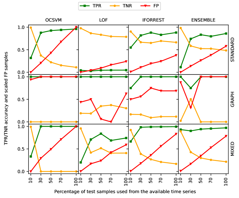
Figure 2: Test results for the models from Table I on the UNSW-NB15 dataset. For graphical purposes, for each row the number of false positives (FP) are scaled in the $[0,1]$ interval.

We now use the models form Table I as predictors for the rest of the data samples from the UNSW-NB15 dataset. Figure 2 depicts the performance for different test dataset sizes: 10%, 30%, 50%, 70% and 100%. The True Positive Rates (TPR) and True Negative Rates (TNR) are analyzed together with the number of False Positives (FP) for all models, depicted on the columns, and for all approaches, depicted on the rows. For each row, the number of false positives were scaled such that the reader can see the relative differences between each method. As expected, model performance degrades with time as normal behaviour evolves and new types of attacks arrive. We observe that OC-SVM is the most sensible to these changes, while IForest seems more robust. Ensembles tend to attenuate false positives and promote good TPR rates.

V Conclusions

In this paper we studied the performance of unsupervised machine learning methods when analyzing computer networks by starting from a small dataset of known labeled packet samples that we use to tune model parametrization which we then use to investigate their performance for further unsupervised learning on new incoming unlabeled data. Data is augmented through graph feature extraction techniques, such as egonets and random walks, in order to improve the robustness of our models.

References

- [1] CyberEdge. 2021 cyberthreat defense report. https://cyber-edge.com/wp-content/uploads/2021/04/CyberEdge-2021-CDR-Report-v1.1-1.pdf, 2021.
- [2] Peter J Huber. Robust statistics, volume 523. John Wiley & Sons, 2004.
- [3] Koral Ilgun, Richard A Kemmerer, and Phillip A Porras. State transition analysis: A rule-based intrusion detection approach. IEEE transactions on software engineering, 21(3):181–199, 1995.
- [4] Kenji Yamanishi and Jun-ichi Takeuchi. Discovering outlier filtering rules from unlabeled data: combining a supervised learner with an unsupervised learner. In Proceedings of the seventh ACM SIGKDD international conference on Knowledge discovery and data mining, pages 389–394, 2001.
- [5] Robert Gwadera, Mikhail Atallah, and Wojciech Szpankowski. Markov models for identification of significant episodes. In Proceedings of the 2005 SIAM international conference on data mining, pages 404–414. SIAM, 2005.
- [6] Dit-Yan Yeung and Calvin Chow. Parzen-window network intrusion detectors. In Object recognition supported by user interaction for service robots, volume 4, pages 385–388. IEEE, 2002.
- [7] Sunanda Gamage and Jagath Samarabandu. Deep learning methods in network intrusion detection: A survey and an objective comparison. Journal of Network and Computer Applications, 169:102767, 2020.
- [8] Dylan Chou and Meng Jiang. A survey on data-driven network intrusion detection. ACM Computing Surveys (CSUR), 54(9):1–36, 2021.
- [9] Zeeshan Ahmad, Adnan Shahid Khan, Cheah Wai Shiang, Johari Abdullah, and Farhan Ahmad. Network intrusion detection system: A systematic study of machine learning and deep learning approaches. Transactions on Emerging Telecommunications Technologies, 32(1):e4150, 2021.
- [10] Chuanlong Yin, Yuefei Zhu, Jinlong Fei, and Xinzheng He. A deep learning approach for intrusion detection using recurrent neural networks. Ieee Access, 5:21954–21961, 2017.
- [11] Nico Görnitz, Marius Kloft, Konrad Rieck, and Ulf Brefeld. Active learning for network intrusion detection. In Proceedings of the 2nd ACM workshop on Security and artificial intelligence, pages 47–54, 2009.
- [12] Roberto Perdisci, Guofei Gu, and Wenke Lee. Using an ensemble of one-class svm classifiers to harden payload-based anomaly detection systems. In Sixth International Conference on Data Mining (ICDM’06), pages 488–498. IEEE, 2006.
- [13] K Keerthi Vasan and B Surendiran. Dimensionality reduction using principal component analysis for network intrusion detection. Perspectives in Science, 8:510–512, 2016.
- [14] Mei-Ling Shyu, Shu-Ching Chen, Kanoksri Sarinnapakorn, and LiWu Chang. A novel anomaly detection scheme based on principal component classifier. Technical report, Miami Univ Coral Gables Fl Dept of Electrical and Computer Engineering, 2003.
- [15] Mariam Kiran, Cong Wang, George Papadimitriou, Anirban Mandal, and Ewa Deelman. Detecting anomalous packets in network transfers: investigations using pca, autoencoder and isolation forest in tcp. Machine Learning, 109(5):1127–1143, 2020.
- [16] Mohiuddin Ahmed. Collective anomaly detection techniques for network traffic analysis. Annals of data science, 5(4):497–512, 2018.
- [17] Haipeng Yao, Danyang Fu, Peiying Zhang, Maozhen Li, and Yunjie Liu. Msml: A novel multilevel semi-supervised machine learning framework for intrusion detection system. IEEE Internet of Things Journal, 6(2):1949–1959, 2018.
- [18] Leman Akoglu, Hanghang Tong, and Danai Koutra. Graph based anomaly detection and description: a survey. Data mining and knowledge discovery, 29(3):626–688, 2015.
- [19] Weisong He, Guangmin Hu, and Yingjie Zhou. Large-scale ip network behavior anomaly detection and identification using substructure-based approach and multivariate time series mining. Telecommunication Systems, 50(1):1–13, 2012.
- [20] Pin-Yu Chen, Sutanay Choudhury, and Alfred O Hero. Multi-centrality graph spectral decompositions and their application to cyber intrusion detection. In 2016 IEEE International Conference on Acoustics, Speech and Signal Processing (ICASSP), pages 4553–4557. IEEE, 2016.
- [21] Frank Capobianco, Rahul George, Kaiming Huang, Trent Jaeger, Srikanth Krishnamurthy, Zhiyun Qian, Mathias Payer, and Paul Yu. Employing attack graphs for intrusion detection. In Proceedings of the New Security Paradigms Workshop, pages 16–30, 2019.
- [22] Qingsai Xiao, Jian Liu, Quiyun Wang, Zhengwei Jiang, Xuren Wang, and Yepeng Yao. Towards network anomaly detection using graph embedding. In International Conference on Computational Science, pages 156–169. Springer, 2020.
- [23] Paul Irofti, Ștefania Budulan, Bogdan Dumitrescu, and Andra Băltoiu. Graphomaly’s official documentation. https://unibuc.gitlab.io/graphomaly/graphomaly, 2022. Accessed: 2022-05-14.
- [24] Markus M Breunig, Hans-Peter Kriegel, Raymond T Ng, and Jörg Sander. Lof: identifying density-based local outliers. In Proceedings of the 2000 ACM SIGMOD international conference on Management of data, pages 93–104, 2000.
- [25] Fei Tony Liu, Kai Ming Ting, and Zhi-Hua Zhou. Isolation forest. In 2008 eighth ieee international conference on data mining, pages 413–422. IEEE, 2008.
- [26] Yue Zhao, Zain Nasrullah, Maciej K Hryniewicki, and Zheng Li. Lscp: Locally selective combination in parallel outlier ensembles. In Proceedings of the 2019 SIAM International Conference on Data Mining, pages 585–593. SIAM, 2019.
- [27] Charu C Aggarwal and Saket Sathe. Theoretical foundations and algorithms for outlier ensembles. Acm sigkdd explorations newsletter, 17(1):24–47, 2015.
- [28] Zheng Li Yue Zhao, Zain Nasrullah. Pyod: A python toolbox for scalable outlier detection. Journal of Machine Learning Research (JMLR), pages 1–7, 2019.