Field-Induced Quantum Spin Nematic Liquid Phase in the S=1 Antiferromagnetic Heisenberg Chain with Additional Interactions

Abstract

The magnetization process of the $S=1$ antiferromagnetic chain with the single-ion anisotropy $D$ and the biquadratic interaction is investigated using the numerical diagonalization. Both interactions stabilize the 2-magnon Tomonaga-Luttinger liquid (TLL) phase in the magnetization process. Based on several excitation gaps calculated by the numerical diagonalization, some phase diagrams of the magnetization process are presented. These phase diagrams reveal that the spin nematic dominant TLL phase appears at higher magnetizations for sufficiently large negative $D$.

1 Introduction

The quantum spin nematic state is one of interesting topics in the field of the strongly correlated electron systems. It was theoretically predicted to be realized in several frustrated systems; the square-lattice model with the ferromagnetic nearest-neighbor and antiferromagnetic next-nearest-neighbor interactions[1], the triangular-lattice antiferromagnetic with multi spin exchange interactions[2], and the ferromagnetic and antiferromagnetic zigzag chain[3, 4]. The high-magnetic field measurement[5] on the zigzag chain compound LiCuVO₄ detected an anomalous behavior of the magnetization curve just below the saturation magnetization, which was supposed to be the spin nematic phase. The quantum spin liquid like behavior of the $S=1$ triangular-lattice compound NiGa₂S₄ was theoretically explained as the spin nematic state[6]. A density matrix renormalization group (DMRG) analysis[7] indicated that the field-induced spin nematic liquid phase appears in the $S=1$ antiferromagnetic chain with the biquadratic interaction. It was supported by the numerical diagonalization study[8].

On the other hand, the 2-magnon bound state similar to the spin nematic state was predicted to appear in the magnetization process of the $S=1$ antiferromagnetic chain with the easy axis anisotropy based on the numerical diagonalization analysis[9]. It would possibly correspond to the spin nematic state. In the present paper, we investigate the $S=1$ antiferromagnetic chain with the easy axis anisotropy and the biquadratic interaction using the numerical diagonalization, in order to consider the relation between this 2-magnon bound state and the spin nematic liquid phase.

2 Model

We consider the magnetization process of the $S=1$ antiferromagnetic chain with the easy axis single ion anisotropy $D$ and the biquadratic interaction $J_{\rm BQ}$. The system under the magnetic field is described by the Hamiltonian

$${\cal H} = {\cal H}_{0}+{\cal H}_{Z}$$ (1)

$${\cal H}_{0} = J\sum_{j=1}^{L}\vec{S}_{j}\cdot\vec{S}_{j+1}+D\sum_{j=1}^{L}(S_{j}^{z})^{2}+J_{\rm BQ}\sum_{j=1}^{L}(\vec{S}_{j}\cdot\vec{S}_{j+1})^{2}$$ (2)

$${\cal H}_{Z} = -H\sum_{j=1}^{L}S_{j}^{z}.$$ (3)

In this paper we consider the case of $J_{\rm BQ}<0$, $D<0$ and fix $J=1$. The first term of ${\cal H}_{0}$ is the bilinear exchange interaction which stabilizes the antiparallel configuration of the nearest neighbor spin pair. On the other hand, the third term, the biquadratic interaction does not only stabilize the antiparallel configuration, but also the parallel one. Thus the spin nematic liquid phase would possibly occur for sufficiently large $|J_{\rm BQ}|$. A numerical diagonalization and DMRG study indicated that the biquadratic interaction stabilizes the spin nematic correlation[10]. If the spin nematic liquid phase is realized, the four spin correlation function would exhibit the power-law decay, while the two spin one decays exponentially. Then in this phase the single magnon excitation should be gapped, but the 2-magnon excitation should be gapless. Therefore the 2-magnon bound state would be realized there. If the spin nematic liquid phase appears in the magnetization process described by the Hamiltonian (3), each step of the magnetization curve for the finite-size systems should be $\delta S^{z}_{\rm total}=2$, while $\delta S^{z}_{\rm total}=1$ in the conventional Tomonaga-Luttinger liquid (TLL) phase. The negative $D$ also yields a similar 2-magnon bound state, because the $S_{j}^{z}=\pm 1$ states are stabilized and the $S_{j}^{z}=0$ state is skipped[9]. In order to clarify the feature of these 2-magnon bound states, we investigate the model (3) using the numerical diagonalization of finite clusters under the periodic boundary condition. The calculated lowest energy for each magnetization $M=(\sum_{j=1}^{L}S_{j}^{z})$ and each momentum $k$ is denoted as $E_{k}(M)$ in the following sections.

3 Spin Nematic Liquid

The negative biquadratic interaction stabilizes the TLL phase where the 2-magnon bound state is realized, as well as the negative $D$. In this 2-magnon TLL phase the spin correlation functions are expected to have the following asymptotic forms:

$$\langle(S_{0}^{+})^{2}(S_{r}^{-})^{2}\rangle\sim r^{-{\eta}_{2}},\quad\langle S_{0}^{z}S_{r}^{z}\rangle\sim\cos(2k_{F}r)r^{-{\eta}_{z}}\quad(r\rightarrow\infty),$$ (4)

where $2k_{F}$ is given by $2k_{F}=(1-M/M_{s})\pi$ and $M_{s}$ is the saturation magnetization ($M_{s}=L$). $\langle(S_{0}^{+})^{2}(S_{r}^{-})^{2}\rangle$ is the nematic (quadrapole) correlation perpendicular to the magnetic field and $\langle S_{0}^{z}S_{r}^{z}\rangle$ is the SDW correlation parallel to it. In a DMRG work[7] the region with ${\eta}_{2}<{\eta}_{z}$ is called the nematic phase and the region with ${\eta}_{2}>{\eta}_{z}$ is called the SDW phase, although the boundary between them is just a crossover line. Thus in order to find the spin nematic liquid phase, we should look for the parameter region where the 2-magnon TLL is realized and ${\eta}_{2}<{\eta}_{z}$ is satisfied.

4 Exciation Gaps

In order to determine the boundary between the 1-magnon (conventional) and 2-magnon TLL phases, we consider several excitation gaps. The 2-magnon excitation gap $\Delta_{2}$ is gapless in both phases. The 1-magnon excitation gap $\Delta_{1}$ (the $2k_{F}$ excitation gap of the 2-magnons $\Delta_{2k_{F}}$) is gapless (gapped ) in the 1-magnon TLL phase, while gapped (gapless) in the 2-magnon one. $D$ dependence of the scaled excitation gaps $L\Delta_{1}$, $L\Delta_{2}$ and $L\Delta_{2k_{F}}$ at $M=M_{s}/2$ for $J_{\rm BQ}=-0.2$ are shown in Fig. 1(a). Fig. 1(a) indicates the above behaviors of these gaps. The cross point of $\Delta_{1}$ and $\Delta_{2k_{F}}$ is one of good estimations of the phase boundary between the 1-magon and 2-magon TLL phases. Our analysis of the $L$ dependence indicates that this phase boundary converges faster than $1/L^{2}$ with respect to $L$. Thus we adopt this method to determine the boundary between the 1-magnon and 2-magnon TLL phases.

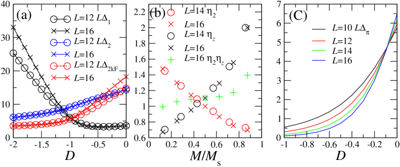
Figure 1: (a)Scaled gaps $L\Delta_{1}$, $L\Delta_{2}$ and $L\Delta_{2k_{F}}$ at $M=M_{s}/2$ for $J_{\rm BQ}$=-0.2 are plotted versus $D$ for $L=12$ and 16, (b)Exponents $\eta_{2}$ and $\eta_{z}$ estimated by (5) plotted versus $M/M_{s}$ for $L=$14 and 16 ($J_{\rm BQ}$=-0.2, $D$=-1.5). $\eta_{2}\eta_{z}=1$ is well satisfied around the cross of $\eta_{2}$ and $\eta_{z}$. (c)Scaled gaps $L\Delta_{\pi}$ for $J_{\rm BQ}=-0.2$. It indicates the phase boundary about $D\sim-0.1$.

5 Spin Correlation Exponents

According to the conformal field theory, the critical exponents $\eta_{2}$ and $\eta_{z}$ can be estimated the forms

$$\eta_{2}={{E_{0}(M+2)+E_{0}(M-2)-2E_{0}(M)}\over{E_{k_{1}}(M)-E_{0}(M)}},\quad\eta_{z}=2{{E_{2k_{F}}(M)-E_{0}(M)}\over{E_{k_{1}}(M)-E_{0}(M)}},$$ (5)

for each magnetization $M$, where $k_{1}$ is defined as $k_{1}=L/2\pi$. $\eta_{2}$ and $\eta_{z}$ estimated for $L$=14 and 16 are plotted versus $M/M_{s}$ in Fig. 1 (b). It suggests that the SDW correlation is dominant for small $M$, while the nematic one is for large $M$. Since the cross point of $\eta_{2}$ and $\eta_{z}$ is not so strongly dependent of $L$, the cross point of $L=16$ is used as the crossover point between the SDW and nematic TLL phases in Fig. 2(a), (b) and (c), for $J_{\rm BQ}$=0, -0.2 and -0.5, respectively. At least around the cross point the system well holds the relation $\eta_{2}\eta_{z}=1$, which should be satisfied for TLL, as shown in Fig. 1(b).

6 Phase diagrams

The phase diagrams on the $D$-$M/M_{s}$ plane are presented for $J_{\rm BQ}$=0, -0.2, and -0.5 in Figs. 2 (a), (b), and (c), respectively. The phase boundary at $M=0$ between the Haldane and Néel ordered phases, which is denoted as the green triangle in Fig. 2, is determined by the phenomenological renormalization using the excitation gap $\Delta_{\pi}$ with $k=\pi$ for $L$=10, 12, 14, and 16. The scaled gap $L\Delta_{\pi}$ is plotted versus $D$ for $J_{\rm BQ}=-0.2$ in Fig. 1(c). The $L$ dependent critical point obtained by $L\Delta_{\pi}(L,D_{c})=(L+2)\Delta_{\pi}(L+2,D_{c})$ can be easily extrapolated to the infinite $L$ limit. The critical point at $M=M_{s}$ is determined as the point where the 1-magnon and 2-magnon excitation gaps are equal, which is the blue triangle in Fig. 2. Here, NTLL, SDWTLL and CTLL denote the nematic TLL, the SDW TLL, and the conventional TLL, respectively. Fig.2(a) indicates that the NTLL can appear even for $J_{\rm BQ}=0$. Figs. 2(b) and (c) suggest that the biquadratic interaction enhances both of NTLL and SDWTLL phases. The crossover boundary between NTLL and SDWTLL is always about the half the saturation magnetization. It is not so strongly dependent on $J_{\rm BQ}$.

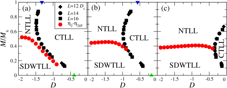
Figure 2: Phase diagrams with respect to $D$ and $M/M_{s}$ for $J_{\rm BQ}$=0(a), -0.2(b) and -0.5(c).

7 Summary

The magnetization process of the $S=1$ antiferromagnetic chain with the easy-axis single-ion anisotropy and the biquadratic interaction is investigated by the numerical diagonalization for finite-size systems. It is found that the nematic TLL phase appears in higher magnetization region for sufficiently large negative $D$, even for $J_{\rm BQ}=0$.

References

References

- [1] N. Shannon, T. Momoi and P. Sindzingre, Phys. Rev. Lett. 96, 027213 (2006).
- [2] T. Momoi, P. Sindzingre and N. Shannon, Phys. Rev. Lett. 97, 257204 (2006).
- [3] A. V. Chubukov, Phys. Rev. B 44, R4693 (1991).
- [4] T. Hikihara, L. Kecke, T. Momoi and A. Furusaki, Phys. Rev. B 78, 144404 (2008).
- [5] N. Büttgen et al., Phys. Rev. B 90, 134401 (2014).
- [6] S. Nakatsuji et al., Science 309, 1697 (2005).
- [7] S. R. Manmana, A. M, Lauchli, F. H. L. Essler and F. Mila, Phys. Rev. B 83, 184433 (2011).
- [8] T. Sakai, AIP Advances 11, 015306 (2021).
- [9] T. Sakai, Phys. Rev. B 58, 6268 (1998).
- [10] A. Lauchli, G. Schmid and S. Trebst, Phys. Rev. B 74, 144426 (2006).