Naturalistic Causal Probing for Morpho-Syntax

Abstract

Probing has become a go-to methodology for interpreting and analyzing deep neural models in natural language processing. However, there is still a lack of understanding of the limitations and weaknesses of various types of probes. In this work, we suggest a strategy for input-level intervention on naturalistic sentences. Using our approach, we intervene on the morpho-syntactic features of a sentence, while keeping the rest of the sentence unchanged. Such an intervention allows us to causally probe pre-trained models. We apply our naturalistic causal probing framework to analyze the effects of grammatical gender and number on contextualized representations extracted from three pre-trained models in Spanish: the multilingual versions of BERT, RoBERTa, and GPT-2. Our experiments suggest that naturalistic interventions lead to stable estimates of the causal effects of various linguistic properties. Moreover, our experiments demonstrate the importance of naturalistic causal probing when analyzing pre-trained models.

https://github.com/rycolab/naturalistic-causal-probing

1 Introduction

Contextualized word representations are a byproduct of pre-trained neural language models and have led to improvements in performance on a myriad of downstream natural language processing (NLP) tasks (Joshi et al., 2019; Kondratyuk, 2019; Zellers et al., 2019; Brown et al., 2020). Despite this performance improvement, though, it is still not obvious to researchers how these representations encode linguistic information. One prominent line of work attempts to shed light on this topic through probing (Alain and Bengio, 2017), also referred to as auxiliary prediction Adi et al. (2017) or diagnostic classification Hupkes et al. (2018). In machine learning parlance, a probe is a supervised classifier that is trained to predict a property of interest from the target model’s representations. If the probe manages to predict the property with high accuracy, one may conclude that these representations encode information about the probed property.

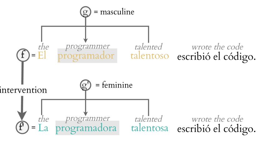
Figure 1: Intervention on the gender of lemma programador (masculine $\rightarrow$ feminine). Changes are propagated from that noun to its dependent words accordingly.

While widely used, probing is not without its limitations. For instance, probing a pre-trained model for grammatical gender can only tell us whether information about gender is present in the representations, it cannot, however, tell us how or if the model actually uses information about gender in its predictions (Ravichander et al., 2021; Elazar et al., 2021; Ravfogel et al., 2021; Lasri et al., 2022). Furthermore, supervised probing cannot tell us whether the property under consideration is directly encoded in the representations, or if it can be recovered from the representations alone due to spurious correlations among various linguistic properties. In other words, while through supervised probing techniques we might find correlations between a probed property and representations, we cannot uncover causal relationships between them.

In this work, we propose a new strategy for input-level intervention on naturalistic data to obtain what we call naturalistic counterfactuals, which we then use to perform causal probing. Through such input-level interventions, we can ascertain whether a particular linguistic property has a causal effect on a model’s representations. A number of prior papers have attempted to tease apart causal dependencies using either input-level or representation-level interventions. For instance, work on representational counterfactuals has investigated causal dependencies via interventions on neural representations. While quite versatile, representation-level interventions make it hard—if not impossible—to determine whether we are only intervening on our property of interest. Another proposed method, templated counterfactuals, does perform an input-level intervention strategy, ensuring that only the probed property will be affected. Under such an approach, the researcher first creates a number of templated sentences (either manually or automatically), which they then fill with a set of minimal-pair words to generate counterfactual examples. However, template-based interventions are limited by design: They do not reflect the diversity of sentences present in natural language, and, thus, lead to biased estimates of the measured causal effects. Naturalistic counterfactuals improve upon template-based interventions in that they lead to unbiased estimates of the causal effect.

In our first set of experiments, we employ naturalistic causal probing to estimate the average treatment effect (ATE) of two morpho-syntactic features—namely, number and grammatical gender—on a noun’s contextualized representation. We show the estimated ATE’s stability across corpora. In our second set of experiments, we find that a noun’s grammatical gender and its number are encoded by a small number of directions in three pre-trained models’ representations: BERT, RoBERTa, and GPT-2. We further use naturalistic counterfactuals to causally investigate gender bias in RoBERTa. We find that RoBERTa is much more likely to predict the adjective hermoso(a) (beautiful) for feminine nouns and racional (rational) for masculine. This suggests RoBERTa is indeed gender biased in its adjective predictions.

Finally, through our naturalistic counterfactuals, we show that correlational probes overestimate the presence of certain linguistic properties. We compare the performance of correlational probes on two versions of our dataset: one unaltered and one augmented with naturalistic counterfactuals. While correlational probes achieve very high (above 90%) performance when predicting gender from sentence-level representations, they only perform close to chance (around 60%) on the augmented data. Together, our results demonstrate the importance of a naturalistic causal approach to probing.

2 Probing

There are several types of probing methods that have been proposed for the analysis of NLP models, and there are many possible taxonomies of those methods. For the purposes of this paper, we divide previously proposed probing models into two groups: correlational and causal probes. On one hand, correlational probes attempt to uncover whether a probed property is present in a model’s representations. On the other hand, causal probes, roughly speaking, attempt to uncover how a model encodes and makes use of a specific probed property. We compare and contrast correlational and causal probing techniques in this section.

2.1 Correlational Probing

Correlational probing is any attempt to correlate the input representations with the probed property of interest. Under correlational probing, the performance of a probe is viewed as the degree to which a model encodes information in its representations about some probed property (Alain and Bengio, 2017). At various times, correlational results have been used to claim that language models have knowledge of various morphological, syntactic, and semantic phenomena (Adi et al., 2017; Ettinger et al., 2016; Belinkov et al., 2017; Conneau et al., 2018, inter alia). Yet the validity of these claims has been a subject of debate (Saphra and Lopez, 2019; Hewitt and Liang, 2019; Pimentel et al., 2020a, b; Voita and Titov, 2020).

2.2 Causal Probing

A more recent line of work aims to answer the question: What is the causal relationship between the property of interest and the probed model’s representations? In natural language, however, answering this question is not straightforward: sentences typically contain confounding factors that render analyses tedious. To circumvent this problem, most work in causal probing relies on interventions, i.e., the act of setting a variable of interest to a fixed value (Pearl, 2009). Importantly, this must be done without altering any of this variable’s causal parents, thereby keeping their probability distributions fixed. As a byproduct, these interventions generate counterfactuals, i.e., examples where a specific property of interest is changed while everything else is held constant. Counterfactuals can then be used to perform a causal analysis. Prior probing papers have proposed methods using both representational and templated counterfactuals, as we discuss next.

Representational Counterfactuals.

A few recent causal probing papers perform interventions directly on a model’s representations (Giulianelli et al., 2018; Feder et al., 2021; Vig et al., 2020; Tucker et al., 2021; Ravfogel et al., 2021; Lasri et al., 2022; Ravfogel et al., 2022a). For example, Elazar et al. (2021) use iterative null space projection (INLP; Ravfogel et al., 2020) to remove an analyzed property’s information, e.g., part of speech, from the representations. Although representational interventions can be applied to situations where other forms of intervention are not feasible, it is often impossible to make sure only the information about the probed property is removed or changed. In the absence of this guarantee, any causal conclusion should be viewed with caution.

Templated Counterfactuals.

Other works (Vig et al., 2020; Finlayson et al., 2021), like us, have leveraged input-level interventions. However, in these cases, the interventions are carried out using templated minimal-pair sentences, which differ only with respect to a single analyzed property. Using these minimal pairs, they estimate the effect of an input-level intervention on individual attention heads and neurons. One benefit of template-based approaches is that they create a highly controlled environment, which guarantees that the intervention is done correctly, and which may lead to insights that would be impossible to gain from natural data. However, since the templates are typically designed to analyze a specific property, they cover a narrow set linguistic phenomena, which may not reflect the complexity of language in naturalistic data.

Naturalistic Counterfactuals.

In this paper, following Zmigrod et al. (2019), we propose a new and less complex strategy to perform input-level interventions by creating naturalistic counterfactuals that are not derived from templates. Instead, we derive the counterfactuals from the dependency structure of the sentence. By creating counterfactuals on the fly using a dependency parse, we avoid the biases of manually creating templates. Furthermore, our approach guarantees that we only intervene on the specific linguistic property of interest, e.g., changing the grammatical gender or number of a noun.

3 The Causal Framework

The question of interest in this paper is how contextualized representations are causally affected by a morpho-syntactic feature such as gender or number. To see how our method works, it is easiest to start with an example. Let’s consider the following pair of Spanish sentences:

. El programador talentoso escribió el código.
the.m.sg programmer.m.sg talented.m.sg wrote the code.
The talented programmer wrote the code.

. La programadora talentosa escribió el código.
the.f.sg programmer.f.sg talented.f.sg wrote the code.
The talented programmer wrote the code.

The meaning of these sentences is equivalent up to the gender of the noun programador, whose feminine form is programadora. However, more than just this one word changes from 3 to 3: The definite article el changes to la and the adjective talentoso changes to talentosa. In the terminology of this paper, we will refer to programador as the focus noun, as it is the noun whose grammatical properties we are going to change. We will refer to the changing of 3 to 3 as a syntactic intervention on the focus noun. Informally, a syntactic intervention may be thought of as taking part in two steps. First, we swap the focus noun (programador) with another noun that is equivalent up to a single grammatical property. In this case, we swap programador with programadora which differs only in its gender marking. Second, we reinflect the sentence so that all necessary words grammatically agree with the new focus noun. The result of a syntactic intervention is a pair of sentences that differ minimally, i.e., only with respect to this one grammatical property. Another way of framing the syntactic intervention is as a counterfactual: What would 3 have looked like if programador had been feminine? The rest of this section focuses on formalizing the notion of a syntactic intervention and discussing how to use them in a causal inference framework for probing.

A Note on Inanimate Nouns.

When estimating the effect of grammatical gender here, we restrict our investigation to animate nouns, e.g., programadora/programador (feminine/masculine programmer). Grammatical gender of inanimate nouns is lexicalized, meaning that each noun is assigned a single gender, e.g., puente (bridge) is masculine. In other words, there is not a non-zero probability of assigning each lemmata to each gender, which violates a condition called positivity in causal inference literature. Thus, we cannot perform an intervention on the grammatical gender of those words, but rather would need to perform an intervention on the lemma itself. We refer to Gonen et al. (2019) for an analysis of the effect of gender on inanimate nouns’ representations. Note that a similar lexicalization can also be observed in a few animate nouns, e.g. madre/padre (mother/father). In such cases, to separate the lemma from gender, we assume that these words share a hypothetical lemma, which in our example represents parenthood, and combining that with gender would give us the specific forms, e.g. madre/padre.

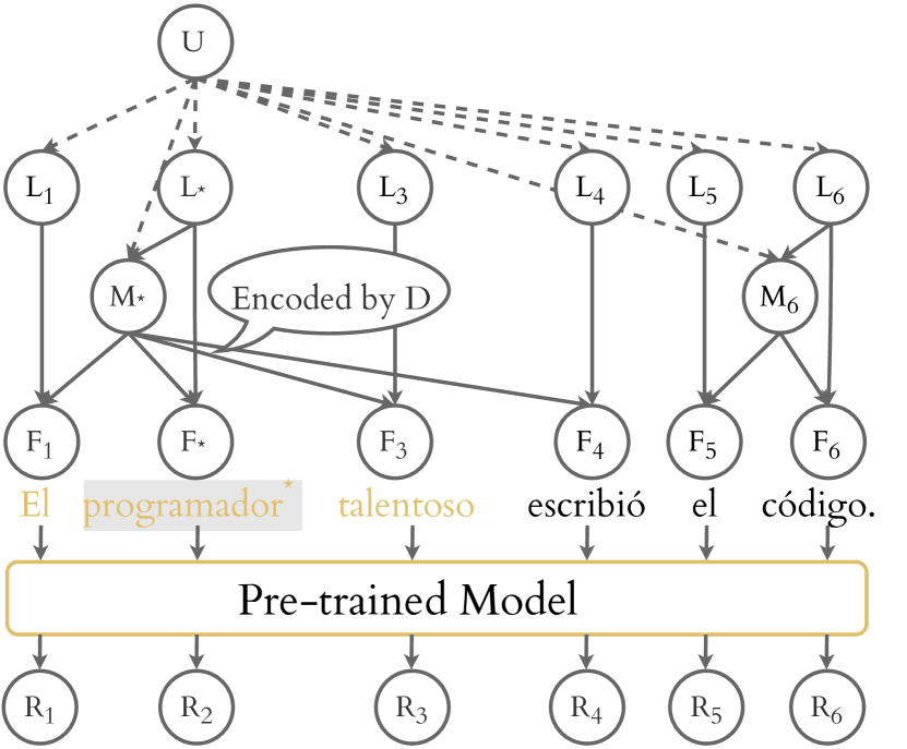
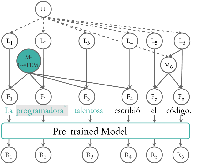
Figure 2: Causal graph for the Spanish sentence El programador talentoso escribió el código. before (on the left) and after (on the right) an intervention on the grammatical gender of the focus noun.

3.1 The Causal Model

We now describe a causal model that will allow us to more formally discuss syntactic interventions.

Notation and Variables.

We denote random variables in upper-case letters and instances with lower-case letters. We bold sequences: bold lower-case letters represent a sequence of words and bold upper-case letters represent a sequence of random variables. Let $\boldsymbol{f}=\langle f_{1},\ldots,f_{T}\rangle$ be a sentence (of length $T$) where each $f_{t}$ is a word form. In addition, let $\mathbf{r}$ be the list of contextual representations $\mathbf{r}=\langle r_{1},\ldots,r_{T}\rangle$ where each $r_{t}\in\mathbb{R}^{h}$, and is in one-to-one correspondence with the sentence $\boldsymbol{f}$, i.e., $r_{t}$ is $f_{t}$’s contextual representation. Furthermore, let $\boldsymbol{\ell}=\langle\ell_{1},\ldots,\ell_{T}\rangle$ be a list of lemmata and $\widetilde{\boldsymbol{m}}=\langle m_{1},\ldots,m_{T}\rangle$ a list of morpho-syntactic features co-indexed with $\boldsymbol{f}$; $\ell_{t}$ is the lemma of $f_{t}$ and $m_{t}$ is its morpho-syntactic features. We call $\boldsymbol{m}=\langle m_{t_{1}},\ldots,m_{t_{K}}\rangle$ the minimal list of morpho-syntactic features, where each $t_{k}$ is an index between 1 to $T$. In essence, we drop features of the tokens that are dependent on other tokens’ morphology. In our example 3 this means we only include the morpho-syntactic features of programador and código, thus $\boldsymbol{m}=\langle m_{2},m_{6}\rangle$. We denote the morpho-syntactic feature of interest as $m_{*}$, which, in this work, represents either the gender $g_{*}$ or number $n_{*}$ of the focus noun. We further denote the lemma of the focus noun as $\ell_{*}$.

Causal Assumptions.

Our causal model is introduced in Fig. 2. It encodes the causal relationships between $U,\boldsymbol{L},\boldsymbol{M},\boldsymbol{F}$ and $\mathbf{R}$. Explicitly, we assume the following causal relationships:

• $\boldsymbol{M}$ and $\boldsymbol{L}$ are causally dependent on $U$. The underlying meaning that the writer of a sentence wants to convey determines the used lemmas and morpho-syntactic features;

• In general, $L_{t}$ can causally affect $M_{t}$. Take the gender of inanimate nouns as an example, where the lemma determines the gender;

• $\boldsymbol{F}$ is causally dependent on $\boldsymbol{L}$ and $\boldsymbol{M}$. Word forms are a combination of lemmata and morpho-syntactic features;

• $\mathbf{R}$ is causally dependent on $\boldsymbol{F}$. Contextualized representations are obtained by processing the sentences through the probed model.

Dependency Trees.

In order to measure the causal effect of the gender of the focus noun ($g_{*}$) on the contextualized representation ($\mathbf{r}$), all of its causal dependencies must be considered. As our causal graph shows (in Fig. 2), $g_{*}$ not only has a causal effect on the focus noun’s form, but also on the definite article el and the adjective talentoso. Yet, not all word forms in a sentence are affected; for instance, the definite article el in the noun phrase el código. Luckily, within a given sentence, such relationships are naturally encoded by that sentence’s dependency tree. The dependency graph $d$ of a sentence $\boldsymbol{f}$ is a directed graph created by connecting each word form $f_{t}$ for $1\leq t\leq T$ to its syntactic parent. We use the information encoded in $d$ by leveraging the fact that a word form $f_{t}$ is causally dependent on its syntactic parent. In essence, a dependency tree $d$ implicitly encodes a function $d_{t}[\boldsymbol{m}]$ which returns the subset of morphological properties that causally affect the form $f_{t}$. Thus, we are able to express the complete joint probability distribution of our causal model as follows:

$$p(\boldsymbol{f},\boldsymbol{m} ,\boldsymbol{\ell},u)$$ (1)

$$=p(u)\,p(\boldsymbol{m},\boldsymbol{\ell}\mid u)\,p(\boldsymbol{f}\mid\boldsymbol{m},\boldsymbol{\ell})$$

$$=p(u)\,p(\boldsymbol{m},\boldsymbol{\ell}\mid u)\,\prod_{t=1}^{T}p(f_{t}\mid d_{t}[\boldsymbol{m}],\ell_{t})$$

Abstract Causal Model.

We can now simplify the causal model from Fig. 2 into Fig. 3. For simplicity, we isolate the lemma and morpho-syntactic feature of interest $L_{*}$ and $M_{*}$ and aggregate the other lemmata and morpho-syntactic features into an abstract variable, which we call $\boldsymbol{Z}$ and refer to as the context. Furthermore, we only show the aggregation of word forms and representations as $\boldsymbol{F}$ and $\mathbf{R}$ in the abstract model. We will assume for now, and in most of our experiments, that the output of the causal model ($\mathbf{R}$ in Fig. 3) represents the contextualized representation of the focus noun. However, as we generalize later, the output of the causal model can be any function of word forms $\boldsymbol{F}$, such as: the representation of other words in the sentence, the probability distribution assigned by the model to a masked word, or even the output of a downstream task. We note that Fig. 3 can be easily re-expanded into Fig. 2 for any specific utterance by using its dependency tree.

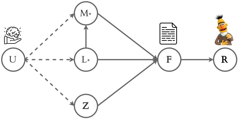
Figure 3: Causal model showing dependencies between the underlying meaning ($U$), lemma ($L_{*}$) and morpho-syntactic features ($M_{*}$) of the focus noun, context ($\boldsymbol{Z}$), sentences ($\boldsymbol{F}$) and contextualized representations ($\mathbf{R}$).

3.2 Naturalistic Counterfactuals

In causal inference literature, the $\mathrm{do}(\cdot)$ operator represents an intervention on a causal diagram. For instance, we might want to intervene on the gender of the focus noun (thus using gender $G_{*}$ as the morpho-syntactic feature of interest $M_{*}$). Concretely, in our example (Fig. 2), $\mathrm{do}(G_{*}=\textsc{fem})$ means intervening on the causal graph by removing all the causal edges going into $G_{*}$ from $U$ and $L_{*}$ and setting $G_{*}$’s value to a specific realization fem. The result of this intervention on a sampled sentence $\boldsymbol{f}$ is a new counterfactual sentence $\boldsymbol{f}^{\prime}$. As our causal graph suggests, the relationship between words in a sentence is complex, occurring at multiple levels of abstraction; swapping the gender of a single word—while leaving all other words unchanged—may not result in grammatical text. Consequently, one must approach the creation of counterfactuals in natural language with caution. Specifically, we rely on syntactic interventions to generate our naturalistic counterfactuals.

Syntactic Intervention.

We develop a heuristic algorithm to perform our interventions, shown in App. B. Given a sentence and its dependency tree, the algorithm generates a counterfactual version of the sentence, i.e., approximating the $\mathrm{do}(\cdot)$ operation. This algorithm processes the dependency tree of each sentence in a depth-first search recursive manner. In each iteration, if the node in process is a noun, it is marked as the focus noun and a new copy of the sentence is created, which will be the base of the counterfactual sentence. Then, the intervention is performed, altering the focus noun and all dependent tokens in the copied sentence. Notedly, when we syntactically intervene on the grammatical gender or number of a noun, we do not alter potentially incompatible semantic contexts. Take sentence 3.2 as an example, where the focus noun is mujer and we intervene on gender. Its counterfactual sentence 3.2 is semantically odd and unlikely, but still meaningful. We can thus estimate the causal effect of grammatical gender in the contextual representations—breaking the correlation between morpho-syntax and semantics.

. La mujer dio a luz a 6 bebés.
the.f.sg woman.f.sg gave birth to 6 babies.
The woman gave birth to 6 babies.

. El hombre dio a luz a 6 bebés.
the.m.sg man.m.sg gave birth to 6 babies.
The man gave birth to 6 babies.

3.3 Measuring Causal Effects

In this section, we define the causal effect of a morpho-syntactic feature. We then present estimators for these values in the following section. While we focus on grammatical gender here, our derivations are similarly applicable to number and other morpho-syntactic features.

Given a specific focus–context pair $(\ell_{*},\boldsymbol{z})$, the causal effect of gender $G_{*}$ on the representations is called the individual treatment effect (ITE; Rosenbaum and Rubin, 1983) and is defined as:

$$\Delta(\ell_{*},\boldsymbol{z})=$$ (2)

$$\quad\operatorname*{\mathbb{E}}_{\boldsymbol{F}}\Big{[}\mathtt{tgt}(\boldsymbol{F})\mid G_{*}\!=\!\textsc{msc},L_{*}\!=\!\ell_{*},\boldsymbol{Z}\!=\!\boldsymbol{z}\Big{]}$$

$$\quad-\operatorname*{\mathbb{E}}_{\boldsymbol{F}}\Big{[}\mathtt{tgt}(\boldsymbol{F})\mid G_{*}\!=\!\textsc{fem},L_{*}\!=\!\ell_{*},\boldsymbol{Z}\!=\!\boldsymbol{z}\Big{]}$$

where $\mathtt{tgt}(\cdot)$ is a deterministic function that implements the model being probed, e.g., a pretrained model like BERT, taking a form $\boldsymbol{F}$ as input and outputting $\mathbf{R}$. Since $\boldsymbol{F}$ is itself a deterministic function of a $\langle G_{*},L_{*},\boldsymbol{Z}\rangle$ triple, we can rewrite this equation as:

$$\Delta(\ell_{*},\boldsymbol{z})=$$ (3)

$$\quad\mathtt{tgt}(\textsc{msc},\ell_{*},\boldsymbol{z})-\mathtt{tgt}(\textsc{fem},\ell_{*},\boldsymbol{z})$$

As can be seen from Eq. 3, the ITE is the difference in the representation given that the focus noun of the sentence is masculine vs. feminine.

To get a more general understanding of how gender affects these representations, however, it is not enough to just look at individual treatment effects. It is necessary to consider a holistic metric across the entire language. The average treatment effect (ATE) is one such metric, and is defined as the difference between the following expectations:

$$\psi_{\text{ATE}}= \operatorname*{\mathbb{E}}_{\boldsymbol{F}}\big{[}\mathtt{tgt}(\boldsymbol{F})\mid\mathrm{do}(G_{*}=\textsc{msc})\big{]}$$ (4)

$$\quad-\operatorname*{\mathbb{E}}_{\boldsymbol{F}}\big{[}\mathtt{tgt}(\boldsymbol{F})\mid\mathrm{do}(G_{*}=\textsc{fem})\big{]}$$

In words, the ATE is the expected causal effect of one random variable on another (in this case gender on the model’s representations). Computing this expectation, however, is not as simple as conditioning it on gender. As there are backdoor paths from the treatment (gender) to the effect (the representations), we rely on the backdoor criterion (Pearl, 2009) to compute this expectation. Simply put, we first need to find a set of variables that block every such backdoor path. We then condition our expectation on them. As shown in Proposition 1 (in the appendix), the set of variables satisfying the backdoor criterion in our case is $\{L_{*},\boldsymbol{Z}\}$. Therefore, we can rewrite Eq. 4 by conditioning our expectation over$\{L_{*},\boldsymbol{Z}\}$:

$$\psi_{\text{ATE}}=$$ (5)

$$\quad\operatorname*{\mathbb{E}}_{L_{*},\boldsymbol{Z}}\left[\operatorname*{\mathbb{E}}_{\boldsymbol{F}}\Big{[}\mathtt{tgt}(\boldsymbol{F})\mid G_{*}=\textsc{msc},L_{*},\boldsymbol{Z}\Big{]}\right]$$

$$\quad-\operatorname*{\mathbb{E}}_{L_{*},\boldsymbol{Z}}\left[\operatorname*{\mathbb{E}}_{\boldsymbol{F}}\Big{[}\mathtt{tgt}(\boldsymbol{F})\mid G_{*}=\textsc{fem},L_{*},\boldsymbol{Z}\Big{]}\right]$$

which we can again rewrite as:

$$\psi_{\text{ATE}}=$$ (6)

$$\quad\operatorname*{\mathbb{E}}_{L_{*},\boldsymbol{Z}}\left[\mathtt{tgt}(\textsc{msc},L_{*},\boldsymbol{Z})-\mathtt{tgt}(\textsc{fem},L_{*},\boldsymbol{Z})\right]$$

Furthermore, plugging Eq. 3 into Eq. 6:

$$\psi_{\text{ATE}}=\operatorname*{\mathbb{E}}_{L_{*},\boldsymbol{Z}}\big{[}\Delta(L_{*},\boldsymbol{Z})\big{]}$$ (7)

reveals that Eq. 5 is just the ITE in expectation. Thus, the ATE is an appropriate language-wide measure of the effect of gender on contextual representations.

4 Approximating the ATE

In this section, we show how to estimate Eq. 6 from a finite corpus of sentences $\mathcal{S}$.

4.1 Naïve Estimator

Each sentence in our corpus can be written as a triple $\langle g_{*},\ell_{*},\boldsymbol{z}\rangle$. We now discuss how to use such a corpus to estimate Eq. 6. Specifically, we first compute the sample mean using two subsets of sentences: one with only masculine focus nouns $\mathcal{S}_{\textsc{msc}}$ and the other with feminine ones $\mathcal{S}_{\textsc{fem}}$. We then compute their difference:

$$\psi_{\text{na\"{i}ve}}=$$ (8)

$$\quad\,\frac{1}{|\mathcal{S}_{\textsc{msc}}|}\sum_{\langle\_,\ell_{*},\boldsymbol{z}\rangle\in\mathcal{S}_{\textsc{msc}}}\mathtt{tgt}(\textsc{msc},\ell_{*},\boldsymbol{z})$$

$$\qquad\,\,-\frac{1}{|\mathcal{S}_{\textsc{fem}}|}\sum_{\langle\_,\ell_{*},\boldsymbol{z}\rangle\in\mathcal{S}_{\textsc{fem}}}\mathtt{tgt}(\textsc{fem},\ell_{*},\boldsymbol{z})$$

We note, however, that this is a very naïve estimator. Since $\mathcal{S}_{\textsc{msc}}$ (and respectively $\mathcal{S}_{\textsc{fem}}$) includes only the fraction of sentences with masculine focus nouns, restricting the sample mean to this set of instances is equivalent to using samples $\boldsymbol{z},\ell_{*}\sim p(\boldsymbol{z},\ell_{*}\mid\textsc{msc})$, rather than $\boldsymbol{z},\ell_{*}\sim p(\boldsymbol{z},\ell_{*})$ (as should be done for ATE). Notably, this is equivalent to ignoring the $\mathrm{do}$ operator in Eq. 4. Consequently, Eq. 8 introduces a purely correlational baseline. In the following section, we present our (better) causal estimator.

4.2 Paired Estimator

We now use our naturalistic counterfactual sentences to approximate the ATE. Specifically, by relying on our syntactic interventions, we can get both a feminine and masculine form of each sentence $(\ell_{*},\boldsymbol{z})$ sampled from the corpus. Concretely, we use the following paired estimator:

$$\psi_{\text{paired}}=$$ (9)

$$\frac{1}{|\mathcal{S}|}\sum_{\langle\_,\ell_{*},\boldsymbol{z}\rangle\in\mathcal{S}}\Big{[}\underbrace{\mathtt{tgt}(\textsc{msc},\ell_{*},\boldsymbol{z})}_{(1)}-\underbrace{\mathtt{tgt}(\textsc{fem},\ell_{*},\boldsymbol{z})}_{(2)}\Big{]}$$

where, depending on $g_{*}$, the model’s output $\mathtt{tgt}(\cdot)$ in (1) and (2) will be extracted from a pre-trained model using either the original or counterfactual sentences.

4.3 A Closer Look at our Estimators

A closer look at our paired estimator in Eq. 9 shows that it is an unbiased Monte Carlo estimator of the ATE presented in Eq. 6. In short, if we assume our corpus $\mathcal{S}$ was sampled from the target distribution, we can use this corpus as samples $\ell_{*},\boldsymbol{z}\sim p(\ell_{*},\boldsymbol{z})$. For each $\ell_{*},\boldsymbol{z}$ pair, we can then generate sentences with both msc and fem grammatical genders to estimate the ATE.

The naïve estimator, on the other hand, will not produce an unbiased estimate of the ATE. As mentioned above, by considering sentences in $\mathcal{S}_{\textsc{msc}}$ or $\mathcal{S}_{\textsc{fem}}$ separately, we implicitly condition on the gender when approximating each expectation. This estimator instead approximates a value we term the average correlational effect (ACE):

$$\psi_{\text{ACE}}=\operatorname*{\mathbb{E}}_{L_{*},\boldsymbol{Z}\mid G_{*}=\textsc{msc}}\left[\mathtt{tgt}(\textsc{msc},L_{*},\boldsymbol{Z})\right]$$ (10)

$$\qquad\qquad-\operatorname*{\mathbb{E}}_{L_{*},\boldsymbol{Z}\mid G_{*}=\textsc{fem}}\left[\mathtt{tgt}(\textsc{fem},L_{*},\boldsymbol{Z})\right]$$

On a separate note, template-based approaches allow the researcher to investigate causal effects by using minimal pairs of sentences, each of which can be used to estimate an ITE (as in Eq. 3). And, by averaging them, they provide an estimate of ATE (as in Eq. 7). However, these minimal pairs are either manually written or automatically collected using template structures. Therefore, they cover a narrow (and potentially biased) set of structures, arguably not following a naturalistic distribution. In other words, their corpus $\mathcal{S}$ cannot be assumed to be sampled according to the distribution $p(\ell_{*},\boldsymbol{z})$. In practice, templated counterfactuals approximate the treatment effect using an approach identical to the paired estimators—up to a change of distribution. This change of distribution, however, may lead to biased estimates of the ATE.

5 Dataset

				Gender		Number
	train	dev	test	msc	fem	sing	plur
AnCora	✓	✓	✗	$1{,}029$	203	$14{,}602$	$6{,}692$
	✗	✗	✓	107	21	$1{,}540$	693
GSD	✓	✓	✗	403	135	$9{,}141$	$3{,}993$

Table 1: Aggregated dataset statistics

We use two Spanish UD treebanks (Nivre et al., 2020) in our experiments: Spanish-GSD (McDonald et al., 2013) and Spanish-AnCora (Taulé et al., 2008). We only analyze gender on animate nouns and use Open Multilingual WordNet (Gonzalez-Agirre et al., 2012) to mark the animacy. Corpus statistics for the datasets can be found in Table 1.

5.1 Evaluating Counterfactual Sentences

To evaluate our syntactic intervention algorithm (introduced in § 3.2), we randomly sample a subset of 100 sentences from our datasets. These samples are evenly distributed across the two datasets (AnCora and GSD), morpho-syntactic features (gender and number), and categories within each feature (masculine, feminine, singular, and plural). A native Spanish speaker assessed the grammaticality of sampled sentences. Our syntactic intervention algorithm was able to accurately generate counterfactuals for 73% of the sentences. The accuracy for the gender and number interventions are 76% and 70%, respectively. Due to the subtleties discussed in disentangling syntax from semantics and the complex sentence structures found in naturalistic data, we believe this error is within an acceptable range and leave improvements to future work.

5.2 Template-Based Dataset

To compare our approach to templated counterfactuals, we translate two datasets for measuring gender bias: Winogender (Rudinger et al., 2018) and WinoBias (Zhao et al., 2018). As shown by Stanovsky et al. (2019), simply translating these templates to Spanish leads to biased translations, where professions are translated stereotypically and the context is ignored. Following Stanovsky et al., we thus put either handsome and pretty before nouns to enforce the gender constraint after translation. Consider, for instance, the sentence: “The developer was unable to communicate with the writer because he only understands the code.” We rewrite it as “The handsome developer$\ldots$”. Similarly, if the pronoun was she, we would write “The pretty developer$\ldots$”. As an extra constraint, we want to ensure the gender of the writer stays the same before and after the intervention. Therefore, we make two copies of the sentence: One where writer is translated as escritora (feminine writer), enforced by replacing writer with pretty writer, and one where writer is translated as escritor (masculine writer), enforced by replacing writer with handsome writer. We translate the resulting pairs of sentences using the Google Translate API and drop the sentences with wrong gender translations. In the end, we obtain 2740 minimal pairs.

6 Insights From ATE Estimators

In the following experiments, we first use the estimators introduced in § 4 to approximate the ATE of number and grammatical gender on contextualized representations. We look at how stable these ATE estimates are across datasets, and whether they change across words with different parts of speech. We then analyze whether the ATE (as an expected value) was an accurate description of how representations actually change in individual sentences. Finally, we compute the ATE of gender on the probability of predicting specific adjectives in a sentence, thereby measuring the causal effect of gender in adjective prediction.

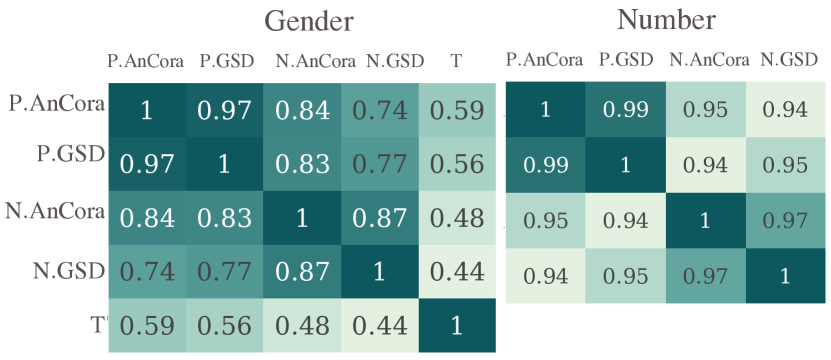
Figure 4: Cosine similarities of the ATE on BERT representations. N. represents $\psi_{\text{na\"{i}ve}}$; P. represents $\psi_{\text{paired}}$; and T. represents $\psi_{\text{paired}}$ estimated on the template-based dataset.

6.1 Variations across ATEs

Variation Across Datasets.

Using our ATE estimators, we compute the average treatment effect of both gender and number on BERT’s contextualized representations (Devlin et al., 2019) of focus nouns. We compute the $\psi_{\text{paired}}$ and $\psi_{\text{na\"{i}ve}}$ estimators. Fig. 4 presents their cosine similarities. We observe high cosine similarities between paired estimators across datasets, but lower cosine similarities with the naïve estimator. This suggests that, while the causal effect is stable across treebanks, the correlational effect is more susceptible to variations in the datasets, e.g., semantic variations due to the domain from which treebanks were sampled.

Templated vs. Naturalistic Counterfactuals.

As an extra baseline, we estimate the ATE using a paired estimator with the template-based dataset introduced in § 5.2 We observe a low cosine similarity between our naturalistic ATE estimates and the template-based ones. This shows that sentences from template-based datasets are substantially different from naturalistic datasets, thus failing to provide unbiased estimates in naturalistic settings.

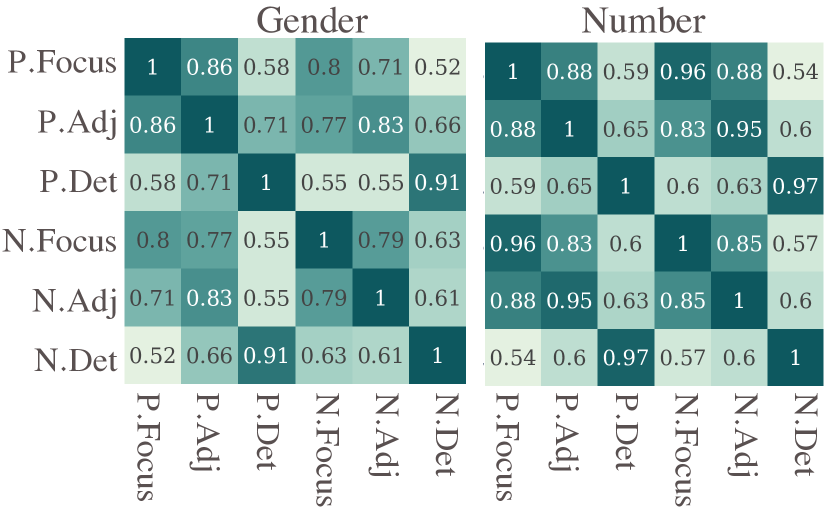
Figure 5: Cosine similarity of ATE estimators computed on focus nouns, adjectives and determiners using BERT representations.

Variation Across Part-of-Speech Tags.

Using the same approach, we additionally compute the ATEs on adjectives and determiners. Fig. 5 presents our naïve and paired ATE estimates, computed on words with different parts of speech. These results suggest that gender and number do not affect the focus noun or its dependent words in the same way. While the ATE on focus nouns and adjectives are strongly aligned, the cosine similarity between ATEs on focus nouns and determiners is smaller.

6.2 Masked Language Modeling Predictions

We now analyze the effect of our morpho-syntactic features on masked language modeling predictions. Specifically, we analyze RoBERTa (Conneau et al., 2020) in these experiments, as it has better performance than BERT in masked prediction. We thus look at how grammatical gender and number affect the probability RoBERTa assigns to each word in its output vocabulary.

		$\mathrm{MProbs}(\mathbf{h})$	$\mathrm{MProbs}(\widehat{\mathbf{h}}_{\psi_{\text{na\"{i}ve}}})$	$\mathrm{MProbs}(\widehat{\mathbf{h}}_{\psi_{\text{paired}}})$
{32.5mm[ gender ]	Det: $\mathrm{MProbs}(\mathbf{h^{\prime}})$	$4.85\pm 2.39$	$1.09\pm 1.4$	$0.67\pm 1.14$
	Adj: $\mathrm{MProbs}(\mathbf{h^{\prime}})$	$2.29\pm 2$	$1.04\pm 1.05$	$0.9\pm 1.12$
	Focus: $\mathrm{MProbs}(\mathbf{h^{\prime}})$	$3.75\pm 2.67$	$1.74\pm 1.11$	$1.53\pm 0.93$
{32.5mm[ number ]	Det: $\mathrm{MProbs}(\mathbf{h^{\prime}})$	$6.93\pm 2.52$	$1.92\pm 2.87$	$2.05\pm 2.64$
	Adj: $\mathrm{MProbs}(\mathbf{h^{\prime}})$	$5.63\pm 2.75$	$2.25\pm 2.2$	$2.5\pm 2.17$
	Focus: $\mathrm{MProbs}(\mathbf{h^{\prime}})$	$5.50\pm 3.02$	$2.25\pm 2.14$	$2.41\pm 1.9$

Table 2: Mean and standard deviation of Jensen–Shannon divergence between the masked probability distributions of focus nouns, determiners and adjectives over the corpus.

We start by masking a word in our sentence: either the focus noun, a dependent determiner, or an adjective. We then obtain this word’s contextual representation $\mathbf{h}$. Second, we apply a syntactic intervention to this sentence, and, following similar steps, obtain another representation $\mathbf{h^{\prime}}$. Third, we use these representations to obtain the probabilities RoBERTa assigns to the words in its vocabulary $\mathrm{MProbs}(\mathbf{h})$ and $\mathrm{MProbs}(\mathbf{h^{\prime}})$. Finally, we get these same probability assignments, but using ATE to estimate the counterfactual representations:

$$\mathrm{MProbs}(\widehat{\mathbf{h}}_{\psi_{\text{paired}}}),\quad \widehat{\mathbf{h}}_{\psi_{\text{paired}}}=\mathbf{h}\pm\psi_{\text{paired}}$$ (11)

$$\mathrm{MProbs}(\widehat{\mathbf{h}}_{\psi_{\text{na\"{i}ve}}}),\quad \widehat{\mathbf{h}}_{\psi_{\text{na\"{i}ve}}}=\mathbf{h}\pm\psi_{\text{na\"{i}ve}}$$ (12)

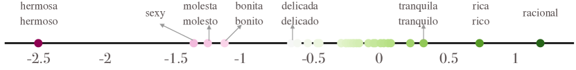
Figure 6: $\psi_{\text{paired}}^{(a)}$ values computed using Eq. 14 to measure causal gender bias in masked adjective prediction.

We now look at how probability assignments change as a function of our interventions. Specifically, Table 2 shows Jensen-–Shannon divergences between $\mathrm{MProbs}(\cdot)$ computed on top of different representations. We can make a number of observations based on this table. First, for gender, these distributions change more when predicting determiners and focus nouns than adjectives. We speculate that this may be because many Spanish adjectives are syncretic, i.e., they have the same inflected form for masculine and feminine, e.g., inteligente (intelligent), or profesional (professional). Second, the distributions change more after an intervention on number than on gender. Third, when we use either of our estimators to approximate the counterfactual representation, the divergences are greatly reduced; These results show that the ATE values do describe (at least to some extent) the change of representations in individual sentences.

6.3 Gender Bias in Adjectives

As shown by Bartl et al. (2020) and Gonen et al. (2022), the results of studies on gender bias in English are not completely transferable to gender-marking languages. We analyze the causal effect of gender on specific masked adjective probabilities, predicted by the RoBERTa model. To this end, we manually create a list of 30 adjectives (the complete list is in App. A) in both masculine and feminine forms. We sample a sentence $\boldsymbol{f}$ from a subset of the dataset in which the focus noun has one dependent adjective $a$, and mask this adjective. We then define a new function $\mathtt{tgt}(\cdot)$ to measure the ATE on adjective probabilities. Specifically, we write:

$$\mathtt{tgt}_{a}(\boldsymbol{f}) =\ln\,p_{\theta}(a\mid\boldsymbol{f})$$ (13)

$$=\ln\,p_{\theta}(a\mid g_{*},\ell_{*},\boldsymbol{z})$$

where $a$ represents an adjective in our list (that also exists in RoBERTa’s vocabulary $\mathcal{V}$) and $p_{\theta}(a\mid\boldsymbol{f})$ is the probability RoBERTa assigns to that adjective. We plug this new function into our paired ATE estimator in Eq. 9. As this prediction is somewhat susceptible to noise, we replace the mean in Eq. 9 with the median, i.e., we compute:

$$\psi_{\text{paired}}^{(a)}=\underset{\langle\_,\ell_{*},\boldsymbol{z}\rangle\in\mathcal{S}}{\mathrm{median}}\left[\ln\,\frac{p_{\theta}(a\mid\textsc{msc},\ell_{*},\boldsymbol{z})}{p_{\theta}(a\mid\textsc{fem},\ell_{*},\boldsymbol{z})}\right]$$ (14)

In this equation, if $\psi_{\text{paired}}^{(a)}>0$, the predicted probability that the adjective appears in a sentence where it is dependent on a masculine focus noun will be typically higher than in a sentence with a feminine focus noun. Whereas if $\psi_{\text{paired}}^{(a)}<0$ the reverse will hold. Therefore, we say $a$ is biased towards masculine gender if $\psi_{\text{paired}}^{(a)}>0$ and it is biased towards feminine gender if $\psi_{\text{paired}}^{(a)}<0$ As shown in Fig. 6, rich (rica/rico) and rational (racional) are more biased towards masculine gender, while beautiful (hermosa/hermoso) is biased towards feminine gender.

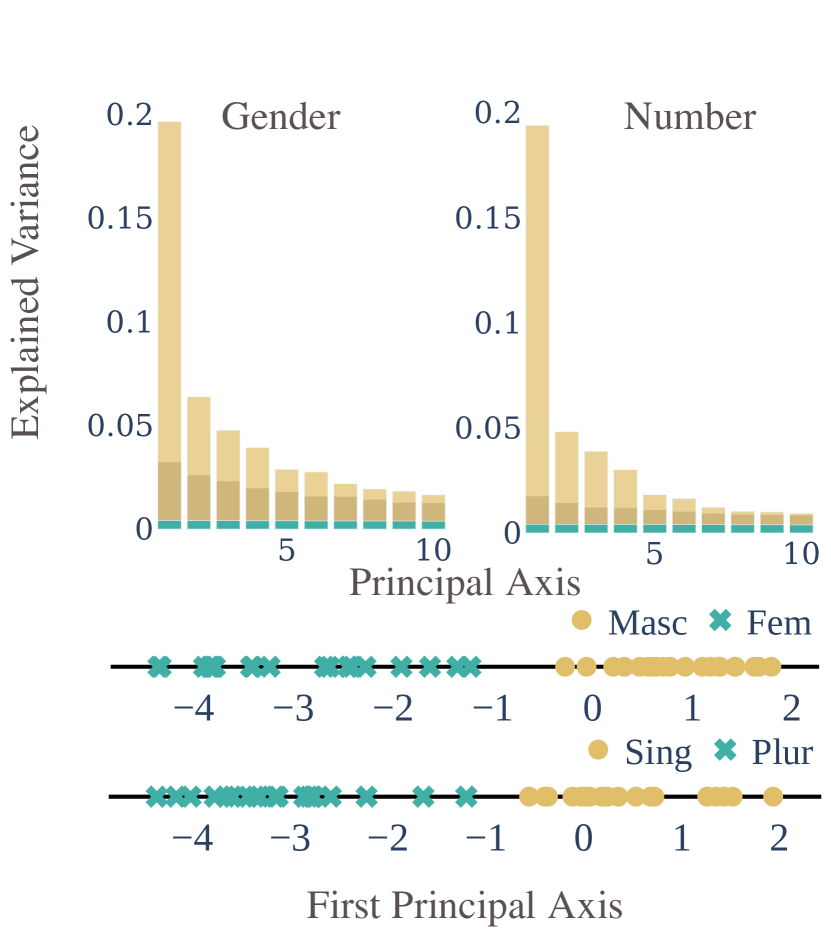
(a) BERT

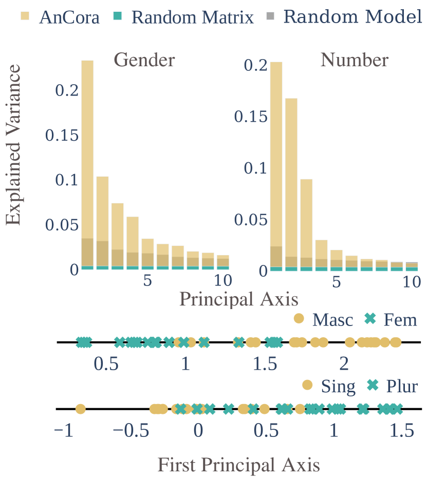
(b) RoBERTa

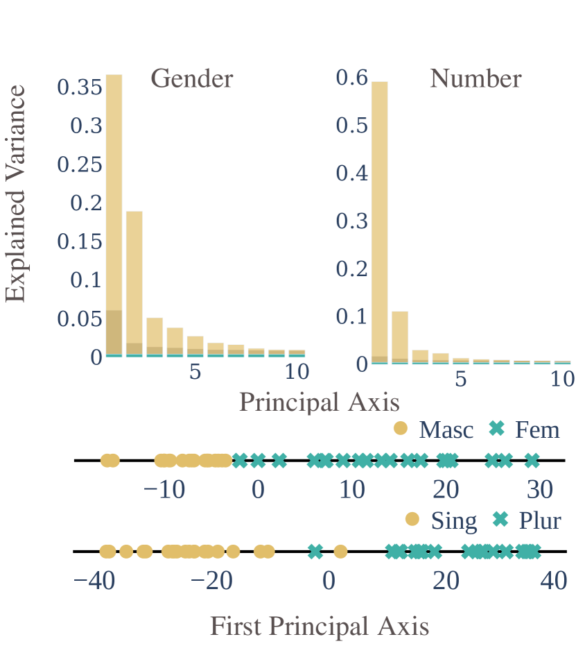
(c) GPT-2

Figure 7: (top) Percentage of the gender and number variance explained by the first 10 PCA components. (bottom) The projection of 20 pairs of focus noun’s representations on the first principal component.

7 Insights From Naturalistic Counterfactuals

In the following experiments, we rely on a dataset augmented with naturalistic counterfactuals. We first explore the geometry of the encoded morpho-syntactic features. We then run a more classic correlational probing experiment, highlighting the importance of a causal framework when analyzing representations.

7.1 Geometry of Morpho-Syntactic Features

In this experiment, we follow Bolukbasi et al.’s (2016) methodology to isolate the subspace capturing our morpho-syntactic features’ information. First, we create a matrix with the representations of all focus nouns in our counterfactually augmented dataset. Second, we pair each noun’s representation with its counterfactual representation (after the intervention). Third, we center the matrix of representations by subtracting each pair’s mean. Finally, we perform principal component analysis on this new matrix.

As Fig. 7 shows, in BERT and RoBERTa, the first principal component explains close to 20% of the variance caused by gender and number. In GPT-2 (Radford et al., 2019), more than half of the variance is captured by the first or the first two principal components. This result is in line with prior work (e.g., Biasion et al., 2020, on Italian word embeddings), and suggests that these morpho-syntactic features are linearly encoded in the representations.

To further explore the gender and number subspaces, we project a random sample of 20 sentences (along with their counterfactuals) onto the first principal component. Fig. 7 (bottom) shows that the three models we probe can (at least to a large extent) differentiate both morpho-syntactic features using a single dimension. Notably, this first principal component is strongly aligned with the estimate $\psi_{\text{paired}}$; they have a cosine similarity of roughly 0.99 in all these settings.

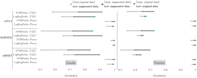
Figure 8: Accuracy scores of gender and number probes on the original and augmented datasets.

7.2 Analysis of Correlational Probing

We now use a dataset augmented with naturalistic counterfactuals to empirically evaluate the entanglement of correlation and causation discussed in § 2, which arises when using diagnostic probes to probe the representations. Again, we probe three contextual representations: BERT, RoBERTa, and GPT-2. We train logistic regressors (LogRegProbe) and support vector machines (SVMProbe) to predict either gender or number of the focus noun from its contextual representation. Further, we probe the representations in two positions: the focus noun and the $\mathtt{[CLS]}$ token (or a sentence’s last token, for GPT-2).

Accuracy of correlational probes on the original dataset is shown in Fig. 8 as green points. Both gender and number probes reach a near-perfect accuracy on focus nouns’ representations. Furthermore, all correlational gender probes reach a high accuracy in $\mathtt{[CLS]}$ representations, suggesting that gender can be reliably recovered from them.

Next, we evaluate trained probes on counterfactually augmented test sets (shown as yellow points in Fig. 8). We see that there is a drop in performance in all settings, and more specifically, the accuracy of probes on $\mathtt{[CLS]}$ representations drops significantly when evaluated on the counterfactual test set. This suggest that the previous results using correlational probes overestimate the extent to which gender and number can be predicted from the representations.

Finally, we also train supervised probes on a counterfactually augmented dataset in order to study whether we can achieve the levels of performance attested in the literature (shown as gray points in Fig. 8). Since these probes are trained on a dataset augmented with counterfactuals, they are not as susceptible to spurious correlations; we thus call them the causal probes. Although there is a considerable improvement in accuracy, there is still a large gap between correlational and causal probes’ accuracies. Together, these results imply that correlational probes are sensitive to spurious correlations in the data (such as the semantic context in which nouns appear), and do not learn to predict grammatical gender robustly.

8 Conclusion

We propose a heuristic algorithm for syntactic intervention which, when applied to naturalistic data, allows us to create naturalistic counterfactuals. Although similar analyses have been run by prior work, using either templated or representational counterfactuals (Elazar et al., 2021; Vig et al., 2020; Bolukbasi et al., 2016, inter alia), our syntactic intervention approach allows us to run these analyses on naturalistic data. We further discuss how to use these counterfactuals in a causal setting to probe for morpho-syntax. Experimentally, we first showed that ATE estimates are more robust to dataset differences than either our naïve (correlational) estimator, or template-based approaches. Second, we showed that ATE can (at least partially) predict how representations will be affected after intervention on gender or number. Third, we employ our ATE framework to study gender bias, finding a list of adjectives that are biased towards one or other gender. Fourth, we find that the variation of gender and number can be captured by a few principal axes in the nouns’ representations. And, finally, we highlight the importance of causal analyses when probing: When evaluated on counterfactually augmented data, correlational probe results drop significantly.

Ethical Concerns

Pretrained models often encode gender bias. The adjective bias experiments in this work can provide further insights into the extent to which these biases are encoded in multilingual pretrained models. As our paper focuses on (grammatical) gender as a morpho-syntactic feature, it focuses on a binary notion of gender, which is not representative of the full spectrum of human gender expression. Most of the analysis in this paper focuses on measuring grammatical gender, not gender bias. We thus advise caution when interpreting the findings from this work. Nonetheless, we hope the causal structure formalized here, together with our analyses, can be of use to bias mitigation techniques in future (e.g., Liang et al., 2020).

Appendix A List of Adjectives

We use 30 different Spanish adjectives in our experiments: hermoso/hermosa (beautiful), sexy (sexy), molest/molesta (upset), bonito/bonita (pretty), delicado/delicada (delicate), rápido/rápida (fast), joven (young), inteligente (intelligent), divertido/divertida (funny), fuerte (strong), duro/dura (hard), alegre (cheerful), protegido/protegida (protected), excelente (excellent), nuevo/nueva (new), serio/seria (serious), sensible (sensitive), profesional (professional), emocional (emotional), independiente (independent), fantástico/fantástica (fantastic), brutal (brutal), malo/mala (bad), bueno/buena (good), horrible (horrible), triste (sad), amable (nice), tranquilo/tranquila (quiet), rico/rica (rich), racional (rational).

Appendix B Algorithm for Heuristic Intervention

1:procedure ReinflectTree($\mathtt{node}$, $\mathtt{parent}$, $\mathtt{state}$)

2:   $\mathtt{isFocusNoun}$$\;\leftarrow\;$ $\mathtt{false}$

3:   if $\mathtt{state}$$==$ $\mathtt{NORMAL}$ and $\mathtt{node}$  is a valid noun :

4:     ReinflectNoun($\mathtt{node}$) $\triangleright$ Change the noun and set the morpho-syntactic feature to the desired value

5:     $\mathtt{isFocusNoun}$$\;\leftarrow\;$ $\mathtt{true}$

6:     if $\mathtt{node}$  is subject :

7:        ReinflectVerb($\mathtt{parent}$) $\triangleright$ Change verb         

8:   if $\mathtt{state}$$==$ $\mathtt{DIR}$  : $\triangleright$ Current node is a direct dependent of a focus noun

9:     if $\mathtt{node}$  is a determiner :

10:        ReinflectDet($\mathtt{node}$) $\triangleright$ Change determiner      

11:     if $\mathtt{node}$  is an adjective modifier :

12:        ReinflectAdj($\mathtt{node}$) $\triangleright$ Change adjective      

13:     if $\mathtt{node}$  is a nominal subject :

14:        ReinflectNoun($\mathtt{node}$) $\triangleright$ Change noun

15:        $\mathtt{nsubj}$$\;\leftarrow\;$ $\mathtt{true}$     

16:     if $\mathtt{node}$  is a copula :

17:        ReinflectCop($\mathtt{node}$) $\triangleright$ Change copula         

18:   if $\mathtt{state}$$==$ $\mathtt{INDIR}$ and $\mathtt{node}$  is an adjective modifier and $\mathtt{parent}$  is an adjective modifier : $\triangleright$ Current node is a descendant of a focus noun

19:     ReinflectAdj($\mathtt{node}$)    

20:   for $\mathtt{child}$ $\in$ children($\mathtt{node}$) :

21:     if $\mathtt{isFocusNoun}$  or $\mathtt{nsubj}$ :

22:        ReinflectTree($\mathtt{child}$, $\mathtt{node}$, $\mathtt{DIR}$ )

23:     else if $\mathtt{state}$$==$ $\mathtt{DIR}$ or $\mathtt{state}$$==$ $\mathtt{INDIR}$  :

24:        ReinflectTree($\mathtt{child}$, $\mathtt{node}$, $\mathtt{INDIR}$ )

25:     else

26:        ReinflectTree($\mathtt{child}$, $\mathtt{node}$, $\mathtt{NORMAL}$ )         

Appendix C Theory

Proposition 1.

In this proposition we show that the average treatment effect is equivalent to the difference of two expectations with no do-operator:

$$\operatorname*{\mathbb{E}}_{\boldsymbol{F}}\Big{[}\mathtt{tgt}(\boldsymbol{F})\mid \,\mathrm{do}\left(G_{*}=\textsc{msc}\right)\Big{]}-\operatorname*{\mathbb{E}}_{\boldsymbol{F}}\Big{[}\mathtt{tgt}(\boldsymbol{F})\mid\mathrm{do}\left(G_{*}=\textsc{fem}\right)\Big{]}$$ (15)

$$=\operatorname*{\mathbb{E}}_{L_{*},\boldsymbol{Z}}\left[\operatorname*{\mathbb{E}}_{\boldsymbol{F}}\Big{[}\mathtt{tgt}(\boldsymbol{F})\mid G_{*}=\textsc{msc},L_{*},\boldsymbol{Z}\Big{]}\right]-\operatorname*{\mathbb{E}}_{L_{*},\boldsymbol{Z}}\left[\operatorname*{\mathbb{E}}_{\boldsymbol{F}}\Big{[}\mathtt{tgt}(\boldsymbol{F})\mid G_{*}=\textsc{fem},L_{*},\boldsymbol{Z}\Big{]}\right]$$

Proof.

First, we note the existence of two backdoor paths in our model Fig. 3: $M_{*}\leftarrow U\rightarrow\boldsymbol{Z}\rightarrow\boldsymbol{F}\rightarrow\mathbf{R}$ and $M_{*}\leftarrow U\rightarrow L_{*}\rightarrow\boldsymbol{F}\rightarrow\mathbf{R}$. We can easily check that $\boldsymbol{Z}$ blocks the first and $L_{*}$ blocks the second path, and neither $\boldsymbol{Z}$ nor $L_{*}$ are descendants of $M_{*}$. Therefore $\{L_{*},\boldsymbol{Z}\}$ satisfies the back-door criterion. To make the proof simpler, we show that the first term of the left-hand side of Eq. 15 equals the first term in the right-hand side of Eq. 15 and then we get the full result by symmetry. We proceed as follows:

$$\operatorname*{\mathbb{E}}_{\boldsymbol{F}}\Big{[}\mathtt{tgt}(\boldsymbol{F})\mid \mathrm{do}\left(G_{*}=\textsc{msc}\right)\Big{]}$$ (16)

$$=\sum_{\ell_{*}\in\mathcal{L}}\sum_{\boldsymbol{z}\in\mathcal{Z}}\operatorname*{\mathbb{E}}_{\boldsymbol{F}}\Big{[}\mathtt{tgt}(\boldsymbol{F})\mid\mathrm{do}(G_{*}=\textsc{msc}),\ell_{*},\boldsymbol{z})\Big{]}p(\ell_{*},\boldsymbol{z})\quad \ell_{*} \boldsymbol{z}$$ (marginalize and )

$$=\sum_{\ell_{*}\in\mathcal{L}}\sum_{\boldsymbol{z}\in\mathcal{Z}}\operatorname*{\mathbb{E}}_{\boldsymbol{F}}\Big{[}\mathtt{tgt}(\boldsymbol{F})\mid G_{*}=\textsc{msc},\ell_{*},\boldsymbol{z})\Big{]}p(\ell_{*},\boldsymbol{z})\quad$$ (backdoor criterion)

$$=\operatorname*{\mathbb{E}}_{L_{*},\boldsymbol{Z}}\left[\operatorname*{\mathbb{E}}_{\boldsymbol{F}}\Big{[}\mathtt{tgt}(\boldsymbol{F})\mid G_{*}=\textsc{msc},L_{*},\boldsymbol{Z}\Big{]}\right]$$ (rewrite as an expectation)

∎

References

- Adi et al. (2017) Yossi Adi, Einat Kermany, Yonatan Belinkov, Ofer Lavi, and Yoav Goldberg. 2017. Fine-grained analysis of sentence embeddings using auxiliary prediction tasks. In 5th International Conference on Learning Representations (Conference Track).
- Alain and Bengio (2017) Guillaume Alain and Yoshua Bengio. 2017. Understanding intermediate layers using linear classifier probes. In 5th International Conference on Learning Representations (Workshop Track).
- Bartl et al. (2020) Marion Bartl, Malvina Nissim, and Albert Gatt. 2020. Unmasking contextual stereotypes: Measuring and mitigating BERT’s gender bias. In Proceedings of the Second Workshop on Gender Bias in Natural Language Processing, pages 1–16, Barcelona, Spain (Online). Association for Computational Linguistics.
- Belinkov (2021) Yonatan Belinkov. 2021. Probing classifiers: Promises, shortcomings, and alternatives. arXiv preprint arXiv:2102.12452.
- Belinkov et al. (2017) Yonatan Belinkov, Lluís Màrquez, Hassan Sajjad, Nadir Durrani, Fahim Dalvi, and James Glass. 2017. Evaluating layers of representation in neural machine translation on part-of-speech and semantic tagging tasks. In Proceedings of the Eighth International Joint Conference on Natural Language Processing (Volume 1: Long Papers), pages 1–10, Taipei, Taiwan. Asian Federation of Natural Language Processing.
- Biasion et al. (2020) Davide Biasion, Alessandro Fabris, Gianmaria Silvello, and Gian Antonio Susto. 2020. Gender bias in italian word embeddings. In Proceedings of the Seventh Italian Conference on Computational Linguistics CLiC-it 2020: Bologna.
- Bolukbasi et al. (2016) Tolga Bolukbasi, Kai-Wei Chang, James Y. Zou, Venkatesh Saligrama, and Adam T. Kalai. 2016. Man is to computer programmer as woman is to homemaker? Debiasing word embeddings. In Advances in Neural Information Processing Systems, volume 29.
- Brown et al. (2001) Lawrence D. Brown, T. Tony Cai, and Anirban DasGupta. 2001. Interval Estimation for a Binomial Proportion. Statistical Science, 16(2):101 – 133.
- Brown et al. (2020) Tom Brown, Benjamin Mann, Nick Ryder, Melanie Subbiah, Jared D Kaplan, Prafulla Dhariwal, Arvind Neelakantan, Pranav Shyam, Girish Sastry, Amanda Askell, Sandhini Agarwal, Ariel Herbert-Voss, Gretchen Krueger, Tom Henighan, Rewon Child, Aditya Ramesh, Daniel Ziegler, Jeffrey Wu, Clemens Winter, Chris Hesse, Mark Chen, Eric Sigler, Mateusz Litwin, Scott Gray, Benjamin Chess, Jack Clark, Christopher Berner, Sam McCandlish, Alec Radford, Ilya Sutskever, and Dario Amodei. 2020. Language models are few-shot learners. In Advances in Neural Information Processing Systems, volume 33, pages 1877–1901.
- Conneau et al. (2020) Alexis Conneau, Kartikay Khandelwal, Naman Goyal, Vishrav Chaudhary, Guillaume Wenzek, Francisco Guzmán, Edouard Grave, Myle Ott, Luke Zettlemoyer, and Veselin Stoyanov. 2020. Unsupervised cross-lingual representation learning at scale. In Proceedings of the 58th Annual Meeting of the Association for Computational Linguistics, pages 8440–8451, Online. Association for Computational Linguistics.
- Conneau et al. (2018) Alexis Conneau, German Kruszewski, Guillaume Lample, Loïc Barrault, and Marco Baroni. 2018. What you can cram into a single $&!#* vector: Probing sentence embeddings for linguistic properties. In Proceedings of the 56th Annual Meeting of the Association for Computational Linguistics (Volume 1: Long Papers), pages 2126–2136, Melbourne, Australia. Association for Computational Linguistics.
- Devlin et al. (2019) Jacob Devlin, Ming-Wei Chang, Kenton Lee, and Kristina Toutanova. 2019. BERT: Pre-training of deep bidirectional transformers for language understanding. In Proceedings of the 2019 Conference of the North American Chapter of the Association for Computational Linguistics: Human Language Technologies, Volume 1 (Long and Short Papers), pages 4171–4186, Minneapolis, Minnesota. Association for Computational Linguistics.
- Elazar et al. (2021) Yanai Elazar, Shauli Ravfogel, Alon Jacovi, and Yoav Goldberg. 2021. Amnesic probing: Behavioral explanation with amnesic counterfactuals. Transactions of the Association for Computational Linguistics.
- Ettinger et al. (2016) Allyson Ettinger, Ahmed Elgohary, and Philip Resnik. 2016. Probing for semantic evidence of composition by means of simple classification tasks. In Proceedings of the 1st Workshop on Evaluating Vector-Space Representations for NLP, pages 134–139, Berlin, Germany. Association for Computational Linguistics.
- Feder et al. (2021) Amir Feder, Nadav Oved, Uri Shalit, and Roi Reichart. 2021. CausaLM: Causal Model Explanation Through Counterfactual Language Models. Computational Linguistics, 47(2):333–386.
- Finlayson et al. (2021) Matthew Finlayson, Aaron Mueller, Sebastian Gehrmann, Stuart Shieber, Tal Linzen, and Yonatan Belinkov. 2021. Causal analysis of syntactic agreement mechanisms in neural language models. In Proceedings of the 59th Annual Meeting of the Association for Computational Linguistics and the 11th International Joint Conference on Natural Language Processing (Volume 1: Long Papers), pages 1828–1843, Online. Association for Computational Linguistics.
- Giulianelli et al. (2018) Mario Giulianelli, Jack Harding, Florian Mohnert, Dieuwke Hupkes, and Willem Zuidema. 2018. Under the hood: Using diagnostic classifiers to investigate and improve how language models track agreement information. In Proceedings of the 2018 EMNLP Workshop BlackboxNLP: Analyzing and Interpreting Neural Networks for NLP, pages 240–248, Brussels, Belgium. Association for Computational Linguistics.
- Gonen et al. (2019) Hila Gonen, Yova Kementchedjhieva, and Yoav Goldberg. 2019. How does grammatical gender affect noun representations in gender-marking languages? In Proceedings of the 23rd Conference on Computational Natural Language Learning (CoNLL), pages 463–471, Hong Kong, China. Association for Computational Linguistics.
- Gonen et al. (2022) Hila Gonen, Shauli Ravfogel, and Yoav Goldberg. 2022. Analyzing gender representation in multilingual models. In Proceedings of the 7th Workshop on Representation Learning for NLP, pages 67–77, Dublin, Ireland. Association for Computational Linguistics.
- Gonzalez-Agirre et al. (2012) Aitor Gonzalez-Agirre, Egoitz Laparra, and German Rigau. 2012. Multilingual central repository version 3.0. In Proceedings of the Eighth International Conference on Language Resources and Evaluation (LREC’12), pages 2525–2529, Istanbul, Turkey. European Language Resources Association (ELRA).
- Hernán and Robins (2020) MA Hernán and JM Robins. 2020. Causal inference: What if. Boca Raton: Chapman & Hall/CRC.
- Hewitt et al. (2021) John Hewitt, Kawin Ethayarajh, Percy Liang, and Christopher Manning. 2021. Conditional probing: Measuring usable information beyond a baseline. In Proceedings of the 2021 Conference on Empirical Methods in Natural Language Processing, pages 1626–1639, Online and Punta Cana, Dominican Republic. Association for Computational Linguistics.
- Hewitt and Liang (2019) John Hewitt and Percy Liang. 2019. Designing and interpreting probes with control tasks. In Proceedings of the 2019 Conference on Empirical Methods in Natural Language Processing and the 9th International Joint Conference on Natural Language Processing (EMNLP-IJCNLP), pages 2733–2743, Hong Kong, China. Association for Computational Linguistics.
- Hupkes et al. (2018) Dieuwke Hupkes, Sara Veldhoen, and Willem Zuidema. 2018. Visualisation and ‘diagnostic classifiers’ reveal how recurrent and recursive neural networks process hierarchical structure. Journal of Artificial Intelligence Research, 61:907–926.
- Joshi et al. (2019) Mandar Joshi, Omer Levy, Luke Zettlemoyer, and Daniel Weld. 2019. BERT for coreference resolution: Baselines and analysis. In Proceedings of the 2019 Conference on Empirical Methods in Natural Language Processing and the 9th International Joint Conference on Natural Language Processing (EMNLP-IJCNLP), pages 5803–5808, Hong Kong, China. Association for Computational Linguistics.
- Kondratyuk (2019) Dan Kondratyuk. 2019. Cross-lingual lemmatization and morphology tagging with two-stage multilingual BERT fine-tuning. In Proceedings of the 16th Workshop on Computational Research in Phonetics, Phonology, and Morphology, pages 12–18, Florence, Italy. Association for Computational Linguistics.
- Lasri et al. (2022) Karim Lasri, Tiago Pimentel, Alessandro Lenci, Thierry Poibeau, and Ryan Cotterell. 2022. Probing for the usage of grammatical number. In Proceedings of the 60th Annual Meeting of the Association for Computational Linguistics (Volume 1: Long Papers), pages 8818–8831, Dublin, Ireland. Association for Computational Linguistics.
- Liang et al. (2020) Paul Pu Liang, Irene Mengze Li, Emily Zheng, Yao Chong Lim, Ruslan Salakhutdinov, and Louis-Philippe Morency. 2020. Towards debiasing sentence representations. In Proceedings of the 58th Annual Meeting of the Association for Computational Linguistics, pages 5502–5515, Online. Association for Computational Linguistics.
- McDonald et al. (2013) Ryan McDonald, Joakim Nivre, Yvonne Quirmbach-Brundage, Yoav Goldberg, Dipanjan Das, Kuzman Ganchev, Keith Hall, Slav Petrov, Hao Zhang, Oscar Täckström, Claudia Bedini, Núria Bertomeu Castelló, and Jungmee Lee. 2013. Universal Dependency annotation for multilingual parsing. In Proceedings of the 51st Annual Meeting of the Association for Computational Linguistics (Volume 2: Short Papers), pages 92–97, Sofia, Bulgaria. Association for Computational Linguistics.
- Nivre et al. (2020) Joakim Nivre, Marie-Catherine de Marneffe, Filip Ginter, Jan Hajič, Christopher D. Manning, Sampo Pyysalo, Sebastian Schuster, Francis Tyers, and Daniel Zeman. 2020. Universal Dependencies v2: An evergrowing multilingual treebank collection. In Proceedings of the 12th Language Resources and Evaluation Conference, pages 4034–4043, Marseille, France. European Language Resources Association.
- Pearl (2009) Judea Pearl. 2009. Causal inference in statistics: An overview. Statistics Surveys, 3:96–146.
- Pimentel and Cotterell (2021) Tiago Pimentel and Ryan Cotterell. 2021. A Bayesian framework for information-theoretic probing. In Proceedings of the 2021 Conference on Empirical Methods in Natural Language Processing, pages 2869–2887, Online and Punta Cana, Dominican Republic. Association for Computational Linguistics.
- Pimentel et al. (2020a) Tiago Pimentel, Naomi Saphra, Adina Williams, and Ryan Cotterell. 2020a. Pareto probing: Trading off accuracy for complexity. In Proceedings of the 2020 Conference on Empirical Methods in Natural Language Processing (EMNLP), pages 3138–3153, Online. Association for Computational Linguistics.
- Pimentel et al. (2020b) Tiago Pimentel, Josef Valvoda, Rowan Hall Maudslay, Ran Zmigrod, Adina Williams, and Ryan Cotterell. 2020b. Information-theoretic probing for linguistic structure. In Proceedings of the 58th Annual Meeting of the Association for Computational Linguistics, pages 4609–4622, Online. Association for Computational Linguistics.
- Radford et al. (2019) Alec Radford, Jeffrey Wu, Rewon Child, David Luan, Dario Amodei, and Ilya Sutskever. 2019. Language models are unsupervised multitask learners. OpenAI blog, 1(8):9.
- Ravfogel et al. (2020) Shauli Ravfogel, Yanai Elazar, Hila Gonen, Michael Twiton, and Yoav Goldberg. 2020. Null it out: Guarding protected attributes by iterative nullspace projection. In Proceedings of the 58th Annual Meeting of the Association for Computational Linguistics, pages 7237–7256, Online. Association for Computational Linguistics.
- Ravfogel et al. (2021) Shauli Ravfogel, Grusha Prasad, Tal Linzen, and Yoav Goldberg. 2021. Counterfactual interventions reveal the causal effect of relative clause representations on agreement prediction. In Proceedings of the 25th Conference on Computational Natural Language Learning, pages 194–209, Online. Association for Computational Linguistics.
- Ravfogel et al. (2022a) Shauli Ravfogel, Michael Twiton, Yoav Goldberg, and Ryan Cotterell. 2022a. Linear relaxed adversarial concept erasure.
- Ravfogel et al. (2022b) Shauli Ravfogel, Francisco Vargas, Yoav Goldberg, and Ryan Cotterell. 2022b. Adversarial concept erasure in kernel space.
- Ravichander et al. (2021) Abhilasha Ravichander, Yonatan Belinkov, and Eduard Hovy. 2021. Probing the probing paradigm: Does probing accuracy entail task relevance? In Proceedings of the 16th Conference of the European Chapter of the Association for Computational Linguistics: Main Volume, pages 3363–3377, Online. Association for Computational Linguistics.
- Rosenbaum and Rubin (1983) Paul R. Rosenbaum and Donald B. Rubin. 1983. The central role of the propensity score in observational studies for causal effects. Biometrika, 70(1):41–55.
- Rudinger et al. (2018) Rachel Rudinger, Jason Naradowsky, Brian Leonard, and Benjamin Van Durme. 2018. Gender bias in coreference resolution. In Proceedings of the 2018 Conference of the North American Chapter of the Association for Computational Linguistics: Human Language Technologies, Volume 2 (Short Papers), pages 8–14, New Orleans, Louisiana. Association for Computational Linguistics.
- Saphra and Lopez (2019) Naomi Saphra and Adam Lopez. 2019. Understanding learning dynamics of language models with SVCCA. In Proceedings of the 2019 Conference of the North American Chapter of the Association for Computational Linguistics: Human Language Technologies, Volume 1 (Long and Short Papers), pages 3257–3267, Minneapolis, Minnesota. Association for Computational Linguistics.
- Stanovsky et al. (2019) Gabriel Stanovsky, Noah A. Smith, and Luke Zettlemoyer. 2019. Evaluating gender bias in machine translation. In Proceedings of the 57th Annual Meeting of the Association for Computational Linguistics, pages 1679–1684, Florence, Italy. Association for Computational Linguistics.
- Taulé et al. (2008) Mariona Taulé, M. Antònia Martí, and Marta Recasens. 2008. AnCora: Multilevel annotated corpora for Catalan and Spanish. In Proceedings of the Sixth International Conference on Language Resources and Evaluation (LREC’08), Marrakech, Morocco. European Language Resources Association (ELRA).
- Tucker et al. (2021) Mycal Tucker, Peng Qian, and Roger Levy. 2021. What if this modified that? syntactic interventions with counterfactual embeddings. In Findings of the Association for Computational Linguistics: ACL-IJCNLP 2021, pages 862–875, Online. Association for Computational Linguistics.
- Vig et al. (2020) Jesse Vig, Sebastian Gehrmann, Yonatan Belinkov, Sharon Qian, Daniel Nevo, Yaron Singer, and Stuart Shieber. 2020. Investigating gender bias in language models using causal mediation analysis. In Advances in Neural Information Processing Systems, volume 33, pages 12388–12401.
- Voita and Titov (2020) Elena Voita and Ivan Titov. 2020. Information-theoretic probing with minimum description length. In Proceedings of the 2020 Conference on Empirical Methods in Natural Language Processing (EMNLP), pages 183–196, Online. Association for Computational Linguistics.
- Wolf et al. (2020) Thomas Wolf, Lysandre Debut, Victor Sanh, Julien Chaumond, Clement Delangue, Anthony Moi, Pierric Cistac, Tim Rault, Rémi Louf, Morgan Funtowicz, Joe Davison, Sam Shleifer, Patrick von Platen, Clara Ma, Yacine Jernite, Julien Plu, Canwen Xu, Teven Le Scao, Sylvain Gugger, Mariama Drame, Quentin Lhoest, and Alexander M. Rush. 2020. Transformers: State-of-the-art natural language processing. In Proceedings of the 2020 Conference on Empirical Methods in Natural Language Processing: System Demonstrations, pages 38–45, Online. Association for Computational Linguistics.
- Zellers et al. (2019) Rowan Zellers, Ari Holtzman, Yonatan Bisk, Ali Farhadi, and Yejin Choi. 2019. HellaSwag: Can a machine really finish your sentence? In Proceedings of the 57th Annual Meeting of the Association for Computational Linguistics, pages 4791–4800, Florence, Italy. Association for Computational Linguistics.
- Zhao et al. (2018) Jieyu Zhao, Tianlu Wang, Mark Yatskar, Vicente Ordonez, and Kai-Wei Chang. 2018. Gender bias in coreference resolution: Evaluation and debiasing methods. In Proceedings of the 2018 Conference of the North American Chapter of the Association for Computational Linguistics: Human Language Technologies, Volume 2 (Short Papers), pages 15–20, New Orleans, Louisiana. Association for Computational Linguistics.
- Zmigrod et al. (2019) Ran Zmigrod, Sabrina J. Mielke, Hanna Wallach, and Ryan Cotterell. 2019. Counterfactual data augmentation for mitigating gender stereotypes in languages with rich morphology. In Proceedings of the 57th Annual Meeting of the Association for Computational Linguistics, pages 1651–1661, Florence, Italy. Association for Computational Linguistics.