The intermediate-ionization lines as virial broadening estimators for Population A quasars

Abstract

The identification of a virial broadening estimator in the quasar UV rest frame suitable for black hole mass computation at high redshift has become an important issue. We compare the HI Balmer H$\beta$  line width to the ones of two intermediate ionization lines: the Aliii$\lambda$1860 doublet and the Ciii]$\lambda$1909 line, over a wide interval of redshift and luminosity ($0\lesssim z\lesssim 3.5$; $43\lesssim\log L\lesssim 48.5$ [erg  s^-1]), for 48 sources belonging to the quasar population characterized by mid-to-high values of the Eddington ratio (Population A). The present analysis indicates that the line width of Aliii$\lambda$1860  and H$\beta$ are highly correlated, and can be considered equivalent for most Population A quasars over five orders of magnitude in luminosity; for Ciii]$\lambda$1909, multiplication by a constant correction factor $\xi\approx 1.25$ is sufficient to bring the FWHM of Ciii] in agreement with the one of H$\beta$. The statistical concordance between low-ionization and intermediate-ionization lines suggests that they predominantly arise from the same virialized part of the broad line region. However, blueshifts of modest amplitude (few hundred km s^-1) with respect to the quasar rest frame and an excess ($\lesssim 1.1$) Aliii broadening with respect to H$\beta$ are found in a fraction of our sample. Scaling laws to estimate $M_{\rm BH}$ of high redshift quasar using the Aliii and the Ciii] line widths have rms scatter $\approx$ 0.3 dex. The Aliii scaling law takes the form $\log M_{\mathrm{BH}}\approx 0.58\log L_{1700,44}+2\log\mathrm{FWHM}+0.49$ [M_⊙].

1 Introduction

The energetics of all accretion-related phenomena occurring in active galactic nuclei (AGN) can be tied down to the mass of the central black hole. The mass ($M_{\rm BH}$) of the black holes at the origin of the AGN phenomenon is now reputed a key parameter in the evolution of galaxies and in cosmology as well (e.g., Kormendy & Ho, 2013; Vogelsberger et al., 2014; Heckman & Best, 2014), and its estimation has become an important branch of extragalactic research. Black hole mass estimates on large type-1 AGN samples are carried out employing a deceptively-simple formulation of the virial theorem, under the assumption that all the mass of the system is concentrated in the center of gravity provided by the black hole (see e.g., Marziani & Sulentic, 2012; Shen, 2013; Peterson, 2014, for reviews): $M_{\rm BH}$= $f_{\mathrm{S}}r_{\mathrm{BLR}}(\delta v)^{2}/G$, where $f_{\mathrm{S}}$ is a structure factor (a.k.a. virial or form factor) dependent on the emitting region geometry and dynamics, the radius $r_{\mathrm{BLR}}$ the distance of the line emitting region from the continuum source, and $\delta v$ a suitable measure of the line broadening (e.g., FWHM or dispersion $\sigma$, Vestergaard & Peterson 2006; Peterson et al. 2004). The main underlying assumptions are that the broadening is due to Doppler effect because of the line emitting gas motion, and that the velocity field is such that the emitting gas remains gravitationally bound to the black hole.

Early UV and optical inter-line shift analysis provided evidence that not all the line emitting gas is bound to the black hole (e.g., Gaskell, 1982; Tytler & Fan, 1992; Brotherton et al., 1994; Marziani et al., 1996; Leighly & Moore, 2004). The scenario emerging from more recent studies is that outflows are ubiquitous in active galactic nuclei. They occur under a wide range of physical conditions, and are detected in almost every band of the electromagnetic spectrum and on a wide range of spatial scales, from a few gravitational radii to tens of kpc (e.g., Capetti et al., 1996; Colbert et al., 1998; Everett, 2007; Carniani et al., 2015; Bischetti et al., 2017; Komossa et al., 2018; Kakkad et al., 2020; Vietri et al., 2020; Laurenti et al., 2021). At high luminosity, massive outflows provide feedback effects to the host galaxy (e.g., Fabian, 2012; King & Pounds, 2015; King & Muldrew, 2016; Barai et al., 2018), and are invoked to account for the $M_{\rm BH}$-bulge velocity dispersion correlation (e.g., Kormendy & Ho, 2013, and references therein). For $z\gtrsim 4$, $M_{\rm BH}$ estimates rely on the Civ$\lambda$1549 high-ionization line, and the highest-$z$ sources appear to be almost always high-accretors (Bañados et al., 2018; Nardini et al., 2019). Two studies pointed out 20 years ago the similarity between X-ray and UV properties of high-$z$ quasars and local quasars accreting at high rates (e.g., Mathur, 2000; Sulentic et al., 2000a). The source of concerns is that high-ionization lines such as Civ$\lambda$1549 are subject to a considerable broadening and blueshifts associated with outflow motions already at low redshift (Coatman et al., 2016; Sulentic et al., 2017; Marinello et al., 2020b, see Marinello et al. 2020a for a detailed study of the prototypical source PHL 1092). Overestimates of the virial broadening by a factor as large as $\approx$5 (Netzer et al., 2007; Sulentic et al., 2007; Mejía-Restrepo et al., 2016; Mejía-Restrepo et al., 2018b) for supermassive black holes at high $z$ may even pose a spurious challenge to concordance cosmology (e.g., Trakhtenbrot et al., 2015) and lead to erroneous inferences on the properties of the seed black holes believed to be fledgling precursors of massive black holes.

This paper is focused on the measurement of the line width of the UV intermediate-ionization lines at $\approx 1900$ Å and on their use for black hole mass measurements for large quasar samples, over a wide interval of luminosity and of redshift. The blend at $\lambda 1900$ Å is due, at least in part, to the Aliii$\lambda$1860 doublet and to the Siiii]$\lambda$1892 and Ciii]$\lambda$1909 lines. Aliii is a resonant doublet (${}^{2}P^{o}_{\frac{3}{2},\frac{1}{2}}\rightarrow^{2}S_{\frac{1}{2}}$) while Siiii] and Ciii] are due to inter-combination transitions (${}^{3}P^{o}_{1}\rightarrow^{1}S_{0}$) with widely different critical densities ($\approx 2\cdot 10^{11}$ cm^-3 and $\approx 3\cdot 10^{9}$ cm^-3, respectively; Zheng 1988; Negrete et al. 2012). The parent ionic species imply ionization potentials $15\lesssim\chi_{\mathrm{i}}\lesssim 30$ eV, intermediate between the ones of low-ionization lines (LILs), and the ones of high-ionization lines (HILs; $\chi_{\mathrm{i}}\gtrsim 40-50$ eV). The intermediate-ionization lines (IILs) at 1900 Å are well-placed to provide a high redshift estimator; they can be observed with optical spectrometers up to $z\sim 4$. Observations can be extended in the NIR (13,500 Å) up to $z\sim 5.7$ without solution of continuity, thereby sampling a redshift domain that is crucial for understanding the primordial growth of massive black holes and galaxy formation. In principle, observations could be extended to the H band to cover the as yet mostly uncharged range $6.5\lesssim z\lesssim 8$, a feat that may well become possible with the advent of James Webb Space Telescope (Gardner et al., 2006), of the ESO Extremely Large Telescope (Gilmozzi & Spyromilio, 2007), and of the next-generation large-aperture telescopes (see e.g., D’Onofrio & Marziani, 2018, for a review of foreseeable technological developments).

The quasar main sequence provides much needed discerning abilities for the exploitation of the IILs (e.g., Sulentic et al., 2000a; Bachev et al., 2004; Marziani et al., 2001; Shen & Ho, 2014; Panda et al., 2018), as line profiles and intensities of individual sources are not considered as isolated entities, but interpreted as part of consolidated trends in the main sequence context. Broad line measurements involving H$\beta$ line width and Feii strength are not randomly distributed but instead define a sequence that has become known as the quasar “main sequence” (MS; e.g., Sulentic et al. 2000a; Shen & Ho 2014; Panda et al. 2019; Wildy et al. 2019). The Feii strength is parameterized by the intensity ratio involving the Feii blue blend at 4570 Å and broad H$\beta$ i.e., $R_{\rm FeII}$= I(Feii$\lambda$4570)/I(H$\beta$), and the Hydrogen H$\beta$ line width by its FWHM. MS sources with higher $R_{\rm FeII}$  show narrower broad H$\beta$  (Population A, FWHM(H$\beta$)$\lesssim 4000$ km s^-1), and sources with broader H$\beta$ profiles tendentially show low $R_{\rm FeII}$  (Pop. B with FWHM(H$\beta$)$\gtrsim 4000$ km s^-1, Sulentic et al. 2000a, 2011). It is also known that optical and UV observational properties are correlated (e.g., Sulentic et al., 2000b; Bachev et al., 2004; Sulentic et al., 2007; Du et al., 2016; Śniegowska et al., 2018). In this paper, the attention is restricted to sources radiating at relatively high Eddington ratio ($L/L_{\rm Edd}$ $\gtrsim 0.1-0.2$) i.e., to Population A that accounts for the large majority of sources discovered at high $z$. In the course of our analysis we realised that sources radiating at lower Eddington ratio ($0.01\ \lesssim$$L/L_{\rm Edd}$ $\lesssim 0.1-0.2$) show a different behaviour of the 1900 blend and will be considered elsewhere.

The coverage of the H$\beta$ spectral range greatly easies the determination of the redshift as well as the positional classification of sources along the MS. In addition, FWHM H$\beta$ has been employed as a virial broadening estimator of $M_{\rm BH}$ since the earliest single-epoch observations of large samples of quasars, and in more recent times as well (e.g., McLure & Jarvis, 2002; McLure & Dunlop, 2004; Vestergaard & Peterson, 2006; Assef et al., 2011; Trakhtenbrot & Netzer, 2012; Shen & Liu, 2012). The H$\beta$ line is likely to be still the most widely used line for $M_{\rm BH}$ computations for low redshift quasars ($z\lesssim 1$). Our analysis relies on the availability of both H$\beta$ and the 1900 blend lines, as we will consider FWHM H$\beta$ as the reference “virial broadening estimator” (VBE).

Section 2 introduces the samples used in the present work, covering a wide range in redshift and luminosity, $0\lesssim z\lesssim 3.5$; $44\lesssim\log L\lesssim 48.5$ [erg  s^-1]. The data were obtained with instruments operating in widely different spectral ranges (UV, optical, IR); as a consequence, S/N ratio values vary widely and the uncertainty assessment requires a dedicated approach (Section 3, and Appendix A). The Section 4 introduces paired fits to H$\beta$ and the 1900 blend (an atlas is provided in Appendix B), along with several line width measures, and the relation between H$\beta$ and Aliii measurements. A scaling law for $M_{\rm BH}$ determination equivalent to the one based on H$\beta$ but based on the IIL broadening is discussed in Section 5.

2 Sample

Low-luminosity 1900 and H$\beta$ data (FOS^⋆ sample)

We considered a Faint Object Spectrograph (FOS) sample from Sulentic et al. (2007, hereafter S07) as a low-$L$ and low-$z$ sample. For the sake of the present paper, we restrict the S07 sample to 28 sources covering the 1900 blend spectral range and with previous measurements for the H$\beta$ profile and $R_{\rm FeII}$ (FOS^⋆ sample). The spectra covering the H$\beta$ spectral range come from Marziani et al. (2003, hereafter M03), as well as from the SDSS (York et al., 2000) and the 6dF (Jones et al. 2004; Table 1 provides information on the provenience of of individual spectra). The FOS high-resolution grisms yielded an inverse resolution $\lambda/\delta\lambda\sim 1000$, equivalent to typical resolution of the data of M03 and of the SDSS. The S/N is above $\gtrsim 20$ for both the optical and UV low-redshift data. The FOS^⋆ sample has a typical bolometric luminosity $\log L\sim 45.6$ [erg  s^-1] and a redshift $z\lesssim 0.5$.

High-luminosity VLT and TNG data for Hamburg-ESO quasars (HE sample)

The sample of high-$L$ quasars includes 10 sources identified in the Hamburg-ESO survey (Wisotzki et al., 2000) in the redshift range $1.4\lesssim z\lesssim 2.6$. All HE quasars satisfy the condition on the bolometric luminosity $\log L\gtrsim 10^{47.5}$ erg  s^-1 and are discussed in detail by Sulentic et al. (2017, hereafter S17), where Civ$\lambda$1549 and H$\beta$ were analyzed. The sample used in this paper is restricted to the 9 Population A sources with VLT/FORS1 spectra and 1 TNG/DOLORES (HE1347-2457) spectrum that cover the 1900 Å blend. The spectral resolutions at FWHM are $\lesssim 300$ km s^-1 and $\lesssim$ 600 km s^-1 for the spectrographs FORS1 and DOLORES, respectively. The resolution of the ISAAC spectra covering H$\beta$  is $\approx$ 300 km s^-1 (Sulentic et al., 2004). Typical S/N values are $\gtrsim 50$.

Additional high-luminosity sources (ISAAC sample)

Additional ISAAC spectra were obtained under programme 083.B-0273(A), for three targets SDSS J005700.18+143737.7 (catalog ), SDSS J132012.33+142037.1 (catalog ), SDSS J161458.33+144836.9 (catalog ). They have been reduced following the same procedures employed for the HE quasars. The data will be presented in a forthcoming paper (Deconto Machado et al., in preparation). Matching rest-frame UV spectra were collected from the SDSS and BOSS (Smee et al., 2013), with a resolving power $R=\lambda$/FWHM $\sim$ 2000.

High-luminosity sources from the WISSH (WISSH sample)

We included near-infrared (NIR) spectroscopic observations of 7 WISSH Population A quasars QSOs (Vietri et al., 2018), obtained with LUCI at the Large Binocular Telescope and in one case with SINFONI at VLT. Basic information on this sample is provided in Table 1 of Vietri et al. (2018). The matching rest-frame UV spectra are from the SDSS. The higher resolution implies a somewhat lower S/N with respect to the ISAAC spectra; we restrict our analysis to the spectra above a minimum S/N $\approx\,15$. Redshifts measured for this paper agree very well with the values reported by Vietri et al. (2018) if the H$\beta$ profile is sharp; they are lower by 300-400 km s^-1 in four cases with relatively shallow profiles due to the different fitting techniques.

Joint sample

Table 1 lists in the following order source identification, redshift, specific rest-frame flux in the UV at 1700 Å $f_{\lambda,1700}$, S/N at 1700 Å  reference to the origin of the spectrum, specific flux in the optical at 5100 Å ($f_{\lambda,5100}$), S/N at 5100 Å, and reference to the origin of the optical spectrum. Table footnotes list references to the flux scale origin, in case the spectrum had uncertain of no absolute spectrophotometric flux calibration. Notes include the radio loudness classification (Zamfir et al., 2008; Ganci et al., 2019): radio-loud (RL), radio-intermediate (RI), and radio-quiet (RQ). Only two sources (HE 0043-2300 (catalog ) and 3C 57 (catalog )) are “jetted” in the sense of having a powerful relativistic jet (Padovani, 2017). HE 0043-2300 (catalog ) is listed as a flat-spectrum radio quasar with dominant blazar characteristics in the Roma-BZCAT (Massaro et al., 2009), and 3C 57 (catalog ) is a compact-steep source (CSS; O’Dea 1998, Sulentic et al. 2015). Two other sources qualify as radio-intermediate (HE 0132-4313 (catalog ) and HE0248-3628 (catalog )), and are briefly discussed in Appendix C.

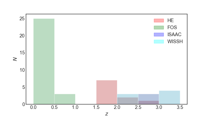
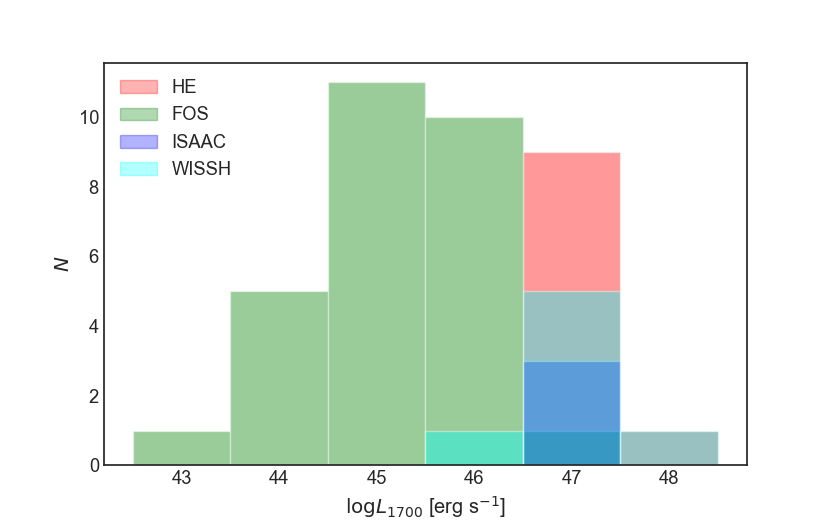
Figure 1: Distribution of redshift (left) and of luminosity at 1700 Å (right) for the four sub-samples considered in this paper.

Table 1: Sample properties

IAU code	Common name	z	$f_{\lambda,1700}$	S/N1700	Ref.	$f_{\lambda,5100}$	S/N5100	Ref.	Notes
FOS⋆ sample
J00063+2012	MRK 0335	0.0252	60.8	15	S07	5.92	55	M03
J00392-5117	[WPV85] 007	0.0290	2.5	15	S07	2.02	45	6dF
J00535+1241	UGC 00545	0.0605	28.2	40	S07	5.77	70	M03
J00573-2222	TON S180	0.0620	31.8	45	S07	14.6	55	M03
J01342-4258	HE 0132-4313	0.2370	15.2	50	S07	1.44	15	6dF	RI
J02019-1132	3C 057	0.6713	17.7	25	S07	1.90	35	S15	CSS
J06300+6905	HS 0624+6907	0.3702	51.7	30	S07	5.04	40	M03
J07086-4933	1H 0707-495	0.0408	22.2	20	S07	2.14	35	6dF
J08535+4349	[HB89] 0850+440	0.5149	5.7	20	S07	0.50	15	M03
J09199+5106	NGC 2841 UB3	0.5563	11.0	30	S07	1.25	40	SDSS
J09568+4115	PG 0953+414	0.2347	17.1	30	S07	2.15	75	M03
J10040+2855	PG 1001+291	0.3298	17.2	25	S07	1.92	45	M03
J10043+0513	PG 1001+054	0.1611	4.9	10	S07	1.50	30	M03
J11185+4025	PG 1115+407	0.1536	11.7	20	S07	0.46	30	M03
J11191+2119	PG 1116+215	0.1765	41.3	40	S07	2.62	50	M03
J12142+1403	PG 1211+143	0.0811	31.0	20	S07	5.45	40	M03
J12217+7518	MRK 0205	0.0711	23.6	35	S07	1.73	55	M03
J13012+5902	SBS 1259+593	0.4776	19.1	25	S07	0.59	50	M03
J13238+6541	PG 1322+659	0.1674	9.5	40	S07	0.71	35	M03
J14052+2555	PG 1402+262	0.1633	22.6	25	S07	1.54	45	M03
J14063+2223	PG 1404+226	0.0973	5.8	15	S07	1.12	60	M03
J14170+4456	PG 1415+451	0.1151	10.2	25	S07	0.86	35	M03
J14297+4747	[HB89] 1427+480	0.2199	7.6	30	S07	0.30	55	M03
J14421+3526	MRK 0478	0.0771	28.2	25	S07	2.04	55	M03
J14467+4035	[HB89] 1444+407	0.2670	18.7	45	S07	1.02	20	M03
J15591+3501	UGC 10120	0.0313	7.3	20	S07	2.29	55	SDSS
J21148+0607	[HB89] 2112+059	0.4608	14.9	25	S07	0.81	50	M03
J22426+2943	UGC 12163	0.0245	10.9	40	S07	0.67	25	M03
HE sample
J00456–2243	HE0043-2300	1.5402	15.5	115	S17	3.2	70	S17	RL
J01242–3744	HE0122-3759	2.2004	21.7	95	S17	2.2	30	S17
J02509–3616	HE0248-3628	1.5355	24.2	200	S17	0.8	50	S17	RI, inv. radio sp.
J04012–3951	HE0359-3959	1.5209	12.1	105	S17	1.8	40	S17
J05092–3232	HE0507-3236	1.5759	11.7	160	S17	2.1	25	S17
J05141-3326	HE0512-3329	1.5862	7.7	40	S17	2.7	25	S17
J11065–1821	HE1104-1805	2.3180	23.9	75	S17	3.0	15	S17
J13506–2512	HE1347-2457	2.5986	48.0	75	S17	3.9	50	S17
J21508–3158	HE2147-3212	1.5432	17.0	150	S17	1.7	20	S17
J23555–3953	HE2352-4010	1.5799	35.5	85	S17	6.3	60	S17
ISAAC sample
J00570+1437	SDSSJ005700.18+143737.7	2.6635	14.0	55	SDSS	2.78	40	D22	normalized at 5000 Å
J13202+1420	SDSSJ132012.33+142037.1	2.5357	8.4	40	SDSS	1.32	25	D22	normalized at 5000 Å
J16149+1448	SDSSJ161458.33+144836.9	2.5703	15.3	50	SDSS	2.54	45	D22	normalized at 5000 Å
WISSH sample
0801+5210	SDSS J080117.79+521034.5	3.2565	29.4	30	SDSS	4.12	20	V18
1157+2724	SDSS J115747.99+272459.6	2.2133	4.2	15	SDSS	2.37	25	V18	HiBAL QSO
1201+0116	SDSS J120144.36+011611.6	3.2476	17.0	30	SDSS	3.31	20	V18
1236+6554	SDSS J123641.45+655442.1	3.4170	22.9	45	SDSS	2.30	25	V18
1421+4633	SDSS J142123.97+463318.0	3.4477	20.9	25	SDSS	3.28	15	V18
1521+5202	SDSS J152156.48+520238.5	2.2189	59.8	80	SDSS	8.40	35	V18
2123–0050	SDSS J212329.46-005052.9	2.2791	32.2	60	SDSS	5.75	45	V18

3 Data analysis

3.1 The quasar main sequence as an interpretative aid

In the following the framework of the quasar MS to make assumptions on line shapes, both in the optical and in the UV spectral ranges. There are several papers that provide a description of the main trends associated with the MS. Fraix-Burnet et al. (2017) reviews the main multifrequency trends. Sulentic et al. (2000a, 2011) review the case for two different quasar Populations: Population A (at low $z$, FWHM H$\beta$  $\lesssim 4000$ km s^-1), and Population B (FWHM H$\beta$  $\gtrsim 4000$ km s^-1). The limit is luminosity-dependent (S17), and reaches FWHM $\gtrsim$ 5500 km s^-1 at high luminosity $\log L\sim 48$). In the optical plane of the MS defined by FWHM H$\beta$ vs $R_{\rm FeII}$  Population A has been subdivided into 4 spectral types (STs) according to Feii prominence: A1, with $R_{\rm FeII}$$\lesssim 0.5$; A2, with $0.5\lesssim$ $R_{\rm FeII}$$\lesssim 1.0$; A3, with $1.0\lesssim$ $R_{\rm FeII}$$\lesssim 1.5$; A4, with $1.5\lesssim$ $R_{\rm FeII}$$\lesssim 2.0$ (Sulentic et al., 2002, see also Shen & Ho 2014 for an analogous approach). The condition $R_{\rm FeII}$ $\gtrsim 1.0$ restricts the MS to the tip of high $R_{\rm FeII}$ values, and encompasses 10% of objects (referred to as extreme Population A). At low-$z$ they are mostly narrow-line Seyfert-1 (NLSy1s) driving the MS correlations (Boroson & Green, 1992; Sulentic et al., 2000a; Du et al., 2016). Sources with $R_{\rm FeII}$$\gtrsim 2$ do exist (Lipari et al., 1993; Graham et al., 1996) but they are exceedingly rare (less than 1%) in optically-selected samples (Marziani et al., 2013a, hereafter M13a). We therefore group all sources with $R_{\rm FeII}$$\gtrsim 1.5$ in A4.

3.2 Multicomponent $\chi^{2}$-minimization

Resolution and S/N of the available spectra are adequate for a multicomponent nonlinear fitting analysis using the IRAF routine specfit (Kriss, 1994), involving an accurate deconvolution of H$\beta$, [Oiii]$\lambda\lambda$4959,5007, Feii, Heii$\lambda$4686  in the optical, and of Aliii, Ciii]  and Siiii] in the UV. A $\chi^{2}$  minimization analysis is necessary in all cases, since the strongest lines are heavily blended together, and the blend involves also features extended over a broad wavelength range, due to Feii (mainly optical, and UV to a lesser extent) and Feiii (UV only).

3.3 H$\beta$ line

The H$\beta$ Balmer emission line is a reliable estimator of the “virial” broadening in samples of moderate-to-high luminosity (Wang et al., 2009; Trakhtenbrot & Netzer, 2012; Shen & Liu, 2012). Typically, the H$\beta$ line profiles are fairly symmetric, and are thought to be dominated by a virialized component (Peterson & Wandel, 1999; Peterson et al., 2004, S17). Several previous works noted that H$\beta$ shows a Lorentzian-like profile in sources belonging to Population A (e.g., Véron-Cetty et al., 2001; Sulentic et al., 2002; Cracco et al., 2016, this is also seen in Mgii$\lambda$2800, Marziani et al. 2013b; Popović et al. 2019). However, the H$\beta$ profiles can be affected by slight asymmetries and small centroid shifts. In Population A they are mostly due to blueshifted excess, often modeled with a blueward asymmetric Gaussian component (BLUE), strongly affecting the Civ$\lambda$1549 line profiles, and related to outflows (e.g., S17, and references therein, Negrete et al. 2018). In H$\beta$, BLUE is detected as a faint excess on the blue side of the symmetric profile assumed as the virialized component of H$\beta$, almost only in extreme Population A (several examples are shown in the Figures of the atlas of Appendix B). Even when the BLUE component is detected, its influence on the H$\beta$ FWHM is modest, leading at most to an increase of the broadening $\approx 10$%  over the FWHM of the symmetric broad profile (Negrete et al., 2018).

To extract a profile that excludes the blueshifted excess, we considered a model of the broad H$\beta$ line with the following components (based on the approach of Negrete et al. 2018):

• the H$\beta_{\rm BC}$, modeled with an (almost) unshifted Lorentzian profile;

• a blueshifted excess (BLUE) modeled with a blueshifted Gaussian with free skew parameter (Azzalini & Regoli, 2012). The skewed Gaussian function has no more outliers than the normal distribution, and retains the shape of the normal distribution on the skewed side. It is consistent with the suppression of the receding side of an optically thin flow obscured by an optically thick structure (i.e., the accretion disk);

• the H$\beta_{\rm NC}$, modeled with a Gaussian, unshifted with respect to rest frame;

• Feii emission, modeled with a scaled and broadened template (e.g., Boroson & Green, 1992), as defined by Negrete et al. (2018);

• [Oiii]$\lambda\lambda$4959,5007, modeled by a core-component (assumed Gaussian and symmetric) and a semi-broad component (assumed Gaussian but with the possibility of being skewed). This approach has been followed in several previous work (e.g., Zhang et al., 2011);

• Heii$\lambda$4686, broad and narrow component. Heii$\lambda$4686 is not always detected in the spectra, especially in the case of strong Feii emission, but the line was included in the fits.

3.4 The 1900 blend

The range 1700 – 2000 is dominated by the 1900Å blend which includes Aliii, Siiii], Ciii], as well as Feii and Feiii lines. On the blue side of the blend Siii$\lambda$1816 and Niii]$\lambda$1750 are also detected. The relative intensity of these lines (apart from Niii]$\lambda$1750 that is not affecting the blend and for which further observations are needed) is known to be a function of the location along the quasar main sequence (Bachev et al., 2004). The line profiles and relative intensities are systematically different not only between Population A and B, but also within Pop. A there is a systematic trend of increasing Aliii and decreasing Ciii] prominence with increasing Feii emission (Bachev et al., 2004).

Our interpretation of the 1900 blend for Population A sources closely follows previous analyses (Baldwin et al., 1996; Wills et al., 1999; Baldwin et al., 2004; Richards et al., 2011; Negrete et al., 2012; Martínez-Aldama et al., 2018). The fits include the following components (described in detail by Martínez-Aldama et al. 2018):

• Aliii, Siiii], and Ciii], modeled with a Lorentzian profile. We assume that the shapes of the strongest lines are consistent with the ones considered for the H$\beta$  broad components (Lorentzian for Pop. A), and that FWHM Aliii = FWHM Siiii] (Negrete et al., 2013). The fitting routine may introduce a systematic blueshift to minimize $\chi^{2}$, in the case the profile is significantly affected by an unresolved blue shifted component, as observed in the case of Mgii$\lambda$2800 ( M13a, );

• Feiii emission, very intense in extreme Population A spectra, modeled with an empirical template (Vestergaard & Wilkes, 2001). Recent photoionization calculations indicate a more significant contribution of Feiii emission in correspondence of Siiii] (Temple et al., 2020). However, the new Feiii model spectrum is consistent with the empirical template of Vestergaard & Wilkes (2001).

  The Feiii template is usually included with the peak shift of Ciii] free to vary in the interval 1908 – 1915 Å (see Martínez-Aldama et al. 2018). In the case the peak shift is around $1914$ Å, the Feiii component may be representing more the $\lambda$1914 line anomalously enhanced by Ly$\alpha$ fluorescence than Ciii]. Considering the severe blending of these two lines, and the weakness of Ciii] in Population A, the relative contribution of Ciii] and Feiii $\lambda$1914 cannot be measured properly. However, if the peak wavelength of the blend around Ciii] is close to 1914 Å, the Feiii $\lambda$1914 line was included in the fit;

• Siii$\lambda$1816, usually fainter than Aliii. This line is expected to be stronger in extreme Population A (Negrete et al., 2012);

• Feii emission, modeled with a scaled and broadened theoretical template (Bruhweiler & Verner, 2008; Martínez-Aldama et al., 2018). The Feii_UV emission is never very strong around 1900 Å, and at any rate gives rise to an almost flat pseudo-continuum that is not affecting the relative intensity ratios of the Aliii, Siiii], Ciii] lines. A spiky feature around 1780 Å is identified with UV Feii multiplet # 191 (Feii$\lambda 1785$). In several extreme cases, attempting to scale the Feii template to the Feii$\lambda 1785$ intensity required large Feii emission (Martínez-Aldama et al., 2018). In such cases the Feii$\lambda 1785$ feature may have been selectively enhanced by Ly$\alpha$ fluorescence over the expectation of the Bruhweiler & Verner (2008) template. Considering the difficult assessment of the Feii_UV emission, no measurements are reported in the present paper.

• a blueshifted excess (BLUE) modeled with a blueshifted skew Gaussian. At high luminosity in the HE sample, there are 2 cases (HE0359-3959 (catalog ) and HE1347-2457 (catalog )) where a strong blueshifted component is obviously affecting the profile of the 1900 blend. Other cases are also detected in the WISSH sample (see §5.3 for the interpretation of the 1900 blend profiles involving a blue shifted excess). For two objects, the BLUE emission is overwhelming and masking the emission of the individual Aliii, Siiii], Ciii] broad components (Section 5.3). Otherwise, the appearance of the blend is not suggesting, even at the highest luminosity, the presence of an outflow component spectroscopically resolved (i.e., of significant blueshifted emission as detected in Civ$\lambda$1549). Small in Aliii blueshifts do occur, but with amplitude $\ll$ than their FWHM.

3.5 Full profile measurements

We assume that the symmetric and unshifted H$\beta_{\rm BC}$  is the representative line components of the virialized part of the BLR. It is expedient to define a parameter $\xi$ as follows:

$$\xi_{\mathrm{line}}={{\rm FWHM}_{\mathrm{vir}}/{\rm FWHM}},$$ (1)

where the FWHM_vir is the FWHM of the “virialized” component, in the following assumed to be H$\beta_{\rm BC}$, and the FWHM is the FWHM measured on the full profile (i.e., without correction for asymmetry and shifts) of any line. In the case of H$\beta$, FWHM H$\beta$ $\approx$ FWHM H$\beta_{\rm BC}$, and $\xi_{\mathrm{H\beta}}\approx 1$ (Section 4.1). For the sake of this work, H$\beta$ and H$\beta_{\rm BC}$ can be considered almost equivalent, so that we will rely on the H$\beta_{\rm BC}$ — H$\beta$ decomposition obtained with specfit only in a few instances. The blue excess is usually faint with respect to H$\beta_{\rm BC}$  and no empirical correction has been applied.

A goal of the present paper is to derive $\xi$ for Aliii and Ciii]. Similarly as for H$\beta$, the Aliii lines are fit by symmetric functions. This approach has been applied in all cases and appears appropriate for the wide majority of spectra ($\approx 90$%), where there is no evidence of a strong BLUE in Aliii and the Aliii peak position is left free to vary to account for small shifts that might be due to a spectroscopically-unresolved outflowing component. A few cases for which there is evidence of contamination by a strong blue shifted excess are discussed in Sect. 5.3.

3.6 Error estimates

The data used in this paper come from an array of instruments yielding spectra with widely different S/N. In addition, the comparison is between two emission lines, one of which is relatively strong ($W$(H$\beta$)$\sim 100$ Å), and one faint ($W$(Aliii)$\lesssim 10$ Å in most cases). To make things worse, at low $z$ the Aliii line is also recorded on lower S/N spectra. These and other systematic differences have to be quantitatively taken into account in the error estimates. A quality parameter $\mathcal{Q}$ has been defined for Aliii, H$\beta$, and Ciii] as the ratio between the line equivalent width and its FWHM multiplied by the S/N ratio measured on the continuum. The $\mathcal{Q}$ values can be computed using the parameters reported in Tables 1 and 2. The systematic differences in the spectra covering Aliii and H$\beta$ are reflected in the distribution of $\mathcal{Q}$: H$\beta$ and Aliii occupy two different domains (Figures in Appendix A). The corresponding fractional uncertainties in FWHM computed from dedicated Markov Chain Monte Carlo (MCMC) simulations or by defining a relation with the $\mathcal{Q}$ parameter as detailed in Appendix A are significantly different for the two lines, being just a few percent in the FWHM of the narrowest sources with strong and sharp H$\beta$ and at worst $\approx 10$%, but in the range $\approx 10$% — 50 % for Aliii.

4 Results

4.1 Immediate results

The specfit analysis results are provided in form of an atlas (Appendix B) for the FOS^⋆, HE, ISAAC, and WISSH samples. The Aliii and H$\beta$ spectral range are shown after continuum subtraction, on a normalized flux scale (at 1700 and 5100 Å). The parameters measured with the specfit analysis or on the full profiles for H$\beta$, and Aliii are reported in Table 2. Table 2 lists, in the following order: identification by IAU code name (Col. 1), rest-frame flux and equivalent width of the H$\beta$ line (Cols. 2–3). The following columns (Cols. 4–6) report the H$\beta$ profile parameters: FWHM H$\beta$, FWHM H$\beta_{\rm BC}$, and shift. Here for shift $s$ we intend the radial velocity of the line peak with respect to the rest frame as defined from the redshift measured in the H$\beta$ spectral range; parameter $R_{\rm FeII}$ and spectral type (Cols. 7–8); rest-frame flux, equivalent width, FWHM and shift of the Aliii line (Cols. 9–12). The FWHM refers to the individual component of the doublet, whereas flux and equivalent width $W$ are measured over the full doublet; flux of Siiii] (Col. 13); Ciii] flux and FWHM (Cols. 14–15). The Feiii flux measurement (Col. 16) was obtained by integrating the template over the range 1800 $-$ 2150 Å. The upper limit of the wavelength range set at 2150 Å allows the inclusion of a broad feature peaking at $\approx 2050-2080$ Å and mostly ascribed to Feiii emission (Martínez-Aldama et al., 2018). Further information on the reported parameters are given in the Table footnotes. Errors on line widths have been computed from the numerical simulations described in Appendix A or from the data listed in Tables 1 and 2 that yield $\mathcal{Q}$. The same approach has been followed for errors on line intensities and line shifts.

The values of the H$\beta$ FWHM for the WISSH quasars are fully consistent with those reported by Vietri et al. (2018) for all but two targets, namely SDSS J152156.48+520238.5 (catalog ) and SDSS J115747.99+272459.6 (catalog ), for which a discrepancy can be explained in terms of a different fitting technique. Intensity ratios computed between lines in the UV and the optical should be viewed with extreme care. The observations are not synoptical and were not collected with the aim of photometric accuracy.

4.2 FWHM H$\beta$ vs. FWHM Aliii

Fig. 2 shows the FWHM Aliii vs FWHM H$\beta$ full profile. The overall consistency in the FWHM of the two lines is rather obvious from the plot. In the case of Aliii and H$\beta$, the Pearson’s correlation coefficient is $\approx 0.785$ ($P\sim 5\cdot 10^{-8}$ of a chance correlation). A best fit with the ordinary least-squares (OLS) bisector yields

$$\mathrm{FWHM\,{AlIII}}\approx(273\pm 216)+(0.933\pm 0.059)\mathrm{FWHM\,H}\beta.$$ (2)

The two lines are, on average, unbiased estimators of each other, with a 0 point offset that reflects the tendency of the Aliii lines to be somewhat broader than H$\beta$ but is not statistically significant (the offset by 250 km s^-1 is at less than 1 $\sigma$ confidence level). An orthogonal LSQ fit yields slope and offset consistent with the OLS. The normalized $\chi_{\nu}^{2}\approx 1$ also indicates that the ratio between the FWHM of the two lines is 1 within the uncertainties. The maximum FWHM $\approx 6000$ km s^-1 is observed for the sources of the highest luminosity (Section 4.4) and is below the luminosity-dependent FWHM limit of Population A.

Fig. 2 should be compared to Fig. 3 of Marziani et al. (2019, hereafter M19), where one can see that there is no obvious relation between the FWHM of Civ$\lambda$1549 and the FWHM of H$\beta$. For the Pop. A sources Civ$\lambda$1549 is systematically broader than H$\beta$, apart from in two cases in the HE sample, and FWHM(Civ$\lambda$1549) shows a broad range of values for similar FWHM H$\beta$ i.e., FWHM(Civ$\lambda$1549) is almost degenerate with respect to H$\beta$. The Civ$\lambda$1549 line FWHM values are so much larger than the ones of H$\beta$  making it possible that the $M_{\rm BH}$ derived from FWHM Civ$\lambda$1549 might be higher by even more than one order of magnitude than the one derived from the H$\beta$ FWHM, as pointed out in several past works (Sulentic et al., 2007; Netzer et al., 2007; Marziani & Sulentic, 2012; Mejía-Restrepo et al., 2016). We remark again that the Aliii line may show a blueshifted excess in 6 sources in our sample, with convincing evidence in only two cases (Sect. 5.3) but that the line profile is otherwise well represented by a symmetric Lorentzian. In the case of a blueshifted excess, the good agreement between FWHM Aliii and FWHM H$\beta$ is in part due to the Siii$\lambda$1816 emission that, if no blueshifted Aliii emission is allowed, becomes very strong in the fit of the 6 sources, and compensate for the blueshifted excess. Siii$\lambda$1816 is expected to be enhanced in the physical conditions of extreme sources (Negrete et al., 2012, Section 5.3). At the same time, including the Siii$\lambda$1816 line in the fits allows for a standard procedure that does not require identification and a screening for the sources with a strong blueshifted excess, which apparently follow the correlation between Aliii and H$\beta$ full profile in Fig. 3.

4.3 Dependence on spectral type and $R_{\rm FeII}$

4.3.1 FWHM

In Fig. 2 the data points are color coded according to their original subsamples. Fig. 3 shows the joint sample FWHM Aliii vs FWHM H$\beta$ full profile color-coded according to ST. There are systematic differences between the various STs, in the sense that A1 sources have Aliii narrower than H$\beta$ (at the relatively high confidence level of 2$\sigma$), and Aliii and H$\beta$ FWHM are almost equal for ST A2. The Aliii and H$\beta$ FWHM ratio is reversed, in the sense that H$\beta$ is narrower than Aliii, for STs A3 and A4 grouped together. The difference between STs is reinforced if only the BC of H$\beta$ is considered (Fig. 4), since the FWHM H$\beta_{\rm BC}$ is slightly lower than the FWHM H$\beta$ of the full H$\beta$ broad profile, with $\xi_{\mathrm{H\beta}}\approx 0.97\pm 0.05$ on average, but $\xi_{\mathrm{H\beta}}\approx 0.79$ for the spectral types A3 and A4. If we define $\xi_{\mathrm{AlIII}}$ = FWHM(H$\beta_{\rm BC}$)/FWHM(Aliii), we have the following median values ($\pm$ semi-interquartile range):

ST	$\mu_{\frac{1}{2}}(1/\xi_{\mathrm{AlIII}})\pm$ SIQR
A3-A4	1.267 $\pm$ 0.223
A2	1.093 $\pm$ 0.176
A1	0.796 $\pm$ 0.158

A2 is the highest-prevalence ST in Population A, with $\xi\approx 1$. However, across Population A there is a significant trend that implies differences of $\pm 20-25$% with respect to unity. The A3-A4 result is after all not surprising, considering that quasars belonging to these spectral types with the strongest Feii emission are the sources most affected by the high-ionization outflows detected in the Civ$\lambda$1549 line. The A1 result i.e., Aliii lines narrower than H$\beta$ by $\approx 20$% comes more as a surprise, and it is intriguing that it is consistent that also for the B Population Aliii is narrower than H$\beta$ (del Olmo et al., in preparation; Marziani et al. 2017). This result may hint at a small but systematic extra broadening not associated with virial motions in A2.

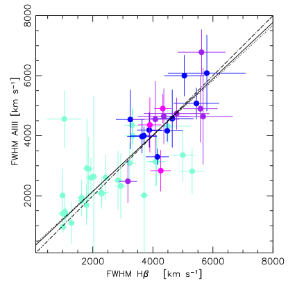
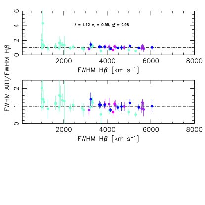
Figure 2: Top panel: FWHM(Aliii) vs. FWHM(H$\beta$) (full profiles) for the joint sample. Data points are color-coded according to sub-sample: FOS^⋆ - aquamarine ($\bullet$), HE - blue ($\bullet$), ISAAC - magenta ($\bullet$), WISSH - purple ($\bullet$). Dot-dashed line: 1:1 relation; filled line: best fit obtained using the bisector technique; dotted line: best fit using the least orthogonal distance method (Press et al., 1992). Middle panel: ratio $r$ of FWHM Aliii over FWHM H$\beta$. The average ratio $\bar{r}$, the standard deviation $\sigma_{\mathrm{r}}$ and the normalized $\chi^{2}_{\nu}$  are reported. Bottom: same as the middle panel, with an expanded scale along the $y$ axis.

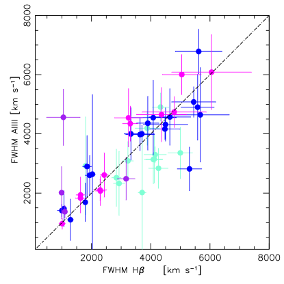
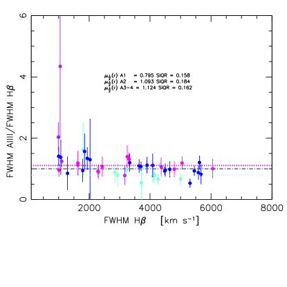
Figure 3: Top panel: FWHM(Aliii) vs. FWHM(H$\beta$) (full profiles) for the joint sample. Data points are color-coded according to spectral type: A1 - aquamarine ($\bullet$), A2 - blue ($\bullet$), A3 - magenta ($\bullet$), A4 - purple ($\bullet$). Bottom: FWHM ratio between Aliii and H$\beta$. The median ratio $\mu_{\frac{1}{2}}(r)$=FWHM Aliii/FWHM H$\beta$, and SIQR are reported for spectral types A1 and A2, and the union of A3 and A4.

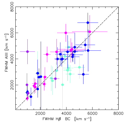
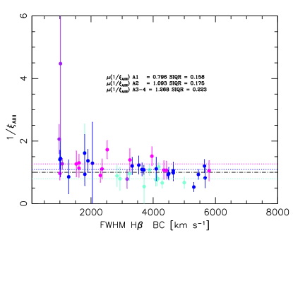
Figure 4: Top panel: FWHM(Aliii) vs. FWHM(H$\beta_{\rm BC}$) for the joint sample. Data points are color-coded according to spectral type as in Fig. 3. Bottom panel: FWHM ratio between Aliii and H$\beta_{\rm BC}$, $1/\xi_{\mathrm{AlIII}}$. The median ratio $\mu_{\frac{1}{2}}(1/\xi_{\mathrm{AlIII}})$ and the SIQR are reported for spectral types A1 and A2, and for the union of A3 and A4, as in Fig. 3.

Table 2: Observed spectrophotometric quantities and main sequence classification

IAU code	H$\beta$					$R_{\rm FeII}$	SpT	Aliii				Siiii]	Ciii]			Feiii
	F	W	FWHM	FWHM BC	Shift			F	W	FWHM	Shift	F	F	FWHM
(1)	(2)	(3)	(4)	(5)	(6)	(7)	(8)	(9)	(10)	(11)	(12)	(13)	(14)	(15)		(16)
FOS sample
J00063+2012	544 $\pm$ 14	99	1790 $\pm$ 82	1802	-130 $\pm$20	0.527 $\pm$ 0.07	A2	92.5 $\pm$ 36.2	1.7	1691 $\pm$ 650	110 $\pm$ 200	316.8 $\pm$ 50.6	345.0 $\pm$ 29.0	800 $\pm$ 77		1579.8 $\pm$ 328.9
J00392-5117	103 $\pm$ 6	50	1290 $\pm$ 100	1283	-10 $\pm$ 20	0.842 $\pm$ 0.09	A2	8.9 $\pm$ 3.0	4.6	1100 $\pm$ 693	-90 $\pm$ 230	21.3 $\pm$ 5.1	50.9 $\pm$ 7.2	1634 $\pm$ 268		90.1 $\pm$ 12.3
J00535+1241	294 $\pm$ 12	45	1100 $\pm$ 64	1077	-30 $\pm$ 20	1.619 $\pm$ 0.06	A4	184.4 $\pm$ 17.2	7.2	1370 $\pm$ 212	-300 $\pm$ 160	321.5 $\pm$ 32.5	277.7 $\pm$ 102.3	1225 $\pm$ 324		857.8 $\pm$ 148.8
J00573-2222	741 $\pm$ 23	47	1070 $\pm$ 30	1019	0 $\pm$ 10	0.737 $\pm$ 0.06	A2	50.2 $\pm$ 9.0	1.6	1473 $\pm$ 602	-270 $\pm$ 240	125.8 $\pm$ 21.3	289.7 $\pm$ 46.3	1672 $\pm$ 224		184.9 $\pm$ 27.3
J01342-4258	35 $\pm$ 5	25	1050 $\pm$ 565	1019	40 $\pm$ 130	2.054 $\pm$ 0.25	A4	71.7 $\pm$ 16.6	5.2	4560 $\pm$ 945	-520 $\pm$ 570	48.6 $\pm$ 22.8	11.7 $\pm$ 3.0	5456 $\pm$ 959		250.6 $\pm$ 35.9
J02019-1132	122 $\pm$ 14	66	4500 $\pm$ 751	4500	30 $\pm$ 140	0.947 $\pm$ 0.15	A2	41.5 $\pm$ 5.5	2.4	4318 $\pm$ 558	250 $\pm$ 450	110.4 $\pm$ 40.5	173.3 $\pm$ 28.3	4318 $\pm$ 965		25.3 $\pm$ 4.6
J06300+6905	167 $\pm$ 6	140	5000 $\pm$ 410	4998	90 $\pm$ 80	0.281 $\pm$ 0.11	A1	137.1 $\pm$ 32.4	2.9	3358 $\pm$ 869	-480 $\pm$ 620	261.6 $\pm$ 126.6	1119.4 $\pm$ 182.0	2962 $\pm$ 504		225.0 $\pm$ 37.5
J07086-4933	74 $\pm$ 5	33	990 $\pm$ 86	980	40 $\pm$ 30	1.717 $\pm$ 0.11	A4	48.9 $\pm$ 17.3	2.2	2015 $\pm$ 874	-140 $\pm$ 620	120.0 $\pm$ 43.6	39.4 $\pm$ 10.4	2188 $\pm$ 432		429.1 $\pm$ 50.6
J08535+4349	73 $\pm$ 6	125	4090 $\pm$ 304	4080	230 $\pm$ 80	0.277 $\pm$ 0.13	A1	18.3 $\pm$ 3.6	3.5	3135 $\pm$ 816	500 $\pm$ 260	50.4 $\pm$ 18.5	59.2 $\pm$ 13.7	1889 $\pm$ 342		63.4 $\pm$ 12.7
J09199+5106	162 $\pm$ 9	106	5310 $\pm$ 411	5310	270 $\pm$ 80	0.878 $\pm$ 0.08	A2	23.6 $\pm$ 6.2	2.2	2817 $\pm$ 733	200 $\pm$ 630	55.3 $\pm$ 12.9	103.3 $\pm$ 26.7	3626 $\pm$ 507		135.4 $\pm$ 39.1
J09568+4115	393 $\pm$ 6	154	3710 $\pm$ 129	3710	180 $\pm$ 30	0.185 $\pm$ 0.08	A1	30.6 $\pm$ 10.7	1.9	2019 $\pm$ 2111	160 $\pm$ 430	50.1 $\pm$ 19.8	188.8 $\pm$ 31.2	1922 $\pm$ 354		157.2 $\pm$ 23.8
J10040+2855	135 $\pm$ 7	63	1940 $\pm$ 151	1900	-40 $\pm$ 40	0.953 $\pm$ 0.09	A2	84.3 $\pm$ 26.9	5.7	2602 $\pm$ 666	-70 $\pm$ 430	141.7 $\pm$ 32.2	140.7 $\pm$ 37.2	1943 $\pm$ 361		101.0 $\pm$ 16.6
J10043+0513	136 $\pm$ 7	90	1850 $\pm$ 143	1800	-110$\pm$ 40	0.694 $\pm$ 0.08	A2	25.6 $\pm$ 9.6	6.2	2898 $\pm$ 1041	-60 $\pm$ 480	72.7 $\pm$ 19.3	73.7 $\pm$ 21.6	1828 $\pm$ 344		117.0 $\pm$ 20.5
J11185+4025	39 $\pm$ 1	83	2030 $\pm$ 95	2050	50 $\pm$ 20	0.588 $\pm$ 0.07	A2	36.7 $\pm$ 12.0	3.5	2638 $\pm$ 2688	230 $\pm$ 390	55.7 $\pm$ 21.8	95.5 $\pm$ 22.4	1963 $\pm$ 464		190.9 $\pm$ 24.6
J11191+2119	406 $\pm$ 17	147	3230 $\pm$ 179	3230	40 $\pm$ 20	0.439 $\pm$ 0.07	A1	180.9 $\pm$ 50.0	5.3	3089 $\pm$ 651	120 $\pm$ 390	413.7 $\pm$ 73.8	510.3 $\pm$ 92.2	2450 $\pm$ 437		883.6 $\pm$ 138.3
J12142+1403	644 $\pm$ 25	111	1800 $\pm$ 92	1800	80 $\pm$ 20	0.424 $\pm$ 0.06	A1	80.9 $\pm$ 34.7	2.9	2922 $\pm$ 1649	-160 $\pm$ 530	117.4 $\pm$ 39.1	349.3 $\pm$ 72.9	1609 $\pm$ 291		420.3 $\pm$ 77.8
J12217+7518	224 $\pm$ 11	135	4120 $\pm$ 280	4120	300 $\pm$ 30	0.255 $\pm$ 0.07	A1	69.1 $\pm$ 22.0	3.2	3149 $\pm$ 804	-310 $\pm$ 430	217.9 $\pm$ 45.6	226.4 $\pm$ 58.5	2246 $\pm$ 416		178.7 $\pm$ 29.4
J13012+5902	37 $\pm$ 2	57	3310 $\pm$ 257	2520	130 $\pm$ 60	1.365 $\pm$ 0.09	A3	136.0 $\pm$ 25.0	8.8	4347 $\pm$ 590	-160 $\pm$ 630	141.8 $\pm$ 42.1	74.0 $\pm$ 30.9	5215 $\pm$ 519		487.2 $\pm$ 95.7
J13238+6541	69 $\pm$ 4	94	2930 $\pm$ 182	2930	-80 $\pm$ 80	0.497 $\pm$ 0.07	A1	12.7 $\pm$ 6.9	1.4	2326 $\pm$ 1075	-320 $\pm$ 770	57.3 $\pm$ 19.0	160.5 $\pm$ 30.0	2076 $\pm$ 399		42.2 $\pm$ 6.9
J14052+2555	73 $\pm$ 4	91	2300 $\pm$ 158	2300	-90 $\pm$ 30	1.15 $\pm$ 0.08	A3	93.3 $\pm$ 28.3	4.8	2073 $\pm$ 491	480 $\pm$ 410	184.2 $\pm$ 38.2	42.7 $\pm$ 14.7	801 $\pm$ 155		559.7 $\pm$ 90.4
J14063+2223	70 $\pm$ 6	59	1630 $\pm$ 151	1530	-10 $\pm$ 30	1.1 $\pm$ 0.11	A3	33.1 $\pm$ 5.1	6.8	1937 $\pm$ 604	-180 $\pm$ 410	62.2 $\pm$ 12.1	31.2 $\pm$ 14.6	1703 $\pm$ 496		121.8 $\pm$ 26.8
J14170+4456	51 $\pm$ 6	63	2290 $\pm$ 217	1620	0 $\pm$ 70	1.182 $\pm$ 0.13	A3	57.6 $\pm$ 4.1	6.4	2104 $\pm$ 353	-80 $\pm$ 250	119.4 $\pm$ 20.4	121.7 $\pm$ 22.5	2010 $\pm$ 234		161.2 $\pm$ 22.0
J14297+4747	48 $\pm$ 2	151	2840 $\pm$ 153	2840	300 $\pm$ 30	0.392 $\pm$ 0.05	A1	14.7 $\pm$ 5.7	2.1	2519 $\pm$ 965	280 $\pm$ 490	29.5 $\pm$ 8.3	92.4 $\pm$ 19.5	1795 $\pm$ 325		79.2 $\pm$ 14.0
J14421+3526	114 $\pm$ 7	55	1630 $\pm$ 169	1610	-140$\pm$ 20	1.357 $\pm$ 0.09	A3	105.8 $\pm$ 32.1	4.0	1832 $\pm$ 433	-260 $\pm$ 410	229.5 $\pm$ 46.9	448.2 $\pm$ 101.3	2007 $\pm$ 366		559.7 $\pm$ 90.4
J14467+4035	77 $\pm$ 3	74	2430 $\pm$ 131	2360	30 $\pm$ 30	1.327 $\pm$ 0.06	A3	62.4 $\pm$ 6.6	3.6	2611 $\pm$ 745	120 $\pm$ 360	142.6 $\pm$ 33.3	106.5 $\pm$ 27.7	2059 $\pm$ 435		373.6 $\pm$ 51.4
J15591+3501	121 $\pm$ 7	44	1010 $\pm$ 105	1000	100 $\pm$ 20	1.424 $\pm$ 0.10	A3	21.1 $\pm$ 2.7	3.3	967 $\pm$ 185	180 $\pm$ 340	64.3 $\pm$ 8.5	152.4 $\pm$ 20.2	1534 $\pm$ 239		150.4 $\pm$ 17.9
J21148+0607	86 $\pm$ 4	119	3330 $\pm$ 228	3320	0 $\pm$ 30	0.781 $\pm$ 0.08	A2	119.0 $\pm$ 34.2	9.3	3999 $\pm$ 883	10 $\pm$ 400	295.2 $\pm$ 55.0	297.1 $\pm$ 54.4	2995 $\pm$ 535		131.9 $\pm$ 20.9
J22426+2943	29 $\pm$ 2	47	1000 $\pm$ 149	1000	-20 $\pm$ 40	0.821 $\pm$ 0.15	A2	18.2 $\pm$ 2.5	1.7	1410 $\pm$ 207	-290 $\pm$ 370	52.3 $\pm$ 4.8	108.1 $\pm$ 28.9	1507 $\pm$ 344		75.2 $\pm$ 10.3
HE sample
J00456–2243	229 $\pm$ 9	68	4150 $\pm$ 370	4146	190 $\pm$ 60	0.37 $\pm$ 0.10	A1	54.0 $\pm$ 4.7	4.1	3299 $\pm$ 261	10 $\pm$ 190	93.0 $\pm$ 16.0	230.0 $\pm$ 63.7	3295 $\pm$ 474		82.0 $\pm$ 15.1
J01242–3744	111 $\pm$ 10	48	3250 $\pm$ 469	3250	0 $\pm$ 100	1.155 $\pm$ 0.14	A3	102.0 $\pm$ 28.8	5.3	4543 $\pm$ 981	10 $\pm$ 390	94.0 $\pm$ 20.5	0.0	…		146.0 $\pm$ 23.0
J02509–3616	39 $\pm$ 3	44	4480 $\pm$ 504	4480	-20 $\pm$ 120	0.531 $\pm$ 0.13	A2	69.0 $\pm$ 4.9	3.1	4164 $\pm$ 345	20 $\pm$ 130	122.0 $\pm$ 13.8	18.0 $\pm$ 2.3	3990 $\pm$ 537		0.0
J04012-3951	88 $\pm$ 9	50	5049 $\pm$ 652	3957	-20 $\pm$ 80	1.103 $\pm$ 0.14	A3	70.0 $\pm$ 8.6	6.2	6003 $\pm$ 673	-150 $\pm$380	39.0 $\pm$ 9.9	17.0 $\pm$ 8.8	2052 $\pm$ 356		122.0 $\pm$ 16.9
J05092–3232	149 $\pm$ 8	67	3880 $\pm$ 403	3880	-130$\pm$ 80	0.311 $\pm$ 0.10	A1	48.0 $\pm$ 6.8	4.3	4193 $\pm$ 574	-50 $\pm$ 450	96.0 $\pm$ 32.3	56.0 $\pm$ 15.4	2500 $\pm$ 467		34.0 $\pm$ 6.2
J05141-3326	228 $\pm$ 15	82	3702 $\pm$ 415	3700	0 $\pm$ 80	0.656 $\pm$ 0.07	A2	57.0 $\pm$ 5.6	7.5	3998 $\pm$ 291	20 $\pm$ 550	129.0 $\pm$ 39.0	67.0 $\pm$ 17.2	2255 $\pm$ 435		81.0 $\pm$ 15.4
J11065–1821	366 $\pm$ 35	121	4647 $\pm$ 702	4646	-50 $\pm$ 110	0.557 $\pm$ 0.11	A2	108.0 $\pm$ 29.6	4.9	4570 $\pm$ 951	0 $\pm$ 390	205.0 $\pm$ 37.1	113.0 $\pm$ 30.8	3138 $\pm$ 576		95.0 $\pm$ 14.8
J13506–2512	162 $\pm$ 29	37	6087 $\pm$ 1346	5795	0 $\pm$ 180	1.266 $\pm$ 0.23	A3	404.0 $\pm$ 101.9	9.5	6087 $\pm$ 1259	-1480 $\pm$620	269.0 $\pm$ 52.5	17.0 $\pm$ 9.6	2190 $\pm$ 652		543.0 $\pm$ 67.0
J21508–3158	120 $\pm$ 9	66	5452 $\pm$ 741	5450	0 $\pm$ 130	0.816 $\pm$ 0.10	A2	104.0 $\pm$ 13.1	7.0	5078 $\pm$ 513	-360 $\pm$190	139.0 $\pm$ 43.3	66.0 $\pm$ 19.0	4095 $\pm$ 696		75.0 $\pm$ 10.2
J23555–3953	318 $\pm$ 21	46	3639 $\pm$ 481	3640	0 $\pm$ 100	0.549 $\pm$ 0.08	A2	99.0 $\pm$ 8.9	3.2	3979 $\pm$ 547	0 $\pm$ 270	150.0 $\pm$ 27.0	0.0	…		370.0 $\pm$ 70.2
ISAAC sample
J00570+1437	219 $\pm$ 15	86.3	3901 $\pm$ 377	3535	-20 $\pm$ 70	0.838 $\pm$ 0.10	A2	120.0 $\pm$ 32.7	10.2	4360 $\pm$ 904	-510 $\pm$ 380	99.0 $\pm$ 21.2	56.0 $\pm$ 16.7	3370 $\pm$ 637		57.9 $\pm$ 9.0
J13202+1420	122 $\pm$ 7	97.0	4262 $\pm$ 325	4290	-150 $\pm$ 80	0.282 $\pm$ 0.05	A1	45.0 $\pm$ 5.3	6.5	2838 $\pm$ 674	-710 $\pm$ 280	78.0 $\pm$ 23.9	96.0 $\pm$ 25.5	3282 $\pm$ 523		48.0 $\pm$ 7.8
J16149+1448	231 $\pm$ 21	91.5	4332 $\pm$ 277	4177	-80 $\pm$ 40	0.423 $\pm$ 0.10	A1	51.0 $\pm$ 4.5	4.1	4906 $\pm$ 470	30 $\pm$ 310	169.0 $\pm$ 21.9	128.0 $\pm$ 32.6	3499 $\pm$ 712		0.3 $\pm$ 0.04
WISSH sample
J0801+5210	294 $\pm$ 36	71	5620 $\pm$ 784	5648	-128 $\pm$ 140	0.55 $\pm$ 0.15	A2	269.8 $\pm$ 22.6	10.7	6783 $\pm$ 747	-270 $\pm$ 400	285.3 $\pm$ 33.8	171.6 $\pm$ 47.0	4576 $\pm$ 934		49.3 $\pm$ 9.7
J1157+2724	87 $\pm$ 7	37	3169 $\pm$ 298	3161	-128 $\pm$ 100	1.68 $\pm$ 0.17	A4	26.4 $\pm$ 3.1	6.7	2484 $\pm$ 715	-560 $\pm$ 590	95.2 $\pm$ 11.4	66.6 $\pm$ 15.9	2913 $\pm$ 512		1.6 $\pm$ 0.2
J1201+0116	211 $\pm$ 23	59	4085 $\pm$ 779	4095	-134 $\pm$ 140	0.60 $\pm$ 0.15	A2	126.1 $\pm$ 16.6	9.0	4548 $\pm$ 814	-710 $\pm$ 620	141.0 $\pm$ 21.8	94.4 $\pm$ 23.8	3100 $\pm$ 770		2.4 $\pm$ 0.4
J1236+6554	141 $\pm$ 15	60	5674 $\pm$ 976	5669	225 $\pm$ 130	0.52 $\pm$ 0.12	A1	106.4 $\pm$ 35.2	5.3	4644 $\pm$ 1262	-520 $\pm$ 440	163.5 $\pm$ 39.5	3.5 $\pm$ 2.7	4317 $\pm$ 998		0.0
J1421+4633	214 $\pm$ 27	66	5584 $\pm$ 556	4646	-21 $\pm$ 140	0.99 $\pm$ 0.20	A2	174.5 $\pm$ 63.2	10.0	4901 $\pm$ 1594	-1030 $\pm$ 470	151.6 $\pm$ 44.5	0.0			251.0 $\pm$ 43.3
J1521+5202	188 $\pm$ 23	21	4366 $\pm$ 851	4343	81 $\pm$ 150	1.15 $\pm$ 0.18	A3	212.6 $\pm$ 27.9	4.1	4650 $\pm$ 914	-510 $\pm$ 760	271.8 $\pm$ 26.0	1.8 $\pm$ 0.5	1248 $\pm$ 385		251.7 $\pm$ 47.8
J2123$-$0050	296 $\pm$ 24	51	4793 $\pm$ 1082	4426	-61 $\pm$ 80	1.12 $\pm$ 0.11	A3	179.3 $\pm$ 20.6	6.6	4737 $\pm$ 518	-610 $\pm$ 340	218.6 $\pm$ 35.3	226.1 $\pm$ 53.0	4519 $\pm$ 703		23.7 $\pm$ 3.8

4.3.2 Shifts

In addition to shifts with respect to the rest frame, we consider also the shift $s^{\star}$ defined as the radial velocity difference between the peak position of the Lorentzian function describing the individual components of the Aliii doublet with respect to the quasars rest frame and the peak position of H$\beta$ and (reported in Table 2) i.e., $s^{\star}(\mathrm{AlIII})=s(\mathrm{AlIII})-s(\mathrm{H}\beta)$. We adopt this definition because the spectral resolution and the intrinsic line width make it difficult to resolve the outflow in the Aliii profile. In the Civ$\lambda$1549 and H$\beta$ profiles, and even in the ones of Mgii$\lambda$2800, it is possible to isolate a blue-shifted excess that contributes most of the Civ$\lambda$1549 flux in several cases, superimposed to a symmetric profile originating in the low ionization part of the BLR. In the case of Aliii, this approach is more difficult, in part because of the low S/N (a blueshifted contribution as faint as the one of H$\beta$ would be undetectable for Aliii, especially in the FOS spectra), in part because of the intrinsic rarity of sources with a strong blue-shifted excess. In addition, the H$\beta_{\rm NC}$ is often overwhelmed by the H$\beta_{\rm BC}$, making it difficult to accurately measure its width and shift. The shifts of H$\beta$ broad profile with respect to the rest frame set by the H$\beta_{\rm NC}$ are usually modest, and the median is consistent with 0, $\mu(s(\mathrm{H}\beta))\approx 0\pm 65$ km s^-1. The shift estimators $s^{\star}$ and $s$ therefore yield results that are in close agreement.

Fig. 5 shows that the $s^{\star}$ amplitude is relatively modest for spectral type A3. ST A4 shows a larger shift, associated with an increase in the FWHM Aliii with respect to H$\beta$, although with a large scatter. This is due to an outstanding case, HE0132-4313 (catalog ), a NLSy1 with FWHM Aliii / FWHM H$\beta$ $\approx 5$, a behaviour frequent for the Civ$\lambda$1549 in strong Feii emitters but apparently rarer for Aliii.

Taken together, the FWHM and shift data suggest that major discrepancies are more likely for the relatively rare, stronger Feii emitters, ST A3 and A4. The left panel of Fig. 5 shows that only A4 has a median shift that is significantly different from 0. A4 sources are relatively rare sources (4 in our sample, and $\approx$ 3 % in M13a). In addition to the shift amplitude in km s^-1, the line shift normalized by line width may be a better description of the “dynamical relevance” of the outflowing component (Marziani et al., 2013b). The parameters $\delta(\frac{i}{4})={c(\frac{i}{4})}/{\mathrm{FW}\frac{i}{4}\mathrm{M}},i=1,2,3,$ yield the centroids $c(\frac{i}{4})$ at fractional peak intensity $\frac{i}{4}$  normalized by the full width at the same fractional peak intensity FW$\frac{i}{4}$M. In the case of the Aliii shifts as defined above, $\delta$ can be approximated as $\delta(\mathrm{AlIII})\approx{s(\mathrm{AlIII})}/{\mathrm{FWHM(AlIII)}}.$ The values of the $|\delta$ Aliii$|$  are $\lesssim 0.05$ (right panel of Fig. 5) save in the case of spectral type A4 where $\delta\approx-0.1$.

Figure 5: Left, upper panel: behavior of shift $s^{\ast}$ of Aliii with respect to rest frame as a function of the spectral type. Reported values are sample medians and error bars are SIQR. Left bottom panel: same, for the ratio FWHM Aliii over FWHM H$\beta$. Right: parameter $\delta$(Aliii) as a function of spectral type.

4.4 Dependence on luminosity

4.4.1 FWHM

An important clue to the interpretation of the Aliii broadening is provided by the trends with luminosity. Fig. 6 shows FWHM Aliii vs. FWHM H$\beta$ with data points color-coded according to luminosity. There is no significant deviation from equality for the FWHM of H$\beta$ and Aliii. At higher luminosity, both the Aliii and the H$\beta$ line become broader, and the largest line widths are measured on the ESO, ISAAC and WISSH samples. The ratio $r$ = FWHM Aliii / FWHM H$\beta$  $\approx 1/\xi$ also does not depend on luminosity: dividing the sample by about one half at $\log L_{1700}$ = 46 [erg s^-1] yields median $r$ values for the subsamples above and below this limit that are very close to 1 (lower panel of Fig. 6).

The statistical equality between FWHM H$\beta$ and FWHM Aliii is not breaking down at any luminosity, at least within the limit sets by our sample and data quality. The explanation resides in the fact that both line FWHM increase in the same way with luminosity, as shown by the left, top panel of Fig. 7. The trends for H$\beta$, Aliii, and Ciii] alike (Ciii] is discussed in Section 4.5) can be explained if the broadening of the line is basically set by the virial velocity at the luminosity-dependent radius of the emitting region, $r_{\mathrm{BLR}}\propto L^{\frac{1}{2}}$. Under the standard virial assumption, we expect that FWHM(H$\beta$) $\propto M_{\mathrm{BH}}^{\frac{1}{4}}\left(L/L_{\mathrm{Edd}}\right)^{-\frac{1}{4}}f_{\mathrm{S}}(\theta)^{-\frac{1}{2}}$, with $f_{\mathrm{S}}$ assumed to be mainly dependent of the angle $\theta$ between the accretion disk axis and the line of sight (Mejía-Restrepo et al., 2018a). Equivalently, FWHM(H$\beta$) $\propto L^{\frac{1}{4}}\left(L/L_{\mathrm{Edd}}\right)^{-\frac{1}{2}}f_{\mathrm{S}}(\theta)^{-\frac{1}{2}}$. While $L/L_{\rm Edd}$ is changing in a narrow range (0.2 — 1) and $f_{\mathrm{S}}$ is also changing by a factor a few, $M_{\rm BH}$ is instead spanning around 4 orders of magnitude. Over such a broad ranges of masses or, alternatively, luminosity, we might expect that the dominant effect in the FWHM increase is associated right with mass or luminosity. In Fig. 7 the trend expected for FWHM(H$\beta$) $\propto L_{1700}^{\frac{1}{4}}$ is overlaid to the data points, and is consistent with the data in the luminosity range $44.5\lesssim\log L_{1700}\lesssim 47.5$ [erg  s^-1], where a fivefold increase of the FWHM of both H$\beta$ and Aliii is seen.

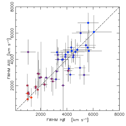
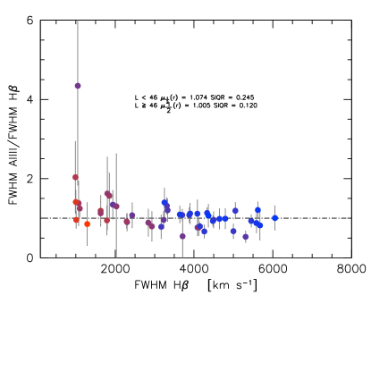
Figure 6: Top panel: FWHM(Aliii) vs. FWHM(H$\beta$) for the joint sample. Data points are color-coded according to luminosity at 1700 Å, from red (lowest; $\log L_{1700}\sim 44$) to blue (highest, $\log L_{1700}\sim 47$). Bottom panel: FWHM ratio of Aliii and H$\beta$. The median ratios $\mu_{\frac{1}{2}}{r}$ and the SIQR ${r}$ are reported for more luminous ($\log L\geq\ 46$  [erg/s]) and less luminous ($\log L<46$) quasars.

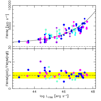
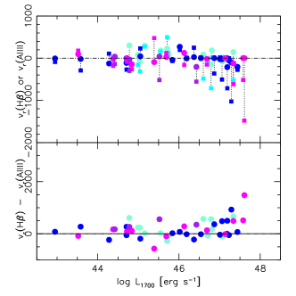
Figure 7: H$\beta$ and Aliii profile parameter comparison as a function of luminosity. Left panel: behavior of FWHM Aliii and H$\beta$  (upper half) and of the ratio FWHM(Aliii)/FWHM(H$\beta$) as a function of $\log L$ at 1700 Å. The filled line traces the expected increase of the FWHM in a virialized system with $L^{\frac{1}{4}}$. The data point are identified on the basis of spectral type as in Fig. 3. The yellow band marks the region where FWHM(Aliii)/FWHM(H$\beta$)=1 within the errors: the median value of the uncertainty of the ratios, $\approx\pm$25%. Right panels: shifts of H$\beta$  and Aliii (upper half), and their difference $s^{\star}$ as a function of $\log L$(1700) (lower half). The vertical dotted lines join H$\beta$ and Aliii parameters for the same object (e.g., they are not error bars).

4.4.2 Shift

The blueshifts involve radial velocities that are relatively modest (right panel of Fig. 7). Aliii shifts exceed 1000 km s^-1 only in two cases of extreme luminosity. Even if we see some increase toward higher $s$ values in the highest luminosity range, several high-luminosity sources remain unshifted within the uncertainties. If we consider the dependence of shifts on luminosity, at high $L$ there is an increase in the range of blueshifts involving values that are relatively large (several hundred km s^-1; Fig. 7). The parameter $\delta$ as a function of $L$ has a more erratic behaviour (Fig. 8), but only at the highest $L\textsterling$ $\delta\approx-0.1$, and the effect of the line shift is at a 10% level. Fig. 8 is consistent with Aliii blueshifts becoming more frequent and of increasing amplitude with luminosity.

Figure 8: Parameter $\delta$(Aliii) as a function of luminosity. Median values are plotted for 1 dex luminosity intervals. Error bars are sample SIQR.

4.5 FWHM H$\beta$ and FWHM Ciii]

The Ciii] line has been considered as a possible virial broadening estimator, and has been a target of reverberation mapping monitoring (Trevese et al., 2007, 2014; Lira et al., 2018; Kaspi et al., 2021). The problem in Population A is that Ciii] shows a strong gradient in its intensity. In spectral type A1, Ciii] is by far the strongest line in the 1900 Å blend, but its prominence decreases with increasing $R_{\rm FeII}$, i.e., going toward spectral type A3 (Bachev et al., 2004). In spectral types A3 and A4 Ciii] is affected by the severe blending with Siiii] and Feiii emission (much more severe than for Aliii), and may become so weak to the point of being barely detectable or even undetectable  (Vestergaard & Wilkes, 2001; Negrete et al., 2014; Temple et al., 2020; Bachev et al., 2004; Martínez-Aldama et al., 2018). In addition, the Ciii] line has a rather low critical density, and its intensity is exposed to the vagaries of density and ionization fluctuations much more than Aliii, whose emission is highly efficient in dense gas over a broad range of ionization levels (Marziani et al., 2020, and Sect. 5.3). The measurements of the Ciii]  width might be inaccurate in extreme Population A if Feiii contamination is strong. It is therefore legitimate to expect a greater dispersion in the width relation of Ciii] with H$\beta$.

The FWHM of Ciii] is shown against the FWHM of H$\beta$ full profile in Fig. 9, upper panel. Error bars show uncertainties computed following the prescription of Appendix A. Not surprisingly, the scatter in the FWHM ratio between Ciii] and H$\beta$ is larger than in the case of Aliii. The top and middle panels of Fig. 9 show that there is a significant deviation from unity, although for relatively narrow profiles around 2000 km s^-1 the FWHM Ciii]  is close to the 1:1 line. The $\chi_{\nu}^{2}$ is much higher than 1. The bottom panel shows the ratio between FWHM Ciii] and FWHM H$\beta$  color-coded according to Ciii] strength. The limit was set at normalized intensity (roughly equal to equivalent width) $I=$ 10. The trend for sources above this limit implies FWHM Ciii]= $\xi_{\mathrm{CIII]}}$ FWHM $\approx$ 0.77 FWHM H$\beta$.

We didn’t detect any strong difference in the trend with luminosity of H$\beta$ and Ciii] FWHM, as it has been the case for H$\beta$ and Aliii. The two lines follow a similar trend with luminosity at 1700 Å (Fig. 10). No shift analysis was carried out for Ciii] due to the severe blending with Siiii] and Feiii.

The narrower profile of Ciii] indicates a higher distance from the central continuum source than the one obtained from H$\beta$, if the velocity field is predominantly virial (Peterson & Wandel, 2000). This result is also consistent with the findings of Negrete et al. (2013) who, using Ciii] intensity ratios in a photoionization estimate of the emitting region radius, obtained much larger radii than the ones obtained from reverberation mappings of H$\beta$.

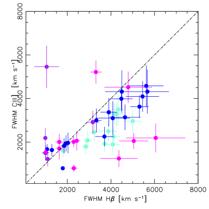
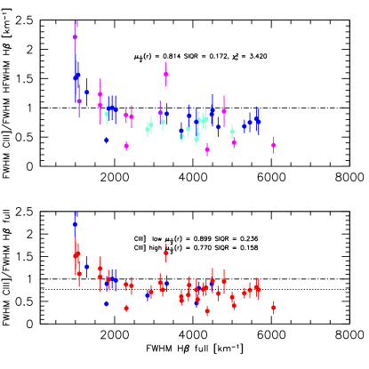
Figure 9: Top panel: FWHM(Ciii]) vs. FWHM(H$\beta$) for the joint sample. Data points are color-coded according to spectral types, as for Fig. 3. Middle panel: FWHM ratio of Ciii] and H$\beta$, The median ratio $\mu_{\frac{1}{2}}({r})$, with $r=$ FWHM Ciii]/FWHM H$\beta$, and the SIQR are reported. Bottom panel: same ratio with the data color-coded according to Ciii] intensity: normalized intensity $>10$ (red) and $\leq 10$ (blue). Values of $\mu_{\frac{1}{2}}({r})$ and SIQR are reported for stronger and weaker Ciii]  emitters.

Figure 10: H$\beta$ and Ciii] profile parameter comparison as a function of luminosity. Top panel: Behavior of FWHM Ciii] and H$\beta$  (upper half) and of the ratio FWHM(Ciii])/FWHM(H$\beta$) as a function of $\log L$ at 1700 Å. The data point are color-coded on the basis of spectral type. As in Fig. 7, the filled line traces the expected increase of the FWHM in a virialized system with $L^{\frac{1}{4}}$. The yellow band marks the region where FWHM(Civ$\lambda$1549)/FWHM(H$\beta$) $\approx$ 0.8 within the errors. The width of the band has been set by the median value of the uncertainty of the ratios, $\pm$ 0.17. The vertical dotted lines join H$\beta$ and Aliii parameters for the same object.

4.6 A $M_{\rm BH}$ scaling law based on Aliii

The goal is to obtain an $M_{\rm BH}$ estimator based on Aliii that is consistent with the scaling law derived for H$\beta$. In this context, the process is much simpler than in the case of Civ$\lambda$1549, where large blueshifts introduced a significant correction and a second-order dependence on luminosity of FWHM Civ$\lambda$1549 could not be bypassed. The H$\beta$ and Aliii widths of the two lines grow in a similar trend with $L$ (Fig. 7). The $M_{\rm BH}$ scaling law can be derived in the form $\log M_{\mathrm{BH}}=\alpha\cdot\log L+2\cdot\log\mathrm{FWHM}+\gamma$ by minimizing the scatter and any systematic deviation of $M_{\rm BH}$  estimated from Aliii with respect to the H$\beta$-derived masses from the Vestergaard & Peterson (2006) scaling law:

$$\log M_{\mathrm{BH}}\,(\mathrm{H\beta})\approx 0.5\log L_{5100,44}+2\log\left(\mathrm{FWHM}(\mathrm{H\beta})\right)+0.91,$$ (3)

where $L_{5100,44}$ is the rest frame luminosity $\lambda L_{\lambda}$ at 5100 Å in units of $10^{44}$ erg  s^-1, and the FWHM H$\beta$ is in km s^-1, considering that no correction is needed to FWHM Aliii  (i.e., $\xi_{\mathrm{AlIII}}\approx 1$). The Vestergaard & Peterson (2006) scaling law is a landmark that has been applied in hundreds of quasar studies. However, the Vestergaard & Peterson (2006) H$\beta$ scaling law provides individual estimates with large error bars in relative estimates ($\approx$0.5 dex at 1$\sigma$, see the discussion in their paper). This is a limit to the precision of any scaling law based on the match with the one based on H$\beta$. The large error bars of individual mass estimates can be mainly explained on the basis of orientation effects (M19) and of trends along the spectral types of the main sequence (Du & Wang, 2019).

If this condition is enforced, the relation between $M_{\rm BH}$ from Aliii and from H$\beta$  (Fig. 11) can be written as:

$$\log M_{\mathrm{BH}}(\mathrm{AlIII})\approx(1.000\pm 0.043)\log M_{\mathrm{BH}}(\mathrm{H\beta})-(0.001\pm 0.367).$$ (4)

The Aliii scaling law takes the form, with the FWHM in km s^-1:

$$\log M_{\mathrm{BH}}\,(\mathrm{AlIII}) \approx (0.579^{+0.031}_{-0.029})\log L_{1700,44}+$$

$$2\log\left(\mathrm{FWHM}(\mathrm{AlIII})\right)+(0.490^{+0.110}_{-0.060}),$$

with an rms scatter $\sigma\approx 0.29$. Figure 11 suggests the presence of a well-behaved distribution with a few outlying points. The relation of Eq. 4.6 considers the FWHM of 47 sources. One data point has been excluded applying a $\sigma$ clipping algorithm (the one A4 outlier, HE0132-4313 (catalog )). This selective procedure is justified by the fact that only some of the most extreme sources of Population A (not all of them) show large blueshifts and only one (HE0132-4313 (catalog )) a FWHM in excess to H$\beta$ by a large factor, deviating at more than 3 times the sample rms. Removal of HE0132-4313 (catalog ) provides however only a minor, not significant change in the fitting parameters. The scaling law parameter uncertainties have been estimated computing the coefficients $\alpha$ and $\gamma$ over a wide range of values and defining the interval where agreement between $M_{\rm BH}$ from H$\beta$ and Aliii (Eq. 4) is satisfied within 1.00$\pm 1\sigma$ for the best-fitting slope and $0.00\pm 1\sigma$ for the intercepts (respectively $\approx$0.043 and $\approx$0.367, as per Eq. 4). Due to some scatter in FWHM relation at FWHM H$\beta_{\rm BC}$  $\sim$ 1000 km s^-1 and the possibility of predominantly face-on orientation (Mejía-Restrepo et al., 2018a) the $M_{\rm BH}$ estimates at $M_{\rm BH}$ $\lesssim 10^{7}$ M_⊙ should be viewed with care due to the paucity of data points.

It is important to remark that this result, unlike the one on Civ$\lambda$1549 $M_{\rm BH}$ estimates, is obtained without any correction on the measured FWHM. The Aliii and H$\beta$ relation should be considered equivalent with respect to $M_{\rm BH}$ estimates in large samples of Population A sources. No scaling law $r_{\mathrm{BLR}}-L$ has been ever derived from reverberation mapping on the Aliii lines. However, it is reassuring that the luminosity exponent ($\approx 0.579^{+0.031}_{-0.029}$) deviates by about $1\sigma$ from the one entering the scaling law $r_{\mathrm{BLR}}-L$ derived by Bentz et al. (2013) for H$\beta$.

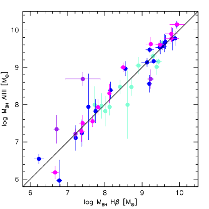
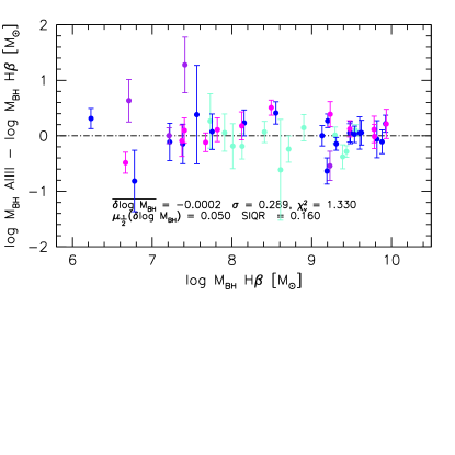
Figure 11: Decimal logarithm of black hole mass in units of solar masses computed from the relation of Vestergaard & Peterson (2006) based on FWHM H$\beta$ vs. the one computed from the Aliii FWHM following Eq. 4.6, with sub-samples identified by color according to their spectral types. The filled line traces Eq. 4, while the dot-dashed line is the equality line. The bottom panel shows the residuals as a function of the $M_{\rm BH}$ derived from H$\beta$. Average values of the $\log$ $M_{\rm BH}$ differences, standard deviation and normalized $\chi_{\nu}^{2}$ are reported for the joint sample minus one outlier with $\delta>1$  (top row). The bottom rows yields the median and the SIQR.

4.7 A $M_{\rm BH}$ scaling law based on Ciii]

An approach analogous to the one adopted for Aliii was also applied to Ciii]. The goal is to obtain an $M_{\rm BH}$ estimator based on Ciii] that is consistent with the scaling law derived for H$\beta$. The process is again much simpler than in the case of Civ$\lambda$1549, where large blueshift introduced a significant correction and a second-order dependence on luminosity of FWHM Civ$\lambda$1549 could not be bypassed. Considering that only a very simple correction is needed to FWHM Ciii], $\xi_{\mathrm{CIII]}}\approx 1.25$, the $M_{\rm BH}$ scaling law can be derived in the form $\log M_{\mathrm{BH}}=\alpha\cdot\log L+2\cdot\log{\xi_{\mathrm{CIII]}}}\mathrm{FWHM}+\gamma$ by minimizing the scatter and any systematic deviation of $M_{\rm BH}$  estimated from Ciii] with respect to the H$\beta$-derived masses. Figure 12 suggests the presence of a well-behaved distribution with a few outlying points. The condition

$$M_{\mathrm{BH}}(\mathrm{CIII]})\approx(1.000\pm 0.053)M_{\mathrm{BH}}(\mathrm{H\beta})+(0.000\pm 0.454)$$ (6)

is satisfied if the Ciii] scaling law takes the form:

$$\log M_{\mathrm{BH}}\,\mathrm{CIII]} \approx (0.6765\pm 0.0450)\log L_{1700,44}+$$

$$2\log\left({\xi_{\mathrm{CIII]}}}\mathrm{FWHM}(\mathrm{CIII]})\right)+(0.332\pm 0.120),$$

with an rms scatter $\sigma\approx 0.35$ (excluding 1 outlier, for 44 objects). The scaling law parameter uncertainties have been estimated varying the coefficients $\alpha$ and $\gamma$ as for the Aliii case.

The $M_{\rm BH}$ Ciii] scaling law is derived with a simple correction on the measured FWHM Ciii]. The Ciii] and H$\beta$ relation should be considered equivalent with respect to $M_{\rm BH}$ estimates in large samples of Population A sources. Care should however be taken to consider sources in which Ciii] can be measured ($W\gtrsim 10$Å) and to identify extreme objects, as discussed in Section 5.3. In addition, the heterogeneity of the sample and the possibility of different trends in different FWHM domains (FWHM (Ciii]) $\approx$ FWHM(H$\beta$) if FWHM $\lesssim$ 3000 km s^-1) makes the scaling law with Aliii  more reliable.

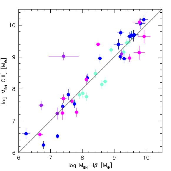
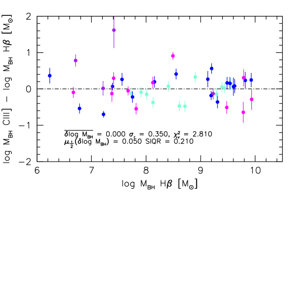
Figure 12: Decimal logarithm of black hole mass in units of solar masses computed from the relation of Vestergaard & Peterson (2006) based on the H$\beta$ spectral range vs. the one computed from the Ciii] data following Eq. 4.7, with spectral types color-coded as in Fig. 3. As for Fig. 11, the filled line traces Eq. 6, while the dot-dashed line is the equality line. The lower panel shows residuals as a function of $M_{\rm BH}$ derived from H$\beta$. Average, standard deviation, and $\chi_{\nu}^{2}$ of the $\log$ $M_{\rm BH}$ difference are reported on the top-row of the inside caption; the bottom row reports median and SIQR.

5 Discussion

Figure 13: Decimal logarithm of black hole mass in units of solar masses computed from the scaling law based on FWHM Ciii] (Eq. 4.7) vs. the one computed from the Aliii FWHM following Eq. 4.6. The filled line traces an unweighted least square fit; the dot-dashed line is the equality line.

In the following we first compare the scaling laws obtained for Aliii and Ciii](Sect. 5.1). The present work detects systematic shifts of Aliii toward the blue. Even if they are on average slightly above the uncertainties, it is interesting to analyze them in the context of systematic shifts affecting the prominent high and low-ionization lines of Civ$\lambda$1549 and Mgii$\lambda$2800 (Section 5.2), and to consider more in detail sources in the spectral type where Aliii are broader than the H$\beta$ ones (Section 5.3).

5.1 Consistency of scaling laws

The scaling laws derived for Aliii and Ciii] are mutually consistent. Black hole mass estimates are shown in Fig. 13. An unweighted lsq fit yields slope $0.975\pm 0.043$, consistent with unity, and intercept $0.246\pm 0.371$, with an rms scatter $\approx$ 0.302. The median difference of the mass values obtained with the two scaling laws is $\mu(\log M_{\mathrm{BH}}\mathrm{(CIII])}-\log M_{\mathrm{BH}}\mathrm{(AlIII)})\approx 0.06\pm 0.20$ (SIQR).

The $r_{\mathrm{BLR}}-L$ implicit in Eq. 6 is consistent with the $r_{\mathrm{BLR}}-L$ relation derived for Civ$\lambda$1549 in a previous study (Trevese et al., 2014), and only slightly higher than the one derived in the early study of Kaspi et al. (2007, $\alpha\approx 0.52-0.55$, c.f. ). More high S/N spectroscopic observations, including monitoring, should be carried out to explore the full potential of the 1900 Å blend lines and especially of Ciii]  as VBEs.

The scaling law derived from the Aliii line is consistent with the Civ$\lambda$1549-based scaling law (M19): Fig. 14 indicates only a slight bias (less than the SIQR $\approx$ 0.2 dex, and the rms $\approx$ 0.3 dex), as the Civ$\lambda$1549 scaling law apparently overestimates the $M_{\rm BH}$ by $\approx 20$% and $\approx 40$% with respect to the $M_{\rm BH}$ estimates based on Aliii and H$\beta$, respectively. Considering that the Civ$\lambda$1549-based scaling law requires a large correction ($\xi_{\mathrm{CIV}}$ can be as low as $\approx$ 0.2) to the Civ$\lambda$1549 FWHM dependent on both line shift and luminosity, the Aliii scaling law should be preferred in case observations of both Civ$\lambda$1549 and Aliii are available.

Figure 14: Decimal logarithm of black hole mass in units of solar masses computed from the Civ$\lambda$1549-based scaling law of M19 vs the ones computed from the relation of Vestergaard & Peterson (2006) based on FWHM H$\beta$ (blue) and from the Aliii FWHM following Eq. 4.6 (black). The dot-dashed is the equality line. The bottom panel shows the residuals as a function of $M_{\rm BH}$. Median and SIQR of the $\log$ $M_{\rm BH}$ differences $\delta\log M_{\mathrm{BH}}=\log M_{\mathrm{BH}}$ CIV $-\log M_{\mathrm{BH}}$ Aliii and $\delta\log M_{\mathrm{BH}}=\log M_{\mathrm{BH}}$ CIV $-\log M_{\mathrm{BH}}$ H$\beta$  are reported in the inside caption.

5.2 Shifts of Aliii vs shifts of Civ$\lambda$1549 and Mgii$\lambda$2800

Fig 15 shows the Aliii peak shifts reported in Table 2 vs. the centroid at half maximum of Civ$\lambda$1549 from S07, S17, Deconto-Machado et al. (2022, in preparation), and the “peak” shift given by Vietri et al. (2018) for the four subsamples of the present work. The Aliii shift is usually very modest, and a factor of $\sim 10$  lower than the shift measured for Civ$\lambda$1549. The Aliii and Civ$\lambda$1549 shifts are however significantly correlated (Pearson’s correlation coefficient $\approx 0.54$, with a significance $P\approx 1.-2\cdot 10^{-3}$):

$$s(\mathrm{AlIII})\approx(0.114\pm 0.026)c({\frac{1}{2}})(\mathrm{CIV})+(50.0\pm 68.5)\mathrm{km\ s^{-1}}.$$ (8)

Figure 15: Shift $s$ of Aliii  vs shift of Civ$\lambda$1549 with respect to rest frame. Data points are identified according to the spectral type, with the same color code of Fig. 3. The filled and dot-dashed lines trace an unweighted least square fit and the equality line, respectively. The grey bands identify uncertainties ranges in radial velocity $\pm 400$km s^-1 where the lines are not significantly shifted. Squares refer to the c($\frac{1}{2}$) Aliii in the case the excess emission on the blue side of Aliii has been ascribed to Aliii. See Section 5.3. 

The slope is shallow, but the correlation indicates that the shifts in Aliii and Civ$\lambda$1549 are likely to be due to the same physical effect. If we ascribe the small displacements observed in the peak shift $s$ of Aliii to the effect of outflows, the outflow prominence is much lower than in the case of Civ$\lambda$1549, both in terms of radial velocity values and of $\delta$.

As mentioned, Civ$\lambda$1549 shifts and FWHM are correlated, implying that the broader the line, the higher the shift amplitude becomes (Coatman et al., 2016; Sulentic et al., 2017). The Aliii shows a consistent behavior, but apparently masked by the much lower shift amplitudes; the presence of Aliii  blueshifts appears to be statistically significant at very high luminosity, and for spectral type A3 and A4. When Civ$\lambda$1549 shows large blueshifts i.e., for high $R_{\rm FeII}$ or very high luminosity, the Aliii line becomes broader than H$\beta$ (even if the two lines remain in fair agreement). We see a relation between Aliii line shift and widths: in ST A3 and A4, where shifts are larger, the Aliii FWHM exceeds the one of H$\beta$ (Figure 5).

The Aliii and Civ$\lambda$1549 results on line shifts are also consistent with the ones obtained for Mgii$\lambda$2800. Small amplitude blueshifts of a few hundreds km s^-1 were measured on the full line profile of Mgii$\lambda$2800  (Marziani et al., 2013b). For Mgii$\lambda$2800 the separation of a BLUE component and a symmetric Lorentzian has been possible on median composite spectra because of the high S/N and of the peaky line core of the Mgii$\lambda$2800 line. The same operation is not feasible for individual Aliii profiles that are often significantly affected by noise, and in some cases even barely above noise. The Aliii, Civ$\lambda$1549 and Mgii$\lambda$2800 are all resonance lines that may be subject to selective line-driven acceleration (Murray & Chiang, 1997; Proga, 2007; Risaliti & Elvis, 2010). The different velocity amplitudes most likely reflect the difference in the line emitting region distance from the continuum source and in physical properties, such as ionization parameter, density and column density.

Rare sources with large shift amplitudes in Aliii are expected to be intrinsically infrequent even at the redshift where luminous quasars were fairly common ($z\approx 1.5-2$) and, even if over-represented because of a Malmquist-type bias, they are outstanding and pretty easily recognizable, especially in large samples of AGN (Sect. 5.3). The most striking case directly resembling Civ$\lambda$1549 is the one of HE0132-4313 (catalog )  which is an object of fairly low luminosity and an outlier in the plots FWHM Aliii vs FWHM H$\beta$. Sources with large shift amplitude may be excluded or flagged if black hole mass estimates are being carried out.

5.3 xA quasars

There are 16 sources meeting the criterion $R_{\rm FeII}$$\gtrsim 1$ in the joint sample. The wide majority of these sources shows Aliii blueshift with respect to H$\beta$. The average shift is rather modest, $\approx-250$ although for 7 of them, $s\lesssim-250$ km s^-1. Six objects show evidence of a strong excess on the blue side of the 1900 blend. Fits to the 1900 blend of these sources following the standard approach are shown in Appendix B. The fits have been repeated by allowing for an extra BLUE in the 1900 blend, represented as a skewed Gaussian (Fig. 16). The blueshifted excess in some cases cannot be distinguished from strong Siii$\lambda$1816 emission. The Siii$\lambda$1816 emission line can be of strength comparable to Aliii in the condition of low ionization and high density derived for the virialized component (Negrete et al., 2012).

In two cases (e.g., HE0359-3959 (catalog ),and SDSS J152156.48+520238.5 (catalog )) the blueshifted excess is so overwhelming that Siii$\lambda$1816 emission cannot account for the excess unless the Siii$\lambda$1816 line itself is significantly blueshifted. These are perhaps the best cases supporting the evidence for a significant BLUE in Aliii. It is reasonable to assume that the blueshifted excess is mainly due to Aliii, being Aliii a resonant line for which BALs are also observed. Broad absorption components are observed in the Aliii profile, even if rarely, and with terminal radial velocity of the absorption through much lower than the one of Civ$\lambda$1549 (Gibson et al., 2009).

The Eddington ratio values derived from the continuum luminosity at 1700 Å (after Galactic extinction correction) multiplied by a bolometric correction factor $k_{\mathrm{bol}}\approx$ 3.5, and from the $M_{\rm BH}$ estimated from Eq. 4.6 range between $L/L_{\rm Edd}$$\approx 0.2$ and $L/L_{\rm Edd}$$\approx 1.5$. If the luminosity-dependent $k_{\mathrm{bol}}$ is applied to the 1700 Å  continuum, $0.2\lesssim$$L/L_{\rm Edd}$$\lesssim 1.1$. Both estimates confirm that all quasars of the presented sample are within the range expected for Pop. A sources. The xA sources are at the high end of the $L/L_{\rm Edd}$ distribution, with $\mu(\log$$L/L_{\rm Edd}$)$\approx-0.18$, and the Aliii BLUE sources are even more extreme with $\mu(\log$$L/L_{\rm Edd}$)$\approx-0.105$. Extreme radiation forces may make it possible to blow out rather dense/high column density gas from the virialized region associated with the emission of the low- and intermediate ionization lines (Netzer & Marziani, 2010). Sources showing a strong BLUE in Aliii could be the most extreme accretors, perhaps in a particular “blow-out” phase of the quasar evolution (D’Onofrio & Marziani, 2018).

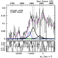
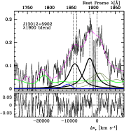
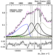
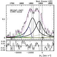
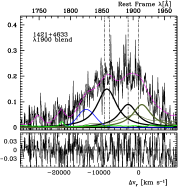
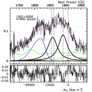
Figure 16: Analysis of the 1900 Å blend for the estreme Population A sources with excess emission on the blue side of Aliii. Abscissa scales are rest-frame wavelength in Å and radial velocity from rest frame wavelength of Ciii]. Ordinate scale is normalized specific flux by the value at 1700 Å. The black lines identify Aliii, Siiii]. The blueshifted excess BLUE is traced by a thick blue line. Green lines trace the adopted Feii (pale) and Feiii (dark) templates. Note that Ciii] emission is almost absent, as all of the emission on the red side of Siiii] can be ascribed to Feiii.

A related issue is whether sources with a strong blue-shifted component in Aliii can be empirically distinguished from the rest of Pop. A quasars, without resorting to the knowledge of the rest frame. The FWHM of the whole blend (i.e., of the sum of all lines after continuum subtraction) is clearly affected by spectral type: going from A1 to A4 we see an overall decrease of prominence in Ciii], and an increase in Aliii with respect to the other line. The blue-shifted excess should further increase the FWHM of the blend. The parameter

$$\mathcal{A}=\frac{\mathrm{FWHM_{1900}}}{\left(10^{\log(\lambda L_{\lambda})_{1700}-44}\right)^{0.25}}$$ (9)

normalizes the FWHM of the whole blend $\mathrm{FWHM}_{1900}$ (i.e., the sum of all line components) because of the increase of the line width with luminosity by a factor $L^{\frac{1}{4}}$. Fig. 17 shows the distribution of the $\mathcal{A}$ for the sources of ST A1 and A2, A3 and A4, and the 6 quasars for which the 1900 blend was fit with the addition of a blue-shifted excess. The distributions of A1+A2 and A3+A4 are significantly different at a 3$\sigma$ confidence level according to a K-S test. However, there is considerable overlap around $\mathcal{A}\approx 3000$ km s^-1, making it difficult to unambiguously distinguishing between xAs, xAs with blue-shifted excess and other sources.

Figure 17: The distribution of the parameter $\mathcal{A}$, as defined in Sect. 5.3, for three groups of quasars: spectral types A1+A2, A3+A4, and the 6 quasars with a blue shifted excess fit to the 1900 Å blend (Fig. 16).

5.3.1 Consistency of UV and optical classification for extreme Population A

Extreme quasars can be identified by employing selection criteria in the optical and UV (MS14). The consistency of the selection criteria is however little tested, since observations covering both the 1900 Å range and the H$\beta$ one are still rare. In the joint sample most sources with $R_{\rm FeII}$$\gtrsim 1$ also satisfy the UV intensity-ratio conditions Aliii/Siiii]$>0.5$, and Siiii]$>$Ciii]. Figure 18 shows the location of the data points identified according to spectral type (defined by ranges of the optical parameter $R_{\rm FeII}$; A3 and A4 satisfy the condition $R_{\rm FeII}$$\gtrsim$ 1 by definition) in the plane defined by the UV ratios Ciii]/Siiii] vs. Aliii/Siiii]. There are several borderline cases, but only one in which the criteria are not satisfied: J15591+3501 (catalog ) with intensity ratios Ciii]/Siiii]$\approx 2.38\pm 0.45$, and Aliii/Siiii]$\approx 0.33\pm 0.06$. For J14421+3526 (catalog ), the feature at $\approx 1910$ Å is most likely a blend of Feiii and Ciii]. In this case, only an upper limit can be assigned to the Ciii] intensity, and the UV selection criteria may not have been violated. The reason of the discordance for J15591+3501 (catalog ) is not clear. The majority of objects ($\approx 80$%) in Figure 18 supports the equivalence between the two xA selection criteria suggested by MS14. Apart from borderline cases, five A2 sources (4 if we exclude J1421+4633 (catalog ) with $R_{\rm FeII}$$\approx$ 0.99) out of 19 enter the domain of the xA (the grey shaded area of Figure 18). These sources appear to be genuine xA in terms of the UV intensity ratios, but have lower than expected $R_{\rm FeII}$ ($0.5\lesssim$ $R_{\rm FeII}$$\lesssim$ 1). It is intriguing that the four sources all belong to the high-$z$ samples. The possibility of systematic differences as a function of redshift in the relative abundance of iron with respect to carbon and $\alpha$ elements should be further investigated (e.g., Martínez-Aldama et al., 2021, and references therein).

Figure 18: The distribution of xA sources in the plane defined by the intensity ratios Ciii]/Siiii] vs Aliii/Siiii]. The area associated with xA sources is the lower-left shaded box. Sources are color coded according to spectral type as in the previous Figures.

6 Summary and conclusion

The present investigation has shown a substantial equivalence of H$\beta$ and Aliii and Ciii] as virial broadening estimators for Population A quasars, thereby providing a tool suitable for $M_{\rm BH}$ estimates up to $z\lesssim 4$ from observations obtained with optical spectrometers. More in detail, the salient results of the present investigation can be summarized as follows:

• the Aliii and H$\beta$ FWHM are highly correlated and, in the joint sample of 48 Population A sources, can be considered statistically equivalent over 4 orders of magnitude in luminosity (Sections 4.1 and 4.2).

• The FWHM ratio between Aliii and H$\beta$ increases with increasing $R_{\rm FeII}$ or, equivalently, from spectral type A1 to A4 (Sect. 4.3). Extreme Pop. A sources appear to be 20% broader than the sample average, while spectral type A1 20 % narrower than spectral type A2.

• Systematic blueshifts are revealed in Aliii; however, in most cases the amplitude of the blueshifts is modest or smaller than the uncertainties, reaching a sample median for spectral types A3 and A4 of just $\approx-160$ km s^-1 (Sections 4.3 and 4.4).

• The line FWHM of H$\beta$, Aliii and Ciii] increases with luminosity as a function of $L^{\frac{1}{4}}$, as expected for a virial velocity field of the line emitting gas (Sect. 4.5).

• The following scaling law between $M_{\rm BH}$ and luminosity and FWHM Aliii: $\log M_{\mathrm{BH}}\,(\mathrm{AlIII})\approx(0.579^{+0.031}_{-0.029})\log L_{1700,44}+2\log\left(\mathrm{FWHM}(\mathrm{AlIII})\right)+(0.490^{+0.110}_{-0.060})$ (Eq. 4.6 in Sect. 4.6) provides an estimate of $M_{\rm BH}$ with an rms scatter of $\approx$ 0.3 dex with respect to the H$\beta$-derived masses, for $M_{\rm BH}$$\gtrsim 10^{7}$ M_⊙.

• An analogous scaling law has been defined also for Ciii]  (Eq. 4.7 in Sect. 4.7). The measurement of the Ciii] FWHM is however more strongly affected by the severe blending and by the Ciii] weakness in sources with high $R_{\rm FeII}$. The Ciii] scaling law requires a constant correction factor to the FWHM of Ciii], $\xi_{\mathrm{CIII]}}\approx 1.25$. The scaling laws derived from Aliii and Ciii] line width are mutually consistent (Sect. 5.1).

• Although Aliii shift amplitudes are $\approx\frac{1}{10}$ the shifts of Civ$\lambda$1549 (Section 5.2), it is unclear whether Aliii can be exploited as a virial luminosity estimator for extreme Population A sources (Section 5.3): the Aliii profile is strongly affected by a blueshifted excess in several extreme Pop. A sources (Sect. 5.3). The majority of quasars show consistency between FWHM Aliii and H$\beta$, and a minority of sources that show FWHM Aliii$\gg$ FWHM H$\beta$ might be easy to recognize in large samples. The extent of systematic effects should however be analyzed by a thorough study of a very large sample of xA sources with full coverage of the optical and UV rest-frame ranges from 1000 to 5500 Å.

These results show that the Aliii line is a good UV substitute of H$\beta$ and can be used for black hole mass estimations with the advantage to be at the rest-frame of the source. The results on FWHM Aliii  should be compared with the ones obtained for Civ$\lambda$1549 (M19), where the equivalence was obtained at the expense of corrections that were dependent on the accurate knowledge of the quasar rest frame, and therefore not fully achievable without additional measurements in spectral ranges distinct from the one of Civ$\lambda$1549: the [Oii]$\lambda$3727 line is the narrow low ionization line closest in wavelength to Civ$\lambda$1549 and offers a reliable rest frame estimator (Bon et al., 2020), but is very rarely covered along with Civ$\lambda$1549.

Appendix A Estimation of uncertainties

A.1 Bayesian estimates

Uncertainties were estimated following a Bayesian approach, considering the likelihood function

$$\log{\mathcal{L}}\propto-\sum_{i}\frac{(f_{\mathrm{i}}-m_{\mathrm{i}}({\bf\Theta}))^{2}}{2\sigma_{\mathrm{i}}^{2}}\propto-\frac{1}{2}\log\chi^{2},$$ (A1)

where $f_{\mathrm{i}}$ are the specific flux values as a function of wavelength (or of pixel number), $\sigma_{\mathrm{i}}$ the uncertainty in $f_{\mathrm{i}}$ (in practice from the S/N set constant over the spectrum), $m_{\mathrm{i}}({\bf\Theta})$ the expectation value for the multicomponent model ${\bf\Theta}$ of the spectrum obtained via a specfit analysis. The ${\bf\Theta}$ can be any set of free parameters employed in the fits: intensity, shift and width of each line, intensity, shift and width of each template. Priors were specified for several parameters in terms of a range of permitted values. The posteriors of the model parameters ${\bf\Theta}$ (for instance, the distributions of FWHM H$\beta$ and Aliii  given the data) were obtained by creating a random walk with a modified Metropolis-Hasting algorithm: a new candidate set of model parameters ${\bf\Theta}$ was randomly generated, and screened by an accettance parameter $\alpha$. The set ${\bf\Theta}$ included model parameters believed to significantly affect the line widths (in practice, most of the parameters included in the specfit analysis). For example, the [Oiii]$\lambda\lambda$4959,5007 lines were modeled with two components, a “core” component represented by a symmetric Gaussian, and a semi-broad component modeled by a skew Gaussian. The template Feii emission was scaled, shifted and broadened as done in the specfit procedure. The dispersion of the posterior distribution of each spectral parameter was assumed to yield its uncertainty $\delta$ at $1\sigma$ confidence level.

A.2 The quality parameter ${\mathcal{Q}}$

The next step was to connect the uncertainty in FWHM, shift and intensity to a quality parameter ${\mathcal{Q}}$, which may turn useful in case very late samples of quasars are analysed. The quality parameter

$${\mathcal{Q}}=\log_{10}\frac{W}{\mathrm{FWHM}}\cdot{\frac{\mathrm{S}}{\mathrm{N}}}$$ (A2)

defined as the product of the S/N times a line equivalent width $W$ divided by its FWHM, increases with S/N and line prominence over the continuum and decreases with increasing line widths. The signal in each resolution element is proportional to the ratio $W$/FWHM, which is a measurement of the sharpness of the line, as obviously ${\mathcal{Q}}\propto\log_{10}\frac{I_{\mathrm{peak}}\cdot\mathrm{FWHM}}{\mathrm{FWHM}I_{\mathrm{c}}}\cdot{\frac{I_{\mathrm{c}}}{\mathrm{N}}}\propto\frac{I_{\mathrm{peak}}}{\mathrm{N}}$. The quality parameter ${\mathcal{Q}}$ obviates to the inadequacy of the S/N measurement carried out on the continuum. By multiplying it by the ratio $W$/FWHM we compute a more apt average S/N for a line depending on its strength and width. The parameter ${\mathcal{Q}}$ is larger for sharp lines in spectra with high S/N in the continuum. The large differences in S/N, line width and line strength between Aliii and H$\beta$ is reflected in the distribution of the ${\mathcal{Q}}$ parameter, shown in Fig. 19.

To be of any practical use, the ${\mathcal{Q}}$ parameter needs to be anchored to estimates of the uncertainties. The posterior distributions of the spectral parameters were computed for about 30 sources. Fig. 20 shows a well-defined trend between ${\mathcal{Q}}$ and the fractional uncertainty $\delta$FWHM/FWHM for H$\beta$, Aliii, and Ciii] derived from the MCMC simulations. Especially for large ${\mathcal{Q}}$ values, the scatter is relatively modest, and the relation between the parameter FWHM, flux and shift and $\log{\mathcal{Q}}$ can be written in a linear form, save for the fractional uncertainty of FWHM Aliii that is best fit by $\delta\mathrm{FWHM}/\mathrm{FWHM}\approx 1/(a+b\log{\mathcal{Q}})$. Table 3 provides the coefficients $a$ and $b$ of the best fits along with ${\mathcal{Q}}$ domain. The FWHM relations were obtained by a non-linear fit algorithm implemented in R (R Core Team, 2019), and are shown as the thick lines in Fig. 20.

Table 3: Relation between fractional uncertainties and ${\mathcal{Q}}$

Parameter	$a$	$b$	$\log{\mathcal{Q}}$ domain
H$\beta$
FWHM	0.100	–0.125	$\approx-0.8\ldots 0.5$
F	0.0666	–0.07022
Shift	66	-0.112
Aliii
FWHM	10.96	6.15	$\approx-1.6\ldots-0.6$
F	0.061	$-0.2277$
Shift	180	$-219.7$
Ciii]
FWHM	0.160	–0.026	$\approx-2.5\ldots 0.0$
F	$-0.026$	$-0.292$
Feii
F	-0.04755	0.07520	$\approx-0.8\ldots 0.5$

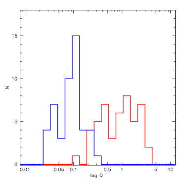
Figure 19: Left: distribution of the $\log$ of parameter ${\mathcal{Q}}$ parameter for Aliii (blue) and H$\beta$ (red) for the joint sample considered in this paper. Right: distribution of $\log{\mathcal{Q}}$  differences between H$\beta$ and Aliii.

Figure 20: Relation between the fractional uncertainty ${\delta\mathrm{FWHM}}/{\mathrm{FWHM}}$ and the logarithm of parameter ${\mathcal{Q}}$. Red spots are for H$\beta$, black for Aliii, blue for Ciii]. The thick lines trace the relations reported in Table 3 for the FWHM of Aliii (black) and Ciii] (blue).

Pollo

Appendix B H$\beta$ and 1900 blend paired comparison

The results of line profile fitting for the 1900 blend and H$\beta$ are shown in the following figures: Fig. 21 for the FOS sample, Fig. 22 for the HE sample, Fig. 23 for the FOS sample, and Fig. 24 for the WISSH sample. All spectra have been continuum subtracted and normalized by the 5100 Å (H$\beta$) and 1700 Å (1900 blend) specific flux.

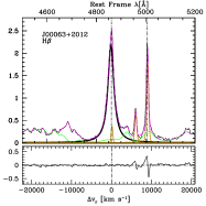
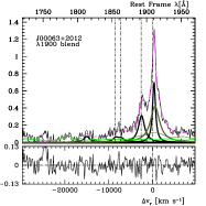
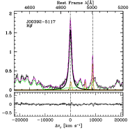
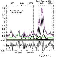
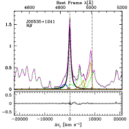
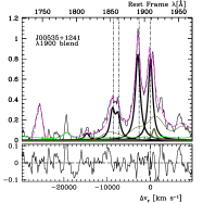
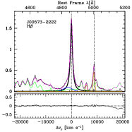
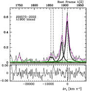
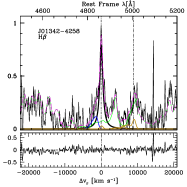
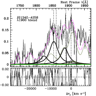
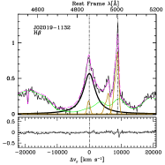
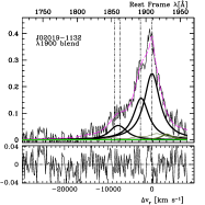
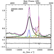
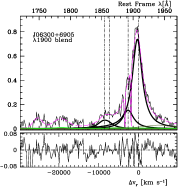
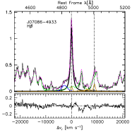
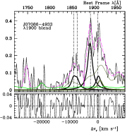
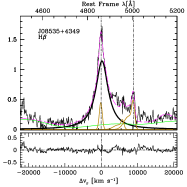
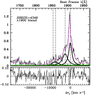
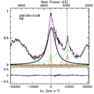
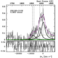
Figure 21: Analysis of the H$\beta$ spectral range (left) and of 1900 Å blend (right), for the sources of the $FOS^{\ast}$ subsample. Abscissa scales are rest-frame wavelength in Å and radial velocity from rest-frame. Ordinate scale is normalized specific flux by the value at 5100 Å and at 1700 Å. The dashed magenta lines trace the sum of all emission components of the model. The black lines identify the H$\beta$ broad component H$\beta_{\rm BC}$ (left), and Aliii, Siiii], and Ciii] (right). The blue line the blueshifted excess in the H$\beta$ profile. Green lines trace the adopted Feii (pale) and Feiii (dark) templates. Golden lines trace narrow emission lines or line components.

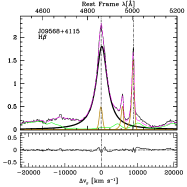
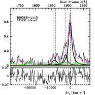
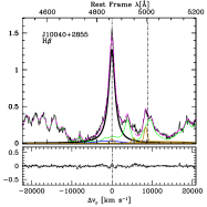
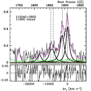
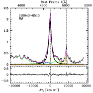
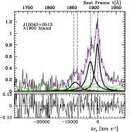
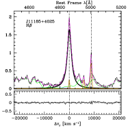
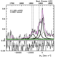
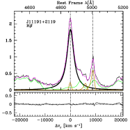
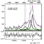
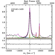
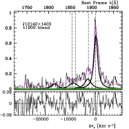
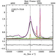
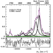
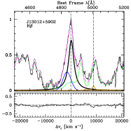
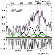
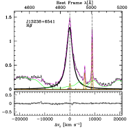
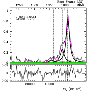
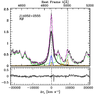
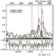
Figure 21: Analysis of H$\beta$ and of the 1900 Å blend for Pop. A sources (cont.).

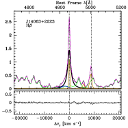
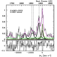
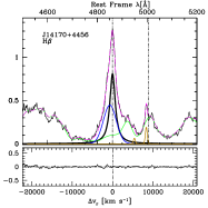
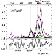
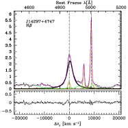
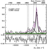
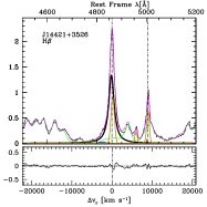
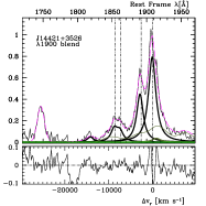
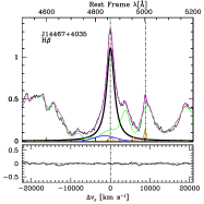
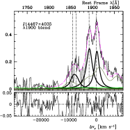
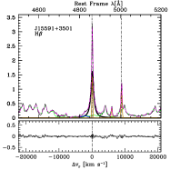
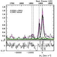
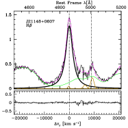
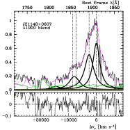
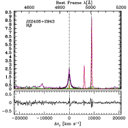
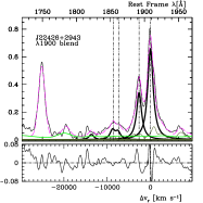
Figure 21: Analysis of H$\beta$ and of the 1900 Å blend for Pop. A sources (cont.).

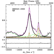
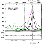
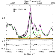
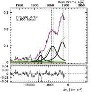
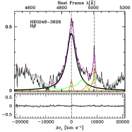
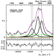
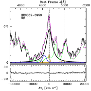
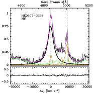
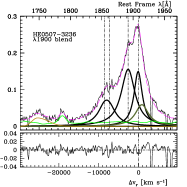
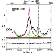
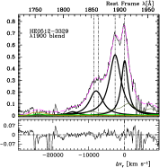
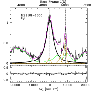
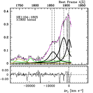
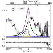
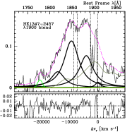
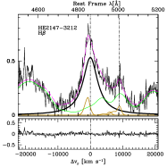
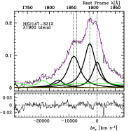
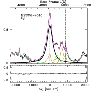
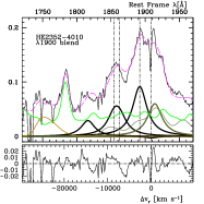
Figure 22: Analysis of the 1900 Å blend, for 10 Pop. A sources of the HE sub-sample. Meaning of color coding is the same as in Fig. 21.

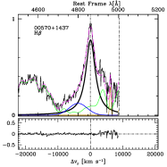
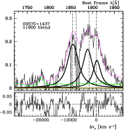
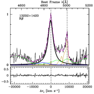
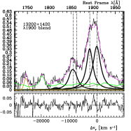
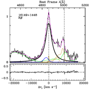
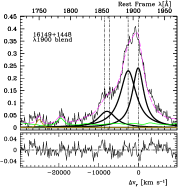
Figure 23: Analysis of H$\beta$ and of the 1900 Å blend for Pop. A sources of the ISAAC sample. Meaning of color coding is the same of the previous Figures in the Appendix.

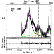
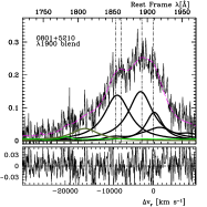
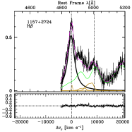
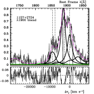
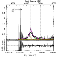
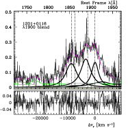
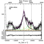
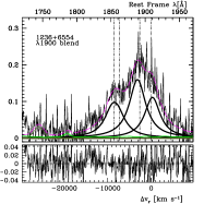
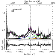
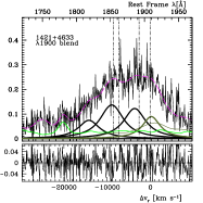
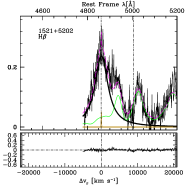
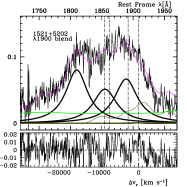
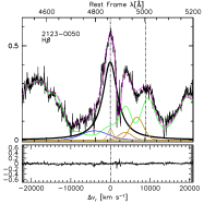
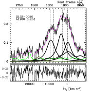
Figure 24: Analysis of H$\beta$ and of the 1900 Å blend for Pop. A sources of the WISSH sample. Meaning of color coding is the same of the previous Figures in the Appendix.

Appendix C Notes on individual objects

J01342-4258

Extreme of extreme Population A. Strong feature at 2080 Å, extreme Feiii emission. In the UV spectrum a strong shelf of emission extends from the red end of the 1900 Å blend to beyond 1950 Å. Inverted radio spectrum not accounted for by the classical synchrotron scenario.

J02019-1132

The CSS source 3C 57 shows a spectrum of Pop. A in the optical range. Analyzed by Sulentic et al. (2015).

HE 0248–3628

Candidate high-frequency peaking object which could be associated with an incerted or self-abosbed spectrum in 5 – 20 GHz frequency domain (Massardi et al., 2016). We speculate that HE 0248–3628 (catalog ) and J01342-4258 (catalog ) could be both objects whose radio emission is not due to a relativistic jet but to thermal sources (Ganci et al., 2019).

J09199+5153

Luminous quasar, considered with “unusually strong optical Feii  emission” (Sulentic et al., 1990). The $R_{\rm FeII}$ $\approx 0.8$ confirms that optical Feii emission is prominent, but not extraordinarily so. The UV spectrum is definitely not xA, and is consistent with the A2 classification based on the optical spectrum.

J07086-4933

Bad spectrum contaminated by heavy absorptions; Aliii lower limit.

HE 0043-2300

Apart from 3C 57, the only source truly “jetted” radio loud.

HE 0359-3959

High-luminosity analogous of J01342-4258; extreme Civ$\lambda$1549 blueshift and extremely low ionization in the virialized BLR (Martínez-Aldama et al., 2017).

J1157+2724

This WISSH source has a significant difference in the redshift estimated for the present work and the one published by Vietri et al. (2018) which is estimated from the narrow H$\beta$ component, 2.2133 vs 2.2170. The difference is significant. The larger redshift of Vietri et al. (2018) would imply larger shifts of Aliii.

References

- Assef et al. (2011) Assef, R. J., Denney, K. D., Kochanek, C. S., et al. 2011, ApJ, 742, 93, doi: 10.1088/0004-637X/742/2/93
- Azzalini & Regoli (2012) Azzalini, A., & Regoli, G. 2012, Ann. Inst. Statist. Math., 64, 857, doi: 10.1007/s10463-011-0338-5
- Bañados et al. (2018) Bañados, E., Venemans, B. P., Mazzucchelli, C., et al. 2018, Nature, 553, 473, doi: 10.1038/nature25180
- Bachev et al. (2004) Bachev, R., Marziani, P., Sulentic, J. W., et al. 2004, ApJ, 617, 171, doi: 10.1086/425210
- Baldwin et al. (2004) Baldwin, J. A., Ferland, G. J., Korista, K. T., Hamann, F., & LaCluyzé, A. 2004, ApJ, 615, 610, doi: 10.1086/424683
- Baldwin et al. (1996) Baldwin, J. A., Ferland, G. J., Korista, K. T., et al. 1996, ApJ, 461, 664, doi: 10.1086/177093
- Barai et al. (2018) Barai, P., Gallerani, S., Pallottini, A., et al. 2018, MNRAS, 473, 4003, doi: 10.1093/mnras/stx2563
- Bentz et al. (2013) Bentz, M. C., Denney, K. D., Grier, C. J., et al. 2013, ApJ, 767, 149, doi: 10.1088/0004-637X/767/2/149
- Bischetti et al. (2017) Bischetti, M., Piconcelli, E., Vietri, G., et al. 2017, A&A, 598, A122, doi: 10.1051/0004-6361/201629301
- Bon et al. (2020) Bon, N., Marziani, P., Bon, E., et al. 2020, A&A, 635, A151, doi: 10.1051/0004-6361/201936773
- Boroson & Green (1992) Boroson, T. A., & Green, R. F. 1992, ApJS, 80, 109, doi: 10.1086/191661
- Brotherton et al. (1994) Brotherton, M. S., Wills, B. J., Steidel, C. C., & Sargent, W. L. W. 1994, ApJ, 423, 131, doi: 10.1086/173794
- Bruhweiler & Verner (2008) Bruhweiler, F., & Verner, E. 2008, ApJ, 675, 83, doi: 10.1086/525557
- Capetti et al. (1996) Capetti, A., Axon, D. J., Macchetto, F., Sparks, W. B., & Boksenberg, A. 1996, ApJ, 469, 554, doi: 10.1086/177804
- Carniani et al. (2015) Carniani, S., Marconi, A., Maiolino, R., et al. 2015, A&A, 580, A102, doi: 10.1051/0004-6361/201526557
- Coatman et al. (2016) Coatman, L., Hewett, P. C., Banerji, M., & Richards, G. T. 2016, MNRAS, 461, 647, doi: 10.1093/mnras/stw1360
- Colbert et al. (1998) Colbert, E. J. M., Baum, S. A., O’Dea, C. P., & Veilleux, S. 1998, ApJ, 496, 786, doi: 10.1086/305417
- Cracco et al. (2016) Cracco, V., Ciroi, S., Berton, M., et al. 2016, MNRAS, 462, 1256, doi: 10.1093/mnras/stw1689
- Decarli et al. (2010) Decarli, R., Falomo, R., Treves, A., et al. 2010, MNRAS, 402, 2441, doi: 10.1111/j.1365-2966.2009.16048.x
- D’Onofrio & Marziani (2018) D’Onofrio, M., & Marziani, P. 2018, Frontiers in Astronomy and Space Sciences, 5, 31, doi: 10.3389/fspas.2018.00031
- Du & Wang (2019) Du, P., & Wang, J.-M. 2019, ApJ, 886, 42, doi: 10.3847/1538-4357/ab4908
- Du et al. (2016) Du, P., Wang, J.-M., Hu, C., et al. 2016, ApJ, 818, L14, doi: 10.3847/2041-8205/818/1/L14
- Everett (2007) Everett, J. E. 2007, Ap&SS, 311, 269, doi: 10.1007/s10509-007-9536-2
- Fabian (2012) Fabian, A. C. 2012, ARA&A, 50, 455, doi: 10.1146/annurev-astro-081811-125521
- Fraix-Burnet et al. (2017) Fraix-Burnet, D., D’Onofrio, M., & Marziani, P. 2017, Frontiers in Astronomy and Space Sciences, 4, 20, doi: 10.3389/fspas.2017.00020
- Ganci et al. (2019) Ganci, V., Marziani, P., D’Onofrio, M., et al. 2019, A&A, 630, A110, doi: 10.1051/0004-6361/201936270
- Gardner et al. (2006) Gardner, J. P., Mather, J. C., Clampin, M., et al. 2006, Space Science Reviews, 123, 485, doi: 10.1007/s11214-006-8315-7
- Gaskell (1982) Gaskell, C. M. 1982, ApJ, 263, 79, doi: 10.1086/160481
- Giannuzzo & Stirpe (1996) Giannuzzo, E. M., & Stirpe, G. M. 1996, A&A, 314, 419
- Gibson et al. (2009) Gibson, R. R., Jiang, L., Brandt, W. N., et al. 2009, ApJ, 692, 758, doi: 10.1088/0004-637X/692/1/758
- Gilmozzi & Spyromilio (2007) Gilmozzi, R., & Spyromilio, J. 2007, The Messenger, 127, 11
- Graham et al. (1996) Graham, M. J., Clowes, R. G., & Campusano, L. E. 1996, MNRAS, 279, 1349
- Grupe et al. (1998) Grupe, D., Beuermann, K., Thomas, H. C., Mannheim, K., & Fink, H. H. 1998, A&A, 330, 25. https://arxiv.org/abs/astro-ph/9710298
- Grupe et al. (2010) Grupe, D., Komossa, S., Leighly, K. M., & Page, K. L. 2010, ApJS, 187, 64, doi: 10.1088/0067-0049/187/1/64
- Heckman & Best (2014) Heckman, T. M., & Best, P. N. 2014, ARA&A, 52, 589, doi: 10.1146/annurev-astro-081913-035722
- Jones et al. (2004) Jones, D. H., Saunders, W., Colless, M., et al. 2004, MNRAS, 355, 747, doi: 10.1111/j.1365-2966.2004.08353.x
- Kakkad et al. (2020) Kakkad, D., Mainieri, V., Vietri, G., et al. 2020, A&A, 642, A147, doi: 10.1051/0004-6361/202038551
- Kaspi et al. (2007) Kaspi, S., Brandt, W. N., Maoz, D., et al. 2007, ApJ, 659, 997, doi: 10.1086/512094
- Kaspi et al. (2021) —. 2021, arXiv e-prints, arXiv:2106.00691. https://arxiv.org/abs/2106.00691
- King & Muldrew (2016) King, A., & Muldrew, S. I. 2016, MNRAS, 455, 1211, doi: 10.1093/mnras/stv2347
- King & Pounds (2015) King, A., & Pounds, K. 2015, ARA&A, 53, 115, doi: 10.1146/annurev-astro-082214-122316
- Komossa et al. (2018) Komossa, S., Xu, D. W., & Wagner, A. Y. 2018, MNRAS, 477, 5115, doi: 10.1093/mnras/sty901
- Kormendy & Ho (2013) Kormendy, J., & Ho, L. C. 2013, Ann. Rev. Astron. Astroph., 51, 511, doi: 10.1146/annurev-astro-082708-101811
- Kriss (1994) Kriss, G. 1994, Astronomical Data Analysis Software and Systems III, A.S.P. Conference Series, 61, 437
- Laurenti et al. (2021) Laurenti, M., Luminari, A., Tombesi, F., et al. 2021, A&A, 645, A118, doi: 10.1051/0004-6361/202039409
- Leighly et al. (2015) Leighly, K. M., Cooper, E., Grupe, D., Terndrup, D. M., & Komossa, S. 2015, ApJ, 809, L13, doi: 10.1088/2041-8205/809/1/L13
- Leighly & Moore (2004) Leighly, K. M., & Moore, J. R. 2004, ApJ, 611, 107, doi: 10.1086/422088
- Lipari et al. (1993) Lipari, S., Terlevich, R., & Macchetto, F. 1993, ApJ, 406, 451, doi: 10.1086/172456
- Lira et al. (2018) Lira, P., Kaspi, S., Netzer, H., et al. 2018, ApJ, 865, 56, doi: 10.3847/1538-4357/aada45
- Lupton & Monger (1996) Lupton, R., & Monger, P. 1996, SM, 2nd edn., McMaster University
- Marinello et al. (2020a) Marinello, M., Rodríguez-Ardila, A., Marziani, P., Sigut, A., & Pradhan, A. 2020a, MNRAS, doi: 10.1093/mnras/staa934
- Marinello et al. (2020b) Marinello, M., Overzier, R. A., Röttgering, H. J. A., et al. 2020b, MNRAS, 492, 1991, doi: 10.1093/mnras/stz3333
- Martínez-Aldama et al. (2017) Martínez-Aldama, M. L., Del Olmo, A., Marziani, P., et al. 2017, Frontiers in Astronomy and Space Sciences, 4, 29, doi: 10.3389/fspas.2017.00029
- Martínez-Aldama et al. (2018) Martínez-Aldama, M. L., del Olmo, A., Marziani, P., et al. 2018, A&A, 618, A179, doi: 10.1051/0004-6361/201833541
- Martínez-Aldama et al. (2021) Martínez-Aldama, M. L., Panda, S., Czerny, B., et al. 2021, arXiv e-prints, arXiv:2101.06999. https://arxiv.org/abs/2101.06999
- Marziani et al. (2020) Marziani, P., del Olmo, A., Perea, J., D’Onofrio, M., & Panda, S. 2020, Atoms, 8, 94, doi: 10.3390/atoms8040094
- Marziani & Sulentic (2012) Marziani, P., & Sulentic, J. W. 2012, NARev, 56, 49, doi: 10.1016/j.newar.2011.09.001
- Marziani & Sulentic (2014) —. 2014, MNRAS, 442, 1211, doi: 10.1093/mnras/stu951
- Marziani et al. (1996) Marziani, P., Sulentic, J. W., Dultzin-Hacyan, D., Calvani, M., & Moles, M. 1996, ApJS, 104, 37, doi: 10.1086/192291
- Marziani et al. (2013a) Marziani, P., Sulentic, J. W., Plauchu-Frayn, I., & del Olmo, A. 2013a, AAp, 555, 89, 16pp. https://arxiv.org/abs/1305.1096
- Marziani et al. (2013b) —. 2013b, ApJ, 764. https://arxiv.org/abs/1301.0520
- Marziani et al. (2003) Marziani, P., Sulentic, J. W., Zamanov, R., et al. 2003, ApJS, 145, 199, doi: 10.1086/346025
- Marziani et al. (2001) Marziani, P., Sulentic, J. W., Zwitter, T., Dultzin-Hacyan, D., & Calvani, M. 2001, ApJ, 558, 553, doi: 10.1086/322286
- Marziani et al. (2017) Marziani, P., Negrete, C. A., Dultzin, D., et al. 2017, in IAU Symposium, Vol. 324, IAU Symposium, 245–246, doi: 10.1017/S1743921316012655
- Marziani et al. (2019) Marziani, P., del Olmo, A., Martínez-Carballo, M. A., et al. 2019, A&A, 627, A88, doi: 10.1051/0004-6361/201935265
- Massardi et al. (2016) Massardi, M., Bonaldi, A., Bonavera, L., et al. 2016, MNRAS, 455, 3249, doi: 10.1093/mnras/stv2561
- Massaro et al. (2009) Massaro, E., Giommi, P., Leto, C., et al. 2009, A&A, 495, 691, doi: 10.1051/0004-6361:200810161
- Mathur (2000) Mathur, S. 2000, MNRAS, 314, L17, doi: 10.1046/j.1365-8711.2000.03530.x
- McLure & Dunlop (2004) McLure, R. J., & Dunlop, J. S. 2004, MNRAS, 352, 1390, doi: 10.1111/j.1365-2966.2004.08034.x
- McLure & Jarvis (2002) McLure, R. J., & Jarvis, M. J. 2002, MNRAS, 337, 109, doi: 10.1046/j.1365-8711.2002.05871.x
- Mejía-Restrepo et al. (2018a) Mejía-Restrepo, J. E., Lira, P., Netzer, H., Trakhtenbrot, B., & Capellupo, D. M. 2018a, Nature Astronomy, 2, 63, doi: 10.1038/s41550-017-0305-z
- Mejía-Restrepo et al. (2018b) Mejía-Restrepo, J. E., Trakhtenbrot, B., Lira, P., & Netzer, H. 2018b, MNRAS, doi: 10.1093/mnras/sty1086
- Mejía-Restrepo et al. (2016) Mejía-Restrepo, J. E., Trakhtenbrot, B., Lira, P., Netzer, H., & Capellupo, D. M. 2016, MNRAS, 460. https://arxiv.org/abs/1603.03437
- Murray & Chiang (1997) Murray, N., & Chiang, J. 1997, ApJ, 474, 91, doi: 10.1086/303443
- Nardini et al. (2019) Nardini, E., Lusso, E., Risaliti, G., et al. 2019, A&A, 632, A109, doi: 10.1051/0004-6361/201936911
- Negrete et al. (2012) Negrete, A., Dultzin, D., Marziani, P., & Sulentic, J. 2012, ApJ, 757, 62. https://arxiv.org/abs/1107.3188
- Negrete et al. (2018) Negrete, C. A., Dultzin, D., Marziani, P., & et al. 2018, in preparation
- Negrete et al. (2013) Negrete, C. A., Dultzin, D., Marziani, P., & Sulentic, J. W. 2013, ApJ, 771, 31, doi: 10.1088/0004-637X/771/1/31
- Negrete et al. (2014) —. 2014, ApJ, 794, 95, doi: 10.1088/0004-637X/794/1/95
- Netzer et al. (2007) Netzer, H., Lira, P., Trakhtenbrot, B., Shemmer, O., & Cury, I. 2007, ApJ, 671, 1256, doi: 10.1086/523035
- Netzer & Marziani (2010) Netzer, H., & Marziani, P. 2010, ApJ, 724, 318, doi: 10.1088/0004-637X/724/1/318
- O’Dea (1998) O’Dea, C. P. 1998, PASP, 110, 493, doi: 10.1086/316162
- Oliphant (2015) Oliphant, T. 2015, NumPy: A guide to NumPy, 2nd edn., USA: CreateSpace Independent Publishing Platform. http://www.numpy.org/
- Padovani (2017) Padovani, P. 2017, Frontiers in Astronomy and Space Sciences, 4, 35, doi: 10.3389/fspas.2017.00035
- Panda et al. (2018) Panda, S., Czerny, B., Adhikari, T. P., et al. 2018, The Astrophysical Journal, 866, 115, doi: 10.3847/1538-4357/aae209
- Panda et al. (2019) Panda, S., Marziani, P., & Czerny, B. 2019, arXiv e-prints, arXiv:1905.01729. https://arxiv.org/abs/1905.01729
- Peterson (2014) Peterson, B. M. 2014, SpScieRev, 183, 253, doi: 10.1007/s11214-013-9987-4
- Peterson & Wandel (1999) Peterson, B. M., & Wandel, A. 1999, ApJ, 521, L95, doi: 10.1086/312190
- Peterson & Wandel (2000) —. 2000, ApJ, 540, L13, doi: 10.1086/312862
- Peterson et al. (2004) Peterson, B. M., Ferrarese, L., Gilbert, K. M., et al. 2004, ApJ, 613, 682, doi: 10.1086/423269
- Popović et al. (2019) Popović, L. Č., Kovačević-Dojčinović, J., & Marčeta-Mand ić, S. 2019, MNRAS, 484, 3180, doi: 10.1093/mnras/stz157
- Press et al. (1992) Press, W. H., Teukolsky, S. A., Vetterling, W. T., & Flannery, B. P. 1992, Numerical recipes in FORTRAN. The art of scientific computing (Cambridge University Press)
- Proga (2007) Proga, D. 2007, in Astronomical Society of the Pacific Conference Series, Vol. 373, The Central Engine of Active Galactic Nuclei, ed. L. C. Ho & J.-W. Wang, 267
- R Core Team (2019) R Core Team. 2019, R: A Language and Environment for Statistical Computing, R Foundation for Statistical Computing, Vienna, Austria. https://www.R-project.org/
- Richards et al. (2011) Richards, G. T., Kruczek, N. E., Gallagher, S. C., et al. 2011, AJ, 141, 167, doi: 10.1088/0004-6256/141/5/167
- Risaliti & Elvis (2010) Risaliti, G., & Elvis, M. 2010, A&A, 516, A89, doi: 10.1051/0004-6361/200912579
- Shen (2013) Shen, Y. 2013, Bulletin of the Astronomical Society of India, 41, 61. https://arxiv.org/abs/1302.2643
- Shen & Ho (2014) Shen, Y., & Ho, L. C. 2014, Nature, 513, 210, doi: 10.1038/nature13712
- Shen & Liu (2012) Shen, Y., & Liu, X. 2012, ApJ, 753, 125, doi: 10.1088/0004-637X/753/2/125
- Smee et al. (2013) Smee, S. A., Gunn, J. E., Uomoto, A., et al. 2013, AJ, 146, 32, doi: 10.1088/0004-6256/146/2/32
- Śniegowska et al. (2018) Śniegowska, M., Kozowski, S., Czerny, B., & Panda, S. 2018, arXiv e-prints, arXiv:1810.09363. https://arxiv.org/abs/1810.09363
- Sulentic et al. (2011) Sulentic, J., Marziani, P., & Zamfir, S. 2011, Baltic Astronomy, 20, 427
- Sulentic et al. (2007) Sulentic, J. W., Bachev, R., Marziani, P., Negrete, C. A., & Dultzin, D. 2007, ApJ, 666, 757, doi: 10.1086/519916
- Sulentic et al. (1990) Sulentic, J. W., Calvani, M., Marziani, P., & Zheng, W. 1990, ApJ, 355, L15, doi: 10.1086/185727
- Sulentic et al. (2015) Sulentic, J. W., Martínez-Carballo, M. A., Marziani, P., et al. 2015, MNRAS, 450, 1916, doi: 10.1093/mnras/stv710
- Sulentic et al. (2000a) Sulentic, J. W., Marziani, P., & Dultzin-Hacyan, D. 2000a, ARA&A, 38, 521, doi: 10.1146/annurev.astro.38.1.521
- Sulentic et al. (2002) Sulentic, J. W., Marziani, P., Zamanov, R., et al. 2002, ApJL, 566, L71, doi: 10.1086/339594
- Sulentic et al. (2000b) Sulentic, J. W., Marziani, P., Zwitter, T., Dultzin-Hacyan, D., & Calvani, M. 2000b, ApJL, 545, L15, doi: 10.1086/317330
- Sulentic et al. (2004) Sulentic, J. W., Stirpe, G. M., Marziani, P., et al. 2004, A&Ap, 423, 121, doi: 10.1051/0004-6361:20035912
- Sulentic et al. (2017) Sulentic, J. W., del Olmo, A., Marziani, P., et al. 2017, A&A, 608, A122, doi: 10.1051/0004-6361/201630309
- Temple et al. (2020) Temple, M. J., Ferland, G. J., Rankine, A. L., et al. 2020, MNRAS, 496, 2565, doi: 10.1093/mnras/staa1717
- Trakhtenbrot & Netzer (2012) Trakhtenbrot, B., & Netzer, H. 2012, MNRAS, 427, 3081, doi: 10.1111/j.1365-2966.2012.22056.x
- Trakhtenbrot et al. (2015) Trakhtenbrot, B., Urry, C. M., Civano, F., et al. 2015, Science, 349, 168, doi: 10.1126/science.aaa4506
- Trevese et al. (2007) Trevese, D., Paris, D., Stirpe, G. M., Vagnetti, F., & Zitelli, V. 2007, A&A, 470, 491, doi: 10.1051/0004-6361:20077237
- Trevese et al. (2014) Trevese, D., Perna, M., Vagnetti, F., Saturni, F. G., & Dadina, M. 2014, ApJ, 795, 164, doi: 10.1088/0004-637X/795/2/164
- Tytler & Fan (1992) Tytler, D., & Fan, X.-M. 1992, ApJS, 79, 1, doi: 10.1086/191642
- Véron-Cetty et al. (2001) Véron-Cetty, M.-P., Véron, P., & Gonçalves, A. C. 2001, AAp, 372, 730, doi: 10.1051/0004-6361:20010489
- Vestergaard & Peterson (2006) Vestergaard, M., & Peterson, B. M. 2006, ApJ, 641, 689, doi: 10.1086/500572
- Vestergaard & Wilkes (2001) Vestergaard, M., & Wilkes, B. J. 2001, ApJS, 134, 1, doi: 10.1086/320357
- Vietri et al. (2018) Vietri, G., Piconcelli, E., Bischetti, M., et al. 2018, A&A, 617, A81, doi: 10.1051/0004-6361/201732335
- Vietri et al. (2020) Vietri, G., Mainieri, V., Kakkad, D., et al. 2020, A&A, 644, A175, doi: 10.1051/0004-6361/202039136
- Vogelsberger et al. (2014) Vogelsberger, M., Genel, S., Springel, V., et al. 2014, MNRAS, 444, 1518, doi: 10.1093/mnras/stu1536
- Wang et al. (2009) Wang, J., Dong, X., Wang, T., et al. 2009, ApJ, 707, 1334, doi: 10.1088/0004-637X/707/2/1334
- Wildy et al. (2019) Wildy, C., Czerny, B., & Panda, S. 2019, A&A, 632, A41, doi: 10.1051/0004-6361/201935620
- Wills et al. (1999) Wills, B. J., Laor, A., Brotherton, M. S., et al. 1999, ApJ, 515, L53, doi: 10.1086/311980
- Wisotzki et al. (2000) Wisotzki, L., Christlieb, N., Bade, N., et al. 2000, A&A, 358, 77
- York et al. (2000) York, D. G., Adelman, J., Anderson, John E., J., et al. 2000, AJ, 120, 1579, doi: 10.1086/301513
- Zamfir et al. (2008) Zamfir, S., Sulentic, J. W., & Marziani, P. 2008, MNRAS, 387, 856, doi: 10.1111/j.1365-2966.2008.13290.x
- Zhang et al. (2011) Zhang, K., Dong, X.-B., Wang, T.-G., & Gaskell, C. M. 2011, ApJ, 737, 71, doi: 10.1088/0004-637X/737/2/71
- Zheng (1988) Zheng, W. 1988, Astrophysical Letters and Communications, 27, 275