Efficient Hierarchical State Vector Simulation of Quantum Circuits via Acyclic Graph Partitioning

Abstract

Early but promising results in quantum computing have been enabled by the concurrent development of quantum algorithms, devices, and materials. Classical simulation of quantum programs has enabled the design and analysis of algorithms and implementation strategies targeting current and anticipated quantum device architectures. In this paper, we present a graph-based approach to achieve efficient quantum circuit simulation. Our approach involves partitioning the graph representation of a given quantum circuit into acyclic sub-graphs/circuits that exhibit better data locality. Simulation of each sub-circuit is organized hierarchically, with the iterative construction and simulation of smaller state vectors, improving overall performance. Also, this partitioning reduces the number of passes through data, improving the total computation time. We present three partitioning strategies and observe that acyclic graph partitioning typically results in the best time-to-solution. In contrast, other strategies reduce the partitioning time at the expense of potentially increased simulation times. Experimental evaluation demonstrates the effectiveness of our approach.

I Introduction

In the last decades, the rapid progress witnessed in the field of quantum computing involves solid improvement over the quantum algorithms, systems, and materials. Driven by the scaling complexity of the problems to solve, the quantum systems would need to respond to the substantially increasing depth of the operations and the expanding width of the qubit registers. Although the state-of-the-art quantum computers available to the public now feature 127 qubits [1], it is still significantly less than the qubit capacity required by the quantum algorithms. Considering the exascale supercomputers capable of up to $10^{17}$ to $10^{18}$ floating-point operations per second (FLOPS), Dalzell et al. [2] calculated that to reach the state of “quantum supremacy” one needs 208 qubits with the Instantaneous Quantum Polynomial-time (IQP) circuits [3], 420 qubits with Quantum Approximate Optimization Algorithm (QAOA) circuits [4] and 98 photons with boson sampling circuits (linear optical networks) [5]. A more common case suggests that there needs to be more than 2000 qubits and the order of $10^{11}$ of gates with Shor’s algorithm [6] for a practical use. That said, this gap would hinder the design, implementation, and verification for the quantum algorithm and physical quantum computing architecture co-design.

Despite the substantial catch-up from the actual quantum hardware effort, several aspects motivate the use of classical systems to simulate the quantum circuit execution. First, designing new quantum algorithms needs iterative studies and trials, where software-based simulators would certainly offer flexible and low-cost platforms. Second, current noisy intermediate-scale quantum (NISQ) technologies usually have a short coherence time, compromising the result correctness of deep circuit execution. Third, publicly available quantum computers (specifically with a large number of qubits, e.g., $>16$) are much less resourceful and usually reside in cloud services, hence the access to those machines is limited. However, as expected, a practical simulation would require a massive memory capacity, thus shifting the quantum circuit simulation to memory-bound and degrading the simulation efficiency.

Since the designated system typically features a large number of compute nodes with a hierarchical memory architecture to run such simulations, it is essential for the state-vector simulator to exploit the data locality in a single node and minimize the communication across different nodes for efficiency in practice. What remains challenging, then, is for the simulator to determine what portion of the computation should be executed locally thus the resulting amount of communication can be minimized. To achieve this, the quantum circuit needs to be reorganized systematically.

To this end, we propose HiSVSIM that consists of i) graph-based quantum circuit partition approaches that can extensively exploit the hierarchical memory systems and maintain the efficient communication across nodes, and ii) a state-vector simulation framework to support executing the partitioned circuit. The main workflow of HiSVSIM takes an input quantum circuit that is further compiled to a directed acyclic graph (DAG), partitions the circuit graph into a set of smaller circuits (parts), and each smaller circuit is simulated with a smaller state vector simulator that would fit into the faster memory layer. Contrary to other “partitioning-based” methods [7, 8] that partition the circuit to execute different parts on multiple real quantum devices (i.e., Quantum Processing Units) in parallel, simulating quantum circuits on classical computers follows a different model. Thus, the computation of each subcircuit (part) occurs on all available resources. The preservation of acyclicity during partitioning and in the resulting quotient graph enables the utilization of the acyclicity property across all components of the simulation framework for better communication and locality patterns.

To the best of our knowledge, HiSVSIM is among the firsts effort to apply graph-based approaches on the quantum circuit decomposition for efficient circuit simulation. Unlike other quantum-circuit optimization techniques aiming at reducing the gate counts (i.e., gate fusion), we focus on a global view of the circuit execution and effectively utilize the memory hierarchy. Therefore, our approach is orthogonal and complementary to existing approaches.

Our paper makes the following contributions:

$\blacksquare$ We design and implement a novel state-vector simulator: HiSVSIM that uses acyclic graph partitioning approaches to take advantage of the multiple memory hierarchy in the modern HPC systems to efficiently simulate quantum circuits.

$\blacksquare$ We investigate three graph-based strategies with HiSVSIM’s part-based execution model and empirically determine the performance benefits offered by each strategy.

$\blacksquare$ We demonstrate the performance benefits of HiSVSIM on a large-scale computing system over the state-of-the-art quantum simulator, and such improvement increases with the scaling-up of the number of qubits by up to $\times 3.9$ with $\times 2.1$ on average with dagP partitioning.

$\blacksquare$ We propose a multi-level HiSVSIM model that achieves $\times 1.5$ improvement over the single-level HiSVSIM (up to $\times 5.7$ over the baseline vs. up to $\times 3.9$ with single-level).

II Background and Related work

Here, we introduce the basics of quantum computing and how the state vector simulation performs on the quantum state.

II-A Quantum Computing Basics

A qubit is a block of quantum memory that consists of any possible quantum superposition of quantum state $\ket{0}$ and $\ket{1}$ as in $\ket{\phi}=\alpha_{0}\ket{0}+\alpha_{1}\ket{1}$;

where $\alpha_{0}$ and $\alpha_{1}$ are called the quantum amplitudes, such that $\alpha_{0}^{2}+\alpha_{1}^{2}=1$. Upon measurement, the probability of the whole quantum state collapsing to state 0 is equal to $\alpha_{0}^{2}$, and to state 1 is equal to $\alpha_{1}^{2}$.

A quantum (logic) gate represents an operation on the quantum state, i.e., a (small) set of qubits. Fundamental quantum mechanics principles state that every quantum gate is required to be unitary, which means it can be represented by a $2^{n}\times 2^{n}$ unitary matrix $U$ and $UU^{\dagger}=\mathbb{1}_{n}$, where $U^{\dagger}$ is the conjugate transpose of $U$ and $\mathbb{1}_{n}$ is the identity matrix of size $2^{n}\times 2^{n}$. For example, a basic quantum gate X is equivalent to the classical logical NOT gate. X gate maps the quantum state $\ket{0}$ to $\ket{1}$ and $\ket{1}$ to $\ket{0}$, and more generally on a quantum state $\ket{\phi}$: $X\ket{\phi}=\left(\begin{smallmatrix}0&1\\ 1&0\end{smallmatrix}\right)\binom{\alpha_{0}}{\alpha_{1}}=\binom{\alpha_{1}}{\alpha_{0}},$ where X = $\left(\begin{smallmatrix}0&1\\ 1&0\end{smallmatrix}\right)$. Other common single-qubit gates include Y = $\left(\begin{smallmatrix}0&-i\\ i&0\end{smallmatrix}\right)$, Z = $\left(\begin{smallmatrix}1&0\\ 0&-1\end{smallmatrix}\right)$, H = $\frac{1}{\sqrt{2}}\left(\begin{smallmatrix}1&1\\ 1&-1\end{smallmatrix}\right)$, and multi-qubit gates such as CX, SWAP, etc.

II-B State Vector Simulation

Given an initial quantum state – a complex-number vector representing the n-qubit system, and a sequence of quantum gates referred as a quantum circuit, the state vector simulation conducts the process of applying each gate inside the quantum circuit on the quantum state, to simulate how the quantum operations modify the quantum state with the classical computing. The state vector holds $2^{n}$ elements, occupying a total of $2^{n}\times 16=2^{n+4}$ bytes (i.e., a complex number requires 16 bytes) of memory on a classical computer. During the simulation, applying a quantum gate on the quantum state is equivalent to conducting a matrix multiplication of the gate matrix on the corresponding positions of the qubit(s) on the state vector (explained in Sec. III-A).

II-C Related Work

There are several emerging quantum circuit simulation systems focusing on state-vector simulation. Intel’s $q$H$i$PSTER [9] is a specialized distributed quantum simulation system that reaches to 42-qubits capacity through various optimization techniques such as vectorization, multi-threading, cache blocking and overlapping computation with communication. IQS [10], a recent work of Intel, is the most up-to-date version of $q$H$i$PSTER and one of the few available open-source simulators. IQS implements the distributed simulation via careful qubit mapping, to reduce the global communication, yet it does not present a systematical approach to arrange the local and global qubits, opposed to what we do in HiSVSIM.

QX [11] is a quantum circuit simulation platform which defines its own low-level language to implement quantum operations. Similar to $q$H$i$PSTER, it exploits optimization techniques such as instruction-level parallelism (e.g., SSE, AVX and FMA instructions), multi-threading, etc. It also leverages floating point operations reduction and swap-based implementation to conduct the gate-specific optimizations.

Wu et al. [12] employ both lossless and lossy data compression techniques on quantum simulation to shrink the memory footprint. During the simulation, certain blocks of data need to be decompressed for update. It uses the special memory channel residing in Intel Xeon Phi to efficiently store the decompressed data.

QuEST [13] proposes MPI- and OpenMP-based distributed parallel circuit simulation. Alternatively, it leverages the massive parallelism of GPUs to simulate circuits that fit in a single GPU memory. It takes a rather circuit-agnostic approach to partition the state vector into different MPI ranks, which is close to IQS’s strategy.

Doi et al. [14] propose a cache-blocking technique with MPI for Qiskit’s state vector simulator Aer. The proposed approaches optimise the quantum circuit itself to improve locality. Häner et al. [15] reduce the global communication for the quantum supremacy circuit by swapping the gates into local state vector simulation. It conducts a closer examination on the quantum supremacy circuit and identifies the gates that do not need to communicate between compute nodes.

There are several GPU-based simulators: NVIDIA recently released cuQuantum SDK [16] that provides several tools to simulate quantum circuits on GPUs for high-performance circuit simulation. SV-Sim [17] is a PGAS-based state vector simulator that simulates a quantum circuit in single/multi- CPU/GPU settings for both single and multi node architectures. and HyQuas [18]. The state-of-the-art, HyQuas, partitions the gates in a greedy fashion, which contain no more than a given number of active qubits. HyQuas can switch between different simulation methods for different chunks of a quantum circuit in order to improve performance.

HiSVSIM differs from these work mainly in that it takes a more general and systematic approach, i.e., the acyclic graph partitioning that determines which qubits and gates can be gathered for faster simulation. This reduces the communication by allowing each node to execute the subset of the gates (i.e., gates of current part) on only the local inner state vector.

Moreover, our acyclic graph partitioning technique is orthogonal to most of the optimization techniques (e.g., gate fusion, AVX, floating point reduction, etc.) implemented in above simulators. Hence, our strategies to optimize the circuit simulation can complete the above techniques and contribute to the overall simulation efficiency. Our approach can be used as an encapsulating layer around another off-the-shelf CPU/GPU-based simulator and benefit from their specific optimizations as well (Further details in Sec VI). Suggested by [7], smaller-scale quantum computers can be used to execute a portion of the circuit/qubits in parallel, and our proposed graph partitioning approach may work for both the actual quantum circuit execution and simulation.

III HiSVSIM: Hierarchical Quantum Simulation

In this section, we first introduce an analysis on the main computational pattern of the state-vector (SV) based quantum circuit simulation to lay out the need for the hierarchical simulation strategy. This motivates the graph-based circuit partitioning approach that can systematically generate sub-circuits to efficiently access the hierarchical memory architecture. Then, we describe our design and implementation of the hierarchical simulation framework.

III-A SV-based Computational Pattern

As discussed in Sec. II, the main computation performed by the state-vector simulation is a sequence of “scoped” matrix multiplications: for each gate inside the quantum circuit, the simulator needs to pick up the amplitude values stored in the corresponding positions of the quantum state, to form a small vector that is multiplied by the gate’s matrix. After the multiplication, the elements of the resulting vector are stored back to where they are extracted from in the state. Fig. 1 illustrates the process of applying $H$ gate on qubits 0 (Fig. 1(a)) and 1 (Fig. 1(b)) in a 3-qubit quantum system. In both examples, the total simulation of the gate involves 4 independent matrix-vector multiplications. Each matrix-vector multiplication involves the $2\times 2$ $H$-gate matrix and a two-element vector extracted from the 8-element state vector, where each element is 16 bytes in size. In general, for applying a single qubit gate such as $H$, the total number of matrix multiplications needed is $2^{(n-1)}$. One matrix multiplication requires 4 complex $\times$ operations and 2 complex $+$ operations. In addition, multiplying two complex numbers takes 4 FP $\times$ and 2 FP $+$, thus the total number of FLOPS are 28 for one matrix multiplication. Since the data transferred between DRAM and cache is 64 bytes ($16\!\cdot\!2\!\cdot\!2$) per one matrix multiplication, the operational intensity [19] is $\frac{7}{16}$, indicating that the entire computation is constrained more by the data movement (i.e., memory bound) [19].

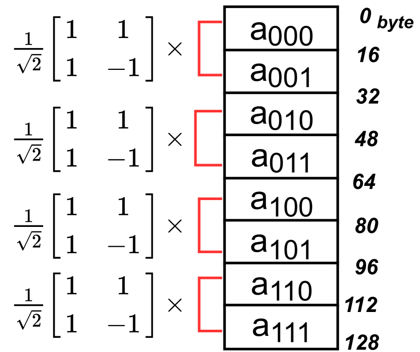
(a) $H$ gate on qubit 0

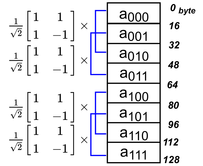
(b) $H$ gate on qubit 1

Figure 1: Applying an $H$ gate on qubits 0 and 1 of a 3-qubit quantum system ($a_{000},a_{001},...a_{111}$, little-endian).

Efficient quantum circuit simulation requires optimizing data locality in performing the matrix multiplication operations. One observation on the computational pattern suggests that this task follows a relatively cache-friendly pattern: a pattern shown in Fig. 1(a) conducts sequential memory accesses (i.e., step size $s=1$); the pattern shown in Fig. 1(b) (i.e., $s=2$) would exhibit a similar cache efficiency as the Fig. 1(a) since a step size of 2 would allow the access to the vector’s elements to remain in the same cache line (typically 64 bytes for modern CPUs). In fact, the step size $s$ for picking up the two elements of the vector is determined by the position $i$ of the target qubit, i.e., $q_{i}$, accessed by the quantum gate can be computed as $s=2^{i}$.

However, as the number of qubits needed by the quantum circuit scales up, the working set size of the simulation task would inevitably exceed the cache size. For a modern CPU usually featuring a L3 cache (e.g., 32MB) shared by all cores, a L2 cache (e.g., 1MB) per core and a L1 cache (e.g.. 64KB) per core, the performance of the circuit simulation on more than 21 qubits (i.e., $2^{21}\!\cdot\!16=32$MB) would be degraded by the capacity cache misses on L3 cache.

III-B Hierarchical Circuit Simulation

To address the above challenge and improve the performance of quantum circuit simulation, HiSVSIM implements the hierarchical simulation framework that executes the input circuit as a sequence of sub-circuits (i.e. parts), each of which contains a portion of the original gates. Therefore, executing the gates inside each part would only occupy a smaller working set size in the memory, which presents a better locality compared to the non-hierarchical scenario.

HiSVSIM makes the following design choices: a) HiSVSIM considers the dynamic execution of the gates in a quantum circuit as a DAG, and converts the circuit partitioning problem into a (acyclic) graph partitioning problem (Section IV); b) HiSVSIM ensures the correctness of the proposed part-based simulation via the novel Gather-Execute-Scatter model (Section III-C); c) HiSVSIM enforces a consistent layout for qubit organization across multiple levels in the hierarchy and remaps the qubits in a part to the lower level simulation.

III-C HiSVSIM Framework Overview

Fig. 2(a) illustrates the overview of HiSVSIM framework. Given a quantum circuit that is comprised of a sequence of gates applied to $n$ qubits, HiSVSIM uses the circuit partition module to parse the circuit and generate several parts/subcircuits of the circuit. Each of the resulting parts of the circuit would impact a smaller number of qubits than the original circuit, enabling the hierarchical simulation that the new instances of the state-vector simulator can be launched over the parts of the circuit. During the simulation, the amplitudes in the corresponding positions of the states with greater strides (i.e., handled by the “outer” state vector simulator) are gathered into the low-level quantum states (i.e., handled by the “inner” state vector simulators), and after the execution of the gates inside that part, the result amplitudes are scattered back to their original positions in the outer state vector for the next round of gather-execute-scatter operations.

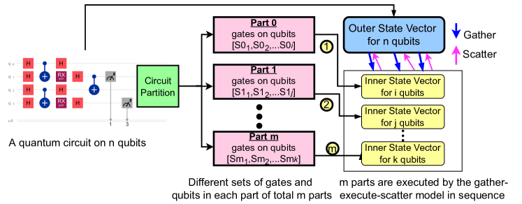
(a) HiSVSIM workflow overview. The input circuit is converted into multiple parts via the partition module, and the resultant parts of the original circuit to create smaller inner state vector instances. For each of them, the gather-execute-scatter model is applied against the outer state vector that is created for the input circuit.

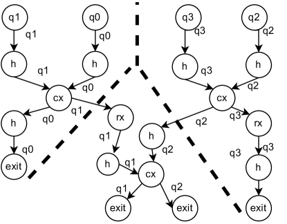
(b) The DAG representation of the example circuit shown in Fig. 2(a). The dotted lines illustrate the desirable partitions of the graph.

Figure 2: The main HiSVSIM workflow to partition the input circuit and perform part-based quantum circuit simulation.

For example, to partition the circuit shown in Fig. 2(a) (Fig. 2(b) depicts the circuit’s DAG), one partition strategy is to divide the circuit into three parts: part 0 (left), part 1 (right) and part 2 (bottom-middle), where each part contains 2 qubits in the working set. This way, both the gate dependencies and the qubit dependencies are preserved. While the simulation still sweeps through the entire “outer” state vector, the actual operation occurs on 4-element state vectors. In general, such cache-resident inner state-vectors can reduce accesses to data that resides in DRAM from the outer state vector, reducing overall memory access costs.

The workload distribution for the algorithm is as follows: First, the DAG is generated and partitioned. Second, the partitioning information is used to decide the computation of parts sequentially (i.e., workload in different parts are not computed in separate processing elements). For a part at hand, a subset of the elements in the original state vector (i.e. outer state vector) is designated, and gathered to “inner state vector”s. These are disjoint and collectively exhaustive over the whole state vector. Within the part, all gates belonging to that part are computed against the inner state vector. After the computation of a part, the results are scattered back to the “outer state vector”. And the distinct state vectors for the next part is loaded into the inner state vector for computation.

Algorithm 1 describes how the quantum states get gathered and scattered between the outer and inner state vectors, using the example circuit shown in Fig. 2(a). To execute the first part (i.e., $p=P_{0}$), an inner state vector in_sv is created based on the qubits residing in $P_{0}$ (i.e., $[S0_{1},S0_{2},...S0_{i}]$ as shown in Fig. 2(a)). Given $S0_{1}=q1$ and $S0_{2}=q0$ , the qubits that do not participate in any gates in $P_{0}$ are $q2$ and $q3$. For all combinations of bit values of $q2$ and $q3$, HiSVSIM moves the data addressed by $[q3,q2,q1,q0]$ from out_sv to the corresponding $[q1,q0]$ positions in in_sv. This process is referred as Gather. The Scatter process sends the states back to out_sv after the execution of the gates through in_sv. On completion of a number of $2^{t}$ Gather-Execute-Scatter processes (assuming t equals to the number of qubits not residing in the current part), out_sv is ready for the next part.

Input :  out_sv = state_vector(num_count),

Partitions = an acyclic partitioning of gates

1 for $p$ in Partitions do

2       Get gate_list from $p$

       w = working set size $\triangleright$ inner qubit count

       in_sv = state_vector(w) $\triangleright$ initialize with size w

       $\triangleright$ e.g., binary permutations of 2 qubits = {(0,0),(0,1),(1,0),(1,1)}

3       for each binary permutation of ($q_{n-1}$, …, $q_{w}$) do

             $\triangleright$ Gather

4             for each binary permutation of ($Sp_{1}$, …, $Sp_{w}$)  do

5                   in_sv[$Sp_{1}$, …, $Sp_{w}$] ←out_sv[$q_{n-1}$, …, $q_{w}$, $Sp_{1}$, …, $Sp_{w}$]

6                  

7            executeSimulation(in_sv, gate_list)

             $\triangleright$ Scatter

8             for each binary permutation of ($Sp_{1}$, $Sp_{w}$)  do

9                   out_sv[$q_{n-1}$, …, $q_{w}$, $Sp_{1}$, …, $Sp_{w}$] ←in_sv[$Sp_{1}$, …, $Sp_{w}$]

10                  

11            

12      

Algorithm 1 The algorithm to execute a circuit given an acyclic partitioning.

III-D Multi-node Design

For circuits that require a large number of qubits, a single compute node will not be able to hold the entire quantum state vector in memory. HiSVSIM extends our hierarchical simulation design to develop a multi-node MPI-based hierarchical simulation for distributed-memory quantum circuit simulations. The first task to achieve this is to distribute the quantum states from the state vector across all MPI ranks to ensure that each MPI rank can execute all the gates inside a part locally. Since different parts may contain different qubits, to switch between parts, each MPI rank needs to gather the states residing in the remote MPI ranks to form new local states, which triggers a global communication across MPI ranks.

Specifically, assuming an $n$-qubit quantum system, HiSVSIM identifies the qubits as two sets: the number of $p$ process (or MPI rank) qubits and the number of $l$ local qubits, where $n=p+l$. Note that this design requires the number of MPI ranks to be a power of two. For example, a 4-qubit quantum state vector simulated by 4 MPI ranks (i.e., $p=2$ and $l=2$) would be addressed as $[a_{3},a_{2},|\ a_{1},a_{0}]$. The 4 MPI ranks are addressed by the most significant bits $(a_{3},a_{2})$, with the local quantum state elements of each MPI rank addressed by $(a_{1},a_{0})$. Fig. 3(a) illustrates the MPI-based layout of the quantum states for the scenario when part $P_{0}$ of the example circuit (shown in Fig. 2(a)) is executed by HiSVSIM. After $P_{0}$ has been executed, HiSVSIM uses the new local and process qubits designated for the next part to determine the state to be gathered for each MPI rank. The examples shown in Fig. 3(b) and Fig. 3(c) illustrate the MPI messages received by rank 0 and rank 1, respectively, and the amplitude values and locations in the send/receive buffers after $P_{0}$. Fig. 3(d) shows the final amplitude distribution across all MPI ranks for the new part ($P_{1}$) to be executed, where the process qubits are $(a_{1},a_{0})$ and the local qubits are $(a_{3},a_{2})$.

Our MPI-based implementation to distribute and gather qubits in the multi-node scenarios offers a general interface for other simulators to use as a library.

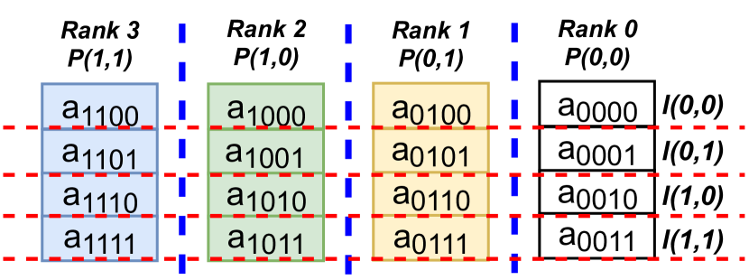
(a) The initial state distribution across 4 MPI ranks.

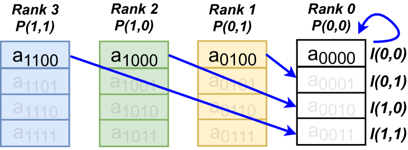
(b) Example: the data gathered by rank 0 switching from Part 0 to Part 1.

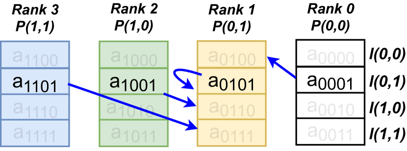
(c) Example: the data gathered rank 1 switching from Part 0 to Part 1.

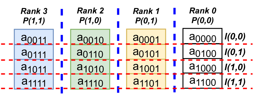
(d) Final distribution of the state vector amplitudes after across-rank communication.

Figure 3: The examples of MPI messages across MPI ranks to gather and update local state vector of rank 0 and 1.

IV Quantum Circuit Partitioning

The memory requirement for a given number of qubits is exponential and each iteration of the simulation starts and ends with memory read/writes between the inner and outer state vectors (Alg. 1). Thus, an intuitive partitioning approach would be to minimize the number of parts, i.e., minimizing the number of bulk read/writes (or MPI communications) of this exponential amount of data. Hence, the objective of the partitioning is to create the smallest number of parts while keeping the number of qubits of each part under a limit. If there are cyclic dependencies between parts (i.e., parts require computation of gates from each other), then it would require multiple data transfers to synchronize. Therefore, having cyclic dependencies makes it hard to count and minimize the number of bulk read/writes and MPI communications. Thus, a circuit should be partitioned in a way that allows each part to be loaded into the inner state vectors for computation only once after all of its dependencies are met, i.e., an acyclic manner with a topological order. And, finding such a partition should be fast and efficient to potentially bring runtime improvement.

IV-A Model

We consider a directed acyclic graph (DAG) $G=(V,E)$, where the vertices in set $V=\{v_{1},\ldots,v_{n}\}$ represent computational gates, and edges represent the qubits needed for the computational gates. Given $v_{i}\in V$, $pred_{i}=\{v_{j}\;|\;(v_{j},v_{i})\in E\}$ is the set of predecessors of gate $v_{i}$ in the graph, and $succ_{i}=\{v_{j}\;|\;(v_{i},v_{j})\in E\}$ is the set of successors of gate $v_{i}$. We create artificial computational gates for initialization and destruction of the qubits, i.e., for each qubit, there is an entry and an exit gate that does not represent any computation. Entry gates have no predecessor and one successor that is the first computational gate the corresponding qubit enters. And, exit gates have no successors and one predecessor.

For each computational gate, the total incoming edge weight is equal to the outgoing edge weight, which is the number of qubits involved in the computation of this gate. No qubit is input to multiple gates at the same time. Thus, it is possible to trace each qubit through the edges between gate vertices. The gates are naturally in a topological execution order where they can be executed only after all of their predecessors are executed, i.e., the edges represent the qubit dependency between the gates.

The Circuit Partition (Fig. 2(a)) accepts a DAG representation of the circuit, and a maximum working set size $L_{m}$ that is common for all parts as input. It solves the acyclic $k$-way partitioning problem $P=\{V_{1},\ldots,V_{k}\}$ of the DAG $G=(V,E)$: the set of vertices $V$ is divided into $k$ nonempty, pairwise disjoint, and collectively exhaustive parts satisfying three conditions: i) The working set size of individual parts do not exceed $L_{m}$. ii) The partition is acyclic. There is a path between $V_{i}$ and $V_{j}$ ($V_{i}\leadsto V_{j}$) if and only if there is a path between a vertex $v_{i}\in V_{i}$ and a vertex $v_{j}\in V_{j}$. The acyclic condition means that given any two parts $V_{i}$ and $V_{j}$, we cannot have $V_{i}\leadsto V_{j}$ $and$ $V_{j}\leadsto V_{i}$. A part-graph of $G$ is a graph where the nodes represent the parts in $G$ (i.e., all nodes in the same part are contracted to a single node) and the edges represent the cumulative edges between parts of $G$. iii) The number of parts $k$ is minimized. Similar to the graph partitioning problem, the acyclic DAG partitioning is an NP-Hard problem and there is no k-approximation for $k>2$ [20]. Thus, all feasible algorithms that solve this problem are heuristics. The output of partitioning is a part assignment for each node (gate). After partitioning, gates are collected according to their parts and executed with respect to the original order among those in the same part.

The working set size, $L(V_{i})$ of a part $i$, is the number of qubits needed for all gates in that part. That is, if gate $A$ needs $q0$ and $q1$ and gate $B$ needs $q0$ and $q2$, these two gates require 3 qubits in total. If $V_{i}=\{A,B\}$, then $L(V_{i})$ = 3. We can imagine edges having labels in the computational gate graph. Each entry qubit emits an edge with the label of qubit they are initializing, and each gate these qubits participate in, they are represented by a single in-edge and a single out-edge. Since a qubit cannot be passed to two different gates at the same time (i.e., gates have a time order), the incoming edges of a gate/part are always unique.

IV-B Proposed Partitioning Methods

We propose three partitioning approaches:

IV-B1 Natural Topological Order Cutoff (Nat)

Nat follows the execution order of the gates in the original circuit, and computes the working set size. When the working set size exceeds the limit $L_{m}$, the gates before the limit is exceeded are assigned as one part. Then, working set size is reset and this process is repeated for the remaining gates. Natural ordering is deterministic and falls short when the order contains alternating operations for larger number of qubits than $L_{m}$.

IV-B2 DFS Topological Order Cutoff (DFS)

DFS remedies this problem by testing several random DFS topological orders of the gates instead of the deterministic natural topological order, and picks the one that yields the smallest number of parts. The part assignment follows the same procedure.

IV-B3 Acylic-partitioning-based Partitioning (dagP)

We propose a novel acyclic DAG-partitioning-based heuristic by extending and modifying a recent open-source, state-of-the-art acyclic DAG partitioner [20, 21]. It presents an acyclic DAG partitioning algorithm that consists of an acyclic agglomerative clustering, recursive-bisection-based initial partitioning, and refinement phases. Given a DAG and $k$, their algorithm recursively divides the DAG, until the desired $k$ is achieved, while minimizing the edge cut (total weight of edges that connect nodes from different parts) as the objective. Using a black-box partitioner for our problem definition is not trivial. There are major changes to the partitioning objective, criteria, and greedy approaches as well as some minor changes in order to preserve/improve the performance of a partitioner. Without these modifications, the partitioners may not ever find a valid partitioning abiding the required constraints. We replaced the edge cut objective with minimizing the number of parts, while ensuring each part’s working set size is under given limit. We modified related computations in all phases of the partitioning. We added a final merging phase that is not present in the original algorithm. We used the authors’ suggested parameter values except for the imbalance ratio (i.e., $\epsilon\leq 1.5$) since the weight balance of the parts is not critical. We refer the readers to the corresponding article for further details on the original algorithm and only briefly discuss our major modifications.

The original algorithm requires the final number of parts, $k$, as an input parameter. Our problem requires the algorithm to discover the necessary (minimum) number of parts. Our algorithm starts by computing the working set size of the graph $L(G)$ (it is the total number of qubits, i.e., number of $entry$ nodes). If it is greater than $L_{m}$, the graph is partitioned into two roughly balanced subgraphs (in terms of the number of nodes). The recursive bisection operation dives into the subgraphs and partitions them until each one’s working set size is less than or equal to $L_{m}$. If the working set size of a subgraph is less than or equal to $L_{m}$, then the partitioner stops and returns. At the end of recursive bisection, we run a merge phase in which a clustering algorithm is applied on the global view of the graph via the part-graph to merge existing parts until there is no more possible valid mergers, i.e., the merger does not create cycles in the part-graph and does not violate the $L\leq L_{m}$ criterion.

The runtime performance of the partitioner significantly depends on how efficiently one can compute updates when a vertex is moved from one part to another. The edge cut, objective of the former problem [20, 22], can be efficiently updated. Our dagP algorithm takes advantage of the following information to compute working set size at each phase efficiently. Since the computational gate graph of quantum circuit simulation has the property where the number of inputs of a gate is equal to that of outputs and all of them represent unique qubits, one only needs to count the in-edges to a part, and the number of $entry$ nodes within the part.

One question that may arise is whether the circuits with higher number of entanglements with many qubits complicates the partitioning. The partitioner considers the circuits as DAGs where the edges contain all dependency information and HiSVSIM makes no assumptions on the properties of the circuits. Larger entanglements are just nodes with higher degrees. This may deteriorate the performance for the greedy localized approaches such as Nat and DFS for finding the best valid partitions. The goal of dagP approach is to find the best partitioning using a global view of the computation DAG, which overcomes this deficiency of the former two approaches.

Both Nat and DFS methods have a localized view of the gates at hand whereas dagP benefits from a broader view of the whole circuit graph. Compared to the runtime of the quantum circuits, all three have negligible computation times (up to milliseconds).

Figure 4 shows a toy example for partitioning with Nat and dagP approaches, respectively. Top-left and top-right subgraphs show the respective part-graphs. DFS approach can return any number of parts between these two examples depending on the random DFS topological orders at hand.

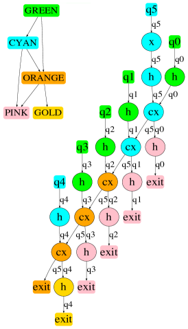
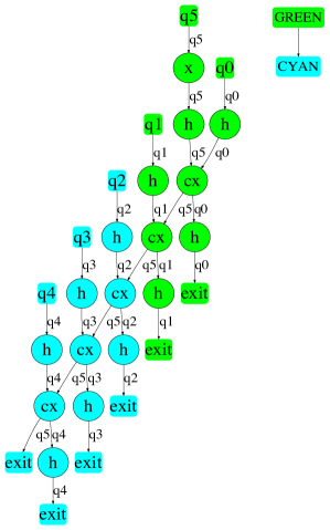
Figure 4: A toy example partititoning of bv graph with 6 qubits with qubit limit 4 using Nat (left) and dagP approach (right).

Multi-level partitioning. The acyclic DAG partitioning with recursive bisection presents an opportunity to prepare partitions for varying $L_{m}$’s at different scales, and thus, can be better exploited for the multi-node design (Sec. III-D), i.e., inter-node data distribution and intra-node cache locality optimization. The partitioning is run on the original circuit graph with the first-level limit to break it down into a number of parts, then, each one is recursively partitioned further using the second-level limit.

The $L_{m}$’s are decided with the system configuration in mind. The first-level partitioning uses a $L_{m}=l$ for the local state vector (Sec. III-D), while the second-level partitioning uses a size that keeps the size of the second-level inner state vector under the LLC cache size. When the number of qubits in a part is less than $L_{m}$, we add the qubits from the higher level part to exploit spatial locality.

V Experimental Evaluation

Table I lists the 13 benchmark quantum circuits, from QASMBench suite [23], used in this paper. Circuits cover a variety of application domains that represent the essential areas in quantum computing. Note that we explore two sets of qubit and gate configurations for the bv, cc, and ising circuits to investigate how much more efficiency our HiSVSIM could bring to the same quantum algorithms in different scales.

We ran our experiments on a workstation (Intel Cascade Lake, 448 CPU cores, 8 sockets, 8 NUMA nodes, 6TB memory) and the Frontera [24] supercomputing cluster at TACC (each node in the cluster features dual Intel Xeon Platinum 8280 with 2.7GHz clock rate, 56 cores, 192GB DRAM and the InfiniBand HDR-100 network). For each circuit, we examine the performance of the simulation with three partitioning strategies (Nat, DFS, and dagP) and compare the results with the baseline simulation results using Intel’s IQS [10]. We translate the OpenQASM gates into IQS gates to ensure that HiSVSIM and IQS execute identical circuits.

V-A Single node experiments

On the single machine scenario, we configure the HiSVSIM with varying number of OpenMP threads (i.e., 2,4,8,16,32,64,128), and HiSVSIM exhibits a close-to-linear speedup in this strong scaling case. Table II shows the breakdown of the memory usage (profiled with vTune Profiler [25]) with a single thread for each partitioning strategy to indicate why dagP offers the most efficient simulation. Among three strategies, dagP always leads to the lowest DRAM stalled time, which reflects the more efficient cache access pattern. For the example circuits presented in Table II, 35.7% and 20.2% of pipeline slots are for memory loads and stores in Nat partitioning on bv and ising respectively, which far outweighs the DFS and dagP. In particular, DFS and dagP on ising produce similarly partitioned circuits, hence the memory access patterns are comparable. Similar trends can be observed in all circuits but qpe (where Nat outperforms DFS and dagP). For brevity, we omit the rest of the results.

To evaluate the quality of the dagP heuristic, we implemented an integer linear programming (ILP)-based optimal solution to our modified acyclic DAG partitioning problem. The ILP solution takes minutes for even the smaller circuits compared to the microseconds of the dagP heuristic since the problem is NP-Hard and ILP formulation gets exponentially more complex. Out of 52 combinations (13 inputs, 4 qubit limits), dagP finds the optimal number of parts for 48 cases and only differs by 1 or 2 for the rest.

TABLE I: Benchmark description.

Circuit	Description	qubits	gates	Mem.
cat_state [26]	Coherent superposition	30	60	16 GB
bv [27]	Bernstein-Vazirani algorithm	30	102	16 GB
qaoa [4]	Quantum approx. optimization	30	1,380	16 GB
cc [28]	Counterfeit coin finding	30	149	16 GB
ising [29]	Quantum simulation for ising model	30	354	16 GB
qft [23]	Quantum Fourier transform	30	2,235	16 GB
qnn [23]	Quantum neural network	31	164	32 GB
grover [30]	Grover’s algorithm	31	207	32 GB
qpe [31]	Quantum phase estimation	31	5,731	32 GB
bv35 [27]	Bernstein-Vazirani algorithm	35	119	512 GB
ising35 [29]	Quantum simulation for ising model	35	414	512 GB
cc36 [28]	Counterfeit coin finding	36	106	1 TB
adder37 [32]	Quantum Ripple-Carry adder	37	154	2 TB

TABLE II: Memory access breakdown.

Circuit	Strategy	% of clockticks				(%)Memory/ Pipeline slots	Execution time (s)
		L1	L2	L3	DRAM
	Nat	6.1	4.0	4.4	19.8	35.7	209.7
bv	DFS	2.3	3.1	3.8	16.6	26.1	172.8
	dagP	2.9	6.5	2.0	4.3	20.9	163.2
	Nat	7.0	2.7	4.4	11.2	20.2	613.5
ising	DFS	1.5	1.2	1.9	5.8	6.6	455.6
	dagP	1.3	1.2	2.1	5.5	7.5	454.1

V-B Multiple node experiments against IQS

In this section, we increase the number of nodes from 16 to 256, on Frontera system. The circuits are configured as two groups: one MPI rank runs on each node for circuits that have less than 32 qubits, and 2 and 4 MPI ranks on a node (i.e., 512 and 1024 MPI ranks on 256 nodes in total) for circuits with 35-37 qubits. (MPI ranks are also referred as Cores in the figures). Figure 5 shows the simulation performance of HiSVSIM compared to IQS for each circuit. The comparison results are presented as the improvement factor (referred as factor below) normalized over the simulation performance of IQS using the same resources. Any value above 1 means the specific approach improves the total runtime over IQS.

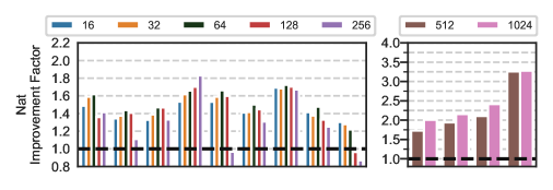
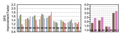
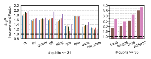
Figure 5: The improvement factor over Intel IQS of our partition strategies for different MPI ranks.

Overall, HiSVSIM outperforms the IQS for all the circuits via dagP strategy on various numbers of MPI ranks, where the improvement factor for the maximum end-to-end execution time ranges from $1.15\times$ (qpe on 128 MPI ranks) to $3.87\times$ (adder on 1024 MPI ranks), with a geometric mean of $1.7\times$ across all the MPI rank configurations. The right subfigures in Fig. 5 show circuits with larger number of qubits, evaluated on 512 and 1024 cores. As the number of qubits and the computational resources increase, our algorithms scale better compared to IQS baseline. bv, ising, and cc graphs with 30 qubits have improvement factors up to $1.7\times$, $1.9\times$, and $2\times$ whereas bv35 has up to $2.7\times$, ising35 has up to $2.5\times$, and cc36 has up to $3.2\times$. This demonstrates the benefit of introducing circuit partitioning and hierarchical simulation.

Comparing across three partitioning strategies, dagP consistently results in fastest simulation time for all the circuits but qpe. Take the 256 MPI ranks cases for example, the dagP offers 29% and 30% higher improvement factors over Nat and DFS on average. In addition, at the 128 and 256 MPI ranks configurations, the improvement factors obtained with Nat and DFS partitioning show a decreasing trend (7 of 10 circuits) compared to their 32 and 64 ranks configurations, while dagP exhibits the opposite trend indicating that dagP partitioning provides a consistent improvement over the baseline simulator.

In summary, dagP partitioning offers a mean of 2.1 improvement over the baseline IQS simulation results across all 13 circuits when largest number of MPI ranks applied (i.e. 256 and 1024 for the corresponding circuits). We demonstrate that the simulation for the circuits with a larger number of qubits ($\geq 35$) have more prominent improvement factors (from $2.5\times$ to $3.9\times$ with the average $3.0\times$). This shows the effectiveness of dagP partitioning approach over the baseline and the other two partitioning strategies.

V-C Strong scaling

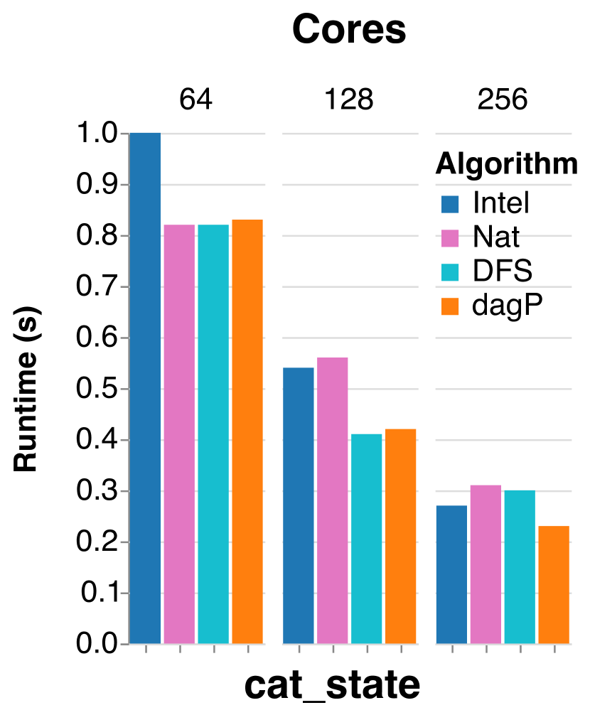
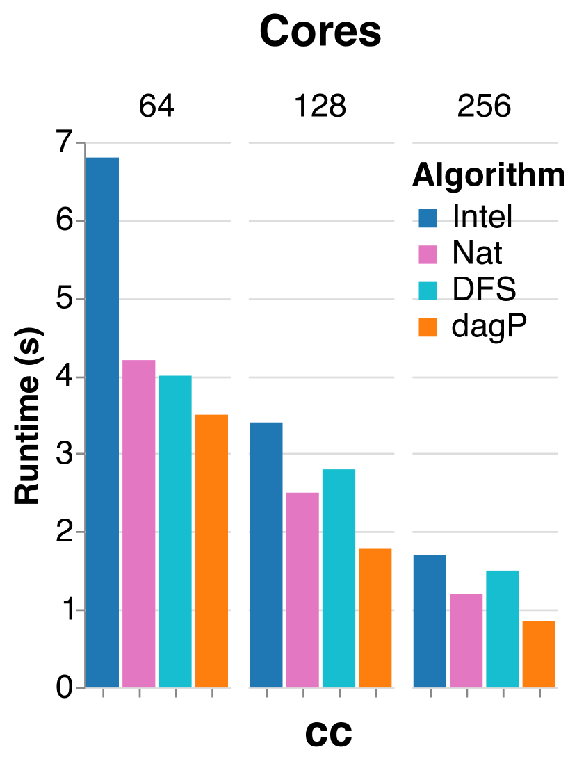
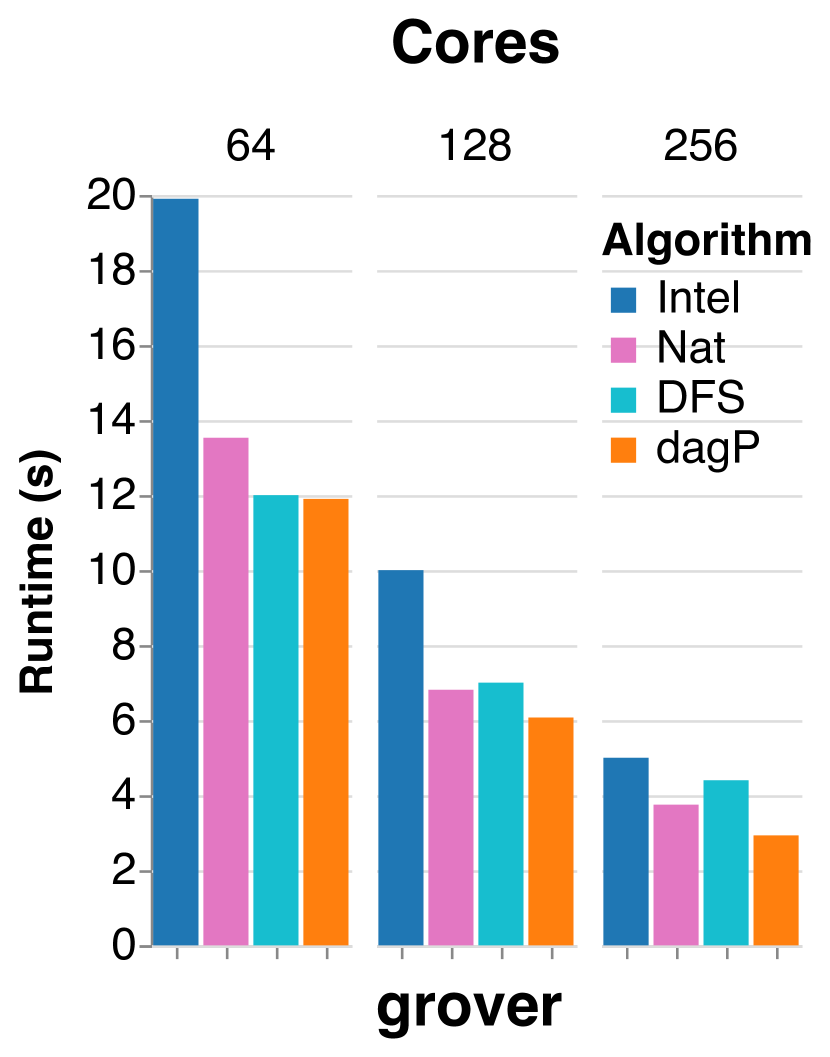
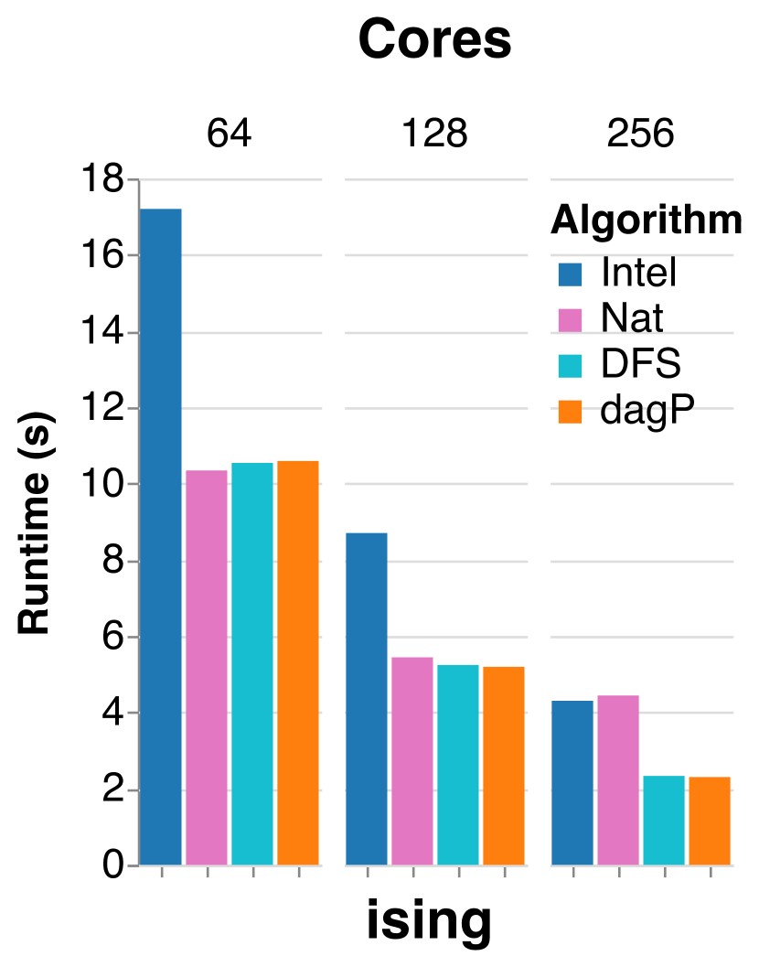
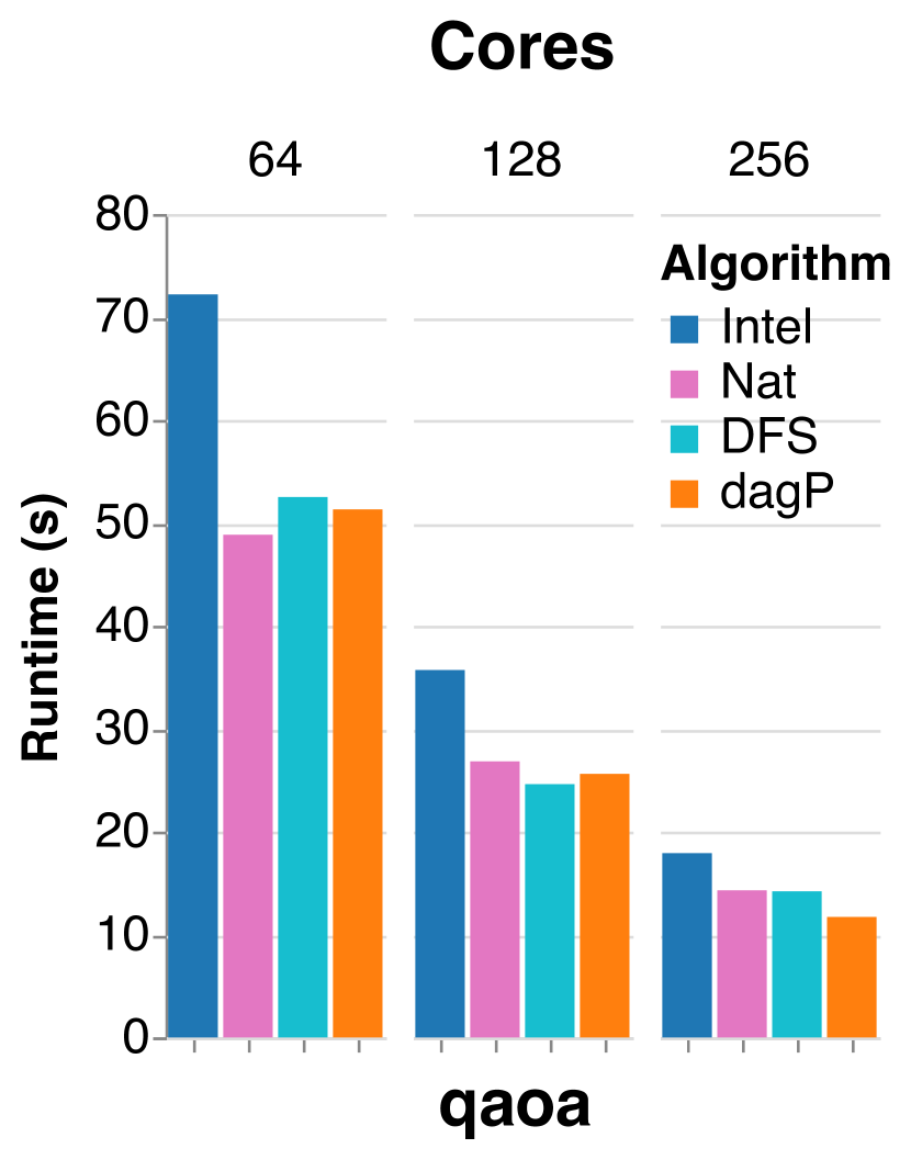
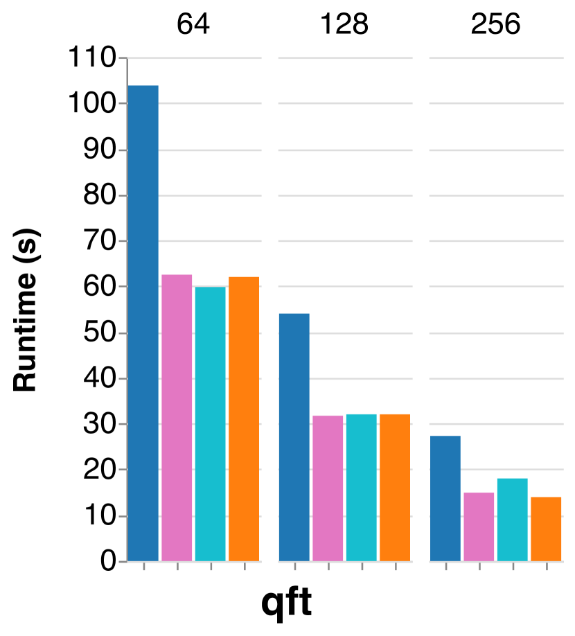
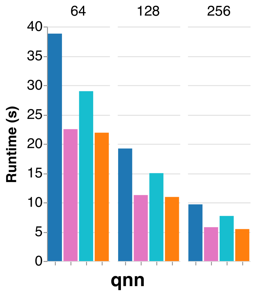
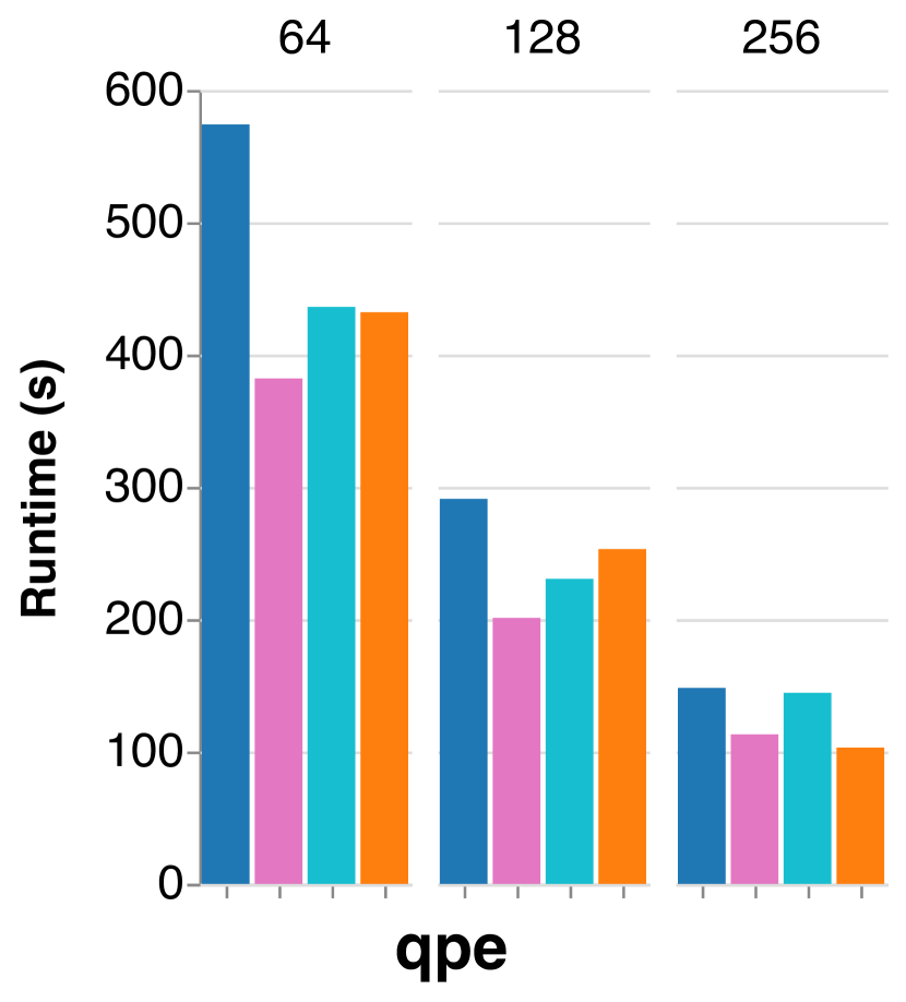
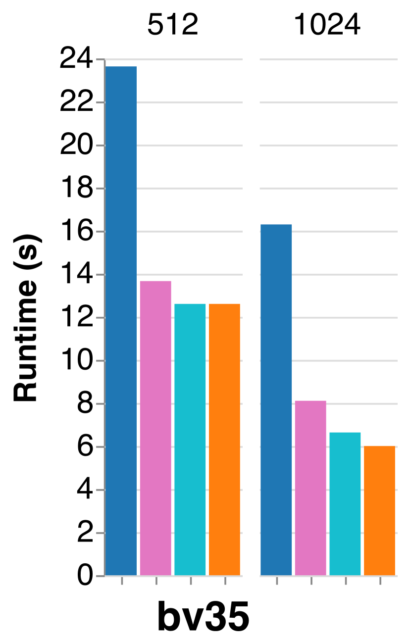
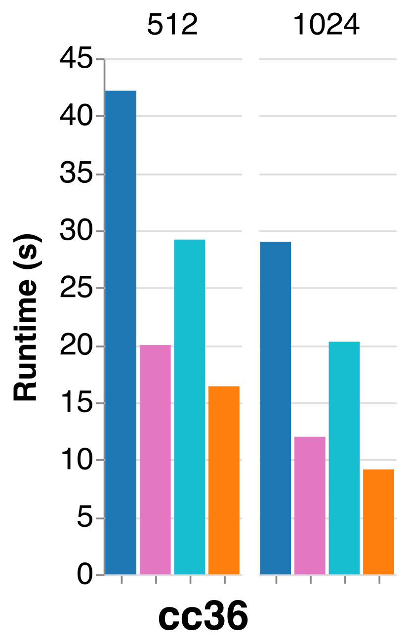
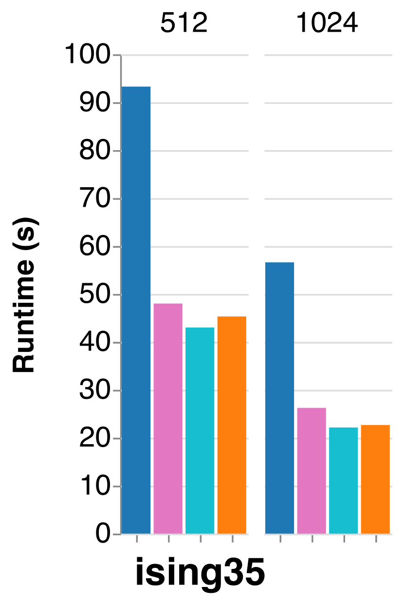
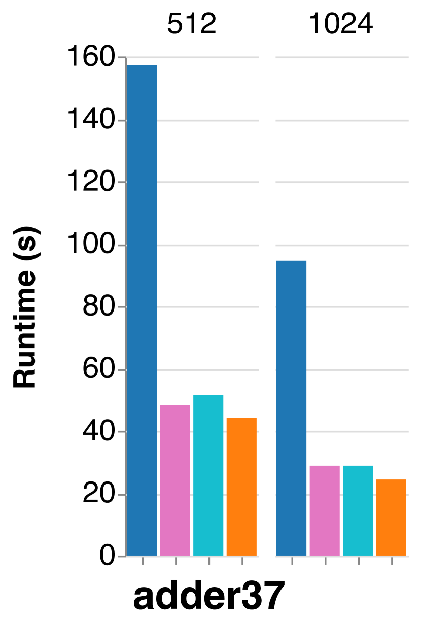
Figure 6: Runtime of the input circuits.

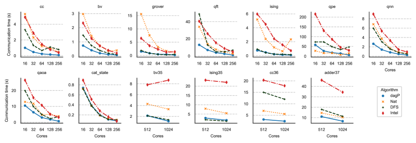
Figure 7: Average communication time of the three partitioning variants of HiSVSIM and IQS for all input circuits.

In the strong scaling case, Fig. 6 shows the maximum end-to-end simulation time for each circuit partitioned with Nat, DFS, and dagP strategies and the IQS for varying number of MPI ranks. (Due to the limited space, we omit the results for 16 and 32 MPI ranks while the trend is consistent). Since HiSVSIM allows computation and communication overlapping, i.e. each rank can continue computation as long as it receives data from other ranks), we report the average MPI communication time across all the ranks per circuit for HiSVSIM. We leverage remora [33] to obtain the timing details for the computation and MPI calls of IQS. The minimal overhead of profiling with remora is remedied by applying the communication/computation ratio to the end-to-end execution time obtained without remora present.

We make the following observations: (I) HiSVSIM shows a close-to-linear speedup for all the partitioning strategies; (II) For HiSVSIM, both the average computation and communication ratios of the simulation times show the overall close-to-linear scaling effect across all the configuration cases and circuits; (III) HiSVSIM consistently offers a faster simulation in the computation portion than the IQS across all circuits. Note that with HiSVSIM, the average computation time is observed similar across different partition strategies.

MPI communication benefit demonstration. Fig. 7 shows the per-circuit average communication time for the three strategies and IQS, and Fig. 8 provides an overall summary. As seen in the figures, dagP achieves the fastest communication time across all the cases, and IQS spends relatively longer communication time for all the circuits, especially for the circuits that contain a larger qubit count. Fig. 8 shows that dagP leads to the lowest geometric mean of the average communication ratio compared to Nat, DFS and IQS cases for all number of cores tested, and the DFS outperforms the IQS except for 256 MPI ranks. The trend of the lines through increasing number of cores show that dagP has the best scaling of average communication ratio as well.

Next, for an overall comparison of our algorithm variations, we use performance profiles. A performance profile shows the ratio ($\rho$) of all input instances where an algorithm performed within a factor ($\theta$) of the best performing algorithm [34]. Here, an instance is a unique test case, e.g., a pair of an input and a number of cores used. Figures 9(a) and 9(b) show performance profiles of the three partitioning approaches and IQS baseline for the total runtime and average communication time, respectively. For instance, in Fig. 9(a), dagP performs the best 65% of the time while DFS and Nat perform the best approximately 18% and 25% of the time. It also shows dagP performs within $1.3\times$ the best total runtime for all instances. In addition, we see that the best result for the IQS is only at $1.2\times$ the best total runtime. Similarly, in Fig. 9(b), we see that dagP has the lowest communication time for 75% of the input instances. And, for roughly 40% of the instances, the other two variants cannot reach an average communication time that is even within $2.0\times$ the communication time of dagP approach.

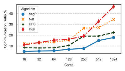
Figure 8: Geometric mean of average communication ratio of the three partitioning variants and IQS for all circuits.

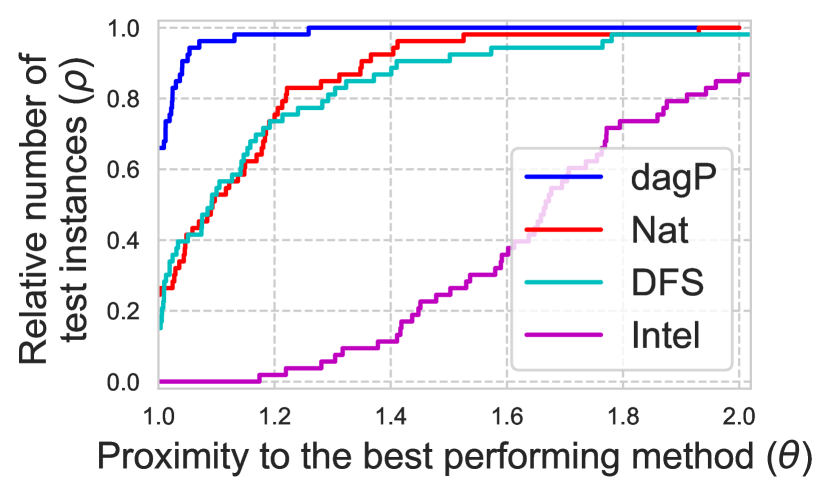
(a) total runtime

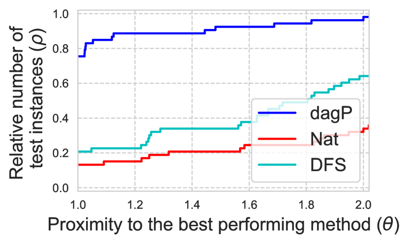
(b) avg. communication time

Figure 9: Performance profile of time metrics comparison for IQS and three HiSVSIM partitioning methods.

V-D Multi-level partitioning

Finally, we demonstrate the efficiency gained via exploiting multi-level memory hierarchy in the multi-node system: The first level partition that uses the main memory of a node to hold the local state vector and communicates with other nodes to update the local state vector after finishing a part, and a second level partition that further partitions the qubits contributing to the local state vector into new parts, and executes the gates of each new part to improve cache locality.

In some circuits a natural, intuitive partitioning of the gates contains less unique qubits than the limits for first-level and second-level partitioning in each part. In this case, the second-level partitioning returns the identical part to the first-level part at hand. Thus, we evaluate the multi-level partitioning on the circuits that contain different sets of parts. For all circuits that are not shown in the figure, the single- and multi-level HiSVSIM uses the identical partitioning.

Figure 10 shows the execution times of HiSVSIM for the single-level (i.e., the results shown in Fig. 6) and multi-level partition with the 256 MPI ranks for qaoa, qft, qnn, and qpe and 1024 MPI ranks for adder. While the single-level partition results collected represent the most advanced cases by far, the multi-level partition strategy offers a further improvement over the prior “best” cases except for qnn which is 0.1s slower. The simulation time goes from 24.4s to 16.7s (adder), 14s to 12.7s (qft), 11.8s to 11.3s (qaoa) and 103s to 84s (qpe), with the average of 15.8% reduction. This translates to up to $5.67\times$ improvement over IQS, and $1.47\times$ over our best single level variant.

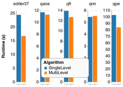
Figure 10: Runtime for the single-level with the best performance and the multi-level.

VI GPU Extrapolation

As mentioned earlier, our acyclic graph partitioning enables the optimization space to balance between the local computation and remote communication. To demonstrate the possible use of our approach with other simulators, we take the state-of-the-art GPU-based quantum circuit simulator - HyQuas [18] and present a hybrid approach: using HiSVSIM for circuit partitioning and communication and using HyQuas kernel for the computation on GPUs and compare it with the simulation time of using HyQuas on multi-GPU nodes.

We use 4 GPU nodes in our cluster to run the qaoa_28 circuit (taken from the HyQuas repo) with HyQuas. Each node has an NVIDIA V100-PCIE-16GB GPU. Nodes connect via the InfiniBand hardware. We take the following steps to ensure that the computation to be conducted on GPUs carries the same amount of work as computed by HiSVSIM: (i) We partition the qaoa_28 circuit into two parts and remap the qubits in each part to model the reordering inside the local state vector. This step ensures the global qubit index is converted to the local slot index. (ii) After remapping, we modify the total qubit number in each part file to fit in the computation model of HiSVSIM. For example, in four nodes case, to execute a 28 qubit circuit, HiSVSIM organizes the total qubits as 26 local qubits and 2 MPI process qubits (as described in Sec III-D, $log(4)=2$). Each part of the original circuit needs to meet the 26 qubits requirement; (iii) we execute the gathered sections of parts (inner state vector) with single-GPU HyQuas on each node. We replace the local computation component of HiSVSIM (with HyQuas on inner state vector) and leave the rest of HiSVSIM unchanged. This way, the cross-node data redistribution stays the same. Since the whole quantum state fits in the memory of available GPUs, there is no additional CPU/GPU communication.

The original qaoa_28 circuit is partitioned with dagP, DFS and Nat as shown in Table III. Different strategies generate different number of parts. The total number of gates matches with the original qaoa_28 circuit in the HyQuas paper. Table III shows the execution time of each part executed with single-GPU HyQuas on one V100 GPU per node. One can observe that the total execution time on GPU for different strategies is close to each other, which is similar to the HiSVSIM multi-node CPU cases.

Table IV shows the end-to-end performance estimate on this hybrid approach - using HiSVSIM for partitioning and communication and HyQuas for computation. The result shows that the hybrid approach with dagP outperforms original HyQuas, indicating that the acyclic partitioning could accelerate data communication for a highly-optimized GPU-based simulator like HyQuas. Also, among the three strategies, dagP outperforms Nat and DFS, which shows promise for future HiSVSIM-dagP GPU implementation.

TABLE III: QAOA Partitioning breakdown and runtimes on GPUs. qubits: the number of qubits in each part.

Strategy	parts		qubits	gates	total gates	time (ms)	total (ms)
dagP	2	$P_{0}$	22	747	= 1652	146.1	329.8
		$P_{1}$	24	905		183.7
DFS	3	$P_{0}$	24	536	= 1652	110.8	337.7
		$P_{1}$	24	637		129.7
		$P_{2}$	20	479		97.1
Nat	6	$P_{0}$	24	24	= 1652	11.9	365.9
		$P_{1}$	24	474		97.7
		$P_{2}$	24	260		64.3
		$P_{3}$	24	305		65.9
		$P_{4}$	24	307		65.8
		$P_{5}$	17	282		60.1

TABLE IV: Estimated QAOA circuit simulation times combining HiSVSIM and HyQuas.

Strategy	Communication (s)	Computation (s)	Total time (s)
dagP	0.5	0.33	0.83
DFS	1.0	0.34	1.34
Nat	2.4	0.37	2.77
HyQuas [18]	-	-	1.47

VII Conclusion

We present a novel multi-level, distributed hierarchical state vector simulator HiSVSIM that employs the graph partitioning algorithms for efficient circuit simulation. The graph partitioning algorithm includes the acyclic-partitioning-based computation ordering approach. We evaluate the efficiency of HiSVSIM with various well-known and representative quantum circuits on Frontera supercomputer with up to 256 nodes and 1024 cores and GPU computation with Nvidia V100. The results show that HiSVSIM, both multi-level and single-level, scales well and achieves a significant improvement over the state-of-the-art open-source distributed quantum circuit simulation systems. The proposed graph-based approach can be useful for other accelerator-based (i.e., GPUs) quantum simulators and real quantum computing platforms.

References

- [1] IBM, “IBM unveils breakthrough 127-qubit quantum processor,” 11 2021. [Online]. Available: https://research.ibm.com/blog/127-qubit-quantum-processor-eagle
- [2] A. M. Dalzell, A. W. Harrow, D. E. Koh, and R. L. La Placa, “How many qubits are needed for quantum computational supremacy?” Quantum, vol. 4, p. 264, May 2020.
- [3] S. Dan and B. M. J., “Temporally unstructured quantum computation,” Royal Society, 2009.
- [4] E. Farhi, J. Goldstone, and S. Gutmann, “A quantum approximate optimization algorithm,” ArXiv, Tech. Rep. arXiv:1411.4028, 2014.
- [5] S. Aaronson and A. Arkhipov, “The computational complexity of linear optics,” in Proc. STOC. ACM, 2011, p. 333–342.
- [6] M. Roetteler, M. Naehrig, K. M. Svore, and K. Lauter, “Quantum resource estimates for computing elliptic curve discrete logarithms,” in Advances in Cryptology – ASIACRYPT. Springer, 2017, pp. 241–270.
- [7] W. Tang, T. Tomesh, M. Suchara, J. Larson, and M. Martonosi, “Cutqc: using small quantum computers for large quantum circuit evaluations,” in Proc. ASPLOS. ACM, 2021, pp. 473–486.
- [8] J. M. Baker, C. Duckering, A. Hoover, and F. T. Chong, “Time-sliced quantum circuit partitioning for modular architectures,” in Proceedings of the 17th ACM International Conference on Computing Frontiers, 2020, pp. 98–107.
- [9] M. Smelyanskiy, N. P. D. Sawaya, and A. Aspuru-Guzik, “qHiPSTER: The quantum high performance software testing environment,” 2016.
- [10] G. G. Guerreschi, J. Hogaboam, F. Baruffa, and N. P. D. Sawaya, “Intel quantum simulator: a cloud-ready high-performance simulator of quantum circuits,” Quantum Science and Technology, 2020.
- [11] N. Khammassi, I. Ashraf, X. Fu, C. Almudever, and K. Bertels, “Qx: A high-performance quantum computer simulation platform,” in Proc. DATE, 2017, pp. 464–469.
- [12] X.-C. Wu, S. Di, E. M. Dasgupta, F. Cappello, H. Finkel, Y. Alexeev, and F. T. Chong, “Full-state quantum circuit simulation by using data compression,” in Prof. of SC’19, 2019, pp. 1–24.
- [13] T. Jones, A. Brown, I. Bush, and S. C. Benjamin, “QuEST and High Performance Simulation of Quantum Computers,” Scientific Reports, vol. 9, no. 1, p. 10736, 2019.
- [14] J. Doi and H. Horii, “Cache blocking technique to large scale quantum computing simulation on supercomputers,” in IEEE International Conference on Quantum Computing and Engineering, 2020, pp. 212–222.
- [15] T. Häner and D. S. Steiger, “0.5 petabyte simulation of a 45-qubit quantum circuit,” in Proceedings of SC ’17, 2017.
- [16] NVIDIA, “Nvidia sets world record for quantum computing simulation with cuquantum running on dgx superpod,” 9 2021. [Online]. Available: https://blogs.nvidia.com/blog/2021/11/09/cuquantum-world-record/
- [17] A. Li, B. Fang, C. Granade, G. Prawiroatmodjo, B. Heim, M. Roetteler, and S. Krishnamoorthy, “Sv-sim: Scalable pgas-based state vector simulation of quantum circuits,” in Proc. SC’21, 2021.
- [18] C. Zhang, Z. Song, H. Wang, K. Rong, and J. Zhai, “Hyquas: hybrid partitioner based quantum circuit simulation system on gpu,” in Proceedings of the ACM ICS, 2021, pp. 443–454.
- [19] S. Williams, A. Waterman, and D. Patterson, “Roofline: An insightful visual performance model for multicore architectures,” Commun. ACM, vol. 52, no. 4, p. 65–76, Apr. 2009.
- [20] J. Herrmann, M. Y. Özkaya, B. Uçar, K. Kaya, and U. V. Çatalyürek, “Multilevel algorithms for acyclic partitioning of directed acyclic graphs,” SIAM Journal on Scientific Computing (SISC), 2019.
- [21] M. Y. Özkaya, A. Benoit, and U. V. Çatalyürek, “Improving locality-aware scheduling with acyclic directed graph partitioning,” in Proc. of the 13th International Conf. on Parallel Processing and Applied Mathematics (PPAM). Springer, Sep 2019, pp. 211–223.
- [22] M. Y. Özkaya, A. Benoit, B. Uçar, J. Herrmann, and U. V. Çatalyürek, “A scalable clustering-based task scheduler for homogeneous processors using dag partitioning,” in 2019 IEEE International Parallel and Distributed Processing Symposium (IPDPS). IEEE, 2019, pp. 155–165.
- [23] A. Li and S. Krishnamoorthy, “QASMBench: A low-level QASM benchmark suite for NISQ evaluation and simulation,” arXiv:2005.13018, 2020.
- [24] D. Stanzione, J. West, R. T. Evans, T. Minyard, O. Ghattas, and D. K. Panda, “Frontera: The evolution of leadership computing at the national science foundation,” in PEARC, 2020, p. 106–111.
- [25] Intel, “Intel VTune Profiler,” https://www.intel.com/content/www/us/en/developer/tools/oneapi/vtune-profiler.html, 2020, online.
- [26] J. R. Gribbin, In search of Schrodinger’s cat : the startling world of quantum physics explained. Wildwood House London, 1984.
- [27] E. Bernstein and U. Vazirani, “Quantum complexity theory,” SIAM Journal on Computing, vol. 26, no. 5, pp. 1411–1473, 1997.
- [28] K. Iwama, H. Nishimura, R. Raymond, and J. Teruyama, “Quantum counterfeit coin problems,” Theoretical Computer Science, 2012.
- [29] T. D. Schultz, D. C. Mattis, and E. H. Lieb, “Two-dimensional ising model as a soluble problem of many fermions,” Rev. Mod. Phys., 1964.
- [30] L. K. Grover, “A fast quantum mechanical algorithm for database search,” in Proc. STOC. New York, NY, USA: Association for Computing Machinery, 1996.
- [31] M. A. Nielsen and I. L. Chuang, Quantum Computation and Quantum Information, 10th ed. USA: Cambridge University Press, 2011.
- [32] S. A. Cuccaro, T. G. Draper, S. A. Kutin, and D. P. Moulton, “A new quantum ripple-carry addition circuit,” arXiv:quant-ph/0410184, 2004.
- [33] C. Rosales, A. Gómez-Iglesias, and A. Predoehl, “Remora: A resource monitoring tool for everyone,” in Proc. HUST, 2015.
- [34] E. D. Dolan and J. J. Moré, “Benchmarking optimization software with performance profiles,” Mathematical programming, vol. 91, no. 2, pp. 201–213, 2002.