A Relaxation Approach to Feature Selection for Linear Mixed Effects Models

Abstract

Linear Mixed-Effects (LME) models are a fundamental tool for modeling correlated data, including cohort studies, longitudinal data analysis, and meta-analysis. Design and analysis of variable selection methods for LMEs is more difficult than for linear regression because LME models are nonlinear. In this work we propose a relaxation strategy and optimization methods that enable a wide range of variable selection methods for LMEs using both convex and nonconvex regularizers, including $\ell_{1}$, Adaptive-$\ell_{1}$, CAD, and $\ell_{0}$. The computational framework only requires the proximal operator for each regularizer to be available, and the implementation is available in an open source python package pysr3, consistent with the sklearn standard. The numerical results on simulated data sets indicate that the proposed strategy improves on the state of the art for both accuracy and compute time. The variable selection techniques are also validated on a real example using a data set on bullying victimization.

Keywords: Mixed effects models, feature selection, nonconvex optimization

1 Introduction

Linear mixed-effects (LME) models use covariates to explain the variability of target variables in a grouped data setting. For each group, the relationship between covariates and observations is modeled using group-specific coefficients that are linked by a common prior distribution across all groups, allowing LMEs to borrow strength across groups in order to estimate statistics for the common prior. LMEs are used in settings with insufficient data to resolve each group independently, making them fundamental tools for regression analysis in population health sciences (Reiner et al. (2020); Murray et al. (2020)), meta-analysis (DerSimonian and Laird (1986); Zheng et al. (2021)), life sciences, and as well as in many others domains (Zuur et al. (2009)).

Variable selection is a fundamental problem in all regression settings. In linear regression, the LASSO method (Tibshirani, 1996a) and related extensions have been widely used. However, variable selection for LMEs is complicated by the nonlinear structure and relative sparsity of the within-group data. While standard methods and software are available for linear regression (see e.g. glmnet Friedman et al. (2010)), there are few open source libraries for variable selection for LMEs. Many covariates selection algorithms for LMEs have been proposed over the last 20 years (see the survey Buscemi and Plaia (2019)), but comparison of these strategies and practical application remains difficult. Approaches vary by choice of likelihood (e.g. marginal, restricted, or h- likelihood), regularizer (e.g. $\ell_{1}$ (Bondell et al., 2010) or SCAD Ibrahim et al. (2011a)), and information criteria (Vaida and Blanchard, 2005; Ibrahim et al., 2011b). Implementations vary as well, typically using regularizer-specific local quadratic approximations to apply solution methods for smooth problems (Newton-Raphson, EM, sequential least squares) to fit the original nonsmooth model. All of these decisions make it difficult to compare and evaluate performance of available variable selection strategies and to determine which method is best suited for a given task. This challenge is exacerbated by the absence of standardized datasets and open source libraries for each method. Our main practical goal to fill this gap by developing a unified methodological framework that accommodates a wide variety of variable selection strategies based on a set of easily implementable regularizers, and implemented in an open source library that makes it easy to use and to compare different methods.

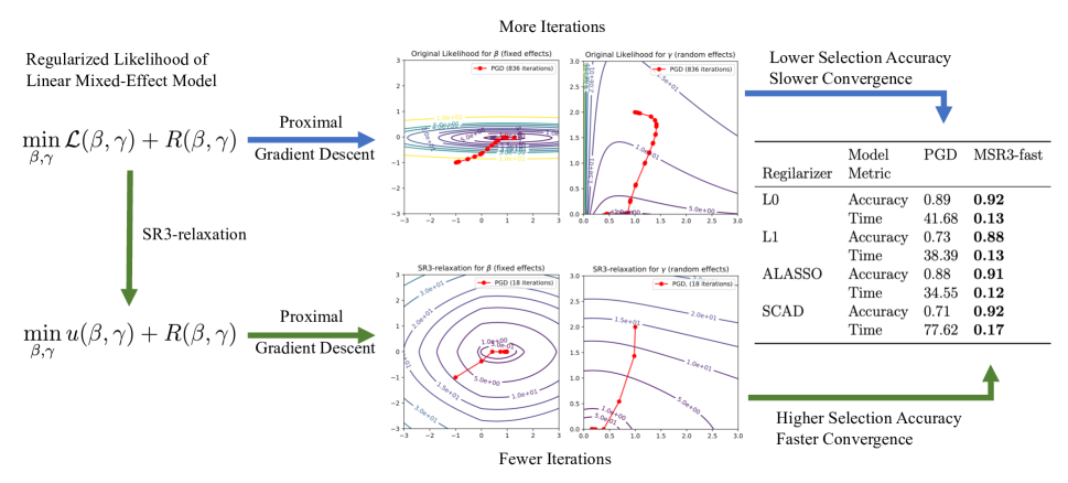
Figure 1: Selection of fixed and random effects for LME likelihoods $\mathcal{L}$ using ‘regularization-agnostic’ framework and its SR3 extension using four regularizers. SR3 relaxation accelerates algorithmic converge (middle panel), and gives better robustness and improved performance on synthetic problems across regularizers (right panel)

.

In this work we develop a regularization-agnostic covariate selection strategy that (1) is fast and simple to implement, (2) provides robust models, and (3) is flexible enough to support most regularizers currently used in variable selection across different domains. The baseline approach uses the proximal gradient descent (PGD) method, which has been studied by the optimization community for over 40 years, but has not been widely used in LME covariate selection. We provide proximal operators for commonly used regularizers and show how to apply the PGD method to the nonconvex LME setting. In particular we apply the PGD method to four regularizers, including the $\ell_{0}$ regularizer, which does not admit local quadratic approximations and has not been used before for LME variable selection strategies.

We also develop a new meta-approach that can improve the performance of LME selection methods for any regularizer. Specifically, we extend sparse relaxed regularized regression (SR3) framework (Zheng et al. (2019)) to the LME setting. In linear regression, SR3 accelerates and improves the performance of regularization strategies by introducing auxiliary variables that decouple the accuracy and sparsity requirements for the model coefficients. We develop a conceptual and algorithmic approach necessary to extend the SR3 concept to LME. This development is necessary because the LME problem is nonlinear, nonconvex, and includes constraints on variance parameters. We show that the new approach yields superior results in terms of specificity and sensitivity of feature selection, and is also computationally efficient.

All new methods are implemented in an open-source library called pysr3, which fills a gap for python mixed-models selection tools in Python (Buscemi and Plaia (2019), Table 3). Our algorithms are 1-2 orders of magnitude faster than available LASSO-based libraries for mixed effects selection in R, see Table 3. pysr3 enables a standardized comparison of different methods in the LME setting, and makes both the PGD framework and its SR3 extension available to practitioners working with LME models.

2 Linear Mixed-Effects Models: Notation and Fundamentals

Mixed-effect models describe the relationship between an outcome variable and its predictors when the observations are grouped, for example in studies or clusters. To set the notation, consider $m$ groups of observations indexed by $i$, with sizes $n_{i}$, and the total number of observations equal to $n=n_{1}+n_{2}+\dots+n_{m}$. For each group, we have design matrices for fixed features $X_{i}\in\operatorname{\mathbb{R}}^{n_{i}\times p}$, and matrices of random features $Z_{i}\in\operatorname{\mathbb{R}}^{n_{i}\times q}$, along with vectors of outcomes $Y_{i}\in\operatorname{\mathbb{R}}^{n_{i}}$. Let $X=[X_{1}^{T},X_{2}^{T},\dots,X_{m}^{T}]^{T}$ and $Z=[Z_{1}^{T},Z_{2}^{T},\dots,Z_{m}^{T}]^{T}$. Following Patterson and Thompson (1971); Pinheiro and Bates (2000), we define a Linear Mixed-Effects (LME) model as

$$\begin{split}Y_{i}&=X_{i}\beta+Z_{i}u_{i}+\varepsilon_{i},\quad i=1\dots m\\ u_{i}&\sim\operatorname{\mathcal{N}}(0,\Gamma),\quad\Gamma\in\operatorname{\mathbb{S}}_{+}^{q}\\ \varepsilon_{i}&\sim\operatorname{\mathcal{N}}(0,\Lambda_{i}),\quad\Lambda_{i}\in\operatorname{\mathbb{S}}_{++}^{n_{i}}\end{split}$$ (1)

where $\beta\in\operatorname{\mathbb{R}}^{p}$ is a vector of fixed (mean) covariates, $u_{i}\in\operatorname{\mathbb{R}}^{q}$ are unobservable random effects assumed to be distributed normally with zero mean and the unknown covariance matrix $\Gamma$, and $\operatorname{\mathbb{S}}_{+}^{\nu}$ and $\operatorname{\mathbb{S}}_{++}^{\nu}$ are the sets of real symmetric $\nu\times\nu$ positive semi-definite and positive definite matrices, respectively. Matrices $Z_{i}$ encode a wide variety of models, including random intercepts ($Z_{i}$ are columns of 1’s that add $u_{i}$ to all datapoints from the $i$th study) and random slopes ($Z_{i}$ also scale $u_{i}$ according to the magnitude of a covarite), see e.g. Pinheiro and Bates (2006). In our study, we assume that the observation error covariance matrices $\Lambda_{i}$ are given and that the random effects covariance matrix is an unknown diagonal matrix, i.e., $\Gamma=\mathrm{Diag}\left(\gamma\right),\ \gamma\in\operatorname{\mathbb{R}}^{s}_{+}$.

Defining group-specific error terms $\omega_{i}=Z_{i}u_{i}+\varepsilon_{i}$, we get a compact formulation that recasts (1) as a correlated noise model:

$$\begin{split}Y_{i}=X_{i}\beta+\omega_{i},\quad\omega_{i}\sim\operatorname{\mathcal{N}}(0,\Omega_{i}(\Gamma)),\quad\Omega_{i}(\Gamma)=Z_{i}\Gamma Z_{i}^{T}+\Lambda_{i}.\end{split}$$ (2)

For brevity, we refer to $\Omega_{i}(\Gamma)$ as just $\Omega_{i}$. The reformulation (2) yields the following marginalized negative log-likelihood function of a linear mixed-effects model (Patterson and Thompson, 1971):

$$\begin{split}\operatorname{\mathcal{L}}_{ML}(\beta,\Gamma):=\sum_{i=1}^{m}\frac{1}{2}(y_{i}-X_{i}\beta)^{T}\Omega_{i}^{-1}(y_{i}-X_{i}\beta)+\frac{1}{2}\ln{\det{\Omega_{i}}}.\end{split}$$ (3)

Maximum likelihood estimates for $\beta$ and $\Gamma$ are obtained by solving the optimization problem

$$\begin{split}\min_{\beta,\Gamma}&\ \operatorname{\mathcal{L}}_{ML}(\beta,\Gamma)\quad\mbox{s.t.}\quad\ \Gamma\in\operatorname{\mathbb{S}}_{+}^{q}.\end{split}$$ (4)

At this point, we bring in three basic definitions from variational analysis Rockafellar and Wets (2009).

Definition 1 (Epigraph and level sets).

The epigraph of a function $f:\mathbb{R}^{n}\rightarrow\mathbb{R}\cup\{\infty\}$ is defined as

$$\operatorname{epi}f=\{(x,\alpha):f(x)\leq\alpha\}.$$

For a given $\alpha$, the $\alpha$-level set of $f$ is defined as

$$\text{lev}_{\alpha}f=\{x:f(x)\leq\alpha\}.$$

Definition 2 (Lower semicontinuity and level-boundedness).

A function $f:\mathbb{R}^{n}\rightarrow\mathbb{R}\cup\{\infty\}$ is lower semicontinous (lsc) when $\operatorname{epi}f$ is closed, and level-bounded when all level sets $\text{lev}_{\alpha}f$ are bounded.

Definition 3 (Convexity).

A function $f:\mathbb{R}^{n}\rightarrow\mathbb{R}\cup\{\infty\}$ is convex when $\operatorname{epi}f$ is a convex set. Equivalently,

$$f(\lambda x+(1-\lambda)y)\leq\lambda f(x)+(1-\lambda)f(y)\quad\forall x,y,\lambda\in(0,1).$$

Definition 4 (Weak convexity).

A function $f:\mathbb{R}^{n}\rightarrow\mathbb{R}\cup\{\infty\}$ is $\lambda$-weakly convex $f(\cdot)+\frac{\lambda}{2}\|\cdot\|^{2}$ is convex.

The negative log likelihood (4) is nonlinear and nonconvex, and requires an iterative numerical solver. However, it is convex with respect to $\beta$, and weakly convex with respect to $\gamma$, with a weak convexity constant $\overline{\lambda}$ computed in (Sholokhov, 2022, Section 5.1) . The expected value of the posterior mode $\beta$ given $\Gamma$ has a closed form representation of the form

$$\beta(\Gamma)=\operatorname*{\mathrm{argmin}}_{\beta}\operatorname{\mathcal{L}}(\beta,\Gamma)=\left(\sum_{i=1}^{m}X_{i}^{T}\Omega_{i}^{-1}X_{i}\right)^{-1}\sum_{i=1}^{m}X_{i}^{T}\Omega_{i}^{-1}y_{i}.$$

By using the simplification $\Gamma=\mathrm{Diag}\left(\gamma\right)$, we obtain the problem

$$\begin{split}\min_{\beta\in\operatorname{\mathbb{R}}^{p},\gamma\in\operatorname{\mathbb{R}}^{q}_{+}}&\ \operatorname{\mathcal{L}}(\beta,\gamma):=\operatorname{\mathcal{L}}_{ML}(\beta,\mathrm{Diag}\left(\gamma\right))\end{split}$$ (5)

In this setting, when an entry $\gamma_{j}$ takes the value $0$ the corresponding coordinates of all random effects $u_{ij}$ are identically $0$ for all $i$.

Verification of the existence to solutions to (5) and, more generally, (4) follows from the work of Zheng et al. (2021). Standalone proofs for the existence of minimizers are developed in (Sholokhov, 2022, Theorem 1), and extended to the presence of regularizers in (Sholokhov, 2022, Theorem 2).

In this paper we focus the case where $\Gamma$ is diagonal, and all $\Lambda_{i}$ are known (see (5)), following the meta-analysis use-case (Zheng et al., 2021). Our numerical experiments show that we get better selection methods by trading complexity of the problem (4) for for the simplicity and robustness of the problem (5).

2.1 Prior Work on Feature Selection for Mixed-Effects Models

Variable (feature) selection seeks to select or rank the most important predictors in a dataset in order to get a parsimonious model at a minimal cost to prediction quality. If the desired number of coefficients $k$ is given, then the feature selection problem can be formulated as the minimization of a loss function $f(\theta)$ (e.g. the negative log-likelihood) subject to a zero-norm constraint:

$$\begin{split}&\min_{\theta}f(\theta)\quad\mbox{ s.t. }\quad\|\theta\|_{0}\leq k\end{split}$$ (6)

where $\|\theta\|_{0}$ denotes the number of nonzero entries in $\theta$, see panel (c) of Figure 2.

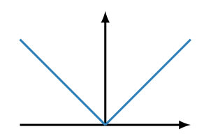
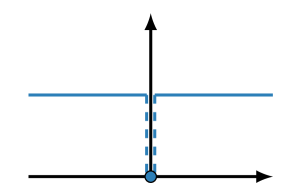
(a) $\ell_{1}$	(b) $\ell_{1/2}$	(c) $\ell_{0}$

Figure 2: Common convex and non-convex regularizers used for feature selection.

The constraint in (LABEL:eq:general_feature_selection_zero_norm) is combinatorial, and a common workaround is to relax it to a one-norm constraint, with $\|\theta\|_{1}$ equal to the sum of absolute values of the entries of $\theta$. The best-known example of this approach is the least absolute square shrinkage operator (LASSO) studied by Tibshirani (1996b) for linear regression, see panel (a) of Figure 2.

Feature selection for LMEs is more difficult than for linear regression models. In linear regression the observations are independent, whereas in mixed-effects setup they are generally correlated. In addition, LMEs have both mean effect variables $\beta$ as well as random variance variables $\Gamma$. The shrinkage operator approach for linear regression (Tibshirani, 1996b) was first adapted to the problem of feature selection for the fixed effects in mixed-effect models by Lan (2006). The removal of a random effect from the model requires the elimination of an entire row and column from $\Gamma$. To make the problem more tractable, Chen and Dunson (2003) reparamtrized $\Gamma$ through a modified Cholesky decomposition $\Gamma(D,L):=DLL^{T}D$, where $D$ is a diagonal matrix and $L$ is a lower-triangular matrix with ones on the main diagonal, and focused on selecting elements of $D$. Based on this idea, Bondell et al. (2010) extended the Adaptive LASSO regularizer (Lan (2006); Xu et al. (2015)) to mixed-effects setting using the objective

$$\operatorname{\mathcal{L}}(\beta,\Gamma(D,L))+\lambda\left(\sum_{i=1}^{p}\left|\frac{\beta_{i}}{\hat{\beta}_{i}}\right|+\sum_{j=1}^{q}\frac{D_{ii}}{\hat{D_{ii}}}\right),$$

where $\hat{\beta}$ and $\hat{D}$ are the solution of a non-penalized maximum likelihood problem. Ibrahim et al. (2011b) use a similar approach, penalizing non-zero elements $\Gamma_{ij}$ directly. Other methods that use Adaptive LASSO for simultaneous selection of fixed and random effects are Lin et al. (2013a); Fan et al. (2014); Pan and Shang (2018). Adaptive LASSO is available to practitioners via R packages glmmLasso (Groll and Tutz (2014)) and lmmLasso(Schelldorfer et al. (2011)).

A popular nonconvex regularizer used for feature selection is smoothed clipped absolute deviation (SCAD) Fan and Li (2001). The adaptation of the SCAD penalty to select both fixed and random features in linear mixed models was developed by Fan and Li (2012). SCAD was also used by Chen et al. (2015) for selecting fixed effects and establishing the existence of random effects in ANOVA-type models. Finally, Ghosh and Thoresen (2018) studied SCAD regularization for selecting mean effects in high-dimensional genomics problems.

To better compare methods, we need to consider the regularization parameter and how it is tuned. The output of a shrinkage model depends on this tuning parameter, typically called $\lambda$. The entire range of possible $\lambda$ values is captured by the notion of a “$\lambda$-path in the model space”, with the best parameter and the final model chosen using information criteria. According to Müller et al. (2013), the most widely used information criterion is the marginal AIC criterion (Vaida and Blanchard (2005)):

$$\begin{split}AIC=2\operatorname{\mathcal{L}}(\hat{\theta})+2\alpha_{n}(p+q)\end{split}$$ (7)

where $\hat{\theta}$ includes all the estimated parameters $(\beta,\Gamma)$, and $\alpha_{n}=n(n-p-q-1)$ for a finite sample case (Sugiura (1978)). Alternatively, LASSO-type methods (Bondell et al. (2010); Ibrahim et al. (2011b)) use a BIC-type information criterion:

$$\begin{split}BIC=2\operatorname{\mathcal{L}}(\hat{\theta})+\log(n)(p+q).\end{split}$$ (8)

BIC performs well in practice, but does not have theoretical guarantees (Schelldorfer et al. (2011)).

3 Algorithms for Feature Selection

To develop our feature selection approach, we add a regularizer to model (5):

$$\begin{split}\min_{x}&\operatorname{\mathcal{L}}(x)+R(x)+\delta_{\mathcal{C}}(x),\end{split}$$ (9)

where $x=(\beta,\gamma)$, $\mathcal{C}:=\operatorname{\mathbb{R}}^{p}\times\operatorname{\mathbb{R}}^{q}_{+}$, $R:\operatorname{\mathbb{R}}^{P}\times\operatorname{\mathbb{R}}^{q}_{+}\rightarrow{\overline{\operatorname{\mathbb{R}}}}_{+}:=\operatorname{\mathbb{R}}_{+}\cup\{+\infty\}$ is a lower semi-continuous (lsc) regularization term, and $\delta_{\mathcal{C}}$ is the convex indicator function

$$\delta_{\mathcal{C}}(x):=\begin{cases}0,&x\in\mathcal{C}\\ +\infty,&x\not\in\mathcal{C}.\end{cases}$$

By Theorem LABEL:thm:basic_existence2, solutions to (9) always exist. The most common regularizers are separable:

$$R(x)=\sum_{i=1}^{p}r_{i}(x_{i}).$$ (10)

Typical choices for the component functions $r_{i}$ are given in Table 1.

3.1 Variable Selection via Proximal Gradient Descent

Since $\operatorname{\mathcal{L}}$ is differentiable on its domain, the Proximal Gradient Descent (PGD) Algorithm offers a simple numerical strategy for estimating first-order stationary points for (9) when the application of the proximal operator to $\alpha R+\delta_{\mathcal{C}}$ is computationally tractable. The proximal operator for $\alpha R+\delta_{\mathcal{C}}$ is defined as the mapping

$${\mathrm{prox}}_{\alpha R+\delta_{\mathcal{C}}}(z):=\operatorname*{\mathrm{argmin}}_{y\in\mathcal{C}}\ R(y)+\frac{1}{2\alpha}\|y-z\|_{2}^{2},$$

and the PGD iteration is given by

$$x^{+}={\mathrm{prox}}_{\alpha R+\delta_{\mathcal{C}}}(x-\alpha\nabla\operatorname{\mathcal{L}}(x)),$$

where $\alpha$ is a stepsize. When $R(x)$ has the form given in (10), we have

$${\mathrm{prox}}_{R}(z)=({\mathrm{prox}}_{r}(z_{1}),\dots,{\mathrm{prox}}_{r}(z_{q})).$$

​​Regularizer	$r(x)$, $x\in\operatorname{\mathbb{R}}$	${\mathrm{prox}}_{\alpha r}(z)$
LASSO ($\ell_{1}$) (Tibshirani (1996a))	$|x|$	$\operatorname*{\mathrm{sign}}(z)(|z|-\alpha)_{+}$
A-LASSO (Fan and Li (2001))	$\bar{w}|x|$, $\bar{w}\geq 0$	$\operatorname*{\mathrm{sign}}(z)(|z|-\alpha\bar{w})_{+}$
SCAD (Fan (1997))	$\begin{cases}\sigma|x|,&|x|\leq\sigma\\ \frac{-x^{2}+2\rho\sigma x-\sigma^{2}}{2(\rho-1)},&\sigma<|x|<\rho\sigma\\ \frac{\sigma^{2}(\rho+1)}{2},&|x|>\rho\sigma\end{cases}$	$\begin{cases}\operatorname*{\mathrm{sign}}(z)(|z|-\sigma\alpha)_{+},&|z|\leq\sigma(1+\alpha)\\ \frac{(\rho-1)z-\operatorname*{\mathrm{sign}}(z)\rho\sigma\alpha}{\rho-1-\alpha},&\sigma(1+\alpha)<|z|\\ &\quad\leq\max(\rho,1+\alpha)\sigma\\ z,&|z|>\max(\rho,1+\alpha)\sigma\end{cases}$
$\delta_{\|x\|_{0}\leq k}$ ($\ell_{0}$ ball)	$\begin{cases}0,&\#\{|x_{i}|\neq 0\}\leq k\\ \infty,&\text{ otherwise}\end{cases}$	keep $k$ largest $|x_{i}|$, set the rest to 0

Table 1: Proximal operators for commonly used sparsity-promoting regularizers.

Table 1 provides closed form expressions for the proximal operators of commonly used regularizers. For all of these cases, the following theorem gives closed form expressions for ${\mathrm{prox}}_{\alpha R+\delta_{\mathcal{C}}}(z)$.

Theorem 1 (${\mathrm{prox}}$ for bounded $\gamma$).

Consider the regularizers from the Table 1. Add a constraint on $\gamma$ of the form

$$0\leq\gamma\leq\bar{\gamma},$$

which has the positive orthant as a special case (i.e. $\bar{\gamma}=\infty$). We have the following results.

1. For CAD, SCAD, we have for all $i$ that

   $${\mathrm{prox}}_{(\alpha r+\delta_{[0,{\bar{\gamma}}]})}(\gamma_{i})=\begin{cases}{\mathrm{prox}}_{\alpha r}(\gamma_{i}),&0\leq\gamma_{i}<\bar{\gamma}\\ \bar{\gamma},&\gamma_{i}\geq\bar{\gamma}\\ 0,&\text{ otherwise}\end{cases}$$

2. For LASSO, A-LASSO we have for all $i$ that

   $${\mathrm{prox}}_{(\alpha r+\delta_{[0,{\bar{\gamma}}]})}(\gamma_{i})=\begin{cases}{\mathrm{prox}}_{\alpha r}(\gamma_{i}),&0\leq\gamma_{i}<\bar{\gamma}+\alpha\\ \bar{\gamma},&\gamma_{i}\geq\bar{\gamma}+\alpha\\ 0,&\text{ otherwise}\end{cases}$$

3. For $R(\cdot)=\delta_{{\mathrm{lev}_{\left\|\cdot\right\|_{0}}(k)}}$ the ${\mathrm{prox}}_{\alpha R+\delta_{\mathcal{C}}}(\gamma)$ can be evaluated by taking $k$ largest coordinates of $\gamma$ such that $0\leq\gamma_{i}\leq\bar{\gamma}$, and setting the remainder to $0$.

The proof of the Theorem 1 is provided in Appendix A.2. The PGD algorithm is detailed in Algorithm 1. The algorithm’s step-size $\alpha$ depends on the Lipschitz constant; an upper-bound has been estimated as in Appendix A.3. In practice, $\alpha$ is computed using a line-search, since the available estimate of $L$ is very conservative.

1 $x=x_{0}$, $\alpha<\frac{1}{L}$, where $\operatorname{\mathcal{L}}$ is $L$-Lipschitz

2 while not converged do

3       $x^{+}={\mathrm{prox}}_{\alpha R+\delta_{\mathcal{C}}}(x-\alpha\nabla\operatorname{\mathcal{L}}(x))$;

4      

5 end while

Algorithm 1 Proximal Gradient Descent for Linear Mixed-Effect Models

The main advantages of Algorithm 1 are its simplicity and flexibility. The main loop needs only the gradient and prox operator, and the structure of the algorithm is independent of the choice of regularizer $R$. Algorithm 1 converges under weak assumptions, in particular neither the objective nor the regularizer need to be convex (Beck, 2017; Attouch et al., 2013).

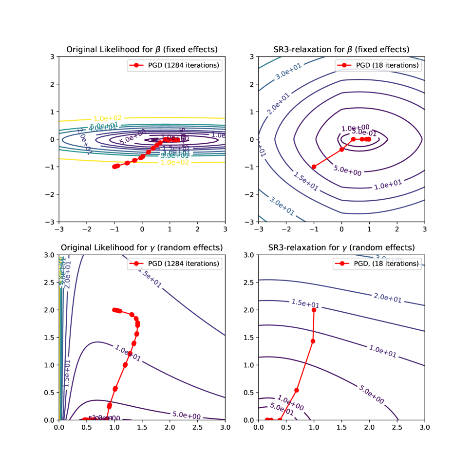
Figure 3: Proximal Gradient Descent (PGD) for (14) converges far faster than for (9), because the SR3-value function $u_{\eta}$ yields more spherical level-sets than original likelihood for both convex components $\beta$ (first row) and non-convex components $\gamma$ (second row).

3.2 Variable Selection via MSR3

To develop an approach that is both more efficient and accurate, we extend the SR3 regularization of Zheng et al. (2019) to LMEs. We call the extension MSR3, since we are focusing on mixed effects models. Starting with the regularized likelihood (9) we introduce auxiliary parameters designed to discover the fixed and random features:

$$\begin{split}\min_{x,w}&\operatorname{\mathcal{L}}(x)+R(w)+\delta_{\mathcal{C}}(x)+\kappa_{\eta}(x-w),\end{split}$$ (11)

where $\kappa_{\eta}$ penalizes deviations between $x$ and $w$, and also guarantees that the objective is convex with respect to the $\gamma$ components of $x$:

$$\kappa_{\eta}(\beta,\gamma)=\frac{\eta}{2}\|\beta\|^{2}+\frac{\overline{\lambda}+\eta}{2}\|\gamma\|^{2}.$$ (12)

Here, $\overline{\lambda}$ is the weak convexity constant for the objective (11) with respect to $\gamma$. As $\eta\uparrow\infty$, the extended objective (11) converges in an epigraphical sense to the original objective (9). However, feature selection accuracy does not require this continuation, and a fixed value, e.g. $\eta=1$, can be used (Zheng et al., 2019).

To understand the algorithm and logic behind the objective (11), we define a value function $u_{\eta}(w)$ and the solution set $S_{\eta}(w)$:

$$\begin{split}u_{\eta}(w)&=\min_{x}\ \operatorname{\mathcal{L}}(x)+\delta_{\mathcal{C}}(x)+\kappa_{\eta}(x-w)\\ S_{\eta}(w)&=\operatorname*{\mathrm{argmin}}_{x}\operatorname{\mathcal{L}}(x)+\delta_{\mathcal{C}}(x)+\kappa_{\eta}(x-w)\end{split}$$ (13)

Substituting (13) into (11) the problem transforms into the problem of optimizing a regularized value function:

$$\begin{split}\min_{w}u_{\eta}(w)+R(w)\end{split}$$ (14)

Thus at a conceptual level, the original regularized likelihood (9) has been transformed through relaxation and partial minimization to a mirrored problem (14) with the same regularizer. Problem (14) attempts to find sparse $w$ that are small with respect to $u_{\eta}$.

The function $u_{\eta}$ has a closed form solution for linear regression Zheng et al. (2019). However, in both the linear regression context of Zheng et al. (2019) and in the LME context studied here, we need only compute $S_{\eta}(w)$ in order to optimize (14). The function $u_{\gamma}$ is well-defined (Sholokhov, 2022, Theorem 9), differentiable (Sholokhov, 2022, Theorem 11), and Lipschitz continuous (Sholokhov, 2022, Corollary 15), and we have a closed form solution for the derivative:

$$\nabla u_{\eta}(w)=\nabla_{w}k_{\eta}(x-w)|_{x=S_{\eta}(w)},$$

where $\nabla_{w}k_{\eta}(x-w)$ is computed directly from (12).

The advantages of solving (14) over (9) come from $u_{\eta}(w)$ having nearly spherical level-sets while keeping the position of minima close to those of $\operatorname{\mathcal{L}}(x)$. While this effect was extensively studied for a quadratic loss function in the original work (Zheng et al. (2019)), we provide empirical evidence that suggests that it also extends to more general non-linear functions, specifically to the marginal likelihood. In Figure 3, we plot the level-sets of $\operatorname{\mathcal{L}}(x)+\|x\|_{1}$ (left column) and $u(w)+\|w\|_{1}$ (right column) for the same mixed-effect problem. The more spherical geometry of the latter allows the Algorithm 3 to converge in 21 iterations, whereas Algorithm 1 takes 1284 iterations. The difference is most pronounced when the minimum sits on the boundary of the feasible set, which is always the case for the variable selection problems with true sparse support.

We apply PGD to optimize the value function $u_{\eta}(w)$ which yields the iteration of the form

$$\begin{split}w^{+}={\mathrm{prox}}_{\alpha^{-1}R}(w-\alpha\nabla u_{\eta}(w))\end{split}$$ (15)

Because of the results stated above, all components of the iteration (15) are well-defined. To get a deeper intuition for Algorithm 2 we make the following remark.

Remark 1 (Equivalence of Algorithms).

Algorithm 2 is equivalent to (15).

Proof.

We extend the relationship studied by Zheng et al. (2019) to the case of $x=(\beta,\gamma)$. Specifically, we define $\alpha$ to be block-specific:

$$\alpha=[\underbrace{\eta^{-1},\dots,\eta^{-1}}_{p},\underbrace{(\eta+\overline{\lambda})^{-1},\dots(\eta+\overline{\lambda})^{-1}}_{q}]$$

so that we have

$$\begin{split}\nabla u_{\eta}(w)=\alpha\odot(\overline{x}-w)|_{\overline{x}=S_{\eta}(w)}\end{split}$$ (16)

where “$\odot$” denotes the Hadamard or element-wise product. Substituting (16) into (15), we see that the iteration (15) is equivalent to the alternating minimization scheme outlined in the Algorithm 2. ∎

1 $w=w_{0}$

2 while not converged do

3       $x^{+}=\arg\min_{x}\operatorname{\mathcal{L}}(x)+\delta_{\mathcal{C}}(x)+\kappa_{\eta}(x-w)$

4       $w^{+}={\mathrm{prox}}_{\alpha\odot R}(x^{+})$

5 end while

Algorithm 2 Proximal Gradient Descent for Value Function

The alternating strategy is best suited for the simpler context of Zheng et al. (2019), where the $x^{+}$ update has a closed form solution. In the case of (11), the regularized loss is convex in $x$ because of the structure of $\kappa$, but is still nonlinear, and requires an iterative algorithm.

3.3 Interior Point Method for Inequality Constraints

In order to solve for the $x^{+}$ update in line 2 of Algorithm 2, we must optimize a convex loss with linear inequality constraints. For a fixed $w=(\hat{\beta},\hat{\gamma})$, we solve

$$\min_{\beta,\gamma}\mathcal{L}(\beta,\gamma)+\kappa_{\eta}(\beta-\hat{\beta},\gamma-\hat{\gamma})\quad\mbox{s.t.}\quad 0\leq\gamma.$$ (17)

This problem is well suited for an interior point method (Kojima et al., 1991; Nesterov and Nemirovskii, 1994; Wright, 1997). First, we relax the inequality constraint $0\leq\gamma$ via a log-barrier penalty, obtaining a minimization problem for a new objective $\mathcal{L}_{\mu,\eta}$:

$$\begin{split}\min_{\beta,\gamma}&\left\{\mathcal{L}_{\mu,\eta}(\beta,\gamma):=\mathcal{L}(\beta,\gamma)+\kappa_{\eta}(\beta-\hat{\beta},\gamma-\hat{\gamma})-\mu\sum_{i=1}^{q}\ln(\gamma_{i})\right\}.\end{split}$$ (18)

The log-barrier penalty approximates the indicator function to the positive orthant as $\mu$ decreases:

$$\lim_{\mu\downarrow 0}-\mu\ln(\gamma)=\delta_{\mathbb{R}^{n}_{+}}(\gamma).$$

The penalty (homotopy) parameter $\mu$ is progressively decreased to $0$ as the algorithm proceeds as described below. in the limit minimizing $\mathcal{L}_{\eta,\mu}$ gives the right $x^{+}$ update in Algorithm 2. The existence of solutions for the problem (18) for any positive $\mu$ is shown in (Sholokhov, 2022, Theorem 5), and the convergence of solutions to the MSR3 solution as $\mu\downarrow 0$ is shown in (Sholokhov, 2022, Theorem 7). Finally, (Sholokhov, 2022, Theorem 6) shows that the MSR3 relaxation is consistent with respect to the barrier, so that as the MSR3 parameter $\eta\uparrow\infty$, limit points of global solutions to the former are global solutions to the latter. However, we do not use $\eta$-continuation in the applications considered here.

For $\gamma>0$, the necessary optimality conditions for $\mathcal{L}_{\mu,\eta}$ in $\gamma$ give us the relation

$$\begin{split}\nabla_{\gamma}\mathcal{L}_{\mu,\eta}(\beta,\gamma)=\nabla_{\gamma}\operatorname{\mathcal{L}}(\beta,\gamma)+(\overline{\lambda}+\eta)(\gamma-\hat{\gamma})-\mu\mathrm{Diag}\left(\gamma\right)^{-1}\mathbf{1}=0,\end{split}$$ (19)

where $\mathbf{1}$ is the vector of all ones of the appropriate dimension. By setting

$$v=\nabla_{\gamma}\mathcal{L}_{\mu,\eta}(\beta,\gamma)+(\overline{\lambda}+\eta)(\gamma-\hat{\gamma}),$$

we can rewrite this equation as

$$\begin{split}v\odot\gamma-\mu\mathbf{1}=0,\end{split}$$ (20)

where $\mathbf{1}$ is the vector of all ones of the appropriate dimension. The complete set of optimality conditions for (18) can now be written as

$$\begin{split}G_{\mu,\eta}(v,\beta,\gamma)&:=\begin{bmatrix}v\odot\gamma-\mu\mathbf{1}\\ \nabla_{\beta}\operatorname{\mathcal{L}}(\beta,\gamma)+\eta(\beta-\hat{\beta})\\ \nabla_{\gamma}\operatorname{\mathcal{L}}(\beta,\gamma)+(\overline{\lambda}+\eta)(\gamma-\hat{\gamma})-v\end{bmatrix}=0.\end{split}$$ (21)

We then apply Newton’s method to (21), so in each iteration the search direction $[\Delta v,\Delta\beta,\Delta\gamma]$ solves the linear system

$$\begin{split}\nabla G_{\mu,\eta}(v,\beta,\gamma)\begin{bmatrix}\Delta v\\ \Delta\beta\\ \Delta\gamma\end{bmatrix}=-G_{\mu,\eta}(v,\beta,\gamma).\end{split}$$ (22)

where

$$\begin{split}\nabla G_{\mu,\eta}(v,\beta,\gamma)=\begin{bmatrix}\mathrm{Diag}\left(\gamma\right)&0&\mathrm{Diag}\left(v\right)\\ 0&\nabla^{2}_{\beta\beta}\operatorname{\mathcal{L}}+\eta I&\nabla^{2}_{\beta\gamma}\operatorname{\mathcal{L}}\\ -I&\nabla^{2}_{\gamma\beta}\operatorname{\mathcal{L}}&\nabla^{2}_{\gamma\gamma}\operatorname{\mathcal{L}}+(\eta+\overline{\lambda})I\end{bmatrix}\end{split}$$ (23)

and we have used the fact that $v\odot\gamma=\mathrm{Diag}\left(v\right)\gamma=\mathrm{Diag}\left(\gamma\right)v$. The exact formulae for the derivatives of $\operatorname{\mathcal{L}}$ are provided in the Appendix A.1.

The general structure of the algorithm is as follows. Given a search direction $[\Delta v^{(k)},\Delta\beta^{(k)},\Delta\gamma^{(k)}]$, choose a step of size $\alpha_{k}>0$ so that the update

$$\begin{pmatrix}v^{(k+1)}\\ \beta^{(k+1)}\\ \gamma^{(k+1)}\end{pmatrix}=\begin{pmatrix}v^{(k)}\\ \beta^{(k)}\\ \gamma^{(k)}\end{pmatrix}+\alpha_{k}\begin{pmatrix}\Delta v^{(k)}\\ \Delta\beta^{(k)}\\ \Delta\gamma^{(k)}\end{pmatrix}$$

satisfies the conditions

$$\begin{split}\text{{Positivity:}}\qquad&\gamma^{(k+1)}>0,\ v^{(k+1)}>0\\ \text{{Sufficient Descent:}}\qquad&\|G_{\mu}(v^{(k+1)},\beta^{(k+1)},\gamma^{(k+1)})\|\leq 0.99\|G_{\mu}(v^{(k)},\beta^{(k)},\gamma^{(k)})\|.\end{split}$$ (24)

At each iteration the relaxation parameter $\mu$ is updated by the formula

$$\begin{split}\mu^{(k+1)}={v^{(k)}}^{T}\gamma^{(k)}/q,\end{split}$$ (25)

where ${v^{(k)}}^{T}\gamma^{(k)}$ is the duality gap at iteration $k$. The algorithm terminates when the criteria

$$\begin{split}\begin{aligned} \|G_{\mu,\eta}(v^{(k+1)},\beta^{(k+1)},\gamma^{(k+1)})\|&\leq\text{{tol}}\\ \mu&\leq\text{{tol}}\end{aligned}\end{split}$$ (26)

are both satisfied, so the interior point problem is nearly stationary, and closely approximates the original problem (17).

Positive Approximation of the Hessian

For many datasets the weak convexity constant $\overline{\lambda}$ for $\gamma$ can be extremely large or even uncomputable. In this case, setting a smaller value $\overline{\lambda}$ is likely to force $\nabla^{2}_{\gamma\gamma}\operatorname{\mathcal{L}}(\beta,\gamma)$ to be negative-definite. Negative definite Hessians may hamper the convergence of second-order methods (Nocedal and Wright (2006)). We prevent this effect by using the Fisher information matrix regarding to $\gamma$ as the positive definite approximation of the Hessian. Here, we provide the derivation of the Fisher information matrix formula.From the fact that,

$$\mathbb{E}\left[(X_{i}\beta-Y_{i})(X_{i}\beta-Y_{i})^{T}\right]=\mathbb{E}\left[(Z_{i}u_{i}+\epsilon_{i})(Z_{i}u_{i}+\epsilon_{i})^{T}\right]=\Omega_{i}$$

we know,

$$\mathbb{E}\left[\nabla^{2}_{\gamma\gamma}\operatorname{\mathcal{L}}(\beta,\gamma)\right] =\mathbb{E}\left[\sum_{i=1}^{m}\left(Z_{i}^{T}\Omega_{i}^{-1}(X_{i}\beta-Y_{i})(X_{i}\beta-Y_{i})^{T}\Omega_{i}^{-1}Z_{i}\right)\circ(Z_{i}^{T}\Omega_{i}^{-1}Z_{i})-\frac{1}{2}(Z_{i}^{T}\Omega_{i}^{-1}Z_{i})^{\circ 2}\right]$$

$$=\sum_{i=1}^{m}\left(Z_{i}^{T}\Omega_{i}^{-1}\mathbb{E}\left[(X_{i}\beta-Y_{i})(X_{i}\beta-Y_{i})^{T}\right]\Omega_{i}^{-1}Z_{i}\right)\circ(Z_{i}^{T}\Omega_{i}^{-1}Z_{i})-\frac{1}{2}(Z_{i}^{T}\Omega_{i}^{-1}Z_{i})^{\circ 2}$$

$$=\sum_{i=1}^{m}\left(Z_{i}^{T}\Omega_{i}^{-1}Z_{i}\right)\circ(Z_{i}^{T}\Omega_{i}^{-1}Z_{i})-\frac{1}{2}(Z_{i}^{T}\Omega_{i}^{-1}Z_{i})^{\circ 2}=\frac{1}{2}\sum_{i=1}^{m}(Z_{i}^{T}\Omega_{i}^{-1}Z_{i})^{\circ 2}$$

And we use $\mathbb{E}\left[\nabla^{2}_{\gamma\gamma}\operatorname{\mathcal{L}}(\beta,\gamma)\right]$ as the positive definite approximation of $\nabla^{2}_{\gamma\gamma}\operatorname{\mathcal{L}}(\beta,\gamma)$.

3.4 Relaxation and Efficient Algorithms: MSR3 and MSR3-Fast

While algorithm (2) is modular, it requires solving a nonlinear optimization problem in $x=(\beta,\gamma)$ for each single update of $w=(\hat{\beta},\hat{\gamma})$. To make the implementation as efficient as possible, we designed a more balanced updating scheme, that alternates Newton iterations as described in the interior point algorithm with $w$ updates. We update $w$ whenever we are sufficiently close to the ‘central path’ in the interior point method, a condition that can be checked rigorously using optimality conditions.

1 $\alpha\leftarrow 1$, $\texttt{progress}\leftarrow\textbf{True}$

2 $\beta^{+},\tilde{\beta}^{+}\leftarrow\beta_{0}$;  $\gamma^{+},\tilde{\gamma}^{+}\leftarrow\gamma_{0}$;  $v^{+}\leftarrow 1\in\operatorname{\mathbb{R}}^{q}$;  $\mu\leftarrow\frac{{v^{+}}^{T}\gamma^{+}}{10q}$

3 while iter $<$ max_iter  and  $\|G_{\eta,\mu}(\beta^{+},\gamma^{+},v^{+})\|$ $>$ tol  and  progress

4 do

5       $\beta\leftarrow\beta^{+}$;  $\gamma\leftarrow\gamma^{+}$;  $\tilde{\beta}\leftarrow\tilde{\beta}^{+}$;  $\tilde{\gamma}\leftarrow\tilde{\gamma}^{+}$

6       $[dv,d\beta,d\gamma]\leftarrow\nabla G_{\eta,\mu}((\beta,\gamma,v),(\tilde{\beta},\tilde{\gamma}))^{-1}G_{\eta,\mu}((\beta,\gamma,v),(\tilde{\beta},\tilde{\gamma}))$ // Newton Iteration

7       $\alpha\leftarrow 0.99\times\min\left(1,-\frac{\gamma_{i}}{d\gamma_{i}},\forall i:\ d\gamma_{i}<0\right)$

8       $\beta^{+}\leftarrow\beta+\alpha d\beta$;  $\gamma^{+}=\gamma+\alpha d\gamma$;  $v^{+}\leftarrow v+\alpha dv$

9       if $\|\gamma^{+}\odot v^{+}-q^{-1}{\gamma^{+}}^{T}v^{+}\mathbf{1}\|>0.5q^{-1}{v^{+}}^{T}\gamma^{+}$ then

10             continue // Keep doing Newton iterations

11            

12       end if

13      else

14             $\tilde{\beta}^{+}={\mathrm{prox}}_{\alpha R}(\beta^{+})$;   $\tilde{\gamma}^{+}={\mathrm{prox}}_{\alpha R+\delta_{\operatorname{\mathbb{R}}_{+}}}(\gamma^{+})$;   $\mu=\frac{1}{10}\frac{{v^{+}}^{T}\gamma^{+}}{q}$ // Near central path

15       end if

16      progress = ($\|\beta^{+}-\beta\|\geq\text{tol}$ or $\|\gamma^{+}-\gamma\|\geq\text{tol}$ or $\|\tilde{\beta}^{+}-\tilde{\beta}\|\geq\text{tol}$ or $\|\tilde{\gamma}^{+}-\tilde{\gamma}\|\geq\text{tol}$)

17 end while

return $\tilde{\beta}$, $\tilde{\gamma}$

Algorithm 3 MSR3 (Proximal Gradient Descent for the Value function)

4 Verifications

4.1 MSR3 for Covariate Selection

	Model	PGD	MSR3	MSR3-fast
Regilarizer	Metric
L0	Accuracy	0.89	0.92	0.92
	Time	41.68	88.54	0.13
L1	Accuracy	0.73	0.88	0.88
	Time	38.39	9.13	0.13
ALASSO	Accuracy	0.88	0.92	0.91
	Time	34.55	65.19	0.12
SCAD	Accuracy	0.71	0.93	0.92
	Time	77.62	84.67	0.17

Table 2: Comparison of performance of algorithms measured as accuracy of selecting the correct covariates and run-time. The L0 strategy stands out over other standard regularizers. MSR3 improves performance significantly for all regularizers, while MSR3-fast improves convergence speed while preserving the accuracy of MSR3. More detailed results are in the Table 4 of Appendix B.1.

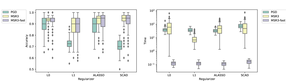
Figure 4: Feature selection accuracy and execution time in seconds for PGD and MSR3 with various regularizers. MSR3-Fast has the same accuracy as MSR3 and significantly decreases computation time.

In this section we show the performance of the ‘regularization-agnostic’ feature selection method, and also show that MSR3 improves performance across different regularization strategies. Specifically, we compare the feature selection accuracy and numerical efficiency of Algorithm 1 and 3 with LASSO, A-LASSO, CAD, SCAD, and L0.

Problem setup.

In this experiment we take the number of fixed effects $p$ and random effects $q$ to be $20$. We set $\beta=\gamma=[\frac{1}{2},\frac{2}{2},\frac{3}{2},\dots,\frac{10}{2},0,0,0,\dots,0]$, i.e. the first 10 covariates are increasingly important and the last 10 covariates are not. The data is generated as

$$y_{i} =X_{i}\beta+Z_{i}u_{i}+\varepsilon_{i},\quad\varepsilon_{i}\sim\operatorname{\mathcal{N}}(0,0.3^{2}I)$$

$$X_{i} \sim\operatorname{\mathcal{N}}(0,I)^{p},\quad Z_{i}=X_{i}$$

$$u_{i} \sim\operatorname{\mathcal{N}}(0,\mathrm{Diag}\left(\gamma\right))$$

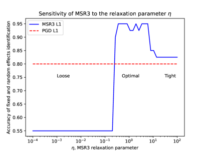
Figure 5: Dependence of model performance on the relaxation $\eta$ for a sample problem.

The data is generated for 9 groups, with the sizes of $[10,15,4,8,3,5,18,9,6]$ to capture a variety of group sizes. To estimate the uncertainty bounds, each experiment is repeated 100 times.

Parameter selection.

The regularization coefficient $\lambda$ and the relaxation coefficient $\eta$ were chosen to maximize a classic BIC criterion from Jones (2011). We used a golden bisection search to select between candidate $\lambda$ parameters and a grid search to select between $\eta$ candidate parameters.

Figure 5 shows the dependence of accuracy on the values of $\eta$ for the first problem from our test set. There are three distinct regions, corresponding to loose, optimal and tight levels of relaxations. When $\eta$ is small the relaxation term dominates, and the training does not progress far from the initial point (a fully dense vector 1 in this case). When the relaxation is tight, the level-sets of the problem converge to those of the original problem, and thus the minimizer. For the values in between, the relaxation significantly improves the model’s accuracy. These results are consistent with experiments in the sparse linear regression setting Zheng et al. (2019).

Results.

The results are presented in the Table 2. SR3 improves the selection accuracy of most regularization techniques from Table 1, showing a near-perfect performance, while converging two orders of magnitude faster in wall-clock time.

Comparison to other libraries

We compare performance of pysr3 to the performance R packages glmmLasso (Groll and Tutz (2014)) and lmmLasso(Schelldorfer et al. (2011)) – the functionally closest libraries available online. We evaluate their performance on the same set of problems and the parameters selection procedure as described above and compare it to SR3+LASSO. We tuned the hyperparameters of glmmLasso and lmmLasso by minimizing the BIC scores provided by the libraries. The results are presented in Table 3. Overall, SR3 executes, on average, 5 times faster in wall-clock time than glmmLasso and 60 times faster than lmmLasso and shows much higher accuracy of selecting correct fixed and random effects simultaneously. lmmLasso supports the diagonal specification of $\Gamma$ which translates into a competitive quality of selecting random effects. However, while finding sparse fixed effects, lmmLasso provides dense solutions for fixed effects $\beta$. Importantly, the accuracy of glmmLasso is likely skewed downwards due to its BIC selection criterion choosing dense ultimate models and inability to constraint the covariance matrix $\Gamma$ to be diagonal.

Algorithm	Units (perc. / 100 runs)	MSR3-Fast ($\ell_{1}$)	glmmLasso	lmmLasso
Accuracy	% (5%-95%)	88 (72-98)	48 (42-55)	66 (55-73)
FE Accuracy	% (5%-95%)	86 (64-100)	52 (40-66)	47 (45-55)
RE Accuracy	% (5%-95%)	91 (74-100)	45 (45-45)	84 (55-100)
F1	% (5%-95%)	89 (73-97)	63 (60-66)	65 (0-77)
FE F1	% (5%-95%)	88 (69-100)	64 (57-70)	57 (0-64)
RE F1	% (5%-95%)	90 (73-100)	62 (62-62)	78 (0-100)
Time	sec. (5%-95%)	0.19 (0.14-0.24)	1.37 (0.78-1.89)	11.51 (5.35-23.66)
Iterations	num. (5%-95%)	34 (28-45)	50 (33-77)	-

Table 3: Comparison of performance of MSR3-Fast for $\ell_{1}$ regularizer vs glmmLasso. MSR3-Fast executes 5 times faster in wall time and has higher accuracy of selecting correct covariates. Importantly, the accuracy of glmmLasso is likely skewed downwards due to BIC selection criterion choosing dense ultimate models and due to the missing option to constrain the matrix $\Gamma$ to be diagonal. lmmLasso supports the diagonal specification of $\Gamma$ which translates into a competitive quality of selecting random effects. However, while finding sparse fixed effects, lmmLasso provides dense solutions for fixed effects $\beta$.

4.2 Experiments on Real Data

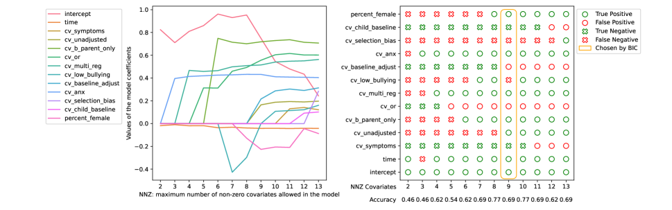
Figure 6: Validation of Random Feature Selection for Bullying Data from GBD 2020. Left panel shows coefficient paths across numbers of nonzero covariates allowed in the model using the $\ell_{0}$ regularizer. Right panel shows evaluation of each choice, evaluated against expert knowledge from past datasets. The algorithm picks seven historically significant covariates and two historically insignificant, for the model selected using the BIC criteria. See the Appendix B.2 for covariates description and assessment of significance.

In this section we validate the SR3-empowered $\ell_{0}$-regularized mixed-effect model ($R(x)=\delta_{\|x\|_{0}\leq k}$ from Table 1) by using it to identify the most important covariates in real data on relative risk of anxiety and depressive disorders depending on the exposure to bullying in young age. This research has been a part of Global Burden of Diseases study for the last several years. The end goal is to estimate the burden (DALYs) of major depressive disorder (MDD) and anxiety disorders that are caused by bullying. For this risk factor, the exposure is primarily concentrated in childhood and adolescents, but the risk for MDD and anxiety disorders is anticipated to continue well into adulthood. This elevated risk is, however, expected to decrease with time as other risk factors come into play in adulthood (unemployment, relationship issues, etc.). To accommodate this, the research team uses the models which estimate the relative risk (RR) of MDD and anxiety disorders among persons exposed to bullying depending on how many years it has been since the first exposure. Studies informing the model were sourced from a systematic review and consist of longitudinal cohort studies. They measure exposure to bullying at baseline, and then follow up years later and assess them for MDD or anxiety disorders. The detailed description of the covariates can be found in Appendix B.2.

The feature selection process is illustrated on Figures 4 and 6. Here, the BIC criterion from Jones (2011) was used to make a choice on $k$ (see the plot on the first row, column two on Figure 4). We see that there is a minimum around $k=4$, although the minimum is shallow so $k=5$ can also be considered. For the $k=4$ case, the selected covariates (intercept, time, cv_threshold_bullying, cv_b_parent_only) are known as important and were used in the analysis in previous years of GBD. For the $k=5$ case, the algorithm also selects cv_or and cv_child_baseline, which were not used before.

4.3 Software Implementation

In order to ensure reproducibility of our research, all developed algorithms have been implemented as a part of pysr3 library. This library implements functionality for fitting linear mixed models and selecting covariates. The user interface was designed to be fully compliant with the standards of sklearn library to minimize learning time.

5 Discussion

In this paper, we developed and implemented a first-order variable selection framework for LMEs that handles convex and nonconvex regularizers. We also showed that MSR3 relaxation, a regularizer-agnostic transformation of the likelihood, improves the covariates selection accuracy of a wide group of popular sparsity-promoting regularizers. The fact that relaxation improves accuracy, rather than just serving as a means to solve the original problem, is a very interesting result that can be studied in future work.

Since the LME relaxation does not have a closed form, we used an interior method to evaluate the requisite value function. We also developed a more efficient version of the algorithm (MSR3-Fast) that interleaved interior point iterations with updates of the auxiliary variables, and this method was chosen for the open source library pysr3 that we provided. Numerical experiments on synthetic data showed that the MSR3 approach for variable selection extends regions of hyper-parameter values where the highest accuracy is achieved, making it easier for information criteria to select the best model. The variable selection library for the accelerated method MSR3-Fast is much faster than currently available software, and allows the MSR3 approach to be easily applied to a range of regularizers that have prox operators available.

The main analytic limitations of the proposed method stem from a lack of an analytical representation of the value function in the MSR3 relaxation for LMEs. In contrast to linear regression settings, where the CG method can be efficiently used to evaluate the value function Baraldi et al. (2019), the nonlinear optimization problem required for LMEs is more difficult. Using Hessian information makes each iteration computationally efficient but limits the problem size. At the same time, switching to first-order methods for the inner problem inside the relaxation may be prohibitively slow. One way to mitigate the problem would be to build more efficient upper-bound models for the value function that can be evaluated effectively.

The suggested methodology can be expanded to a wider class of models. In particular, one can extend MSR3 to the setting of non-linear mixed-effect models or generalized linear mixed models, which are known to be challenging setups for covariate selection tasks. Both of these problem classes face similar challenges with respect to optimization strategies for highly nonlinear objective functions that arise when we consider marginal likelihoods in these settings. On the other hand, the SR3 strategy would allow any fast solver to be extended to variable selection task through the relaxation reformulation, analogously to what was done here for LMEs.

Appendix A Additional derivations

A.1 Derivatives of Marginalized Log-likelihood for Linear Mixed Models

For conciseness, let us define the mismatch $\xi_{i}=Y_{i}-X_{i}\beta$. The loss function 3 takes the form

$$\begin{split}\operatorname{\mathcal{L}}(\gamma)=\sum_{i=1}^{m}\frac{1}{2}\xi_{i}^{T}(\Omega_{i}(\gamma))^{-1}\xi_{i}+\frac{1}{2}\log\det(\Omega_{i}(\gamma)).\end{split}$$ (27)

The derivative of the objective w.r.t $\gamma_{j}$, the $j$’th diagonal element of the matrix $\Gamma$ is

$$\begin{split}\frac{\partial\xi_{i}^{T}\Omega_{i}^{-1}\xi_{i}}{\partial\Gamma_{jj}}&=\operatorname{Tr}\left[\left(\frac{\partial\xi_{i}^{T}\Omega_{i}^{-1}\xi_{i}}{\partial\Omega_{i}}\right)\frac{\partial\Omega}{\partial\Gamma_{jj}}\right]=\operatorname{Tr}\left[\left(-\Omega_{i}^{-1}\xi_{i}\xi_{i}^{T}\Omega_{i}^{-1}\right)^{T}Z_{i}\frac{\partial\Gamma}{\partial\Gamma_{jj}}Z_{i}^{T}\right]\end{split}$$ (28)

where $\frac{\partial\Gamma}{\partial\Gamma_{jj}}$ is a single-entry matrix $J^{jj}$ with $jj$’th element is equal to 1 and zeroes elsewhere. Plugging in the value and making a circular swap, we get Substituting this back we get

$$\begin{split}\frac{\partial\xi_{i}^{T}\Omega_{i}^{-1}\xi_{i}}{\partial\Gamma_{jj}}=\operatorname{Tr}\left[-{Z^{j}_{i}}^{T}\Omega_{i}^{-1}\xi_{i}\xi_{i}^{T}\Omega_{i}^{-1}Z^{j}_{i}\right]=-({Z_{i}^{j}}^{T}\Omega_{i}^{-1}\xi_{i})^{2}\end{split}$$ (29)

Similarly,

$$\begin{split}\frac{\partial\log\det\Omega_{i}}{\partial\Gamma_{jj}}=\operatorname{Tr}\left[\left(\frac{\partial\log\det\Omega_{i}}{\partial\Omega_{i}}\right)\frac{\partial\Omega_{i}}{\partial\Gamma_{jj}}\right]=\operatorname{Tr}\left[\Omega_{i}^{-1}Z_{i}^{j}{Z_{i}^{j}}^{T}\right]={Z_{i}^{j}}^{T}\Omega_{i}^{-1}Z_{i}^{j}\end{split}$$ (30)

Using symmetry of $\Omega_{i}$, we have

$$\begin{split}\nabla_{\gamma}\operatorname{\mathcal{L}}(\beta,\gamma)=\sum_{i=1}^{m}\mathrm{diag}\left(({Z_{i}}^{T}\Omega_{i}^{-1}Z_{i})\right)-({Z_{i}}^{T}\Omega_{i}^{-1}\xi_{i})^{\circ 2}\end{split}$$ (31)

where $\circ$ denotes the Hadamard (element-wise) product and $\mathrm{diag}\left(\cdot\right)$ takes a square matrix to its diagonal. Using the Cholesky decomposition $\Omega_{i}=L_{i}L_{i}^{T}$ we can calculate (31) using only one triangular matrix inversion:

$$\begin{split}\nabla_{\gamma}\operatorname{\mathcal{L}}(\beta,\gamma)=\sum_{i=1}^{m}\left[\sum_{\text{rows}}\left(L_{i}^{-1}Z_{i}\right)^{\circ 2}-[(L_{i}^{-1}Z_{i})^{T}(L_{i}^{-1}\xi_{i})]^{\circ 2}\right]\end{split}$$ (32)

Notice, that the loss function (3) and the optimal $\beta$ can also be effectively computed using Cholesky:

$$\begin{split}\operatorname{\mathcal{L}}(\gamma)=\sum_{i=1}^{m}\frac{1}{2}\xi_{i}^{T}(\Omega_{i}(\gamma))^{-1}\xi_{i}+\frac{1}{2}\log\det(\Omega_{i}(\gamma))=\sum_{i=1}^{m}\frac{1}{2}\ \|L_{i}^{-1}\xi_{i}\|^{2}-\sum_{j=1}^{k}\log{[L^{-1}_{i}]}_{jj}\end{split}$$ (33)

$$\begin{split}\beta_{k+1}&=\operatorname*{\mathrm{argmin}}_{\beta}\operatorname{\mathcal{L}}(\beta,\gamma_{k})=\left(\sum_{i=1}^{m}X_{i}^{T}\Omega_{i}^{-1}X_{i}\right)^{-1}\sum_{i=1}^{m}X_{i}^{T}\Omega_{i}^{-1}y_{i}=\\ &=\left(\sum_{i=1}^{m}(L_{i}^{-1}X_{i})^{T}L_{i}^{-1}X_{i}\right)^{-1}\sum_{i=1}^{m}(L_{i}^{-1}X_{i})^{T}L_{i}^{-1}y_{i}\end{split}$$ (34)

The Hessian w.r.t. $\gamma$ is derived below:

$$\begin{split}\frac{\partial^{2}\operatorname{\mathcal{L}}(\beta,\gamma)}{\partial\gamma_{j}^{2}}&=\sum_{i=1}^{m}-2({Z_{i}^{j}}^{T}\Omega_{i}^{-1}\xi_{i})\operatorname{Tr}\left[\frac{\partial{Z_{i}^{j}}^{T}\Omega_{i}^{-1}\xi_{i}}{\partial\Omega_{i}}\frac{\partial\Omega_{i}}{\partial\Gamma_{jj}}\right]+\operatorname{Tr}\left[\frac{\partial{Z_{i}^{j}}^{T}\Omega_{i}^{-1}Z_{i}^{j}}{\partial\Omega_{i}}\frac{\partial\Omega_{i}}{\partial\Gamma_{jj}}\right]=\\ &=\sum_{i=1}^{m}2({Z_{i}^{j}}^{T}\Omega_{i}^{-1}\xi_{i})\operatorname{Tr}\left[\Omega_{i}^{-1}Z_{i}^{j}{\xi_{i}}^{T}\Omega_{i}^{-1}Z_{i}^{j}{Z_{i}^{j}}^{T}\right]-({Z_{i}^{j}}^{T}\Omega_{i}^{-1}Z_{i}^{j})^{2}=\\ &=\sum_{i=1}^{m}2({Z_{i}^{j}}^{T}\Omega_{i}^{-1}\xi_{i})({Z_{i}^{j}}^{T}\Omega_{i}^{-1}Z_{i}^{j})({\xi_{i}}^{T}\Omega_{i}^{-1}Z_{i}^{j})-({Z_{i}^{j}}^{T}\Omega_{i}^{-1}Z_{i}^{j})^{2}\end{split}$$ (35)

$$\begin{split}\frac{\partial^{2}\operatorname{\mathcal{L}}(\beta,\gamma)}{\partial\gamma_{j}\partial\gamma_{k}}&=\sum_{i=1}^{m}-2({Z_{i}^{j}}^{T}\Omega_{i}^{-1}\xi_{i})\operatorname{Tr}\left[\frac{\partial{Z_{i}^{j}}^{T}\Omega_{i}^{-1}\xi_{i}}{\partial\Omega_{i}}\frac{\partial\Omega_{i}}{\partial\Gamma_{kk}}\right]+\operatorname{Tr}\left[\frac{\partial{Z_{i}^{j}}^{T}\Omega_{i}^{-1}Z_{i}^{j}}{\partial\Omega_{i}}\frac{\partial\Omega_{i}}{\partial\Gamma_{kk}}\right]=\\ &=\sum_{i=1}^{m}2({Z_{i}^{j}}^{T}\Omega_{i}^{-1}\xi_{i})\operatorname{Tr}\left[\Omega_{i}^{-1}Z_{i}^{j}{\xi_{i}}^{T}\Omega_{i}^{-1}Z_{i}^{k}{Z_{i}^{k}}^{T}\right]-({Z_{i}^{j}}^{T}\Omega_{i}^{-1}Z_{i}^{k})^{2}=\\ &=\sum_{i=1}^{m}2(\xi_{i}^{T}\Omega_{i}^{-1}{Z_{i}^{j}})({Z_{i}^{j}}^{T}\Omega_{i}^{-1}Z_{i}^{k})({Z_{i}^{k}}^{T}\Omega_{i}^{-1}{\xi_{i}})-({Z_{i}^{j}}^{T}\Omega_{i}^{-1}Z_{i}^{k})^{2}\end{split}$$ (36)

$$\begin{split}\nabla^{2}_{\gamma}\operatorname{\mathcal{L}}(\beta,\gamma)=\frac{1}{2}\sum_{i=1}^{m}-(Z_{i}^{T}\Omega_{i}^{-1}Z_{i})^{\circ 2}+2\mathrm{Diag}\left(Z_{i}^{T}\Omega_{i}^{-1}\xi_{i}\right)(Z_{i}^{T}\Omega^{-1}Z_{i})\mathrm{Diag}\left(\xi_{i}^{T}\Omega^{-1}Z_{i}\right)=\\ =\frac{1}{2}\sum_{i=1}^{m}-(Z_{i}^{T}\Omega_{i}^{-1}Z_{i})^{\circ 2}+2(Z_{i}^{T}\Omega_{i}^{-1}\xi_{i})(\xi_{i}^{T}\Omega^{-1}Z_{i})^{T}\circ(Z_{i}^{T}\Omega^{-1}Z_{i})\end{split}$$ (37)

A.2 Derivation of Selected Proximal Operators from Table 1

SCAD

For a scalar variable $x\in\operatorname{\mathbb{R}}$, SCAD-regularizer is defined as

$$\begin{split}r(x)=\begin{cases}\sigma|x|,&|x|\leq\sigma\\ \frac{-x^{2}+2\rho\sigma|x|-\sigma^{2}}{2(\rho-1)},&\sigma<|x|<\rho\sigma\\ \frac{\sigma^{2}(\rho+1)}{2},&|x|>\rho\sigma\end{cases}\end{split}$$ (38)

To evaluate the ${\mathrm{prox}}_{\alpha r}$ operator we need to solve the following minimization problem:

$$\begin{split}\min_{x}r(x)+\frac{1}{2\alpha}(x-z)^{2}\end{split}$$ (39)

For $\alpha=1$, the solution was derived by Fan (1997). Here we extend it for an arbitrary $\alpha$. To identify the set of stationary points $\{x^{*}\}$ of a non-smooth function $f(x)$, we the optimality condition

$$\begin{split}0\in\partial_{x}f(x^{*})\end{split}$$ (40)

where $\partial_{x}f(x)$ denotes a sub-differential set of $f$ at the point $x$. For the prox problem, we get

$$\begin{split}0\in\frac{1}{\alpha}(x^{*}-z)+\partial r(x)_{x=x^{*}}\end{split}$$ (41)

Since $r(x)$ is piece-wise defined the precise value of $\partial r(x)_{x=x^{*}}$ will depend on $x^{*}$:

1. Let $0<x^{*}\leq\sigma$, then we have $\partial r(x)_{x=x^{*}}=\{x^{*}\}$ and so

   $$\begin{split}x=z-\sigma\alpha,\quad z\in[\sigma\alpha,\sigma+\sigma\alpha]\end{split}$$ (42)

2. Let $-\sigma\alpha\leq x^{*}<0$, then we have $\partial r(x)_{x=x^{*}}=\{-x^{*}\}$ and so

   $$\begin{split}x=z+\sigma\alpha,\quad z\in[-\sigma-\sigma\alpha,-\sigma\alpha]\end{split}$$ (43)

3. Let $x^{*}=0$, then $\partial r(x)_{x=x^{*}}=[-1,1]$, which yields

   $$\begin{split}\frac{1}{\alpha}(x^{*}-z)\in-\sigma[-1,1]\quad\Rightarrow\quad z\in[-\sigma\alpha,\sigma\alpha]\end{split}$$ (44)

4. Let $\sigma<x^{*}<\rho\sigma$, then $r(x)_{x=x^{*}}=\frac{-{x^{*}}^{2}+2\rho\sigma x^{*}-\sigma^{2}}{2(\rho-1)}$, which gives us

   $$\begin{split}\frac{1}{\alpha}(x^{*}-z)=\frac{x^{*}-\rho\sigma}{\rho-1}\end{split}$$ (45)

   To ensure that the stationary point is indeed a minimizer, we need to ensure that

   $$\begin{split}\frac{1}{\alpha}-\frac{1}{\rho-1}>0\quad\Rightarrow\quad\alpha<\rho-1.\end{split}$$ (46)

   Rearranging the terms to express $x^{*}$ as a function of $z$ we get

   $$\begin{split}x^{*}=\frac{(\rho-1)z-\lambda\rho\sigma}{\rho-1-\alpha}\quad\Rightarrow\quad z\in[\sigma+\alpha\sigma,\rho\sigma]\end{split}$$ (47)

5. Let $-\rho\sigma<x^{*}<-\sigma$, then, similarly to the previous case, we get

   $$\begin{split}\frac{1}{\alpha}(x^{*}-z)=\frac{x^{*}+\rho\sigma}{\rho-1}\end{split}$$ (48)

   Rearranging the terms to express $x$ in terms of $z$ we get:

   $$\begin{split}x^{*}=\frac{(\rho-1)z+\lambda\rho\sigma}{\rho-1-\alpha}\quad\Rightarrow\quad z\in[-\sigma-\alpha\sigma,-\sigma]\end{split}$$ (49)

6. Finally, when $|x^{*}|\geq\sigma\rho$ we have $\partial r(x)_{x=x^{*}}=\{0\}$ and so

   $$\begin{split}x^{*}=z,\quad|z|\geq\sigma\rho\end{split}$$ (50)

   Bundling all six cases together, we have

   $$\begin{split}{\mathrm{prox}}_{\alpha r}(z)=\begin{cases}\operatorname*{\mathrm{sign}}(z)(|z|-\sigma\alpha)_{+},&|z|\leq\sigma(1+\alpha)\\ \frac{(\rho-1)z-\operatorname*{\mathrm{sign}}(z)\rho\sigma\alpha}{\rho-1-\alpha},&\sigma(1+\alpha)<|z|\leq\max(\rho,1+\alpha)\sigma\\ z,&|z|>\max(\rho,1+\alpha)\sigma\end{cases}\end{split}$$ (51)

   The middle branch is active only when $\rho>1+\alpha$. One special case of this is when $\alpha=1$, and then (51) recovers the classic result by Fan and Li (2001).

   To get ${\mathrm{prox}}_{\alpha r+\delta_{\operatorname{\mathbb{R}}_{+}}}(z)$ from ${\mathrm{prox}}_{\alpha r}(z)$ we only need to notice that (1) the minimizer $x^{*}$ of

   $$\begin{split}\min_{x}r(x)+\delta_{\operatorname{\mathbb{R}}_{+}}+\frac{1}{\alpha}(x-z)^{2}\end{split}$$ (52)

   can never be negative, and that (2) when the minimizer $x^{*}$ is exactly zero we get:

   $$\begin{split}\frac{1}{\alpha}(x^{*}-z)\in-\partial(r(x)|_{x=x^{*}}+\delta_{\operatorname{\mathbb{R}}_{+}}(x)|_{x=x^{*}})\quad\Rightarrow\quad z\in[-\infty,\sigma\alpha]\end{split}$$ (53)

A-LASSO

A-LASSO regularizer is defined as

$$\begin{split}r(x)=w|x|\end{split}$$ (54)

where $w=1/|\hat{x}|$ with $\hat{x}$ the solution of a non-regularized problem (Zou (2006)). The derivation of the proximal operator of A-LASSO nearly matches the steps 1, 2, and 3 that of SCAD above. We wish to evaluate

$$\begin{split}\min_{x}w|x|+\frac{1}{2\alpha}(x-z)^{2}\end{split}$$ (55)

as a function of $z$. The sub-differential optimality criterion yields

$$\begin{split}0\in\frac{1}{\alpha}(x^{*}-z)+w\partial|x|\end{split}$$ (56)

1. Let $0<x^{*}$, then we have $\partial r(x)_{x=x^{*}}=\{x^{*}\}$ and so

   $$\begin{split}x^{*}=z-\alpha w,\quad z>\alpha w\end{split}$$ (57)

2. Let $x^{*}<0$, then we have $\partial r(x)_{x=x^{*}}=\{-x^{*}\}$ and so

   $$\begin{split}x^{*}=z+\alpha w,\quad z<-\alpha w\end{split}$$ (58)

3. Let $x^{*}=0$, then $\partial r(x)_{x=x^{*}}=[-1,1]$, which yields

   $$\begin{split}\frac{1}{\alpha}(x^{*}-z)\in[-w,w]\quad\Rightarrow\quad z\in[-\alpha w,\alpha w]\end{split}$$ (59)

Combining all cases together we get

$$\begin{split}{\mathrm{prox}}_{\alpha r}(z)=\operatorname*{\mathrm{sign}}(z)(|z|-\alpha w)_{+}\end{split}$$ (60)

Finally, ${\mathrm{prox}}_{\alpha r+\delta_{\operatorname{\mathbb{R}}}}(z)$ can be derived by noticing that, in this case, (1) $x^{*}\geq 0$, and (2) when $x^{*}=0$ the sub-differential changes due to the presence of the delta-function:

$$\begin{split}x^{*}=0\implies\frac{1}{\alpha}(x^{*}-z)\in-([-\alpha w,\alpha w]+[-\infty,0])=[-\alpha w,+\infty]\end{split}$$ (61)

which gives us the condition

$$\begin{split}x^{*}=z,\quad z\in[-\infty,\alpha w].\end{split}$$ (62)

LASSO

LASSO is a particular case of A-LASSO above when $w=1$.

$\ell_{0}$-regularizer

Comparing to its counterparts above, the regularizer $R(x)=\delta_{\|x\|\leq k}(x)$ is non-separable. However, the proximal operator of it can still be evaluated analytically:

$$\begin{split}\left[{\mathrm{prox}}_{\alpha R}(z)\right]_{i}=\left[\operatorname*{\mathrm{argmin}}_{\|x\|\leq k}\frac{1}{2\alpha}\|x-z\|^{2}\right]_{i}=\begin{cases}z_{i},&i\in\operatorname{\mathcal{I}}_{k}\\ 0,&\text{ otherwise}\end{cases}\end{split}$$ (63)

where $\operatorname{\mathcal{I}}_{k}$ is a set of $k$ largest in their absolute value coordinates of $z$. To get ${\mathrm{prox}}_{\alpha R+\delta_{\operatorname{\mathbb{R}}_{+}}}$ we replace $\operatorname{\mathcal{I}}_{k}$ with a set of $k$ largest positive coordinates of $z$, and set the rest of the coordinates to $0$.

A.3 Lipschitz-constant for Likelihood of a Linear Mixed-Effects Model

Recall that a function $\operatorname{\mathcal{L}}(x)$ is called L-Lipschitz smooth when

$$\begin{split}\|\nabla\operatorname{\mathcal{L}}(x)-\nabla\operatorname{\mathcal{L}}(y)\|_{2}\leq L\|x-y\|_{2}\end{split}$$ (64)

To find the Lipschitz-constant of the function $\operatorname{\mathcal{L}}_{ML}$ (3) we will use the fact that $\operatorname{\mathcal{L}}(x)$ is L-Lipschitz if and only if $\|\nabla^{2}\operatorname{\mathcal{L}}(x)\|\leq L$ for any $x$. Hence, to upper-bound L we need to upper-bound the norms of Hessians. Assume that $\|y_{i}-X_{i}\beta\|\leq\eta$ where $\eta>0$. We get

$$\begin{split}\left\|\nabla^{2}\operatorname{\mathcal{L}}(x)\right\|_{2}&=\left\|\begin{bmatrix}\nabla^{2}_{\beta\beta}\operatorname{\mathcal{L}}(\beta,\gamma)&\nabla^{2}_{\beta\gamma}\operatorname{\mathcal{L}}(\beta,\gamma)\\ \nabla^{2}_{\gamma\beta}\operatorname{\mathcal{L}}(\beta,\gamma)&\nabla^{2}_{\gamma\gamma}\operatorname{\mathcal{L}}(\beta,\gamma)\end{bmatrix}\right\|\leq\sum_{i=1}^{m}\left\|\begin{bmatrix}\frac{\|X_{i}\|_{2}^{2}}{\|\Lambda_{i}\|_{2}}&\frac{\eta\|X_{i}\|_{2}\|Z_{i}\|^{2}_{2}}{\|\Lambda_{i}\|^{2}}\\ \frac{\eta\|X_{i}\|_{2}\|Z_{i}\|^{2}_{2}}{\|\Lambda_{i}\|^{2}}&\frac{\eta\|Z_{i}\|_{2}^{4}}{\|\Lambda_{i}\|_{2}^{3}}\end{bmatrix}\right\|\\ &\leq\sum_{i=1}^{m}\max\left(\frac{\|X_{i}\|_{2}^{2}}{\|\Lambda_{i}\|_{2}},\frac{\eta\|X_{i}\|_{2}\|Z_{i}\|^{2}_{2}}{\|\Lambda_{i}\|^{2}},\frac{\eta\|X_{i}\|_{2}\|Z_{i}\|^{2}_{2}}{\|\Lambda_{i}\|^{2}},\frac{\eta\|Z_{i}\|_{2}^{4}}{\|\Lambda_{i}\|_{2}^{3}}\right)=L\end{split}$$ (65)

Appendix B Description of Datasets and Experiments

Table 4 provides a more detailed overview of the relative performance of the algorithms from the Table 2.

B.1 Detailed Results from Simulation from Table 2

	Regularizer	L0	L1	ALASSO	SCAD
Model	Metric
PGD	Accuracy	89 (75-95)	73 (68-82)	88 (72-98)	71 (62-78)
	FE Accuracy	88 (70-95)	56 (45-70)	84 (65-100)	53 (45-65)
	RE Accuracy	90 (75-100)	91 (80-100)	92 (80-100)	89 (75-100)
	F1	88 (74-95)	77 (71-83)	88 (74-97)	75 (68-80)
	FE F1	87 (72-95)	67 (62-75)	85 (70-100)	66 (62-72)
	RE F1	89 (74-100)	91 (78-100)	91 (78-100)	88 (74-100)
	Time	25.73 (17.21-38.69)	23.37 (16.35-32.26)	20.24 (14.12-28.09)	48.50 (30.66-79.67)
	Iterations	29662 (20985-43234)	31693 (22361-45603)	28912 (20915-39210)	41724 (26911-69881)
MSR3	Accuracy	92 (75-98)	88 (65-100)	91 (75-100)	92 (75-100)
	FE Accuracy	92 (70-100)	84 (50-100)	90 (70-100)	93 (75-100)
	RE Accuracy	92 (80-100)	91 (75-100)	92 (75-100)	90 (75-100)
	F1	92 (76-97)	88 (71-100)	91 (74-100)	91 (77-100)
	FE F1	92 (75-100)	87 (64-100)	91 (75-100)	94 (76-100)
	RE F1	91 (78-100)	90 (74-100)	91 (74-100)	89 (71-100)
	Time	0.08 (0.06-0.11)	0.08 (0.06-0.11)	0.07 (0.06-0.09)	0.10 (0.07-0.13)
	Iterations	34 (28-43)	35 (27-50)	33 (27-39)	44 (30-59)

Table 4: Comparison of performance of algorithms

B.2 GBD Bullying Data

The author acknowledges his colleague and collaborator Damian Santomauro for providing the dataset, the description of its covariates, and the expert assessment of their historical importance in different rounds of GBD study below.

1. cv_symptoms

   • 0 = study assesses participants for MDD or anxiety disorders via a diagnostic interview to determine whether they have a diagnosis.

   • 1 = study uses a symptom scale (e.g., Beck Depression Inventory) and uses an established cut-off on that scale to determine caseness.

   • Has not been significant in the past.

2. cv_unadjusted

   • 0 = RR is adjusted for potential confounders (e.g., SES, etc.)

   • 1 = RR is not adjusted for potential confounders

   • Has been significant in the past.

3. cv_b_parent_only

   • 0 = Child is involved in reporting their own exposure to bullying.

   • 1 = Only parent is involved in reporting the child’s exposure to bullying

   • Has recently been significant.

4. cv_or

   • 0 = estimate is a RR

   • 1 = estimate is an odds ratio (OR)

   • ORs are always larger than RRs; covariate may not be significant.

5. cv_multi_reg

   • 0 = RR is the ratio of the rate of the outcome in persons exposed vs all persons unexposed (including persons exposed to low-threshold bullying victimization)

   • 1 = RRs are estimated via a logistic regression where exposure represented by 3 categories: 1) No exposure, 2) Occasional exposure, 3) Frequent exposure. The RR for occasional exposure will exclude participants with frequent exposure, and the RR for frequent exposure will exclude participants with occasional exposure.

   • Is expected to be significant.

6. cv_low_threshold_bullying

   • 0 = uses a ‘frequent’ exposure threshold for classing someone as exposed to bullying.

   • 1 = uses an ‘occasional’ exposure threshold for classing someone as exposed to bullying.

   • Has been significant in the past.

7. cv_anx

   • 0 = estimate represents risk for MDD

   • 1 = estimate represents risk for anxiety disorders

8. cv_selection_bias

   • 0 = < 15% attrition at followup

   • 1 = $\geqslant$ 15% attrition at followup

   • Has been significant in the past.

9. Percent_female

   • Indicates % of sample in estimate that are female.

10. cv_child_baseline

    • Indicates whether mid-age of sample is is above or below 13.

    • Has not been significant in the past.

References

- Attouch et al. (2013) Attouch, H., J. Bolte, and B. F. Svaiter (2013). Convergence of descent methods for semi-algebraic and tame problems: proximal algorithms, forward–backward splitting, and regularized gauss–seidel methods. Mathematical Programming 137(1), 91–129.
- Baraldi et al. (2019) Baraldi, R., R. Kumar, and A. Aravkin (2019, nov). Basis Pursuit Denoise With Nonsmooth Constraints. IEEE Transactions on Signal Processing 67(22), 5811–5823.
- Beck (2017) Beck, A. (2017). First-Order Methods in Optimization. MOS-SIAM Series on Optimization. SIAM.
- Bondell et al. (2010) Bondell, H. D., A. Krishna, and S. K. Ghosh (2010, dec). Joint Variable Selection for Fixed and Random Effects in Linear Mixed-Effects Models. Biometrics 66(4), 1069–1077.
- Buscemi and Plaia (2019) Buscemi, S. and A. Plaia (2019). Model selection in linear mixed-effect models. AStA Advances in Statistical Analysis.
- Chen et al. (2015) Chen, F., Z. Li, L. Shi, and L. Zhu (2015). Inference for mixed models of anova type with high-dimensional data. Journal of Multivariate Analysis 133, 382–401.
- Chen and Dunson (2003) Chen, Z. and D. B. Dunson (2003, dec). Random Effects Selection in Linear Mixed Models. Biometrics 59(4), 762–769.
- DerSimonian and Laird (1986) DerSimonian, R. and N. Laird (1986). Meta-analysis in clinical trials. Controlled clinical trials 7(3), 177–188.
- Fan (1997) Fan, J. (1997). Comments on “wavelets in statistics: A review” by a. antoniadis. Journal of the Italian Statistical Society 6(2), 131.
- Fan and Li (2001) Fan, J. and R. Li (2001, dec). Variable Selection via Nonconcave Penalized Likelihood and its Oracle Properties. Journal of the American Statistical Association 96(456), 1348–1360.
- Fan and Li (2012) Fan, Y. and R. Li (2012, aug). Variable selection in linear mixed effects models. The Annals of Statistics 40(4), 2043–2068.
- Fan et al. (2014) Fan, Y., G. Qin, and Z. Y. Zhu (2014). Robust variable selection in linear mixed models. Communications in Statistics-Theory and Methods 43(21), 4566–4581.
- Friedman et al. (2010) Friedman, J., T. Hastie, and R. Tibshirani (2010). Regularization paths for generalized linear models via coordinate descent. Journal of Statistical Software 33(1), 1–22.
- Ghosh and Thoresen (2018) Ghosh, A. and M. Thoresen (2018). Non-concave penalization in linear mixed-effect models and regularized selection of fixed effects. AStA Advances in Statistical Analysis 102(2), 179–210.
- Groll and Tutz (2014) Groll, A. and G. Tutz (2014). Variable selection for generalized linear mixed models by l 1-penalized estimation. Statistics and Computing 24(2), 137–154.
- Ibrahim et al. (2011a) Ibrahim, J. G., H. Zhu, R. I. Garcia, and R. Guo (2011a). Fixed and random effects selection in mixed effects models. Biometrics 67(2), 495–503.
- Ibrahim et al. (2011b) Ibrahim, J. G., H. Zhu, R. I. Garcia, and R. Guo (2011b, jun). Fixed and Random Effects Selection in Mixed Effects Models. Biometrics 67(2), 495–503.
- Jiang et al. (2008) Jiang, J., J. S. Rao, Z. Gu, and T. Nguyen (2008). Fence methods for mixed model selection. The Annals of Statistics 36(4), 1669–1692.
- Jones (2011) Jones, R. H. (2011, nov). Bayesian information criterion for longitudinal and clustered data. Statistics in Medicine 30(25), 3050–3056.
- Kojima et al. (1991) Kojima, M., N. Megiddo, T. Noma, and A. Yoshise (1991, jul). A unified approach to interior point algorithms for linear complementarity problems: A summary. Operations Research Letters 10(5), 247–254.
- Lan (2006) Lan, L. (2006). Variable Selection in Linear Mixed Model for Longitudinal Data. PhD thesis.
- Lin et al. (2013a) Lin, B., Z. Pang, and J. Jiang (2013a). Fixed and random effects selection by REML and pathwise coordinate optimization. Journal of Computational and Graphical Statistics 22(2), 341–355.
- Lin et al. (2013b) Lin, B., Z. Pang, and J. Jiang (2013b). Fixed and random effects selection by reml and pathwise coordinate optimization. Journal of Computational and Graphical Statistics 22(2), 341–355.
- Müller et al. (2013) Müller, S., J. L. Scealy, and A. H. Welsh (2013). Model selection in linear mixed models. Statistical Science 28(2), 135–167.
- Murray et al. (2020) Murray, C. J., A. Y. Aravkin, P. Zheng, C. Abbafati, K. M. Abbas, M. Abbasi-Kangevari, F. Abd-Allah, A. Abdelalim, M. Abdollahi, I. Abdollahpour, et al. (2020). Global burden of 87 risk factors in 204 countries and territories, 1990–2019: a systematic analysis for the global burden of disease study 2019. The Lancet 396(10258), 1223–1249.
- Nesterov and Nemirovskii (1994) Nesterov, Y. and A. Nemirovskii (1994, jan). Interior-Point Polynomial Algorithms in Convex Programming. Society for Industrial and Applied Mathematics.
- Nocedal and Wright (2006) Nocedal, J. and S. Wright (2006). Numerical optimization. Springer Science & Business Media.
- Pan and Shang (2018) Pan, J. and J. Shang (2018). A simultaneous variable selection methodology for linear mixed models. Journal of Statistical Computation and Simulation 88(17), 3323–3337.
- Patterson and Thompson (1971) Patterson, H. D. and R. Thompson (1971, dec). Recovery of Inter-Block Information when Block Sizes are Unequal. Biometrika 58(3), 545.
- Pinheiro and Bates (2006) Pinheiro, J. and D. Bates (2006). Mixed-effects models in S and S-PLUS. Springer science & business media.
- Pinheiro and Bates (2000) Pinheiro, J. C. and D. M. Bates (2000, sep). Mixed-Effects Models in Sand S-PLUS. Journal of the American Statistical Association 96(455), 1135–1136.
- Reiner et al. (2020) Reiner, R. C., R. M. Barber, J. K. Collins, P. Zheng, S. I. Hay, S. S. Lim, C. J. L. Murray, and IHME COVID-19 Forecasting Team (2020). Modeling covid-19 scenarios for the United States. Nature medicine.
- Rockafellar and Wets (2009) Rockafellar, R. T. and R. J.-B. Wets (2009). Variational analysis, Volume 317. Springer Science & Business Media.
- Schelldorfer et al. (2011) Schelldorfer, J., P. Bühlmann, and S. V. DE GEER (2011). Estimation for high-dimensional linear mixed-effects models using l1-penalization. Scandinavian Journal of Statistics 38(2), 197–214.
- Sholokhov (2022) Sholokhov, Burke, A. Z. (2022). A relaxation approach to feature selection for linear mixed effects models. In Preparation.
- Sugiura (1978) Sugiura, N. (1978, jan). Further analysts of the data by akaike’ s information criterion and the finite corrections. Communications in Statistics - Theory and Methods 7(1), 13–26.
- Tibshirani (1996a) Tibshirani, R. (1996a). Regression shrinkage and selection via the lasso. Journal of the Royal Statistical Society: Series B (Methodological) 58(1), 267–288.
- Tibshirani (1996b) Tibshirani, R. (1996b, jan). Regression Shrinkage and Selection Via the Lasso. Journal of the Royal Statistical Society: Series B (Methodological) 58(1), 267–288.
- Vaida and Blanchard (2005) Vaida, F. and S. Blanchard (2005, jun). Conditional Akaike information for mixed-effects models. Biometrika 92(2), 351–370.
- Wright (1997) Wright, S. J. (1997, jan). Primal-Dual Interior-Point Methods. Society for Industrial and Applied Mathematics.
- Xu et al. (2015) Xu, P., T. Wang, H. Zhu, and L. Zhu (2015). Double Penalized H-Likelihood for Selection of Fixed and Random Effects in Mixed Effects Models. Statistics in Biosciences 7(1), 108–128.
- Zheng et al. (2019) Zheng, P., T. Askham, S. L. Brunton, J. N. Kutz, and A. Y. Aravkin (2019). A Unified Framework for Sparse Relaxed Regularized Regression: SR3. IEEE Access 7, 1404–1423.
- Zheng et al. (2021) Zheng, P., R. Barber, R. J. Sorensen, C. J. Murray, and A. Y. Aravkin (2021). Trimmed constrained mixed effects models: formulations and algorithms. Journal of Computational and Graphical Statistics, 1–13.
- Zou (2006) Zou, H. (2006). The adaptive lasso and its oracle properties. Journal of the American Statistical Association 101(476), 1418–1429.
- Zuur et al. (2009) Zuur, A., E. N. Ieno, N. Walker, A. A. Saveliev, and G. M. Smith (2009). Mixed effects models and extensions in ecology with R. Springer Science & Business Media.