On the Accuracy of Three-dimensional Kinematic Distances

Abstract

Over the past decade, the BeSSeL Survey and the VERA project have measured trigonometric parallaxes to $\approx 250$ massive, young stars using VLBI techniques. These sources trace spiral arms over nearly half of the Milky Way. What is now needed are accurate distances to such stars which are well past the Galactic center. Here we analyze the potential for addressing this need by combining line-of-sight velocities and proper motions to yield 3D kinematic distance estimates. For sources within about 10 kpc of the Sun, significant systematic uncertainties can occur, and trigonometric parallaxes are generally superior. However, for sources well past the Galactic center, 3D kinematic distances are robust and more accurate than can usually be achieved by trigonometic parallaxes.

1 Introduction

Traditional kinematic distances for sources in the Galactic plane, estimated by comparing line-of-sight ($V_{\rm LSR}$) velocities with those expected from a model of Galactic rotation, while extensively used for decades, have significant limitations. For sources within the “Solar Circle” (ie, Galactocentric radii less than that of the Sun), a given $V_{\rm LSR}$ value occurs at two distances, and it is often difficult to discriminate between them. For Galactic longitudes within about $\pm 15{{}^{\circ}}$ of the Galactic center and anticenter, ${V_{\rm LSR}}$ values are near zero for most distances and, thus, kinematic distances have very large uncertainties. Also, near “tangent points” (where the Sun–Source–Galactic Center angle is $90{{}^{\circ}}$), small uncertainties in $V_{\rm LSR}$ lead to large errors in distance, since the gradient of $V_{\rm LSR}$ with distance vanishes. Finally, with only one component of a 3-dimenensional (3D) velocity vector, there is no consistency check on the accuracy of the assumption of circular Galactic orbits.

Sofue (2011) suggested using proper motions in addition to line-of-sight velocities to constrain the Galaxy’s rotation curve and, then, to estimate distances, emphasizing the complementary information available in two components of motion. Recently, Yamauchi et al. (2016) measured the proper motion in Galactic longitude of the source G007.47+0.06 ($-5.03\pm 0.07$ mas y^-1). They used this to obtain a 2-dimensional (2D) “kinematic distance” of $20\pm 2$ kpc, corresponding to 12 kpc past the Galactic center. Shortly thereafter, Sanna et al. (2017) reported a trigonometric parallax-distance of $20.4^{+2.8}_{-2.2}$ kpc for this source, supporting the Yamauchi et al.  estimate.

In this paper we expand on the 2D kinematic distance method by including proper motion in Galactic latitude to obtain full 3D kinematic distances as described in Section 2. We evaluate the accuracy of 3D kinematic distances by comparing them to large numbers of parallax measurements in Section 3. Next, we use simulations in Section 4 to quantify expected distance precision and accuracy in the presence of random non-circular motions. Then, in Section 5, we investigate sources of systematic error from inaccuracies in the assumed Galactic rotation curve and for anomalous motions seen in sources near the end of the Galactic bar. Finally, in Section 6, we summarize and comment on potential applications of 3D kinematic distances.

2 Estimating Distance with 3D Motions

3D kinematic distance estimates come from combining probability density as a function of distance for the line-of-sight velocity and the proper motion components in Galactic longitude and latitude. Assuming the measured values are Gaussianly distributed, the probability density function (PDF) for the line-of-sight velocity component is given by the following:

$${\rm Prob}_{v}(d|v,\sigma_{v},RC)\propto{1\over\sigma_{v}}e^{-\Delta v^{2}/2\sigma_{v}^{2}}~{}~{},$$

where $\Delta v$ is the measured value of the line-of-sight velocity component minus a value predicted by a rotation curve ($RC$), and $\sigma_{v}$ is the uncertainty in the measurement. For one component of proper motion (toward Galactic longitude or latitude) the PDF is given by:

$${\rm Prob}_{\mu}(d|\mu,\sigma_{\mu},RC)\propto{1\over\sigma_{\mu}}e^{-\Delta\mu^{2}/2\sigma_{\mu}^{2}}~{}~{},$$

where $\Delta\mu$ is the measured proper motion component minus the velocity predicted from the rotation curve divided by distance. For orbits within the Galactic plane, the expected Galactic latitude motion should be small. However, the PDF should be broader for nearby compared to distant sources, thereby providing some distance information.

We multiply the three component PDFs to yield a combined 3D likelihood function, from which we estimate a distance to the source from the location of peak of the function. Fig. 1 provides an example of the method for a simulated source toward longitude $15{{}^{\circ}}$ at 12 kpc distance and with 7 km s^-1 random noise added to each component of velocity. Plotted are PDFs vs distance for each of the three components of velocity, and the heavy black line is the combined 3D likelihood. Note that the 3D likelihood resolves distance ambiguities apparent in both the line-of-sight velocity and the longitude proper motion PDFs.

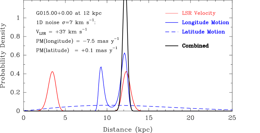
Figure 1: Simulated probability density functions (PDFs) for 3 components of velocity for a source at longitude $15^{\circ}$ at a distance of 12 kpc and with 7 km s^-1 noise added to each component (see listed $V_{\rm LSR}$ and proper motion (PM) values). The black likelihood function combines the 3 component PDFs (i.e.,  3D kinematic distance) and its peak and width provides an accurate and robust distance estimate and uncertainty.

We estimate distance from the peak of the combined 3D likelihood and assign a formal uncertainty from the half-width in distance between points at $e^{-0.5}$ about the peak. This formal uncertainty can underestimate a realistic error when the (unnormalized) 3D likelihood peak is low. This can happen, for example, when the line-of-sight velocity gives a distance that is in significant tension with that from the Galactic longitude motion, and the resulting 3D likelihood function can be too narrow to indicate uncertainty reliably. In order to deal with such cases, we calculate an alternative uncertainty as half the separation of the peaks of the line-of-sight velocity and Galactic longitude motion PDFs. We then report the maximum of this uncertainty and the formal uncertainty to arrive at a more conservative distance uncertainty.

3 Comparison of 3D Kinematic Distances with Parallaxes

Using the parallaxes and proper motions compiled by Reid et al. (2019) from the Bar and Spiral Structure Legacy (BeSSeL) Survey (bessel.vlbi-astrometry.org) and the VLBI Exploration of Radio Astrometry (VERA) project (www.miz.nao.ac.jp), the left panel of Fig. 2 shows a good correspondence between the parallax distances and the 3D kinematic distances. We note that 3D kinematic distances for sources nearby ($d\mathrel{\hbox{\raise 2.15277pt\hbox{$<$}\hbox to0.0pt{\hss\lower 2.15277pt\hbox{$\sim$}}}}8$ kpc) are slightly biased toward larger values compared to parallaxes. This occurs because astrophysical noise (eg, Virial motions of $\sim 7$ km s^-1) in the longitude and latitude directions leads to asymmetric PDFs when dividing by distance to convert to angular motion. As distance approaches zero, this effect is magnified. Fortunately, this bias decreases with increasing distance and does not significantly affect 3D kinematic distances for sources past the Galactic center (see Section 4 for results of simulations).

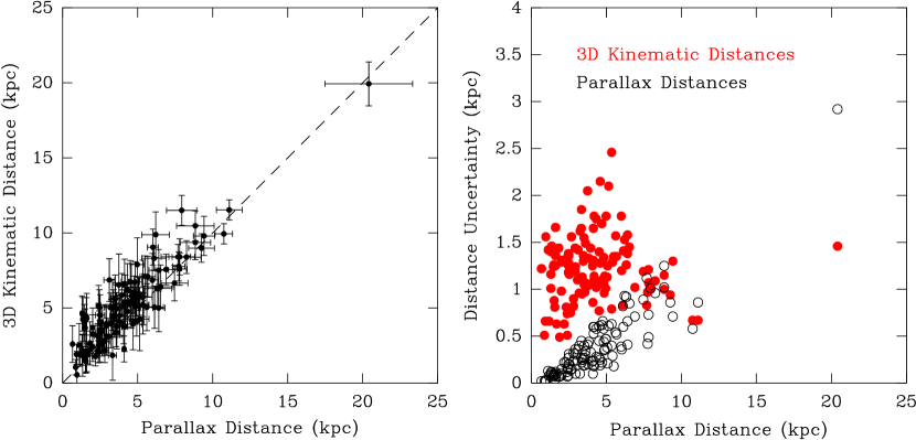
Figure 2: VLBI parallax and proper motion data from Reid et al. (2019) selecting only sources with fractional parallax uncertainty $<15$%. Left panel: Comparison of 3D kinematic vs parallax distances. Right panel: Uncertainties in the two methods vs distance. Note that 3D kinematic distance accuracy (red dots) matches and then surpases parallax accuracy (black circles) beyond about 8 kpc.

The right panel of Fig. 2 shows measurement uncertainty vs distance for the two methods. For nearby sources, 3D kinematic distances are considerably more uncertain than the parallax measurements. However, a given parallax uncertainty ($\sigma_{\pi}$) leads to increasing distance uncertainty with distance (since $\sigma_{d}=d^{2}\sigma_{\pi}$), and beyond $\approx 8$ kpc 3D kinematic distances tend to be more precise. The basic reason for this is that the longitude proper motion can be very large. For example, a source toward Galactic longitude 0.0 and well past the Galactic center will have an apparent longitude speed of $2\Theta_{0}\approx 470$ km/s, since for circular orbits the Sun and the source are moving in opposite directions with speeds of $\Theta_{0}$. Even if one misestimates a source’s motion by 20 km/s (eg, by measuring only one water maser spot occurring in an outflow of about that magnitude), that only corresponds to a 4% error. Also, errors of this magnitude in the assumed rotation curve will lead to similarly small distance errors. Except for sources within about 4 kpc of the Galactic center, the rotation curve of Reid et al. (2019), based on “gold standard” parallax distances and measured 3D motions, should be accurate to about $\pm 10$ km s^-1. We conclude that combining $V_{\rm LSR}$ and proper motion measurements can yield robust and precise distances for sources well past the Galactic center.

4 Effects of Random Non-Circular Motions

In this section, we investigate the accuracy of 3D kinematic distances by simulating observations of sources whose motions differ from an assumed rotation curve by the addition of random peculiar motions. Specifically, for a given Galactic longitude and distance from the Sun, we calculate the circular motion in the Galactic plane from the “universal rotation curve” formulation of Persic, Salucci & Stel (1996). This rotation curve is specified by only two parameters, and we adopt the $a2$ and $a3$ values from Reid et al. (2019) (from model A5) obtained by fitting parallax and proper motion data for 147 masers associated with very young ($<1$ My) and massive stars.

We add Gaussian random noise with $1\sigma$ dispersions, $\sigma_{v}$, of 7 or 20 km s^-1 to each of the three components of velocity. A one-dimensional dispersion of 7 km s^-1 corresponds to a full magnitude dispersion of 12 km s^-1, and is a good approximation of random Virial motions of young and massive stars within giant molecular clouds (Reid et al., 2009). A 20 km s^-1 dispersion is representative of much older stars and is shown to indicate the sensitivity of 3D kinematic distances to significantly larger dispersions. For each simulated source, we calculate its probability density functions and estimate distance as described in Section 2.

Fig. 3 displays the fractional distance error (ie, the difference between simulated and true distances divided by the true distance) as a function of the true distance for the two velocity dispersions. We calculate 10,000 independent trials for each true distance sampled every 0.5 kpc and connect the unweighted means of those trials. The representative error bars in Fig. 3 are standard deviations about the mean value and indicate the expected statistical ($1\sigma$) uncertainty in a single trial. The simulations reveal both statistical uncertainties and systematic biases in 3D kinematic distances.

Regarding statistical uncertainties, for magnitudes of Galactic longitude below $\approx 90{{}^{\circ}}$ (ie, in Galactic quadrants I and IV) and true distances $\mathrel{\hbox{\raise 2.15277pt\hbox{$>$}\hbox to0.0pt{\hss\lower 2.15277pt\hbox{$\sim$}}}}10$ kpc, fractional distance uncertainties are $\mathrel{\hbox{\raise 2.15277pt\hbox{$<$}\hbox to0.0pt{\hss\lower 2.15277pt\hbox{$\sim$}}}}10$%, corresponding to $\mathrel{\hbox{\raise 2.15277pt\hbox{$<$}\hbox to0.0pt{\hss\lower 2.15277pt\hbox{$\sim$}}}}\pm 1$ kpc at 10 kpc. For longitude magnitudes $>90{{}^{\circ}}$ (ie, quadrants II and III), statistical uncertainties start to grow, especially for the larger (20 km s^-1) random noise used in the simulations. This occurs because the sensitivity of both line-of-sight and longitude motions, which are proportional gradients in circular motion with distance, are low and random noise becomes relatively more important.

Systematic biases, owing to random peculiar motions, typically are less than several percent of distance at most Galactic longitudes for true distances $\mathrel{\hbox{\raise 2.15277pt\hbox{$>$}\hbox to0.0pt{\hss\lower 2.15277pt\hbox{$\sim$}}}}10$ kpc. For example, at a longitude of $30{{}^{\circ}}$ and a true distance of 12 kpc, random motions of 20 km s^-1 yield a bias in fractional distance of $<0.2$%, and this bias only grows to $1$% at a longitude of $120{{}^{\circ}}$. However, a clear inverse-distance bias towards larger estimated distances is seen for true distances $\mathrel{\hbox{\raise 2.15277pt\hbox{$<$}\hbox to0.0pt{\hss\lower 2.15277pt\hbox{$\sim$}}}}5$ kpc. This occurs because astrophysical noise (eg, Virial motions of $\sim 7$ km s^-1) in the longitude direction leads to an asymmetric PDF when dividing by distance to convert to angular motion. As distance approaches zero, this effect is magnifed. Fortunately, this bias is predictable, provided the velocity noise is known, and, in any event, it decreases with increasing distance and often becomes insignificant for distances $\mathrel{\hbox{\raise 2.15277pt\hbox{$>$}\hbox to0.0pt{\hss\lower 2.15277pt\hbox{$\sim$}}}}10$ kpc.

A second systematic problem is evident, for example, in the $5{{}^{\circ}}$ and $30{{}^{\circ}}$ longitude plots in Fig. 4 as a $\mathrel{\hbox{\raise 2.15277pt\hbox{$<$}\hbox to0.0pt{\hss\lower 2.15277pt\hbox{$\sim$}}}}10$% positive bias between true distances of 6 to 10 kpc for 20 km s^-1 added noise, and as a 30% positive bias in the $60{{}^{\circ}}$ longitude plot near 3.5 kpc for 7 km s^-1 added noise. These cases can also be identified by thier large standard deviations. They are caused by a combination of effects, including 1) near the tangent points (at 8.1, 7.1 and 4.1 kpc for longitudes of $5{{}^{\circ}}$, $30{{}^{\circ}}$, and $60{{}^{\circ}}$, respectively) the gradient in the line-of-sight velocity vanishes, and 2) a small number of trials can have a secondary probability peak at much larger distance which is slightly favored over the “primary” peak, owing to the addition of random motions. These cases can be recognized as problematic by examining the component PDFs in a manner similar to Fig. 1. However, here we have not attempted to remove such cases when presenting means and standard deviations from all trials.

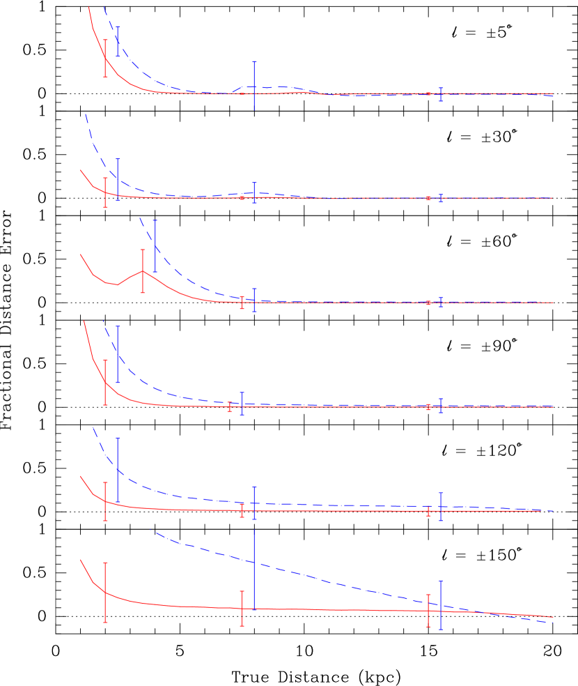
Figure 3: Fractional distance error versus true distance for simulated data with 7 km s^-1 (red lines) and 20 km s^-1 (blue dashed lines) random noise added. Lines are unweighted averages of 10,000 random trials sampled every 0.5 kpc; representative single-trial error bars indicate standard deviations about the mean. Galactic longitudes are indicated in the top right of each panel, with the $\pm$ symbol indicating that the same plot holds for both longitudes. Note the significant bias of 3D kinematic distance estimates, which grow toward the origin as the inverse of true distance. See Section 4 for more discussion.

5 Effects of Systematic Errors

The 3D kinematic distance method requires accurate values for the Galaxy’s fundamental parameters: the distance to the Galactic center (${R_{0}}$), the circular rotation speed at the Sun (${\Theta_{0}}$), and its rotation curve. Fortunately, the BeSSeL Survey and the VERA project have provided hundreds of parallaxes and proper motions for massive and extremely young ($<1$ My) stars, and these have been modeled to give accurate estimates of ${R_{0}}=8.15\pm 0.15$ kpc and ${\Theta_{0}}=236\pm 7$ km s^-1 (Reid et al., 2019). These values are independently confirmed by 1) infrared observations tracing stars orbiting the supermassive black hole, Sgr A*, at the center of the Galaxy, giving ${R_{0}}=7.946\pm 0.059$ kpc (Do et al., 2019) and ${R_{0}}=8.275\pm 0.034$ kpc (Gravity Collaboration et al., 2021), for which a variance-weighted average is ${R_{0}}=8.19$ kpc, and 2) the apparent proper motion in longitude of Sgr A* (giving the reflex of the Sun’s orbital motion in the Galaxy) of $6.411\pm 0.008$ mas y^-1 (Reid & Brunthaler, 2020), which translates to ${\Theta_{0}}=236\pm 2$ km s^-1, after subtracting the Sun’s peculiar motion of $12\pm 2$ km s^-1 (Schönrich, Binney & Dehnen, 2010) in the direction of Galactic rotation.

The BeSSeL Survey and VERA project measurements also, provide a “gold standard” rotation curve, based on parallax distances and 3D velocities, between Galactocentric radii (R) of 4 to 15 kpc (Reid et al., 2019). Thus, inaccuracies in the model of the Galaxy are not likely to have a significant effect on 3D kinematic distances over this range of radii. However, inside of 5 kpc the observational constraints for the adopted “universal” rotation curve model become weaker. In order to assess the accuracies of 3D kinematic distances in the central 5 kpc, we simulate uncertainty in the model rotation curve by adding rms deviations which grow linearly from 0 km s^-1 at $R=5$ kpc to 50 km s^-1 at $R=0$ kpc. When adding random speeds to the rotation curve values in simulated trials, we do not allow rotation speed to drop below 50 km s^-1.

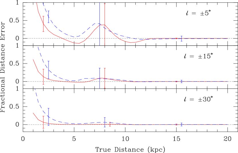
Figure 4: Fractional distance error versus true distance for simulated data allowing for significant uncertainty in the assumed rotation curve speed within 5 kpc of the Galactic center (at a distance of 8.15 kpc from the Sun) in addition to random motions. See Fig. 3 caption for other details.

Fig. 4 shows the effects of errors in the assumed rotation curve for three Galactic longitudes for which the minimum Galactic radii are less than 5 kpc. At longitude $30{{}^{\circ}}$ there is no noticeable change in fractional distance uncertainty compared to that shown in Fig. 3, since the minimum radius (at the tangent point distance of 8.1 kpc) is 4.1 kpc, and so at no distances do we add more than 9 km s^-1 noise to the trial rotation curves. Noticeable effects are evident for the longitude $15{{}^{\circ}}$ plot, where the minimum Galactic radius is 2.1 kpc and up to 29 km s^-1 rms noise is added to the rotation curve. However, at $5{{}^{\circ}}$ longitude, where the minimum radius is only 0.7 kpc and up to 43 km s^-1 noise is added, there are significant fractional distance errors over a range of distances from about 5 to 11 kpc.

Fig. 5 shows the effects of anomalous motions seen in massive young stars near the end of the Galactic bar (Immer et al 2019). These anomalous motions peak at $\approx 40$ km s^-1 and are mostly directed toward the Galactic center. For the near end of the bar in Galactic quadrant 1, we model these anomalies with a Gaussian distribution, centered at longitude $27{{}^{\circ}}$ and a Galactocentric radius of 4.5 kpc, and decreasing with offset with a $1\sigma$ scale-length of 2 kpc. The bottom panel of Fig. 5 indicates that for sources at Galactic longitude $+30{{}^{\circ}}$ and distances from the Sun of 4 to 7 kpc, one sees an $\approx 10$% bias toward smaller values of 3D kinematic distances. For the far end of the bar in Galactic quadrant 4, we also model these anomalies with a Gaussian distribution, but centered at longitude $-13{{}^{\circ}}$ and a Galactocentric radius of 12 kpc. The top panel of Fig. 5 indicates that for sources at Galactic longitude $-15{{}^{\circ}}$ and at distances from the Sun of 11 to 13 kpc, one again sees an $\approx 10$% bias toward smaller values of 3D kinematic distances. These bias are similar for the cases of 7 km s^-1 (solid red lines) and 20 km s^-1 (dashed blue lines) added noise, since the anomalous motions are systematic and tend to dominate.

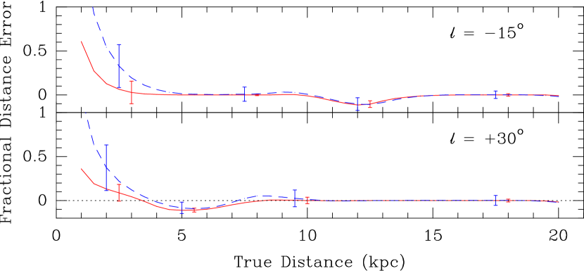
Figure 5: Fractional distance error versus true distance for simulated data allowing for anomalous motions near the end of the Galactic bar toward the Galactic center in addition to random motions. The far end of the bar is near $-15{{}^{\circ}}$ at 12 kpc (top panel). The near end of the bar is near $+30{{}^{\circ}}$ at 4 kpc (bottom panel). See Fig. 3 caption for other details.

6 Conclusions and Outlook

In this paper, we have examined the precision and accuracy of 3D kinematic distance estimates in several ways. First, we compared these estimates against trigonometric parallax distances for large numbers of masers associated with massive young stars. These demonstrated a good corresponce between the two methods for stars with distances $\mathrel{\hbox{\raise 2.15277pt\hbox{$>$}\hbox to0.0pt{\hss\lower 2.15277pt\hbox{$\sim$}}}}8$ kpc, and indicated that 3D kinematic distances can be more accurate than parallax measurments. For more nearby stars, 3D kinematic distances displayed a modest bias of $\approx 1$ kpc toward larger distances.

In order to better assess accuracies and biases for 3D kinematic distances, we simulated large numbers of sources with (1D) random motions of 7 and 20 km s^-1 and evaluated the statistical properties of such distances estimates. Random motions of 7 km s^-1 per velocity component (corresponding to 12 km s^-1 for the full velocity magnitude) are representative of Viral motions of within giant molecular clouds. For these simulations, we find excellent performance of 3D kinematic distances (ie, negligible bias and fractional distance uncertainty less than 10%) for true distances $\mathrel{\hbox{\raise 2.15277pt\hbox{$>$}\hbox to0.0pt{\hss\lower 2.15277pt\hbox{$\sim$}}}}5$ kpc. For smaller distances, a positive bias of $\approx 20$% of the true distance is generally seen at 2 kpc true distance and scales with the inverse of true distance. Additional positive biases are seen near tangent point distances of 4 to 8 kpc for Galactic longitudes of $60{{}^{\circ}}$ and $5{{}^{\circ}}$, where line-of-sight velocity gradients are small and secondary peaks in the distance PDFs can become favored.

We also used simulations to assess the effects of systematic errors in the assumed rotation curve in the inner Galaxy, as well as for a region near the end of the Galactic bar where large non-circular motions have been noted. For distances near 8 kpc and Galactic longitudes $\mathrel{\hbox{\raise 2.15277pt\hbox{$<$}\hbox to0.0pt{\hss\lower 2.15277pt\hbox{$\sim$}}}}15{{}^{\circ}}$, uncertainty in the rotation curve produces a noticeable increase in dispersion in distance estimates, and at longitude $5{{}^{\circ}}$ the dispersion becomes comparable to distance. Anamalous motions, as seen for massive young stars near the end of the Galactic bar in Galactic quadrant 1, generally produce negative 3D kinematic distance biases of $\mathrel{\hbox{\raise 2.15277pt\hbox{$<$}\hbox to0.0pt{\hss\lower 2.15277pt\hbox{$\sim$}}}}10$%.

Simulations assuming large random 1D velocities of 20 km s^-1 (corresponding to 3D magnitudes of 35 km s^-1), as would be expected produce larger dispersions and biases compared to the 7 km s^-1 simulations. However, for Galactic longitudes with magnitudes $\mathrel{\hbox{\raise 2.15277pt\hbox{$<$}\hbox to0.0pt{\hss\lower 2.15277pt\hbox{$\sim$}}}}120{{}^{\circ}}$ and distances $\mathrel{\hbox{\raise 2.15277pt\hbox{$>$}\hbox to0.0pt{\hss\lower 2.15277pt\hbox{$\sim$}}}}10$ kpc, 3D kinematic distances still perform very well.

3D kinematic distances have some obvious applications. Directly mapping the spiral structure of the Milky Way has proven to be a challenging enterprise, since distances are very large and dust extinction blocks most of the Galactic plane at optical wavelengths. Thus, Gaia, even with a parallax accuracy approaching $\pm 0.01$ mas, cannot freely map the Galactic plane. However, VLBI is unaffected by extinction and can detect masers associated with young stars that best trace spiral structure. While a parallax with 12% accuracy has been measured for a water maser associated with a massive young star on the far side of the Milky Way at 20 kpc distance, obtaining large numbers of such measurements would require an enormous amount of observing time. However, for such distant massive, young stars (with random 1D motions near 7 km s^-1), 3D kinematic distances have intrinsic accuracy better than can generally be achieved with parallax measurements, and they can be obtained for large numbers of stars with only modest amounts of observing time. This will facilitate tracing spiral structure across the entire Milky Way.

Finally, we note that knowledge of distance to X-ray binaries is crucial to understanding their nature. For example, a trigonometric parallax-distance measurement of 2.22 kpc for Cyg X-1 firmly established that this binary system contains a black hole and a massive young star (Miller-Jones et al., 2021). However, accurate trigonometric parallax measurements for more distant binaries have proven difficult to obtain, e.g.,  GRS 1915 (Reid et al., 2014). Since proper motions can be measured far more easily than parallaxes, for distant binaries with modest peculiar motions, 3D kinematic distances can provide reliable distances.

References

- Do et al. (2019) Do, T., Hess, A., Ghez, A. et al. (2019), Sci, 365, 664
- Gravity Collaboration et al. (2021) Gravity Collaboration, Abuter, R. Amorim, A. et al. 2021, A&A, 647, 59
- Immer et al. (2019) Immer, K., Li, J., Quiroga-Nunez, L. H. et al. 2019, A&A, 632, 123
- Miller-Jones et al. (2021) Miller-Jones, J. A., Bahramian, A., Orosz, J. A. et al. 2021, Sci, 371, 1046
- Persic, Salucci & Stel (1996) Persic, M., Salucci, P. & Stel, F. 1996, MNRAS, 281, 27
- Reid et al. (2009) Reid, M. J., Menten, K. M., Zheng, X. W. et al. 2009, ApJ, 700, 137
- Reid et al. (2014) Reid, M. J., McClintock, J. E., Steiner, J. F. et al. , 2014, ApJ, 796, 2
- Reid et al. (2019) Reid, M. J., Menten, K. M., Brunthaler, A. et al. 2019, ApJ, 885, 131
- Reid & Brunthaler (2020) Reid, M. J. & Brunthaler, A. 2020, ApJ, 892, 39
- Sanna et al. (2017) Sanna, A., Reid, M. J., Dame, T. M., Menten, K. M. & Brunthaler, A. 2017, Sci, 358, 227
- Schönrich, Binney & Dehnen (2010) Schönrich, R., Binney, J. & Dehnen, W. 2010, MNRAS, 403, 1829
- Sofue (2011) Sofue, Y. 2011, PASJ, 63, 813
- Yamauchi et al. (2016) Yamauchi, A., Yamashita, K., Honma, M., Sunada, K. & Nakagawa, A. et al. 2016, PASJ, 68, 60