Symmetry Breaking in Bose-Einstein Condensates Confined by a Funnel Potential

Abstract

In this work, we consider a Bose-Einstein condensate in the self-focusing regime, confined transversely by a funnel-like potential and axially by a double-well potential formed by the combination of two inverted Pöschl-Teller potentials. The system is well described by a one-dimensional nonpolynomial Schrödinger equation, for which we analyze the symmetry break of the wave function that describes the particle distribution of the condensate. The symmetry break was observed for several interaction strength values as a function of the minimum potential well. A quantum phase diagram was obtained, in which it is possible to recognize the three phases of the system, namely, symmetric phase (Josephson), asymmetric phase (spontaneous symmetry breaking - SSB), and collapsed states, i.e., those states for which the solution becomes singular, representing unstable solutions for the system. We analyzed our symmetric and asymmetric solutions using a real-time evolution method, in which it was possible to confirm the stability of the results. Finally, a comparison with the cubic nonlinear Schrödinger equation and the full Gross-Pitaevskii equation were performed to check the accuracy of the effective equation used here.

I Introduction

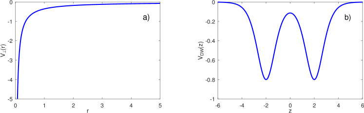
Figure 1: The trapping potential in the (a) transverse and (b) axial direction, given by Eqs. (1) and (4), respectively, by considering $V_{0}=0.8$, $z_{0}=\pm 2,~{}a=1$ and $\varepsilon=1$.

The interactions of light and matter consists of one of the most fundamental aspects used for the realization of Bose-Einstein condensates (BECs). Indeed, since the first realizations in diluted atomic gases of alkali metals at ultra-low temperatures Anderson et al. (1995); Davis et al. (1995); Bradley et al. (1995), several phenomena have been observed, such as formation of matter-wave dark Burger et al. (1999) and bright Kh. Abdullaev et al. (2005); Cornish et al. (2006); Khaykovich et al. (2002) solitons, generation of vortex states Matthews et al. (1999); Madison et al. (2000), the engineering of spin–orbit-coupled BECs Lin et al. (2011), Anderson localization of matter waves Billy et al. (2008); Roati et al. (2008), quantum droplets Cabrera et al. (2018); Cheiney et al. (2018); Semeghini et al. (2018); D’Errico et al. (2019), etc.

In this context, BECs trapped by double-wells potentials have been studied in recent decades, presenting advances from a theoretical point of view Yuan and Ding (2005); Xie et al. (2015); Shchesnovich et al. (2004); Salasnich and Malomed (2011); Mazzarella et al. (2009); Mazzarella and Salasnich (2010). In Ref. Shchesnovich et al. (2004), families of bright solitons were investigated in binary BECs, trapped by asymmetric double-well potentials. In particular, when the scattering lengths of each component of the BEC have opposite signs, the results (numerical and analytical) showed stability with weak repulsive interaction. BECs trapped in double square well and optical lattice well were also investigated in Ref. Yuan and Ding (2005).

An important phenomenon present in some systems trapped by double-well potentials (or similar) is the spontaneous symmetry breaking (SSB), which is a characteristic of the ground state presenting an asymmetry with respect to the axis defined by the potential. In this sense, in Ref. Salasnich and Malomed (2011) a coupled disk-shaped BECs, showed symmetry breaking in a self-attractive and coupling weak regime. Even in an almost 2D regime, bifurcation diagrams show a direct relationship between symmetry, asymmetry and the norm of the solitons of a system trapped in a double-channel potential (BECs or optical systems) (see Ref. Matuszewski et al. (2007) for more details). In the one-dimensional case, single Mazzarella and Salasnich (2010) and binary Mazzarella et al. (2009) BECs were reported to present symmetry breaking. Furthermore, the symmetry breaking in BECs can be induced by the nonlinearity coefficient Mayteevarunyoo et al. (2008). In this case, the spatial dependent nonlinearity obtained by means of the spatially inhomogeneous Feshbach resonance, acts as a pseudo double-well potential.

In all the above-mentioned works there is the presence of some method of dimensional reduction to describe the system by an effective 1D or 2D equation. However, the models under consideration (BECs and some types of optical systems) are generally described by a three-dimensional (3D) nonlinear Schrödinger equation (NLSE), that require a lot of computational effort to be solved numerically. On the other hand, in Ref. Salasnich et al. (2002) the authors presented a dimensional reduction method via a variational approach in order to obtain an effective equation that correctly describes the longitudinal (transversal) profile of the BEC. This technique has been extensively tested for decades, showing great results Salasnich and Malomed (2009); Salasnich (2009); Young-S. et al. (2010); Cardoso et al. (2011); Salasnich and Malomed (2012); dos Santos and Cardoso (2019); dos Santos et al. (2020, 2019, 2021). In the case of BECs, starting from the Gross-Pitaevskii (GP) equation (a NLSE type), this approach allows us to derive a nonpolynomial Schrödinger equation (NPSEs), which describes the reduced dynamics of the corresponding physical system. Several configurations have been investigated and recently in Refs. dos Santos et al. (2019, 2021) the authors studied a BEC confined by a radial singular potential ($\sim 1/r$), demonstrating the effectiveness of NPSE in describing the longitudinal behavior of the ultracold gas even when confined by anharmonic potentials. This configuration, called the funnel shape, can be achieved using a vapor of magnetic atoms attracted by an axial electric current.

In this paper we investigated the funnel-shaped BEC loaded into the symmetric double-well potential (axial direction). This system is well described by a NPSE dos Santos et al. (2019, 2021), for which we obtain three types of ground-states: symmetric, asymmetric and collapsed states. Symmetric solutions present densities with even parity, i.e., the particle density is invariant by changing the sign of its spatial coordinate. Asymmetric profiles exhibit the opposite behavior to that shown by the symmetric case, i.e., they do not show sign inversion symmetry of the spatial coordinate. Finally, the system can also present the collapsed states, which have energy equal to minus infinity Sakellari et al. (2004). We present the quantum phase diagram of the funnel-shaped BEC and study how the characteristics of this confinement affect the phase of the condensate. The quantum phase of a NPSE obtained from a BEC transversely confined by a harmonic oscillator was studied in Ref. Mazzarella and Salasnich (2010). Differently, here we will show results from a singular, but physical potential, presenting a correlation between the phase and the transversal confinement. Finally, we studied the stability of the symmetrical and asymmetrical profiles, in addition to presenting coherent oscillations of matter (population imbalance) produced by abrupt changes in the double-well potential.

II Theoretical model

Let us consider a system formed by a dilute quantum gas, with attractive interaction properties, at absolute zero temperature Pethick and Smith (2008). The system is trapped by a superposition of a funnel shape potential in the transverse direction dos Santos et al. (2019) and a double-well potential in the axial direction ($z$). This double-well is formed by the combination of two inverted Pöschl-Teller potentials, represented by $V_{\textrm{DW}}(z)$:

$$V_{\mathrm{DW}}(z) = V_{L}(z)+V_{R}(z),$$ (1)

$$V_{L}(z) = -V_{0}\left[\textrm{sech}^{2}\left(\frac{z+z_{0}}{a}\right)\right],$$ (2)

$$V_{R}(z) = -V_{0}\left[\textrm{sech}^{2}\left(\frac{z-z_{0}}{a}\right)\right].$$ (3)

The funnel-shaped potential, acting in the transverse $(x,y)$ plane, is given by

$$V_{\perp}(r)=-\frac{\varepsilon^{3}}{2r},$$ (4)

where $\varepsilon>0$ is a constant with dimension of length and the radial coordinate is defined as $r\equiv\sqrt{x^{2}+y^{2}}$. As an example, we display the potentials in Fig. 1.

Thus, the complete trapping potential can be written as

$$V_{\textrm{trap}}(r,z)=-\frac{\varepsilon^{3}}{2r}+V_{\mathrm{DW}}(z).$$ (5)

The macroscopic wave function that describes the behavior of this system is governed by the GP equation Dalfovo et al. (1999)

$$i\hbar\frac{\partial}{\partial t}{\psi}(\textbf{r},t)=\left[-\frac{\hbar^{2}}{2m}\nabla^{2}+V(r,z)+Ng\left|\psi(\textbf{r},t)\right|^{2}\right]\psi(\textbf{r},t).$$ (6)

where $g=4\pi\hbar^{2}a_{s}/m$ is the coupling constant directly proportional to the scattering length $a_{s}$, $N$ is the number of particles, $m$ is the atomic mass, and $\nabla^{2}$ is the standard Laplacian operator in three dimensions. By means of a rescale of the variables $t\rightarrow\omega_{\perp}t$, $(x,y,z)\rightarrow(x,y,z)/a_{\perp}$, $\psi\rightarrow\psi a_{\perp}^{3/2}$ and $V\rightarrow V/\hbar\omega$, with $a_{\perp}=\sqrt{\hbar/m\omega_{\perp}}$, in Eq. (6), one obtains

$$i\frac{\partial\psi}{\partial t}=-\frac{1}{2}\nabla^{2}\psi+V(r,z)\psi+2\pi\Gamma|\psi|^{2}\psi.$$ (7)

with $\Gamma=2a_{s}N/a_{\perp}$. The Lagrangian density that corresponds to Eq. (7), with the potential (5), is given by

$$\mathcal{L} = \frac{i}{2}\left(\psi^{*}\frac{\partial\psi}{\partial t}-\psi\frac{\partial\psi^{*}}{\partial t}\right)-\frac{1}{2}|\nabla\psi|^{2}$$ (8)

$$- \left(V_{\textrm{DW}}(z)-\frac{\varepsilon^{3}}{2r}\right)|\psi|^{2}-\pi\Gamma|\psi|^{4}.$$

Our goal is to reduce the 3D model to an effective 1D equation. In a didactic way, we recall here the deduction of the effective equation shown in Ref. dos Santos et al. (2019), where we use the following ansatz

$$\psi(r,z,t)=\exp\left(-\frac{r}{2\eta^{2}}\right)\frac{f(z,t)}{\sqrt{2\pi}\eta^{2}},$$ (9)

where $f(z,t)$ is an axial complex wave function and $\eta=\eta(z,t)$ is the transverse length with the normalization condition

$$\int_{-\infty}^{+\infty}|f(z)|^{2}dz=1,$$ (10)

required to ensure the unitary normalization of the wave function in 3D. Inserting the ansatz into the Lagrangian density (Eq. (8)) we must to perform the integration on the transversal plane $(x,y)$ and neglect the derivatives that include terms like $\partial\eta/\partial z$ Salasnich et al. (2002). Then, we obtain the effective Lagrangian in one dimension written as

$$L_{1D} = \int_{-\infty}^{\infty}\Bigg{[}\frac{i}{2}\left(f^{*}\frac{\partial f}{\partial t}-f\frac{\partial f^{*}}{\partial t}\right)-\frac{1}{2}\left|\frac{\partial f}{\partial z}\right|^{2}-\frac{\Gamma}{8}\frac{|f|^{4}}{\eta^{4}}$$ (11)

$$- \left[V_{\textrm{DW}}+\frac{1}{2\eta^{2}}\left(\frac{1}{4\eta^{2}}-\varepsilon^{3}\right)\right]|f|^{2}\Bigg{]}dz.$$

The following step is to use the Euler-Lagrange equation

$$\frac{\partial\mathcal{L}}{\partial\varphi}-\frac{\partial}{\partial t}\frac{\partial\mathcal{L}}{\partial\dot{\varphi}}-\frac{\partial}{\partial z}\frac{\partial\mathcal{L}}{\partial\varphi_{z}}=0,$$ (12)

for both $f$ and $\eta$ terms ($\varphi\equiv f,\eta$). The results consist of two coupled equations:

$$i\frac{\partial f}{\partial t}=-\frac{1}{2}\frac{\partial^{2}f}{\partial z^{2}}+V_{\textrm{DW}}(z)f+\frac{1}{2\eta^{2}}\left(\frac{1}{4\eta^{2}}-\varepsilon^{3}\right)f+\frac{\Gamma|f|^{2}}{4\eta^{4}}f,$$ (13)

$$2\varepsilon^{3}\eta^{2}-1-\Gamma|f|^{2}=0.$$ (14)

Inserting Eq. (14) into Eq. (13) we obtain the time-dependent 1D NPSE

$$i\frac{\partial f}{\partial t}=-\frac{1}{2}\frac{\partial^{2}f}{\partial z^{2}}+V_{\textrm{DW}}(z)f-\frac{\varepsilon^{6}}{2(1+\Gamma|f|^{2})^{2}}f,$$ (15)

which will be the main model used in our simulations. Indeed, the effective equation Eq. (15) describes the dynamics of a BEC confined in the transverse plane by a funnel-shaped potential and axially by a double-well (Eq. (5)). Additionally, the nonlinear regimes of strong and weak interaction can be obtained in a simplified way through approximations. A BEC in the weak interaction regime implies that the relation $\Gamma|f|^{2}\ll 1$ is valid Pethick and Smith (2008). Using this approximation in the above NPSE and expanding the nonpolynomial term in terms of $\Gamma|f|^{2}$, we get the nonlinear cubic Schrödinger equation, given by

$$i\frac{\partial f}{\partial t}=-\frac{1}{2}\frac{\partial^{2}f}{\partial z^{2}}+V(z)f-\varepsilon^{6}\left(\frac{1}{2}-\Gamma|f|^{2}\right)f.$$ (16)

Next, by considering a system with repulsive interatomic interaction and in a strong interaction regime, we can make use of the well-known Thomas-Fermi (TF) approximation Pethick and Smith (2008), which neglects the contribution of spatial derivatives, i.e., the contribution of kinetic energy is much smaller when compared to the interaction between the particles. In order to obtain a one-dimensional equation for this regime, we must substitute into the Eq. (6) a normalized wave function, given by dos Santos et al. (2019)

$$\psi(\textbf{r},t)=e^{-i\mu t}\frac{f(z)}{\sqrt{(2\pi)}}e^{-r/2},$$ (17)

which corresponds to the initial ansatz, Eq. (9), with $\eta=1$. Carrying out the integrations on $x$ and $y$, we get the following result for the density distribution in $z$-direction

$$|f(z)|^{2} = \begin{cases}\dfrac{9}{4\Gamma}\left[4\mu-4V(z)+\varepsilon^{3}\right],&\;\text{for}\ \mu+\varepsilon^{3}/4>V(z)\\ 0,&\;\text{for}\ \mu+\varepsilon^{3}/4\leq V(z),\end{cases}$$

which corresponds to the TF solution. In the next section we discuss the physical effects of the inclusion of the double-well potential in $z-$coordinate on the emergence of broken symmetry states.

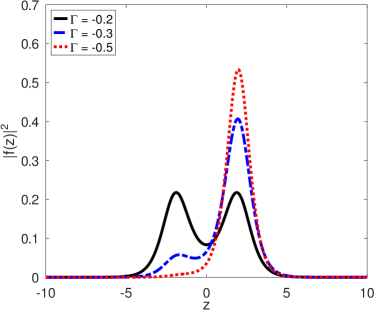
Figure 2: Axial probability density, $|f(z)|^{2}$, of the ground state for different values of the interaction strength ($\Gamma$), considering an attractive BEC trapped by a funnel potential in the transverse direction and a double-well potential in the axial direction.

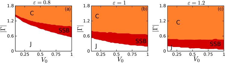
Figure 3: Quantum phase diagram of interaction strength $\Gamma$ vs the double-well depth $V_{0}$ for the NPSE. Three different values of the strength of the funnel-shaped potential are used here, i.e., (a) $\varepsilon=0.8$, (b) $\varepsilon=1.0$, and (c) $\varepsilon=1.2$. The different regions are represented by Josephson phase (J), spontaneous symmetry breaking (SSB), and collapsed states (C), the latter representing the regions whose numerical results present singularities.

III Results

First, we present the results of the imaginary-time evolution of the 1D NPSE (15). Indeed, by means of imaginary-time evolution one can obtain the ground states of the system under consideration. To this end, we have employed a second-order split step method to solve this equation numerically. As an example, in Fig. 2 we plot the axial probability density of the wave function for three different values of the interaction strength ($\Gamma$) in order to elucidate the presence of SSB in the system. Note that for $\Gamma=-0,2$ the solution is symmetrical with respect to the double-well center, characterizing a state known as the Josephson phase (J). For $\Gamma<-0.2$ the metastable state solution becomes asymmetric and the phenomenon of SSB occurs. Finally, for $\Gamma=-0.5$, the BEC is essentially localized in the right well. For values of $\Gamma<-0.7$ the equation does not predict a possible solution, i.e., we get a singularity from the numerical results and the configuration of the condensate collapses in a nonphysical state.

Further, we analyzed the behavior of the solution of the effective NPSE (15) for different values of $V_{0}$ and the modulus of $\Gamma$, in order to establish a phase diagram for the BEC states. The results are displayed in Fig. 3. Note that the region presenting symmetrical phase (J) shrinks as we increase the $\varepsilon$ value, while the region with collapsed states (C) increases. However, the region presenting asymmetric solutions (SSB) does not significantly change its shape but presents a shift to smaller $\Gamma$ values as $\varepsilon$ increases. This result emphasizes the importance of controlling the transverse confinement on the solutions to be obtained.

Next, in order to compare our results with those from the other equations, we investigated the solutions of GP equation and cubic NLSE, represented respectively by Eqs. (6) and (16), carrying out the calculations for various values of $\Gamma$, keeping the value $V_{0}=0.8\hbar\omega_{\perp}$. The results are summarized in Fig. 4. The most relevant result is the confirmation of the symmetry breaking by the GP equation in a perfect accuracy with the results obtained from the effective NPSE. It is observed that the cubic NLSE reveals an inaccuracy regarding to the GP equation for all asymmetric cases. For example, in Fig. 4(b) with $\Gamma=-0.25$ the cubic equation indicates an axial probability density, $|f(z)|^{2}$, symmetric about the origin while the GP equation clearly refers to a symmetry breaking, likewise to the effective equation, demonstrating better accuracy than the previous one.

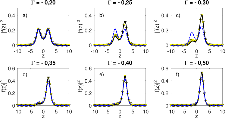
Figure 4: Density profile obtained from the NPSE (black solid line), cubic NLSE (blue dashed line), and GP equation (yellow triangles) by considering different values of interaction strengths ($\Gamma$).

The above results ensure the accuracy of the effective equation against the results obtained for the ground states of the GP equation. Following, we carried out calculations to attest the stability of our results and to analyze the dynamics of the density profile of the BEC. To this end, we use a real-time evolution method that uses as input solution the ground-state obtained via imaginary-time propagation method plus a $10\%$ of white noise in its amplitude profile. Next, we consider two different situations in our analyses, namely, unaltered double-well potential (i.e., as described by Eq. (1)) and a double-well with sudden displacement in its depth ($V_{0}$).

The results of the case dealing with the unaltered potential are shown in Fig. 5. In the upper panels we exhibit the input profiles, with (a) being a symmetric input state while in (b), (c) and (d) we have asymmetric input states. It is observed in the central panels the stability of the propagation of the solutions up to $t=2000$ and in the lower panels the corresponding small oscillations of expected value of z (i.e., $\langle z\rangle$). As a consequence of these results, one can observe that all states are dynamically stable in the face of perturbations added to the ground states analyzed here.

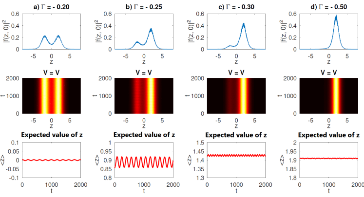
Figure 5: Real time simulations of perturbed ground states of NPSE for different values of $\Gamma$ (represented by the upper panels (a)-(d)). In the middle panels the 3D profiles of the evolution of the input solutions are shown, while in the respective lower panels we present the behavior of the temporal evolution of the mean value of z ($\langle z\rangle$).

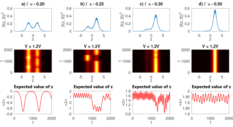
Figure 6: Real time simulations of perturbed ground states of NPSE with a boosted amplitude double-well potential for different values of $\Gamma$ (represented by the upper panels (a)-(d)). In the middle panels the 3D profiles of the evolution of the input solutions are shown, while in the respective lower panels we present the behavior of the temporal evolution of the mean value of $z$ ($\langle z\rangle$).

In the second case of analyzing the dynamics of the solutions, we include an instantaneous increase in the depth of the potential, given by:

$$V\rightarrow 1.2\times\left(V_{\mathrm{DW}}\right).$$ (19)

This sudden adjustment caused more noticeable periodic oscillations in our system, as can be seen in the results displayed in Fig. 6. We used the same $\Gamma$ values for the input solutions and analyzed the evolution in real time evolution under the same parameters as in the previous case. Despite the oscillations in the expected value of z (lower panels), it appears that the solutions are robust by observing the evolutions obtained in the central panels. By observing the column (a) of Fig. 6, which represents the evolution of the symmetric state, it is interesting to note that the figure in the central panel has its maximum oscillating for negative values of $z$, that is, going to the left well and restoring the initial position after some time, displaying a pattern like Josephson oscillations Mazzarella et al. (2009); Mazzarella and Salasnich (2010). In fact, the well in which the system is headed is arbitrary and here we represent only the cases in which the solution led to the right. In column (b) we have an asymmetric input solution, with a higher probability density on the right well, and after some time the oscillations of the particles between the two wells can be seen, highlighted by the variation of the potential module, when compared to the same evolution with the fixed potential. This behavior is emphasized by the expected value of $z$, shown in the lower panel. Finally, in columns (c) and (d) we present the evolution of the profiles obtained with $\Gamma=-0.30$ and $-0.50$, respectively. It is important to note that decreasing self-interaction $\Gamma$ decreases the amplitude of $\langle z\rangle$ oscillations. For example, in (c) the maximum percentage variation of the expected value $|\langle z\rangle_{maximum}-\langle z\rangle_{minimum}|/\langle z\rangle_{maximum}$ is 54%, while (d) presents approximately 5%.

IV Conclusion

In conclusion, we investigated the influence of a transversal funnel-like potential on the SSB inherent to the longitudinal profile of a BEC. We derived an effective NPSE that accurately describes the longitudinal profile of the system, for which we analyze the SSB of the wave function. The symmetry break was observed for several interaction strength values as a function of the minimum potential well. Our results confirmed that this system experiences a symmetry break in perfect agreement with the results obtained from the 3D GP equation. We observed a quantum phase diagram presenting three distinct types of solutions, i.e., symmetric phase (Josephson phase), the SSB phase and the values representing the collapsed state (unstable states). Furthermore, we analyzed the obtained symmetric and asymmetric solutions by using a real-time evolution method, in which it was possible to confirm the stability of the results.

These results show that the form of confinement of the BEC can change static and dynamic patterns associated with SSB of the system. In addition, the effective NPSE derived in Ref. dos Santos et al. (2019) can be used to correctly describe the system even in the presence of SSB.