LASSO reloaded: a variational analysis perspective with applications to compressed sensing

Abstract

This paper provides a variational analysis of the unconstrained formulation of the LASSO problem, ubiquitous in statistical learning, signal processing, and inverse problems. In particular, we establish smoothness results for the optimal value as well as Lipschitz and smoothness properties of the optimal solution as functions of the right-hand side (or measurement vector) and the regularization parameter. Moreover, we show how to apply the proposed variational analysis to study the sensitivity of the optimal solution to the tuning parameter in the context of compressed sensing with subgaussian measurements. Our theoretical findings are validated by numerical experiments.

49J53, 62J07, 90C25, 94A12, 94A20

1 Introduction

One of the most important problems in the applied mathematical sciences is to recover a signal $x_{0}\in\mathbb{R}^{n}$ from noisy linear measurements $b=Ax_{0}+h\in\mathbb{R}^{m}$, where $A\in\mathbb{R}^{m\times n}$ is a measurement (or sensing) matrix and $h\in\mathbb{R}^{m}$ is a noise vector. A fundamental observation is that such a linear inverse problem can be assumed (or cast to) have sparse solutions, which can be recovered with high probability from $m\ll n$ (random) observations via computationally efficient signal reconstruction strategies. This is well documented in the groundbreaking work by Donoho [18] and Candès, Romberg, and Tao [15, 16], which gave rise to the field of compressed sensing. Since its introduction, the compressed sensing paradigm led to major technological advances in a vast array of signal processing applications, such as, most notably, compressive imaging. For an introduction to the field, its applications, and historical remarks, we refer the reader to [2, 20, 22, 33, 56].

In the noiseless setting (i.e., when $h=0$), the sparse recovery paradigm for linear inverse problems manifests itself in the optimization framework

(1) $$\min_{x\in\mathbb{R}^{n}}\|x\|_{0}\ \mbox{s.t.}\ Ax=b,$$

where $\|\cdot\|_{0}$ is counting the nonzero entries of a vector in $\mathbb{R}^{n}$. Despite the absence of noise, problem Eq. 1 is provably NP-hard in general [22, 39]. Thus, many convex relaxations of this optimization problem have been proposed, all of which, in essence, rely on the fact that the $\ell_{1}$-norm is the convex envelope of $\|\cdot\|_{0}$ restricted to an $\ell_{\infty}$-ball (see, e.g., [2, §D.4]).

Here we focus on sparse recovery via $\ell_{1}$ minimization in the noisy setting (i.e., when $h\neq 0$) based on the well-known (unconstrained) LASSO (Least Absolute Shrinkage and Selection Operator) problem

(2) $$\min_{x\in\mathbb{R}^{n}}\frac{1}{2}\|Ax-b\|^{2}+\lambda\|x\|_{1},$$

where $\lambda>0$ is a regularization (or tuning) parameter and where $\|\cdot\|$ and $\|\cdot\|_{1}$ denote the $\ell_{2}$- and $\ell_{1}$-norm, respectively. To the best of our knowledge, the LASSO problem was originally proposed by Santosa and Symes [46] and then introduced (in a constrained formulation) by Tibshirani in the context of statistical regression [51]. Since then, the LASSO has become an indispensable tool in statistical learning, especially when performing tasks such as model selection (see [26] and references therein). Moreover, it plays a key role in Bayesian statistics, thanks to its ability to characterize maximum a posteriori estimators in linear regression when the parameters have independent Laplace priors [42]. We also note that problem Eq. 2 was introduced in signal processing by Chen, Donoho, and Saunders in [17] under the name of basis pursuit denoising. Here on, we refer to the unconstrained LASSO simply as the LASSO.

From the optimization perspective, the LASSO falls into the category of (additive) composite problems, for which many numerical solution methods have been devised and which have been tested on Eq. 2, including proximal gradient methods (e.g., FISTA [11]) and primal-dual methods, see Beck’s excellent textbook [6] for references, or proximal Newton-type methods proposed by Lee et al. [34], Khanh et al. [32], Kanzow and Lechner [31] or Milzarek and Ulbrich [36].

From the perspective of variational analysis [13, 19, 37, 38, 45], given any optimization problem with parameters, the question as to the behavior of the optimal value and the optimal solution(s) as functions of the parameters arises naturally. The trifecta for solutions of any optimization problem is: existence, uniqueness and stability. For the LASSO problem, existence is easily established as the $\ell_{1}$-norm is coercive (and the quadratic term is not counter-coercive). Sufficient conditions for uniqueness were established by Tibshirani [52] and Fuchs [25, Theorem 1]. A set of conditions (see Section 4.1 below) that characterizes uniqueness of solutions of a whole class of $\ell_{1}$-optimization problems (including the LASSO) were established by Zhang et al. [58]. An alternative, shorter proof (even though it is not explicitly stated for the LASSO) of this characterization was given by Gilbert [27] which relies, in essence, on polyhedral convexity. Stability results for the LASSO are somewhat scattered throughout the literature. Previous work has examined sensitivity of various formulations of $\ell_{1}$ optimization techniques with respect to the choice of the tuning parameter; and other work has examined their robustness to, e.g., measurement error [1, 23]. Regarding the selection of the tuning parameter, the choice of the optimal parameter has been well-studied. In the case of LASSO, the optimal choice of tuning parameter was analyzed in [12] and [47] in such a way as to yield a notion of stability for all sufficiently large $\lambda$. Other work has characterized the recovery error for LASSO in terms of the tuning parameter, but does not discuss notions of sensitivity [5, 41, 49, 50]. An asymptotic result establishing sensitivity of the error when $\lambda$ is less than the optimal choice has been exhibited in a closely related simplification [9]. Notions of sensitivity of the recovery error with respect to variation of the tuning parameter have been discussed in previous work for other formulations of the LASSO program [10]. The work by Vaiter et al. [53, 54] (based on partial smoothness [35]) contains the only more systematic account (and for more general regularizers) but is confined to the stability in the right-hand side. The variational-analytic perspective that we take, based on set-valued implicit function theorems based on graphical and coderivatives is new and yields an array of results derived in a uniform fashion.

Main contributions

The main contributions of this paper are the following:

• We establish (in Proposition 3.1) the smoothness of optimal value functions for general regularized least-squares problems, which encompass the LASSO problem Eq. 2 as a special case.

• We demonstrate (in Example 4.7) that the conditions established by Zhang et al. [58, Condition 2.1], which characterize uniqueness of solutions for the LASSO problem Eq. 2, do not generally suffice to obtain a locally single-valued, let alone locally Lipschitz, solution function.

• Under an assumption which has been previously used to establish uniqueness [52], we prove (in Theorem 4.15) local Lipschitz continuity of the solution map

  $$S:(b,\lambda)\in\mathbb{R}^{n}\times\mathbb{R}_{++}\mapsto\mathop{{\rm argmin}}_{x\in\mathbb{R}^{n}}\left\{\frac{1}{2}\|Ax-b\|^{2}+\lambda\|x\|_{1}\right\}$$

  with an explicit Lipschitz bound. Under a slightly stricter assumption which has also occurred in the literature as sufficient for uniqueness [25, Theorem 1], we prove that the solution map is continuously differentiable at the point $(\bar{b},\bar{\lambda})$ of questions, and establish an improved Lipschitz bound $L$ at $(\bar{b},\bar{\lambda})$. This bound for $S$, when considered only as a function in $\lambda$, reads (Corollary 4.20)

  $$L\leq\frac{\sqrt{|I|}}{\sigma_{\min}(A_{I})^{2}}$$

  where $I$ is the support of $\bar{x}=S(\bar{b},\bar{\lambda})$.

• As an intermediate step of our analysis we prove (see Proposition 4.13) (strong) metric regularity of the subdifferential operator of the objective function $\varphi:=\frac{1}{2}\|A(\cdot)-b\|^{2}+\lambda\|\cdot\|_{1}$. The metric regularity of $\varphi$ is of independent interest, as it is used in, e.g., [32] to establish convergence of a numerical method for solving the LASSO problem. In Example 4.22, we provide further insights on the assumptions used to prove these results and on the sharpness of the resulting Lipschitz constant bound under perturbations of $\lambda$ (see Corollary 4.20).

• Finally, motivated by compressed sensing applications, we show how to apply these results to study the sensitivity of LASSO solutions to the tuning parameter $\lambda$ when $A$ is a subgaussian random matrix and $m\ll n$. This is first addressed in Proposition 5.3, under an additional assumption on the sparsity of the LASSO solution. In Proposition 5.6 we show how to remove this assumption when $b=Ax_{0}+h$ for some $s$-sparse vector $x_{0}\in\mathbb{R}^{n}$ and under a bounded noise model for $h$. We also validate our theoretical findings with numerical experiments in Section 5.2.

Roadmap

The rest paper is organized as follows: In Section 2, we provide the background from variational and convex analysis necessary for our study. Section 3 is devoted to the convex analysis of optimal values for regularized least-squares problems as a function of the regularization parameter and the right-hand side (or measurement vector). In turn, in Section 4, we study the optimal solution(s) of the LASSO problem as a function of the regularization parameter and the right-hand side through the lens of variational analysis. Section 5 brings the findings from the previous section to bear on compressed sensing with subgaussian random measurements. We close with some final remarks in Section 6.

Notation

We write $\mathbb{R}_{+}$ for the nonnegative real numbers, $\mathbb{R}_{++}$ for the positive real numbers, and $\overline{\mathbb{R}}:=\mathbb{R}\cup\{\pm\infty\}$ for the extended real line. For a scalar $t\in\mathbb{R}$, its sign is denoted by $\operatorname{sgn}(t)$. For a vector $x\in\mathbb{R}^{n},$ the operation is to be applied component-wise, i.e. $\operatorname{sgn}(x)=(\operatorname{sgn}(x_{i}))_{i=1}^{n}$. The support of the vector $x\in\mathbb{R}^{n}$ is $\mathrm{supp}(x)=\left\{i\in\{1,\dots,n\}\,\left|\;x_{i}\neq 0\right.\right\}$. The set of all linear maps from the Euclidean space $\mathbb{E}$ into another $\mathbb{E}^{\prime}$ will be denoted by $\mathcal{L}(\mathbb{E},\mathbb{E}^{\prime})$. For a matrix $A\in\mathbb{R}^{m\times n}$ and $I\subseteq\{1,\dots,n\}$, we denote by $A_{I}\in\mathbb{R}^{m\times|I|}$ the matrix composed of the columns of $A$ corresponding to $I$. On the other hand, for $y\in\mathbb{R}^{n}$ we write $y_{I}$ for the vector in $\mathbb{R}^{|I|}$ whose entries correspond to the indices $i\in I$, so that the product $A_{I}y_{I}$ can be formed. Moreover, we denote the $i$th column of $A$ by $A_{i}$. For $F:\mathbb{E}_{1}\to\mathbb{E}_{2}$ differentiable at $\bar{x}\in\mathbb{E}_{1}$, we write $DF(\bar{x})$ for its derivative. If $G:\mathbb{E}_{1}\times\mathbb{E}_{2}\to\mathbb{E}_{3}$, $\bar{y}\in\mathbb{E}_{2}$ and $F:=G(\cdot,\bar{y})$ is differentiable at $\bar{x}$, we write $D_{x}G(\bar{x},\bar{y}):=DF(\bar{x})$. This is extended analogously to product spaces with more than two factors.

2 Preliminaries

In what follows, let $(\mathbb{E},\left\langle\cdot,\,\cdot\right\rangle)$ be a Euclidean, i.e. a finite-dimensional real inner product space. For our purposes, $\mathbb{E}$ will be a product space of the form $\mathbb{E}=\mathbb{R}^{n}\times\mathbb{R}^{m}\times\mathbb{R}^{p}$, whose inner product is the sum of the standard Euclidean inner products of the respective factors. We equip $\mathbb{E}$ with the Euclidean norm derived from the inner product through $\|x\|:=\sqrt{\left\langle x,\,x\right\rangle}$ for all $x\in\mathbb{E}$. The induced operator norm of $L\in\mathcal{L}(\mathbb{E},\mathbb{E}^{\prime})$ is also denoted by $\|\cdot\|$ and given by $\|L\|:=\max_{\|x\|\leq 1}\|L(x)\|=\max_{\|x\|=1}\|L(x)\|$. Moreover, we denote the unit $\ell_{p}$-ball of $\mathbb{R}^{n}$ as $\mathbb{B}_{p}$, where the dimension $n$ of the ambient space will be clear from the context. We denote the minimum and maximum singular values of a matrix $B\in\mathbb{R}^{m\times p}$ by $\sigma_{\min}(B)$ and $\sigma_{\max}(B)$, respectively. Recall that the operator (or spectral) norm of $B\in\mathbb{R}^{m\times p}$ is its largest singular value $\sigma_{\max}(B)$ [29]. In particular, the following result holds.

Lemma 2.1.

Let $B\in\mathbb{R}^{m\times(n-r)}$ and let $[B\;0]\in\mathbb{R}^{m\times n}$. Then $\|[B\;0]\|=\|B\|.$

Proof 2.2.

This follows immediately from the fact that the singular values of $B$ and $[B\;0]$ are the square roots of the eigenvalues of $BB^{T}$.

2.1 Tools from variational analysis

We provide in this section the necessary tools from variational analysis, and we follow here the notational conventions of Rockafellar and Wets [45], but the reader can find the objects defined here also in the books by Mordukhovich [37, 38] or Dontchev and Rockafellar [19].

Let $S:\mathbb{E}_{1}\rightrightarrows\mathbb{E}_{2}$ be a set-valued map. The domain and graph of $S$, respectively, are the sets $\operatorname{dom}S:=\left\{x\in\mathbb{E}_{1}\,\left|\;S(x)\neq\emptyset\right.\right\}$ and $\operatorname{gph}S:=\left\{(x,y)\in\mathbb{E}_{1}\times\mathbb{E}_{2}\,\left|\;y\in S(x)\right.\right\}$. The outer limit of $S$ at $\bar{x}\in\mathbb{E}_{1}$ is $\mathop{{\rm Lim}\,{\rm sup}}_{x\to\bar{x}}S(x):=\left\{y\in\mathbb{E}_{2}\,\left|\;\exists\{x_{k}\}\to\bar{x},\{y_{k}\in S(x_{k})\}\to y\right.\right\}$.

Now let $A\subseteq\mathbb{E}$. The tangent cone of $A$ at $\bar{x}\in A$ is $T_{A}(\bar{x}):=\mathop{{\rm Lim}\,{\rm sup}}_{t\downarrow 0}t^{-1}\left(A-\bar{x}\right)$. The regular normal cone of $A$ at $\bar{x}\in A$ is the polar of the tangent cone, i.e.,

$$\hat{N}_{A}(\bar{x}):=T_{A}(\bar{x})^{\circ}=\left\{v\in\mathbb{E}\,\left|\;\left\langle v,\,y\right\rangle\leq 0,\;\;\forall y\in T_{A}(\bar{x})\right.\right\}.$$

The limiting normal cone of $A$ at $\bar{x}\in A$ is $N_{A}(\bar{x}):=\mathop{{\rm Lim}\,{\rm sup}}_{x\to\bar{x}}\hat{N}_{A}(x)$. The coderivative of $S$ at $(\bar{x},\bar{y})\in\operatorname{gph}S$ is the map $D^{*}S(\bar{x}\mid\bar{y}):\mathbb{E}_{2}\rightrightarrows\mathbb{E}_{1}$ defined via

(3) $$v\in D^{*}S(\bar{x}\mid\bar{y})(y)\quad\Longleftrightarrow\quad(v,-y)\in N_{\operatorname{gph}S}(\bar{x},\bar{y}).$$

The graphical derivative of $S$ at $(\bar{x},\bar{y})$ is the map $DS(\bar{x}\mid\bar{y}):\mathbb{E}_{1}\rightrightarrows\mathbb{E}_{2}$ given by

(4) $$v\in DS(\bar{x}\mid\bar{y})(u)\quad\Longleftrightarrow\quad(u,v)\in T_{\operatorname{gph}S}(\bar{x},\bar{y}),$$

or, equivalently ([45, Eq. 8(14)]),

(5) $$DS(\bar{x}\mid\bar{y})(u)=\mathop{{\rm Lim}\,{\rm sup}}_{t\downarrow 0,\,u^{\prime}\to u}\frac{S(\bar{x}+tu^{\prime})-\bar{y}}{t}.$$

The strict graphical derivative of $S$ at $(\bar{x},\bar{y})$ is $D_{*}S(\bar{x}\mid\bar{y}):\mathbb{E}_{1}\rightrightarrows\mathbb{E}_{2}$ given by

$$D_{*}S(\bar{x}\mid\bar{y})(w)=\left\{z\in\mathbb{E}_{1}\,\left|\;\exists\left\{\begin{array}[]{l}\vspace{0.1cm}\{t_{k}\}\downarrow 0,\,\{w_{k}\}\to w,\\ \{z_{k}\}\to z,\\ \{(x_{k},y_{k})\in\operatorname{gph}S\}\to(\bar{x},\bar{y})\end{array}\right\}:z_{k}\in\frac{S(x_{k}+t_{k}w_{k})-y_{k}}{t_{k}}\right.\right\}.$$

We adopt the convention to set $D^{*}S(\bar{x}):=D^{*}S(\bar{x}\mid\bar{y})$ if $S(\bar{x})$ is a singleton, and proceed analogously for the graphical derivatives.

We point out that if $S$ is single-valued and continuously differentiable at $\bar{x}$, then $DS(\bar{x})=D_{*}S(\bar{x})$ coincides with its derivative at $\bar{x}$. Moreover, in this case $D^{*}S(\bar{x})=DS(\bar{x})^{*}$. Therefore, there is, in this case, no ambiguity in notation.

More generally, we will employ the following sum rule for the derivatives introduced above frequently in our study in Section 4.

Lemma 2.3 ([45, Exercise 10.43 (b)]).

Let $S=f+F$ for $f:\mathbb{E}_{1}\to\mathbb{E}_{2}$ and $F:\mathbb{E}_{1}\rightrightarrows\mathbb{E}_{2}$. Let $(\bar{x},\bar{u})\in\operatorname{gph}S$ and assume that $f$ is continuously differentiable at $\bar{x}$. Then:

• $DS(\bar{x}|\bar{u})(w)=Df(\bar{x})w+DF(\bar{x}|\bar{u}-f(\bar{x}))(w),\quad\forall w\in\mathbb{E}_{1}$;

• $D_{*}S(\bar{x}|\bar{u})(w)=Df(\bar{x})w+D_{*}F(\bar{x}|\bar{u}-f(\bar{x}))(w),\quad\forall w\in\mathbb{E}_{1}$;

• $D^{*}S(\bar{x}|\bar{u})(y)=Df(\bar{x})^{*}y+D^{*}F(\bar{x}|\bar{u}-f(\bar{x}))(y),\quad\forall y\in\mathbb{E}_{2}$.

2.2 Tools from convex analysis

For well-known terms and objects in convex analysis (proper, closed, lower semicontinuous (lsc), epigraph, etc.) we refer to [4, 44]. We set $\Gamma_{0}(\mathbb{E}):=\left\{f:\mathbb{E}\to\mathbb{R}\cup\{+\infty\}\,\left|\;f\;\text{closed, proper, convex}\right.\right\}$. The (Fenchel) conjugate $f^{*}$ of $f$ is given by $f^{*}(y):=\sup_{x\in\mathbb{E}}\{\left\langle y,\,x\right\rangle-f(x)\}$. As it will occur frequently in our study, we point out that $\|\cdot\|_{1}^{*}=\delta_{\mathbb{B}_{\infty}}$, i.e. the conjugate of the $\ell_{1}$-norm is the indicator function of the $\ell_{\infty}$-ball. Here, given a set $S\subseteq\mathbb{E}$, the indicator function of $S$ is denoted $\delta_{S}(x)$ and it is equal to $0$ if $x\in S$ and $+\infty$ otherwise. The (convex) subdifferential of $f$ at $\bar{x}\in\mathbb{E}$ is $\partial f(\bar{x}):=\left\{v\in\mathbb{E}\,\left|\;f(\bar{x})+\left\langle v,\,x-\bar{x}\right\rangle\leq f(x)\;\forall x\in\mathbb{E}\right.\right\}$, which is always closed and convex, possibly empty (even for $\bar{x}\in\operatorname{dom}f$). An alternative description is $\partial f(\bar{x})=\left\{y\in\mathbb{E}\,\left|\;(y,-1)\in N_{\operatorname{epi}f}(\bar{x},f(\bar{x}))\right.\right\}$. In particular, the relative interior [44, Chapter 6] of the subdifferential is characterized by (e.g., see [44, Theorem 6.8])

(7) $$y\in\operatorname{ri}(\partial f(\bar{x}))\quad\Longleftrightarrow\quad(y,-1)\in\operatorname{ri}N_{\operatorname{epi}f}(\bar{x},f(\bar{x})).$$

Note that the subdifferential of the indicator of a convex set $S\subseteq\mathbb{E}$ is the normal cone to $S$, i.e., $\partial\delta_{S}=N_{S}$. The subdifferential operator induces a set-valued map $\partial f:\mathbb{E}\rightrightarrows\mathbb{E}$ which, for $f\in\Gamma_{0}(\mathbb{E})$, has closed graph and nonempty domain contained in the domain of $f$. An important example for our study is the $\ell_{1}$-norm $\|\cdot\|_{1}:\mathbb{R}^{n}\to\mathbb{R}$. In this case, we have

(8) $$\partial\|\cdot\|_{1}(x)=\prod_{i=1}^{n}\left.\begin{cases}\operatorname{sgn}(x_{i}),&x_{i}\neq 0\\ [-1,1],&x_{i}=0\end{cases}\right\}=\left\{y\in\mathbb{B}_{\infty}\,\left|\;\left\langle x,\,y\right\rangle=\|x\|_{1}\right.\right\},\quad\forall x\in\mathbb{R}^{n}.$$

The central result that we will use to study optimal value functions of parameterized convex optimization problems is the following.

Theorem 2.4 (Conjugate and subdifferential of optimal value function).

For a function $\psi\in\Gamma_{0}(\mathbb{E}_{1}\times\mathbb{E}_{2})$, the optimal value function

(9) $$p:x\in\mathbb{E}_{1}\mapsto\inf_{u\in\mathbb{E}_{2}}\,\psi(x,u)$$

is convex and the following hold:

• $p^{*}=\psi^{*}(\cdot,0)$, which is closed and convex;

• for $\bar{x}\in\mathbb{E}_{1}$ and $\bar{u}\in\mathop{{\rm argmin}}\psi(\bar{x},\cdot)$, we have $\partial p(\bar{x})=\left\{v\in\mathbb{E}_{1}\,\left|\;(v,0)\in\partial\psi(\bar{x},\bar{u})\right.\right\}$;

• $p^{*}\in\Gamma_{0}(\mathbb{E}_{1})$ if and only if $\operatorname{dom}\psi^{*}(\cdot,0)\neq\emptyset$;

• $p\in\Gamma_{0}(\mathbb{E}_{1})$ if $\operatorname{dom}\psi^{*}(\cdot,0)\neq\emptyset$, hence the infimum in Eq. 9 is attained when finite.

Proof 2.5.

All statements, except (b), can be found in, e.g., [28, Theorem 3.101]. Part (b) follows from (a) and the fact that, given $(x,y)\in\mathbb{E}_{1}\times\mathbb{E}_{2}$, a pair $(r,s)\in\mathbb{E}_{1}\times\mathbb{E}_{2}$ satisfies $\psi(x,y)+\psi^{*}(r,s)=\left\langle(x,y),\,(r,s)\right\rangle$ if and only if $(r,s)\in\partial\psi(x,y)$ (see [44, Theorem 23.5]).

3 The value function for regularized least-squares problems

For $A\in\mathbb{R}^{m\times n},b\in\mathbb{R}^{m}$ and $\lambda>0$ consider the regularized least-squares problem

(10) $$\min_{x\in\mathbb{R}^{n}}\frac{1}{2}\|Ax-b\|^{2}+\lambda R(x),$$

where $R\in\Gamma_{0}(\mathbb{R}^{n})$ is a regularizer. The value function for Eq. 10 is

(11) $$p:(b,\lambda)\in\mathbb{R}^{n}\times\mathbb{R}_{+}\mapsto\inf_{x\in\mathbb{R}^{n}}\left\{\frac{1}{2}\|Ax-b\|^{2}+\lambda R(x)\right\},$$

where we set $0\cdot R:=\delta_{\mathrm{cl}\,(\operatorname{dom}R)}$. The next result studies this value function in depth. Here, note that the linear image $A\cdot f$ of a function $f\in\Gamma_{0}(\mathbb{R}^{n})$ under $A\in\mathbb{R}^{m\times n}$ is the convex function given by

$$(A\cdot f)(w)=\inf_{x\in\mathbb{R}^{n}}\left\{f(x)\,\left|\;x=w\right.\right\},\quad\forall w\in\mathbb{R}^{m},$$

which is paired in duality with $f^{*}\circ A^{T}$, see e.g. [44, Theorem 16.3]. Moreover, we employ the recession function [44] (also called horizon function [45]) $f^{\infty}\in\Gamma_{0}(\mathbb{R}^{n})$ of a convex function $f\in\Gamma_{0}(\mathbb{R}^{n})$ which, given any $\bar{x}\in\operatorname{dom}f$, is defined by

$$f^{\infty}(x):=\sup_{t>0}\frac{f(\bar{x})-f(\bar{x})}{t},\quad\forall x\in\mathbb{R}^{n}.$$

Proposition 3.1 (Regularized least squares).

The following hold for the regularized least-squares problem Eq. 10:

• (Existence of solutions) If $R^{\infty}(x)>0$ for all $x\in\ker A\setminus\{0\}$, then Eq. 10 has a solution for all $(b,\lambda)\in\mathbb{R}^{m}\times\mathbb{R}_{++}$.

• (Differentiability of value function) Let $(\bar{b},\bar{\lambda})\in\mathbb{R}^{m}\times\mathbb{R}_{++}$ and let $\bar{x}$ be a corresponding solution of Eq. 10. Then the value function $p$ in Eq. 11 is differentiable at $(\bar{b},\bar{\lambda})$ with

  $$\nabla p(\bar{b},\bar{\lambda})=\begin{pmatrix}\bar{b}-A\bar{x}\\ R(\bar{x})\end{pmatrix}.$$

  Moreover, if Eq. 10 has a solution for all $(b,\lambda)$ in some neighborhood $U$ of $(\bar{b},\bar{\lambda})$, then $p$ is continuously differentiable on $U$.

• (Continuity of value function to the boundary) Assume that $\operatorname{rge}A^{T}\cap\operatorname{dom}R\neq\emptyset$. Then $p$ is continuous at $(\bar{b},0)$ for any $\bar{b}\in\mathbb{R}^{m}$ in the sense that

  $$p(b,\lambda)\to\inf_{x\in\mathrm{cl}\,(\operatorname{dom}R)}\frac{1}{2}\|Ax-\bar{b}\|^{2}\quad\text{as}\quad(b,\lambda)\to(\bar{b},0).$$

• (Convexity of value function) $p$ is convex as a function of $b$, concave as a function of $\lambda$.

• (Constancy of residual and regularizer value) Given $(\bar{b},\bar{\lambda})\in\mathbb{R}^{m}\times\mathbb{R}_{++}$, the residual $\bar{b}-A\bar{x}$ and regularizer value $R(\bar{x})$ do not depend on the particular solution $\bar{x}$.

Proof 3.2.

(a) Set $\phi:=\frac{1}{2}\|A(\cdot)-b\|^{2}+\lambda R\in\Gamma_{0}(\mathbb{R}^{n})$. Now observe, cf. [45, p. 89], that $(\frac{1}{2}\|A(\cdot)-b\|^{2})^{\infty}=\delta_{\ker A}-\left\langle A^{T}b,\,\cdot\right\rangle.$ Hence, using the additivity of the horizon function operation for convex functions with overlapping domain (see [45, Exercise 3.29]), $\phi^{\infty}=\delta_{\ker A}+\left\langle b,\,A(\cdot)\right\rangle+\lambda R^{\infty},$ see [45, Exercise 3.29]. Consequently, using the given assumptions, we have $\phi^{\infty}(x)>0$ for all $x\neq 0$, and consequently $\phi$ is level-coercive by [45, Theorem 3.26(a)], thus admits a minimizer (see [45, Chapter 3D]).

(b) For $\lambda>0$, we observe that $p(b,\lambda)=\lambda v(b,\lambda)$, where

$$v(b,\lambda)=\inf_{x\in\mathbb{R}^{n}}\left\{\frac{1}{2\lambda}\|Ax-b\|^{2}+R(x)\right\}.$$

The latter fits the pattern of [21, Theorem 2] with $\omega:=\frac{1}{2}\|\cdot\|^{2},f:=R$ and $L(x,b)=Ax-b$. Given any $\bar{x}\in\mathop{{\rm argmin}}_{x\in\mathbb{R}^{n}}\left\{\frac{1}{2}\|Ax-b\|^{2}+\lambda R(x)\right\}$ it follows from this result that

$$\partial v(b,\lambda) = \left\{\left(v,-\frac{1}{2}\|y\|^{2}\right)\,\left|\;y=\frac{1}{\lambda}(A\bar{x}-b),\;-A^{T}y\in\partial R(\bar{x}),v=-y\right.\right\}$$

$$= \left\{\left(\frac{b-A\bar{x}}{\lambda},-\frac{1}{2}\left\|\frac{A\bar{x}-b}{\lambda}\right\|^{2}\right)\right\}.$$

Therefore, since $v$ is convex, $v$ is differentiable at $(b,\lambda)$ with $\nabla v(b,\lambda)=\left(\frac{b-A\bar{x}}{\lambda},-\frac{1}{2}\left\|\frac{A\bar{x}-b}{\lambda}\right\|^{2}\right)^{T}$, see e.g., [44, Theorem 25.2]. Hence, by the product rule, we find that $p$ is differentiable at $(b,\lambda)$ with

$$\nabla p(b,\lambda)=\begin{pmatrix}b-A\bar{x}\\ -\frac{1}{2\lambda}\|A\bar{x}-b\|^{2}\end{pmatrix}+\begin{pmatrix}0\\ \frac{1}{2\lambda}\|A\bar{x}-b\|^{2}+R(\bar{x})\end{pmatrix}=\begin{pmatrix}b-A\bar{x}\\ R(\bar{x})\end{pmatrix}.$$

The addendum about continuous differentiability follows readily from [44, Corollary 25.5.1].

(c) First note that, by the posed assumptions, we have $A\cdot R\in\Gamma_{0}(\mathbb{R}^{n})$, see [44, Theorem 16.3]. Now, using the Moreau envelope [45, Definition 1.22] and epigraphical multiplication [45, Exercise 1.28], we observe that

$$p(b,\lambda) = -\inf_{y\in\mathbb{R}^{m}}\left\{\frac{1}{2}\|y\|^{2}-\left\langle b,\,y\right\rangle+\lambda\star R^{*}(A^{T}y)\right\}$$

$$= \frac{1}{2}\|b\|^{2}-\inf_{y\in\mathbb{R}^{m}}\left\{\lambda\star(R^{*}\circ A^{T})(y)+\frac{1}{2}\|y-b\|^{2}\right\}$$

$$= \frac{1}{2}\|b\|^{2}-e_{1}(\lambda\star(R^{*}\circ A^{T}))(b)$$

$$= e_{1}(\lambda(A\cdot R))(b)$$

$$= \lambda e_{\lambda}(A\cdot R)(b)$$

$$\to \frac{1}{2}d^{2}_{\mathrm{cl}\,(A\cdot\operatorname{dom}R)}(\bar{b})\quad\text{as}\quad(b,\lambda)\to(\bar{b},0),$$

where $d_{\mathcal{A}}(z)$ denotes the Euclidean distance of $z$ to the set $\mathcal{A}$. Here the first identity is due to Fenchel-Rockafellar duality [45, Example 11.41], the fourth uses [45, Example 11.26], and the fifth follows from the definition of the Moreau envelope and the fact that $\operatorname{dom}(A\cdot R)=A\,\operatorname{dom}(R)$. The limit property uses [21, Proposition 4(c)]. Realizing that $\frac{1}{2}d^{2}_{\mathrm{cl}\,(A\cdot\operatorname{dom}R)}(\bar{b})=\inf_{x\in\mathrm{cl}\,(\operatorname{dom}R)}\frac{1}{2}\|Ax-\bar{b}\|^{2}$ gives the desired statement.

(d) In the proof of part (a) we saw that, for $\lambda>0$, we have $p(b,\lambda)=\lambda v(b,\lambda)$ where $v$ is (jointly) convex (e.g., see Theorem 2.4). The convexity of $p(\cdot,\bar{\lambda})\;(\bar{\lambda}>0)$ follows. On the other hand, for $\bar{b}\in\mathbb{R}^{m}$, $\lambda,\mu>0$ and $t\in(0,1)$, we have

$$p(\bar{b},t\lambda+(1-t)\mu)$$

$$= \inf_{x\in\mathbb{R}^{n}}\left\{\frac{1}{2}\|Ax-\bar{b}\|^{2}+(t\lambda+(1-t)\mu)R(x)\right\}$$

$$\geq t\cdot\inf_{x\in\mathbb{R}^{n}}\left\{\frac{1}{2}\|Ax-\bar{b}\|^{2}+\lambda R(x)\right\}+(1-t)\cdot\inf_{x\in\mathbb{R}^{n}}\left\{\frac{1}{2}\|Ax-\bar{b}\|^{2}+\mu R(x)\right\}$$

$$= tp(\bar{b},\lambda)+(1-t)p(\bar{b},\mu).$$

(e) This follows immediately from (b).

Remark 3.3.

Proposition 3.1 remains valid (with the appropriate adjustments) when $\frac{1}{2}\|\cdot\|^{2}$ is replaced by a (squared) weighted Euclidean norm $\frac{1}{2}\left\langle V{\cdot},\,\cdot\right\rangle$ for some symmetric positive definite matrix $V$. $\diamond$

Using $R=\|\cdot\|_{1}$ in Eq. 10 we can state the following immediate result for the LASSO problem.

Corollary 3.4 (LASSO).

The LASSO problem Eq. 2 always has a solution, and the following hold for its value function

$$p:(b,\lambda)\in\mathbb{R}^{n}\times\mathbb{R}_{+}\mapsto\inf_{x\in\mathbb{R}^{n}}\left\{\frac{1}{2}\|Ax-b\|^{2}+\lambda\|x\|_{1}\right\}:$$

• Let $(\bar{b},\bar{\lambda})\in\mathbb{R}^{m}\times\mathbb{R}_{++}$ and let $\bar{x}$ be a corresponding solution of Eq. 2. Then $p$ is continuously differentiable at $(\bar{b},\bar{\lambda})$ with

  $$\nabla p(\bar{b},\bar{\lambda})=\begin{pmatrix}\bar{b}-A\bar{x}\\ \|\bar{x}\|_{1}\end{pmatrix}.$$

  In particular, given $(\bar{b},\bar{\lambda})\in\mathbb{R}^{m}\times\mathbb{R}_{++}$, the residual $\bar{b}-A\bar{x}$ and regularizer value $\|\bar{x}\|_{1}$ do not depend on the particular solution $\bar{x}$.

• For any $\bar{b}\in\mathbb{R}^{m}$, $p(b,\lambda)\to\frac{1}{2}d^{2}_{\operatorname{rge}A}(\bar{b})$ as $(b,\lambda)\to(\bar{b},0)$.

As another special case of Eq. 10, we consider the case $R=\frac{1}{2}\|\cdot\|^{2}$ which is known as Tikhonov regularization.

Corollary 3.5 (Tikhonov regularization).

The following hold for the value function

$$p:(b,\lambda)\in\mathbb{R}^{n}\times\mathbb{R}_{+}\mapsto\inf_{x\in\mathbb{R}^{n}}\left\{\frac{1}{2}\|Ax-b\|^{2}+\frac{\lambda}{2}\|x\|^{2}\right\}:$$

$p$ is continuously differentiable on $\mathbb{R}^{m}\times\mathbb{R}_{++}$ with

$$\nabla p(\bar{b},\bar{\lambda})=\begin{pmatrix}\bar{b}-Ax(\bar{b},\bar{\lambda})\\ \frac{1}{2}\|x(\bar{b},\bar{\lambda})\|^{2}\end{pmatrix},$$

where $x(b,\lambda)=(\lambda A^{T}A+I)^{-1}(A^{T}b).$

For any $\bar{b}\in\mathbb{R}^{m}$, $p(b,\lambda)\to\frac{1}{2}d^{2}_{\operatorname{rge}A}(\bar{b})$ as $(b,\lambda)\to(\bar{b},0)$.

The fact that the solution map in the Tikhonov setting can be written out explicitly as $x(b,\lambda)=(\lambda A^{T}A+I)^{-1}(A^{T}b)$ is due to the fact that the subdifferential of the regularizer $R=\frac{1}{2}\|\cdot\|^{2}$ is simply the identity, which is perfectly aligned with the quadratic fidelity term. There is no explicit inversion for general $R\in\Gamma_{0}(\mathbb{R}^{n})$. This provides a nice segue to the following section, where we study the solution map for the $\ell_{1}$-regularizer through implicit function theory provided by variational analysis.

4 The solution map of LASSO

This section is devoted to the study of the optimal solution function of the LASSO problem Eq. 2.

4.1 Discussion of regularity conditions

We start by recalling that, thanks to the analysis by Zhang et al. in [58], a solution $\bar{x}$ of the LASSO problem Eq. 2 (given $A,b,\lambda$) is unique if and only if the following set of conditions holds:

[[58, Condition 2.1]] For a minimizer $\bar{x}$ of Eq. 2 and $I:=\mathrm{supp}(\bar{x})$,

• $A_{I}$ has full column rank $|I|$;

• there exists $y\in\mathbb{R}^{m}$ such that $\|A_{I^{C}}^{T}y\|_{\infty}<1$ and $A^{T}_{I}y=\operatorname{sgn}(\bar{x}_{I})$.

Remark 4.1.

The convex-analytically inclined reader may find it illuminating to realize that Section 4.1 is equivalent to the following set of conditions (see, e.g., Gilbert’s paper [27] for an explicit proof):

• $\operatorname{rge}A^{T}+\operatorname{par}(\partial\|\cdot\|_{1}(\bar{x}))=\mathbb{R}^{n}$;

• $\operatorname{ri}(\partial\|\cdot\|_{1}(\bar{x}))\cap\operatorname{rge}A^{T}\neq\emptyset$.

Here $\operatorname{par}(\partial\|\cdot\|_{1}(\bar{x}))$ and $\operatorname{ri}(\partial\|\cdot\|_{1}(\bar{x}))$ are the subspace parallel to and the relative interior of the subdifferential $\partial\|\cdot\|_{1}(\bar{x})$, respectively. In the literature [53], condition (i) is referred to as source condition or range condition. Alternative characterizations are provided in the interesting paper by Bello-Cruz et al. [7] which uses methods of second-order variational analysis similar to ours. $\diamond$

Building on an example by Zhang et al. [58, p. 113], we will show that the solution uniqueness guaranteed by Section 4.1 is not stable to perturbations in the tuning parameter $\lambda$. In particular, this shows that Section 4.1 is not a local property. A stronger set of conditions, which has already occurred in the literature (see [52]) as a sufficient condition for uniqueness, is the following: For a minimizer $\bar{x}$ of Eq. 2 and

(12) $$J=J(\bar{x}):=\left\{i\in\{1,\dots,n\}\,\left|\;|A_{i}^{T}(b-A\bar{x})|=\lambda\right.\right\},$$

we have that $A_{J}$ has full column rank.

The set $J$ in Eq. 12 is referred to as the equicorrelation set in the literature [52]. Using the optimality conditions for LASSO, we note that $\mathrm{supp}(\bar{x})\subseteq J(\bar{x})$. Moreover, a simple continuity argument shows the following: if $(A_{k},b_{k},\lambda_{k})\to(\bar{A},\bar{b},\bar{\lambda})\in\mathbb{R}^{m\times n}\times\mathbb{R}^{m}\times\mathbb{R}_{++}$ and $x_{k}\to\bar{x}$ solves the LASSO for $(A_{k},b_{k},\lambda_{k})$ and $\bar{x}$ is its solution for $(\bar{A},\bar{b},\bar{\lambda})$, then the respective equicorrelation sets satisfy for all $k$ sufficiently large

(13) $$J(x_{k})\subseteq J(\bar{x}).$$

In particular, we find that section 4.1 is a local property, i.e., stable to small pertubations of the data. An even stronger set of conditions, which has already occurred in the literature (see [25, Theorem 1]) is the following: For a minimizer $\bar{x}$ of Eq. 2 and $I=I(\bar{x}):=\mathrm{supp}(\bar{x})$, we have

• $A_{I}$ has full column rank $|I|$;

• $\|A_{I^{C}}^{T}(b-A_{I}\bar{x}_{I})\|_{\infty}<\lambda$.

Remark 4.1(ii) is referred to as a nondegeneracy condition [54] (or [53, Chapter 3.3.1]).

Remark 4.2.

Given a solution $\bar{x}$, Remark 4.1(ii) is equivalent to either of the two following conditions:

1. $\frac{1}{\lambda}A^{T}(b-A\bar{x})\in\operatorname{ri}(\partial\|\cdot\|_{1})(\bar{x})$;

2. $I=J$.

The first condition is a direct consequence of the optimality of $\bar{x}$ and the second becomes apparent after noting that $I\subseteq J$. $\diamond$

The relation between the different assumptions is clarified now.

Lemma 4.3.

It holds that

$$\lx@cref{creftypecap~refnum}{ass:Strong}\quad\Longrightarrow\quad\lx@cref{creftypecap~refnum}{ass:Intermed}\quad\Longrightarrow\quad\lx@cref{creftypecap~refnum}{ass:Weak}.$$

Proof 4.4.

The fact that Remark 4.1 implies Section 4.1 is clear as Remark 4.1(ii) implies that $J=I$ (see Remark 4.2). As for the second implication, note that [52, Lemma 2] shows that section 4.1 implies uniqueness of the solution, and observe that uniqueness is, by [58, Theorem 2.1], equivalent to section 4.1.

The following result shows, in particular, that Remark 4.1 is a local property as well.

Lemma 4.5 (Constancy of support).

For $(\bar{A},\bar{b},\bar{\lambda})\in\mathbb{R}^{m\times n}\times\mathbb{R}^{m}\times\mathbb{R}_{++}$ let $\bar{x}$ be a minimizer of Eq. 2 such that Remark 4.1(ii) holds. Assume that $(A_{k},b_{k},\lambda_{k})\to(\bar{A},\bar{b},\bar{\lambda})$ and that $x_{k}$ is a solution of Eq. 2 given $(A_{k},b_{k},\lambda_{k})$ such that $\{x_{k}\}\to\bar{x}$. Then $\mathrm{supp}(x_{k})=\mathrm{supp}(\bar{x})$ for all $k$ sufficiently large.

Proof 4.6.

Under the conditions posed in the lemma, set $\bar{z}:=(\bar{x},\|\bar{x}\|_{1})$, $\Omega:=\operatorname{epi}\|\cdot\|_{1}$ and $\phi(x,t)=\frac{1}{2\bar{\lambda}}\|\bar{A}x-\bar{b}\|^{2}+t$. Observe that optimality of $\bar{x}$ implies $\bar{z}\in\mathop{{\rm argmin}}_{(x,t)\in\Omega}\phi(x,t)$. In addition, we find that, by Remark 4.1(ii) and Eq. 7, $\bar{z}$ is nondegenerate ([14, Definition 1]) in the sense that

(14) $$-\nabla\phi(\bar{z})=\left(\frac{1}{\lambda}A^{T}(b-A\bar{x}),-1\right)\in\operatorname{ri}(N_{\Omega}(\bar{z})).$$

Similarly, for $\phi_{k}(x,t):=\frac{1}{2\lambda_{k}}\|A_{k}x-b_{k}\|^{2}+t$, we have $z_{k}:=(x_{k},\|x_{k}\|_{1})\in\mathop{{\rm argmin}}_{(x,t)\in\Omega}\phi_{k}(x,t)$ for all $k\in\mathbb{N}$. Hence, by first-order optimality [40, Theorem 12.3], we have $-\nabla\phi_{k}(z_{k})\in T_{\Omega}(z_{k})^{\circ}$ for all $k\in\mathbb{N}$. In particular, by Moreau decomposition [4, Chapter 14.1], one has $P_{T_{\Omega}(z_{k})}(-\nabla\phi_{k}(z_{k}))=0$. Hence, for the (1-Lipschitz) projection $P_{T_{\Omega}(z_{k})}$ onto the tangent cone $T_{\Omega}(z_{k})$, we find

(15) $$\begin{array}[]{rcl}\|P_{T_{\Omega}(z_{k})}(-\nabla\phi(z_{k}))\|&=&\|P_{T_{\Omega}(z_{k})}(-\nabla\phi(z_{k}))-P_{T_{\Omega}(z_{k})}(-\nabla\phi_{k}(z_{k}))\|\\ &\leq&\|\nabla\phi(z_{k})-\nabla\phi_{k}(z_{k})\|\\ &\underset{k\to\infty}{\to}&0,\end{array}$$

as $(A_{k},b_{k},\lambda_{k},z_{k})\to(\bar{A},\bar{b},\bar{\lambda},\bar{z})$. Nondegeneracy of $\bar{z}$ and polyhedrality of $\Omega$, together with Eq. 15 and Eq. 14, are the sufficient conditions for applying [14, Corollary 3.6] (with $f:=\phi$), by which we infer, for $k$ sufficiently large, that the active constraints at $z_{k}$ are equal those at $\bar{z}$, whence $\mathrm{supp}(x_{k})=\mathrm{supp}(\bar{x})$ (cf. Appendix A).

We now present the example announced above, which expands on an example in Zhang et al. [58].

Example 4.7.

Consider the LASSO problem Eq. 2 with

$$A=\begin{pmatrix}1&0&2\\ 0&2&-2\end{pmatrix}\and b=\begin{pmatrix}1\\ 1\end{pmatrix}.$$

The unique solution for $\bar{\lambda}=1$ (see [58, p. 113]) is $\bar{x}=(0,\;1/4,\;0)^{T}$ with $I(\bar{x})=\{2\}$. Indeed, we observe that

$$\bar{x}_{I}=1/4,\quad A_{I}=\begin{pmatrix}0\\ 2\end{pmatrix}\and A_{I^{C}}^{T}=\begin{pmatrix}1&0\\ 2&-2\end{pmatrix}.$$

In particular, $A_{I}$ has full column rank, and setting $\bar{y}:=[1/2,1/2]^{T}$, we find

$$A_{I}^{T}\bar{y}=1=\operatorname{sgn}(\bar{x}_{I})\and\|A_{I^{C}}^{T}\bar{y}\|_{\infty}=\left\|\binom{1/2}{0}\right\|_{\infty}=1/2<1.$$

Therefore, the solution $\bar{x}$ satisfies Section 4.1, which confirms its uniqueness. On the other hand, we find that $\|A_{I^{C}}^{T}(b-A_{I}\bar{x}_{I})\|_{\infty}=\left\|\binom{1}{1}\right\|_{\infty}=1=\bar{\lambda}$. Hence, Remark 4.1 is violated and, as we shall see, uniqueness of the solution is not preserved under small perturbations of $\lambda$. Indeed, for $\lambda\in(0,1)$, consider the point $\bar{x}^{\lambda}:=(1-\lambda,\;\frac{2-\lambda}{4},\;0)^{T}$ and note that $\bar{x}^{\lambda}\to\bar{x}$ as $\lambda\to\bar{\lambda}$. Then

$$A^{T}b-A^{T}A\bar{x}^{\lambda}=\begin{pmatrix}1\\ 2\\ 0\end{pmatrix}-\begin{pmatrix}1-\lambda\\ 2-\lambda\\ -\lambda\end{pmatrix}=\begin{pmatrix}\lambda\\ \lambda\\ \lambda\end{pmatrix}\in\lambda\partial\|\cdot\|_{1}(\bar{x}^{\lambda}),$$

and hence $\bar{x}^{\lambda}$ solves the LASSO problem for any $\lambda\in(0,1).$ Moreover, we have $I(\bar{x}^{\lambda})=\{1,2\}$ and, hence, $\operatorname{sgn}(\bar{x}^{\lambda}_{I(\bar{x}^{\lambda})})=(1,\;1)^{T}$. Now, $A_{I(\bar{x}^{\lambda})}^{T}y=\operatorname{sgn}(\bar{x}^{\lambda}_{I(\bar{x}^{\lambda})})$ only admits $y=(1,\;1/2)^{T}$ as a solution and $\|A^{T}_{I(\bar{x}^{\lambda})^{C}}y\|_{\infty}=1$. This shows that Section 4.1 is violated and, consequently, $\bar{x}^{\lambda}$ is not the unique solution to Eq. 2. Indeed, it can be seen that, for any $\lambda\in(0,1)$, the points

$$\begin{pmatrix}1-\lambda-2t\\ \frac{2-\lambda+4t}{4}\\ t\end{pmatrix},\quad\forall t\in\left[0,\frac{1-\lambda}{2}\right),$$

solve the LASSO problem Eq. 2.

On the other hand, for $\lambda\in(1,2)$, consider $\bar{x}^{\lambda}:=(0,\frac{2-\lambda}{4},0)$. Then

$$A^{T}b-A^{T}A\bar{x}^{\lambda}=\begin{pmatrix}1\\ \lambda\\ 2-\lambda\end{pmatrix}\in\lambda\partial\|\cdot\|_{1}(\bar{x}^{\lambda}),\quad\forall\lambda\in(1,2),$$

hence $\bar{x}^{\lambda}$ solves the LASSO problem for any $\lambda\in(1,2)$. Moreover, we see that $A_{I}$ has full column rank and

$$\|A_{I^{C}}^{T}(b-A_{I}\bar{x}^{\lambda}_{I})\|_{\infty}=\left\|\begin{pmatrix}1\\ 2-\lambda\end{pmatrix}\right\|_{\infty}=1<\lambda.$$

Therefore Remark 4.1 is satisfied, and $\lambda\mapsto\bar{x}^{\lambda}$ is the solution function on $(1,2)$. $\diamond$

4.2 Variational analysis of the solution function

Necessary ingredients for our study are the normal and tangent cone to the graph of the subdifferential of the $\ell_{1}$-norm.

Lemma 4.8 (Normal and tangent cone of $\operatorname{gph}\partial\|\cdot\|_{1}$).

For $(\bar{x},\bar{y})\in\operatorname{gph}\partial\|\cdot\|_{1}$ we have

$$N_{\operatorname{gph}\partial\|\cdot\|_{1}}(\bar{x},\bar{y})=\prod_{i=1}^{n}\begin{cases}\{0\}\times\mathbb{R},&\bar{x}_{i}\neq 0,\bar{y}_{i}=\operatorname{sgn}(\bar{x}_{i}),\\ \mathbb{R}_{+}\times\mathbb{R}_{-}\cup\{0\}\times\mathbb{R}\cup\mathbb{R}\times\{0\},&\bar{x}_{i}=0,\bar{y}_{i}=-1,\\ \mathbb{R}_{-}\times\mathbb{R}_{+}\cup\{0\}\times\mathbb{R}\cup\mathbb{R}\times\{0\},&\bar{x}_{i}=0,\bar{y}_{i}=1,\\ \mathbb{R}\times\{0\},&\bar{x}_{i}=0,|\bar{y}_{i}|<1,\end{cases}$$

and

$$T_{\operatorname{gph}\partial\|\cdot\|_{1}}(\bar{x},\bar{y})\subseteq\prod_{i=1}^{n}\begin{cases}\mathbb{R}\times\{0\},&\bar{x}_{i}\neq 0,\bar{y}_{i}=\operatorname{sgn}(\bar{x}_{i}),\\ \mathbb{R}_{-}\times\{0\}\cup\{0\}\times\mathbb{R}_{+},&\bar{x}_{i}=0,y_{i}=-1,\\ \{0\}\times\mathbb{R}_{-}\cup\mathbb{R}_{+}\times\{0\}&\bar{x}_{i}=0,y_{i}=1,\\ \{0\}\times\mathbb{R},&\bar{x}_{i}=0,|y_{i}|<1.\end{cases}$$

Proof 4.9.

Use [45, Proposition 6.41] and the separability of $\partial\|\cdot\|_{1}(x)=\prod_{i=1}^{n}\partial|\cdot|(x_{i})$.

The proof of our main result relies on some general facts about implicit set-valued functions which are in essence covered in [45, Theorem 9.56]. Some more terminology is needed: a set-valued map $S:\mathbb{E}_{1}\rightrightarrows\mathbb{E}_{2}$ is called metrically regular at $(\bar{x},\bar{u})\in\operatorname{gph}S$ if there exist neighborhoods $V$ of $\bar{x}$ and $W$ of $\bar{u}$, respectively, and $\kappa>0$ such that

$$d_{S^{-1}(u)}(x)\leq\kappa\cdot d_{S(x)}(u),\quad\forall x\in V,\;u\in W.$$

When $S$ has closed graph, metric regularity can be characterized by the Mordukhovich criterion (see [38, Theorem 3.3](ii)).

Lemma 4.10 (Mordukhovich criterion).

Let $T:\mathbb{R}^{n}\rightrightarrows\mathbb{R}^{m}$ have closed graph with $(\bar{x},\bar{y})\in\operatorname{gph}T$. $T$ is metrically regular around $(\bar{x},\bar{y})$ if and only if $\ker D^{*}T(\bar{x}\mid\bar{y})=\{0\}$.

If $S$ is a monotone operator, metric regularity (at $(\bar{x},\bar{u})$) is equivalent to strong metric regularity [19] (see also [3]), which means that the inverse map $S^{-1}$ is locally Lipschitz around $\bar{u}$. This is exactly our interest in this study (and will be applicable as the operator in question is the subdifferential of a convex function). Monotonicity permits us to leverage the rich calculus for coderivatives to verify strong metric regularity and avoid the substantially more challenging task of computing strict graphical derivatives (which is the standard option for characterizing strong metric regularity in the absence of montonicity [19, Theorem 4D.1]).

Moreover, the map $S:\mathbb{E}_{1}\rightrightarrows\mathbb{E}_{2}$ is called proto-differentiable at $(\bar{x},\bar{u})\in\operatorname{gph}S$ if, in addition to the outer limit in Eq. 5, for all $u\in\mathbb{E}_{1}$ and for any $z\in DS(\bar{x}\mid\bar{y})(u)$ and any $\{t_{k}\}\downarrow 0$ there exist $\{u_{k}\}\to u$ and $\{z_{k}\}\to z$ such that $z_{k}\in(S(\bar{x}+t_{k}u_{k})-\bar{y})/t_{k}$ for all $k\in\mathbb{N}$ [45, Proposition 8.41]. This property is satisfied for the maps relevant to our study: $F=\partial\|\cdot\|_{1}$ (see [21, Remark 1]), and hence $x\mapsto\frac{1}{\lambda}A^{T}(Ax-b)+F(x)$ ([21, Lemma 4]).

Proposition 4.11.

Let $(\bar{p},\bar{x})\in\mathbb{R}^{d}\times\mathbb{R}^{n}$, let $F:\mathbb{\mathbb{R}}^{n}\rightrightarrows\mathbb{R}^{n}$ be monotone (locally around $\bar{x}$) and let $f:\mathbb{R}^{d}\times\mathbb{R}^{n}\to\mathbb{R}^{n}$ be continuously differentiable at $(\bar{p},\bar{x})$ such that $f(\bar{p},\cdot)$ is monotone (locally at $\bar{x}$). Define $S:\mathbb{R}^{d}\rightrightarrows\mathbb{R}^{n}$ by

$$S(p)=\left\{x\in\mathbb{R}^{n}\,\left|\;0\in f(p,x)+F(x)\right.\right\},\quad\forall p\in\mathbb{R}^{d}.$$

Assume $(\bar{p},\bar{x})\in\operatorname{gph}S$ (i.e., $0\in f(\bar{p},\bar{x})+F(\bar{x})$) and $Q:\mathbb{R}^{n}\rightrightarrows\mathbb{R}^{n}$ given by $Q:=f(\bar{p},\cdot)+F$ has closed graph with $(\bar{x},0)\in\operatorname{gph}Q$ and $\ker D^{*}Q(\bar{x}\mid 0)=\{0\}$. Then, the following hold:

• $Q$ is strongly metrically regular at $(\bar{x},0)\in\operatorname{gph}Q$.

• $S$ is locally Lipschitz at $\bar{p}$.

• If $F$ is proto-differentiable at $(\bar{x},-f(\bar{p},\bar{x}))$, then the graphical derivative $DS(\bar{p}|\bar{x})$ is single-valued and locally Lipschitz with

  (16) $$DS(\bar{p})(q)=\left\{w\in\mathbb{R}^{n}\,\left|\;0\in DG(\bar{p},\bar{x}|0)(q,w)\right.\right\},\quad\forall q\in\mathbb{R}^{d},$$

  for $G(p,x):=f(p,x)+F(x)$. In particular, $S$ is directionally differentiable at $\bar{p}$ with directional derivative

  $$S^{\prime}(\bar{p};\cdot)=DS(\bar{p})(\cdot).$$

  In addition, $S$ is locally Lipschitz at $\bar{p}$ with modulus

  $$L\leq\limsup_{p\to\bar{p}}\max_{\|q\|\leq 1}\|DS(p)(q)\|.$$

  If $DS(\bar{p})$ is linear, then $S$ is differentiable at $\bar{p}$ and the derivative equals the graphical derivative $DS(\bar{p})$.

Proof 4.12.

(a) Since $Q$ has closed graph with $(\bar{x},0)\in\operatorname{gph}Q$ and $\ker D^{*}Q(\bar{x}\mid 0)=\{0\}$, it holds that $Q$ is metrically regular at $(\bar{x},0)$ by Lemma 4.10. Because $Q$ is a sum of (locally) monotone maps $f$ and $F$ and it is metrically regular at $(\bar{x},0)\in\operatorname{gph}Q$, [19, Theorem 3G.5] immediately gives that $Q$ is strongly metrically regular there.

(b) Let $0\in D_{*}G(\bar{p},\bar{x}|0)(0,w)$ or, equivalently (applying Lemma 2.3(b) to $D_{*}Q$ and using that $F$ is independent of $p$),

$$0\in D_{x}f(\bar{p},\bar{x})w+D_{*}F(\bar{x}|-f(\bar{p},\bar{x}))(w)=D_{*}Q(\bar{x}|0)(w).$$

Using (a) and the characterization of strong metric regularity via the strict graphical derivative (cf. [45, Theorem 9.54(b)], recalling that a strong metrically regular map has, by definition, a locally Lipschitz inverse) we have $D_{*}Q(\bar{x}|0)^{-1}(0)=\{0\}$. This implies $w=0$. Hence, we can apply [45, Theorem 9.56(b)], which establishes that $S$ is, in fact, locally Lipschitz.

(c) Realize, by [21, Lemma 4], that $G$ is proto-differentiable at $((\bar{p},\bar{x}),0)$. Hence, observing that $D_{*}Q(\bar{x}|0)(w)=D_{*}G(\bar{p},\bar{x}|0)(0,w),$ what was proven in (b) and [45, Theorem 9.56 (c)] yields that $S$ is semidifferentiable (cf. [45, Chapter 8H]) at $(\bar{b},\bar{\lambda})$ and that Eq. 16 holds. The claim about single-valuedness and Lipschitzness of $DS(\bar{p})$ also follows from [45, Theorem 9.56 (c)].

The Lipschitz bound for $S$ can be deduced from [19, Theorem 4B.2]. The claim about differentiability follows from [45, Exercise 9.25 (b)] noting that calmness is implied by local Lipschitzness (cf. [45, 8(13)]).

A key step in applying Proposition 4.11 to the LASSO is establishing the Mordukhovich criterion for the subdifferential map of its objective.

Proposition 4.13.

Let $\bar{x}\in\mathbb{R}^{n}$ be a solution of Eq. 2 with equicorrelation set $J$ as in Eq. 12. Define $T:\mathbb{R}^{n}\rightrightarrows\mathbb{R}^{n}$ as $T(x):=\frac{1}{\lambda}A^{T}(Ax-b)+(\partial\|\cdot\|_{1})(x)$, where $(A,b,\lambda)$ are as in Eq. 2. Then, $T$ has closed graph. Moreover, if section 4.1 holds, then $\ker D^{*}T(\bar{x}\mid 0)=\{0\}$ (i.e. $T$ is metrically regular at $(\bar{x},0)$).

Proof 4.14.

Let $0\in D^{*}T(\bar{x}\mid 0)(w)$. It is required to show $w=0$. Note $T$ is the subdifferential of a closed, proper, convex function, thus is (maximal) monotone [45, Theorem 12.17] and has closed graph [44, Theorem 24.4]. By Lemma 2.3(c), we have

$$D^{*}T(\bar{x}\mid 0)(w)=\frac{1}{\lambda}A^{T}Aw+D^{*}(\partial\|\cdot\|_{1})(\bar{x}\mid\bar{u})(w),$$

where $\bar{u}:=\frac{1}{\lambda}A^{T}(b-A\bar{x})$. Thus, $0\in D^{*}T(\bar{x}\mid 0)(w)$ if and only if

(17) $$-\frac{1}{\lambda}A^{T}Aw\in D^{*}(\partial\|\cdot\|_{1})(\bar{x}\mid\bar{u})(w).$$

Now, since $\partial\|\cdot\|_{1}$ is globally maximal monotone on $\mathbb{R}^{n}$, if $z\in D^{*}(\partial\|\cdot\|_{1})(\bar{x}\mid\bar{u})(w)$, then, by [38, Theorem 5.6], we have $\left\langle z,\,w\right\rangle\geq 0$. Consequently, in view of Eq. 17 it holds that

$$0\leq-\frac{1}{\lambda}\left\langle A^{T}Aw,\,w\right\rangle=-\frac{1}{\lambda}\|Aw\|^{2}.$$

As $\lambda>0$, this implies $Aw=0$. Hence, in view of Eq. 17 we have $0\in D^{*}(\partial\|\cdot\|_{1})(\bar{x}\mid\bar{u})(w)$, which, by definition, is equivalent to $(0,-w)\in N_{\operatorname{gph}\partial\|\cdot\|_{1}}(\bar{x},\bar{u})$. Therefore, by definition of $\bar{u}$ and $J$ (cf. Eq. 12), using Lemma 4.8 gives $w_{J^{C}}=0$, whence $A_{J}w_{J}=0$. Finally, in view of section 4.1 (namely, $\ker A_{J}=\{0\}$) it holds that $w_{J}=0$. Altogether, this shows $w=0$, thereby establishing the Mordukhovich criterion $\ker D^{*}T(\bar{x}\mid 0)=\{0\}$.

We are now in a position to prove our main result. Here, for $M\subseteq\{1,\dots,n\}$, we let $L_{M}:\mathbb{R}^{|M|}\to\mathbb{R}^{n}$ be given by

$$L_{M}(r)_{i}=\begin{cases}r_{i}&i\in M\\ 0&\text{otherwise}\end{cases},\quad\forall i=1,\dots,n.$$

Theorem 4.15.

For $(\bar{b},\bar{\lambda})\in\mathbb{R}^{n}\times\mathbb{R}_{++}$ let $\bar{x}$ be a solution of Eq. 2 with $I:=\mathrm{supp}(\bar{x})$. Then the following hold for the solution map

$$S:(b,\lambda)\mapsto\mathop{{\rm argmin}}_{x\in\mathbb{R}^{n}}\left\{\frac{1}{2}\|Ax-b\|^{2}+\lambda\|x\|_{1}\right\}.$$

• If Section 4.1 holds at $\bar{x}$, $S$ is locally Lipschitz at $(\bar{b},\bar{\lambda})$ with (local) Lipschitz modulus

  $$L\leq\frac{1}{\sigma_{\min}(A_{J})^{2}}\left(\sigma_{\max}\left(A_{J}\right)+\left\|\frac{A_{J}^{T}(A\bar{x}-\bar{b})}{\bar{\lambda}}\right\|\right).$$

  Moreover, $S$ is directionally differentiable at $(\bar{b},\bar{\lambda})$ and the directional derivative $S^{\prime}((\bar{b},\bar{\lambda});(\cdot,\cdot)):\mathbb{R}^{m}\times\mathbb{R}\to\mathbb{R}^{n}$ is locally Lipschitz and given as follows: for $(q,\alpha)\in\mathbb{R}^{m}\times\mathbb{R}$ there exists an index set $K=K(q,\alpha)$ with $I\subseteq K\subseteq J$ such that

  $$S^{\prime}((\bar{b},\bar{\lambda});(q,\alpha))=L_{K}\left((A_{K}^{T}A_{K})^{-1}A_{K}^{T}\left(q+\frac{\alpha}{\bar{\lambda}}(A\bar{x}-\bar{b})\right)\right).$$

• If Remark 4.1 holds at $\bar{x}$, then $S$ is continuously differentiable at $(\bar{b},\bar{\lambda})$ with derivative

  $$DS(\bar{b},\bar{\lambda})(q,\alpha)=L_{I}\left((A_{I}^{T}A_{I})^{-1}A_{I}^{T}\left(q+\frac{\alpha}{\bar{\lambda}}(A\bar{x}-\bar{b})\right)\right),\quad\forall(q,\alpha)\in\mathbb{R}^{m}\times\mathbb{R}.$$

  In particular, $S$ is locally Lipschitz at $(\bar{b},\bar{\lambda})$ with constant

  $$L\leq\frac{1}{\sigma_{\min}(A_{I})^{2}}\left(\sigma_{\max}\left(A_{I}\right)+\left\|\frac{A_{I}^{T}(A\bar{x}-\bar{b})}{\bar{\lambda}}\right\|\right).$$

Proof 4.16.

(a) We apply Proposition 4.11 with $f:(\mathbb{R}^{m}\times\mathbb{R}_{++})\times\mathbb{R}^{n}\to\mathbb{R}^{n},\;f((b,\lambda),x)=\frac{1}{\lambda}A^{T}(Ax-b)$, where $p=(b,\lambda)$, and with the set-valued map $F:\mathbb{R}^{n}\rightrightarrows\mathbb{R}^{n},\;F=\partial\|\cdot\|_{1}$, observing that they satisfy the required smoothness and monotonicity assumptions (as the subdifferential operator of a convex function is monotone [45, Chapter 12]). To simplify notation, from now on we will denote $f((b,\lambda),x)=f(b,\lambda,x)$ and adopt a similar convention for other functions depending on both $(b,\lambda)$ and $x$. Then, $Q:=f(b,\lambda,\cdot)+F$ is precisely $T$ from Proposition 4.13, which is thereby metrically regular at $(\bar{x},0)$. Hence, local Lipschitz continuity follows from Proposition 4.11(b).

Now, realize that $F$ is proto-differentiable by [21, Lemma 4]. We can therefore apply Proposition 4.11(c) to see that $DS(\bar{b},\bar{\lambda})$ is (single-valued) locally Lipschitz with

$$DS(\bar{b},\bar{\lambda})(q,\alpha)=\left\{w\in\mathbb{R}^{n}\,\left|\;0\in DG(\bar{b},\bar{\lambda},\bar{x}|0)(q,\alpha,w)\right.\right\},$$

where $G(b,\lambda,x)=f(b,\lambda,x)+F(x)$. By Lemma 2.3, we have with $\bar{u}:=\frac{1}{\bar{\lambda}}A^{T}(\bar{b}-A\bar{x})$,

$$DG(\bar{b},\bar{\lambda},\bar{x}|0)(q,\alpha,w)=-\frac{1}{\bar{\lambda}}A^{T}\left[q+\frac{\alpha}{\bar{\lambda}}(A\bar{x}-\bar{b})-Aw\right]+D(\partial\|\cdot\|_{1})(\bar{x}|\bar{u})(w).$$

Define the partition $I^{C}=I^{C}_{<}\sqcup I^{C}_{=}$, where

(18) $$I^{C}_{<}:=\left\{i\in I^{C}\,\left|\;|A_{i}^{T}(b-A\bar{x})|<\lambda\right.\right\}\and I^{C}_{=}:=\left\{i\in I^{C}\,\left|\;|A_{i}^{T}(b-A\bar{x})|=\lambda\right.\right\},$$

and notice that $J=I\sqcup I^{C}_{=}$. Using Lemma 4.8 and the definition Eq. 4 of the graphical derivative, we find that

$$0\in DG(\bar{b},\bar{\lambda},\bar{x}|0)(q,\alpha,w)$$

$$\iff A^{T}\left[q+\frac{\alpha}{\bar{\lambda}}(A\bar{x}-\bar{b})-Aw\right]\in\bar{\lambda}D(\partial\|\cdot\|_{1})(\bar{x}|\bar{u})(w)$$

$$\implies \left\{\begin{array}[]{l}\forall i\in I:\left(\bar{\lambda}w_{i},A_{i}^{T}\left[q+\frac{\alpha}{\bar{\lambda}}(A\bar{x}-\bar{b})-Aw\right]\right)\in\mathbb{R}\times\{0\},\\ \forall i\in I^{C}_{<}:\left(\bar{\lambda}w_{i},A_{i}^{T}\left[q+\frac{\alpha}{\bar{\lambda}}(A\bar{x}-\bar{b})-Aw\right]\right)\in\{0\}\times\mathbb{R},\\ \forall i\in I^{C}_{=}:\left(\bar{\lambda}w_{i},A_{i}^{T}\left[q+\frac{\alpha}{\bar{\lambda}}(A\bar{x}-\bar{b})-Aw\right]\right)\in\mathbb{R}\times\{0\}\cup\{0\}\times\mathbb{R}\end{array}\right.$$

$$\implies \left\{\begin{array}[]{l}w_{I^{C}_{<}}=0,\\ A_{I}^{T}\left[q+\frac{\alpha}{\bar{\lambda}}(A\bar{x}-\bar{b})-Aw\right]=0,\\ w_{i}A_{i}^{T}\left[q+\frac{\alpha}{\bar{\lambda}}(A\bar{x}-\bar{b})-Aw\right]=0,\quad\forall i\in I_{=}^{C}.\end{array}\right.$$

Setting $K:=\left\{i\in I_{=}^{C}\,\left|\;w_{i}\neq 0\right.\right\}\cup I$, this yields $w_{K^{C}}=0$ and

$$w_{K}=(A_{K}^{T}A_{K})^{-1}A_{K}^{T}\left[q+\frac{\alpha}{\bar{\lambda}}(A\bar{x}-\bar{b})\right].$$

Thus, $w$ and $K$ are unique for a given $(q,\alpha)$ with $DS(\bar{b},\bar{\lambda})(q,\alpha)=w$. The desired local Lipschitzness of $S$ and the directional differentiability statements in (a) follow from Proposition 4.11(c).

Since Section 4.1 is a local property (cf. Eq. 13 and the discussion prior), we can conclude that $S$ satisfies all the proven properties above for all $(b,\lambda)$ sufficiently close to $(\bar{b},\bar{\lambda})$. Hence, by reiterating the above reasoning for nearby points, $S$ is directionally differentiable at $(b,\lambda)$ sufficiently close to $(\bar{b},\bar{\lambda})$, and $S^{\prime}((b,\lambda);(\cdot,\cdot))$ is, in particular, continuous. Thus, from Proposition 4.11(c) we infer that

$$L:=\limsup_{(b,\lambda)\to(\bar{b},\bar{\lambda})}\max_{\|(q,\alpha)\|\leq 1}\|S^{\prime}((b,\lambda);(q,\alpha))\|$$

is a local Lipschitz bound for $S$ at $(\bar{b},\bar{\lambda})$. Now let $(b_{k},\lambda_{k})\to(\bar{b},\bar{\lambda})$ such that

$$\max_{\|(q,\alpha)\|\leq 1}\|S^{\prime}((b_{k},\lambda_{k});(q,\alpha))\|\to L.$$

As $S^{\prime}((b_{k},\lambda_{k});(\cdot,\cdot))$ is continuous (for all $k\in\mathbb{N}$), there exists $\{(q_{k},\alpha_{k})\in\mathbb{B}\}\to(\bar{q},\bar{\alpha})\in\mathbb{B}$ such that

$$\|S^{\prime}((b_{k},\lambda_{k});(q_{k},\alpha_{k}))\|\to L.$$

Let $K_{k}\subseteq J_{k}\subseteq J$ be the associated index sets. Without loss of generality (by finiteness), we can assume $K_{k}\equiv K\subseteq J$. Hence, for all $k\in\mathbb{N}$, we have

$$\left\|S^{\prime}\left((b_{k},\lambda_{k});(q_{k},\alpha_{k})\right)\right\| =\left\|L_{K}\left((A_{K}^{T}A_{K})^{-1}A_{K}^{T}\left(q_{k}+\frac{\alpha_{k}}{\lambda_{k}}(AS(b_{k},\lambda_{k})-b_{k})\right)\right)\right\|$$

$$\leq\frac{1}{\sigma_{\min}(A_{K})^{2}}\left\|A_{K}^{T}q_{k}+\frac{\alpha_{k}}{\lambda_{k}}A_{K}^{T}(AS(b_{k},\lambda_{k})-b_{k})\right\|,$$

where the inequality uses that $\|L_{K}\|\leq 1$. Passing to the limit now yields

$$L \leq\frac{1}{\sigma_{\min}(A_{K})^{2}}\left\|A_{K}^{T}\bar{q}+\frac{\bar{\alpha}}{\bar{\lambda}}A_{K}^{T}(A\bar{x}-\bar{b})\right\|$$

$$\leq\frac{1}{\sigma_{\min}(A_{K})^{2}}\left(\max_{\|q\|\leq 1}\|A_{K}^{T}q\|+\max_{|\alpha|\leq 1}\left\|\frac{\bar{\alpha}}{\bar{\lambda}}A_{K}^{T}(A\bar{x}-\bar{b})\right\|\right)$$

$$\leq\frac{1}{\sigma_{\min}(A_{K})^{2}}\left(\sigma_{\max}\left(A_{K}\right)+\left\|\frac{A_{K}^{T}(A\bar{x}-\bar{b})}{\bar{\lambda}}\right\|\right)$$

$$\leq\frac{1}{\sigma_{\min}(A_{J})^{2}}\left(\sigma_{\max}\left(A_{J}\right)+\left\|\frac{A_{J}^{T}(A\bar{x}-\bar{b})}{\bar{\lambda}}\right\|\right).$$

(b) Revisiting the proof of part (a) under the additional assumption that $I=J$, yields

$$DS(\bar{b},\bar{\lambda})(q,\alpha)=L_{I}\left((A_{I}^{T}A_{I})^{-1}A_{I}^{T}\left(q+\frac{\alpha}{\bar{\lambda}}(A\bar{x}-\bar{b})\right)\right).$$

This map is clearly linear in $(q,\alpha)$, so the differentiability follows with Proposition 4.11(c) and the expression for the derivative follows as well. In view of (a), $S$ is (Lipschitz) continuous at $(\bar{b},\bar{\lambda})$, hence by Lemma 4.5, there exists $\varepsilon>0$ such that

$$\mathrm{supp}(S(b,\lambda))=I,\quad\forall(b,\lambda)\in\mathcal{V}:=B_{\varepsilon}(\bar{b},\bar{\lambda}).$$

Therefore, Remark 4.1 holds at $S(b,\lambda)$ for all $(b,\lambda)\in\mathcal{V}$, hence by the same reasoning as for $\bar{x}=S(\bar{b},\bar{\lambda})$, $S$ is differentiable at $(b,\lambda)$ with

$$DS(b,\lambda)(q,\alpha)=L_{I}\left((A_{I}^{T}A_{I})^{-1}A_{I}^{T}\left(q+\frac{\alpha}{\lambda}(AS(b,\lambda)-b)\right)\right),\quad\forall(b,\lambda)\in\mathcal{V}.$$

Consequently, $S$ is continuously differentiable at $(\bar{b},\bar{\lambda})$.

The (improved) local Lipschitz constant at $(\bar{b},\bar{\lambda})$ follows from (a) together with $I=J$.

Remark 4.17.

It is straightforward to show that the Lipschitz constant $L$ in Theorem 4.15(a) can also be bounded as $L\leq\sigma_{\min}(A_{J})^{-1}\left(1+\|A\bar{x}-\bar{b}\|/\bar{\lambda}\right)$.

The following, purely conceptual example illustrates the tightness of and the transition between Section 4.1 and Remark 4.1.

Example 4.18 (Soft-thresholding operator).

Consider the the case of Eq. 2 with $A=I$. The solution map $S$ from Theorem 4.15 is then the proximal operator of the $\ell_{1}$-norm (also known as the soft-thresholding operator) as a function of the base point $b$ and the proximal parameter $\lambda$. It is given by

$$S(b,\lambda)=\left(\begin{cases}b_{i}+\lambda,&b_{i}<-\lambda,\\ 0,&|b_{i}|\leq\lambda,\\ b_{i}-\lambda,&b_{i}>\lambda\end{cases}\right)_{i=1}^{n},\quad\forall(b,\lambda)\in\mathbb{R}^{n}\times\mathbb{R}_{++}.$$

It is locally Lipschitz as a function of $(b,\lambda)$ which is reflected in Theorem 4.15(a) since Section 4.1 is satisfied off-hand. Its points of nondifferentiability are exactly within the set

$$\mathcal{F}:=\left\{(b,\lambda)\in\mathbb{R}^{n}\times\mathbb{R}_{++}\,\left|\;\exists i\in\{1,\dots,n\}:|b_{i}|=\lambda\right.\right\}.$$

This illustrates nicely the (sharp) transition from part (a) to part (b) in Theorem 4.15: for a given $(\bar{b},\bar{\lambda})\in\mathbb{R}^{n}\times\mathbb{R}_{++}$ and $\bar{x}:=S(\bar{b},\bar{\lambda})$, Remark 4.1 is satisfied at $\bar{x}$ if and only if $(\bar{b},\bar{\lambda})\notin\mathcal{F}$. It also reflects the fact that the locally Lipschitz solution map is continuously differentiable at the point of question if and only it is graphically regular there [45, Exercise 9.25 (d)]. $\diamond$

Remark 4.19.

When $A$ is considered a parameter, i.e., $f(A,b,\lambda,x)=\frac{1}{\lambda}A^{T}(Ax-b)$, one may show (see Remark A.1) that the following holds for the solution map $(A,b,\lambda)\mapsto\mathop{{\rm argmin}}_{x\in\mathbb{R}^{n}}\{\frac{1}{2}\|Ax-b\|^{2}+\lambda\|x\|_{1}\}$.

• Under Section 4.1, $S$ is locally Lipschitz at $(\bar{A},\bar{b},\bar{\lambda})$ with constant

  $$L\leq\frac{1}{\sigma_{\min}(\bar{A}_{J})^{2}}\left(\sigma_{\max}(\bar{A}_{J})(1+\|\bar{x}\|)+\left\|\frac{\bar{A}_{J}^{T}(\bar{A}\bar{x}-\bar{b})}{\bar{\lambda}}\right\|+\|\bar{A}\bar{x}-\bar{b}\|\right)$$

• Under Remark 4.1, $S$ is locally Lipschitz at $(\bar{A},\bar{b},\bar{\lambda})$ with constant

  $$L\leq\frac{\sigma_{\max}(\bar{A}_{J})(1+\|\bar{x}\|)+\sqrt{I}+\|\bar{A}\bar{x}-\bar{b}\|}{\sigma_{\min}(\bar{A}_{J})^{2}}$$

$\diamond$

When we fix the parameter $\bar{b}$, and look at the solution only as a function of the regularization parameter $\lambda$, we can get a significantly sharper Lipschitz modulus.

Corollary 4.20.

In the setting of Theorem 4.15, the following hold for

(21) $$S:\lambda\mapsto\mathop{{\rm argmin}}_{x\in\mathbb{R}^{n}}\left\{\frac{1}{2}\|Ax-\bar{b}\|^{2}+\lambda\|x\|_{1}\right\}.$$

1. Under Section 4.1, $S$ is locally Lipschitz with constant $L\leq\sqrt{|J|}\sigma_{\min}(A_{J})^{-2}$;

2. Under Remark 4.1, $S$ is locally Lipschitz with constant $L\leq\sqrt{|I|}\sigma_{\min}(A_{I})^{-2}.$

Proof 4.21.

(a) Revisiting the proof of Theorem 4.15(a), for $\lambda$ sufficiently close to $\bar{\lambda}$ and $\alpha\in\mathbb{R}$ there is $K=K(\lambda,\alpha)\subseteq J$ with $S^{\prime}(\lambda;\alpha)=L_{K}\left((A_{K}^{T}A_{K})^{-1}A_{K}^{T}\left(\frac{\alpha}{\bar{\lambda}}(AS(\lambda)-\bar{b})\right)\right)$. Hence, we find that

$$\|S^{\prime}(\lambda;\alpha)\|\leq\frac{|\alpha|}{\sigma_{\min}(A_{K})^{2}}\left\|A_{K}^{T}\left(\frac{A\bar{x}-\bar{b}}{\bar{\lambda}}\right)\right\|\leq\frac{|\alpha|\sqrt{|K|}}{\sigma_{\min}^{2}(A_{K})}\leq|\alpha|\frac{\sqrt{|J|}}{\sigma_{\min}(A_{J})^{2}}.$$

Therefore

$$L=\limsup_{\lambda\to\bar{\lambda}}\max_{|\alpha|=1}\|S^{\prime}(\lambda;\alpha)\|\leq\frac{\sqrt{|J|}}{\sigma_{\min}(A_{J})^{2}},$$

as desired. Item (b) then follows from (a) with $I=J$.

4.3 On Remark 4.1 and the sharpness of Corollary 4.20

We now discuss a case where Remark 4.1 is satisfied and where the single-valued solution map to the LASSO problem admits an explicit formula. This example is due to Fuchs [25] and is based on the notion of coherence (see, e.g., [22, Chapter 5] and references therein). We assume for simplicity that the columns $A_{1},\ldots,A_{n}$ of $A$ have unit $\ell_{2}$-norm and recall that the coherence of $A$ is defined as

$$\mu(A):=\max_{i\neq j}|\langle A_{i},A_{j}\rangle|.$$

Beyond providing more insight on Remark 4.1, the following example sheds light on the sharpness of the Lipschitz bound proved in Corollary 4.20.

Example 4.22 (Remark 4.1 and sharpness of Corollary 4.20).

Assume that the columns of $A$ have unit $\ell_{2}$-norm and suppose that $\bar{b}\in\mathbb{R}^{m}$ satisfies the following assumption: there exists $x_{0}\in\mathbb{R}^{n}$ such that

(22) $$Ax_{0}=\bar{b},\;\|x_{0}\|_{0}<\frac{1}{2}\left(1+\frac{1}{\mu(A)}\right)\and A_{I_{0}}\text{ has full rank with }I_{0}=\mathrm{supp}(x_{0}).$$

In other words, $Ax_{0}$ is an irreducible sparse representation of $\bar{b}$ with respect to the columns of $A$ and satisfying an explicit upper bound on the sparsity level in terms of the coherence $\mu(A)$. Under assumption Eq. 22 and using ideas from [22] it is possible to derive an explicit formula for the solution map of the LASSO. This allows us to check Remark 4.1 and show the sharpness of the Lipschitz bound of Corollary 4.20.

Let $s_{0}:=(x_{0})_{I_{0}}$ and define, for any $\lambda\geq 0$, the vector $\bar{x}\in\mathbb{R}^{n}$ as

(23) $$\bar{x}_{I_{0}}:=s_{0}-\lambda(A_{I_{0}}^{T}A_{I_{0}})^{-1}\operatorname{sgn}(s_{0})\and\bar{x}_{I_{0}^{C}}:=0.$$

Note that, for small enough values of $\lambda>0$, $\operatorname{sgn}(s_{0})=\operatorname{sgn}(\bar{x}_{I_{0}})$ since all entries of $s_{0}$ are nonzero. Hence, the quantity

$$\lambda_{\max}:=\sup\left\{\lambda^{+}>0\,\left|\;\operatorname{sgn}(\bar{x}_{I_{0}})=\operatorname{sgn}(s_{0}),\;\forall\lambda\in[0,\lambda^{+})\right.\right\}\in(0,+\infty]$$

is well defined and is such that $I_{0}=\mathrm{supp}(\bar{x})=:I$ for all $\lambda\in[0,\lambda_{\max})$. Moreover, recalling that $\bar{b}=A_{I_{0}}s_{0}$, for all $\lambda\in[0,\lambda_{\max})$ we have both

(24) $$\frac{1}{\lambda}A_{I_{0}}^{T}(\bar{b}-A\bar{x}) =\frac{1}{\lambda}A_{I_{0}}^{T}(\bar{b}-A_{I_{0}}(s_{0}-\lambda(A_{I_{0}}^{T}A_{I_{0}})^{-1}\operatorname{sgn}(s_{0})))=\operatorname{sgn}(s_{0})=\operatorname{sgn}(\bar{x}_{I_{0}}),$$

(25) $$\left|\frac{1}{\lambda}A_{I_{0}^{C}}^{T}(\bar{b}-A\bar{x})\right| =\left|A_{I_{0}^{C}}^{T}A_{I_{0}}^{+}\operatorname{sgn}(s_{0})\right|<1,$$

where the last inequality is a direct consequence of Eq. 22 and [25, Theorem 3]. Observe that Eq. 24 and Eq. 25 imply that $\bar{x}$ is a solution of the LASSO for any $\lambda\in[0,\lambda_{\max})$. Moreover, Eq. 25, combined with the fact that $A_{I_{0}}$ has full rank, yields the validity of Remark 4.1.

We conclude this example by showing the sharpness of the Lipschitz bound of Corollary 4.20. First, observe that the support set $I_{0}$ depends on $\bar{b}$ (since it determines which columns of $A$ are used to form the sparse representation of $\bar{b}$). Yet, $I_{0}$ is independent of the tuning parameter $\lambda$. In fact, the existence of $x_{0}$ (which, in turn, defines $I_{0}$) in Eq. 22 is not related to $\lambda$. We note, however, that $\lambda_{\max}$ does depend on $P$ and, hence, on $\bar{b}$. This allows for a direct differentiation of the LASSO solution map $\lambda\mapsto S(\lambda)$ with respect to $\lambda$ via the explicit formula Eq. 23 and yields, for any $\bar{\lambda}\in(0,\lambda_{\max})$,

(26) $$\left\|D_{\lambda}S(\bar{\lambda})\right\|=\|(A_{I_{0}}^{T}A_{I_{0}})^{-1}\operatorname{sgn}(s_{0})\|\leq\|(A_{I_{0}}^{T}A_{I_{0}})^{-1}\|\|\operatorname{sgn}(s_{0})\|=\frac{\sqrt{|I_{0}|}}{\sigma_{\min}(A_{I_{0}})^{2}}.$$

This estimate is consistent with the Lipschitz bound of Corollary 4.20 since $I=I_{0}$. $\diamond$

5 Applications and numerical experiments

In this section, we illustrate how to apply the theory presented in Section 4 to study the sensitivity of the LASSO solution to the tuning parameter $\lambda$ when $A$ is a random subgaussian matrix and when $m\ll n$ (in a sense made precise below). As already mentioned in the introduction, this case study is motivated by compressed sensing applications [2, 20, 22, 33, 56]. In this section, we primarily restrict our focus to the Euclidean space $\mathbb{R}^{n}$; and in a mild abuse of notation, we henceforth use $\operatorname{\mathbb{E}}$ to denote the expectation operator for a random object [55]. We refer to the exponential function alternately as $e^{x}$ or $\exp(x)$. If $X$ is a random object drawn from a distribution $\mathcal{D}$, we write $X\sim\mathcal{D}$. If $\{X_{i}\}_{i=1}^{m}$ are all independent and identically distributed according to $\mathcal{D}$ we write $X_{i}\overset{\text{iid}}{\sim}\mathcal{D}$, $i=1,\ldots,m$. Throughout this section, we will let $C>0$ denote an absolute constant, whose value may change from one appearance to the next, a presentational choice common in high-dimensional probability and compressed sensing. Moreover, for integers $1\leq s\leq n$, we denote $\Sigma_{s}^{n}:=\{x\in\mathbb{R}^{n}:\|x\|_{0}\leq s\}$, where $\|x\|_{0}:=|\{j\in\{1,\ldots,n\}:x_{j}\neq 0\}|$. Finally, we denote by $\bar{x}(\lambda)$ an element of the solution set $S(\lambda)$ as it is defined in Eq. 21 of Corollary 4.20.

5.1 Application to LASSO parameter sensitivity

We start by recalling some standard notions from high-dimensional probability. For a general introduction to the topic we refer to, e.g., [55, 57].

Definition 5.1 (Subgaussian random variable and vector).

We call a real-valued random variable $X$ $\beta$-subgaussian, for some $\beta>0$, if $\|X\|_{\psi_{2}}\leq\beta$ where

$$\|X\|_{\psi_{2}}:=\inf\left\{t>0:\operatorname{\mathbb{E}}\left[\exp(X^{2}/t^{2})\right]\leq 2\right\}.$$

A real-valued random vector $Y\in\mathbb{R}^{n}$ is $\beta$-subgaussian if

$$\|Y\|_{\psi_{2}}:=\sup_{\|v\|=1}\|\left\langle Y,\,v\right\rangle\|_{\psi_{2}}\leq\beta.$$

Definition 5.2 (Subgaussian matrix).

We call $A\in\mathbb{R}^{m\times n}$ a $\beta$-subgaussian matrix if its rows $a_{1}^{T},\ldots,a_{m}^{T}\in\mathbb{R}^{1\times n}$ are independent subgaussian random vectors satisfying $\max_{i}\|a_{i}\|_{\psi_{2}}\leq\beta$ and $\operatorname{\mathbb{E}}a_{i}a_{i}^{T}=I_{n}$ (where $I_{n}$ is the $n\times n$ identity matrix). We call $\tilde{A}\in\mathbb{R}^{m\times n}$ a normalized $\beta$-subgaussian matrix if $\tilde{A}:=m^{-1/2}A$ where $A\in\mathbb{R}^{m\times n}$ is a $\beta$-subgaussian matrix.

The subgaussian random matrix model is popular in compressed sensing and it encompasses random matrices with independent, identically distributed Gaussian or Bernoulli entries. For more detail, see [22, Chapter 9] or [55, Chapter 4]. It is well known that the singular values of submatrices of subgaussian random matrices are well-behaved. This statement is formalized as Lemma B.6 in the supplement, and may be established from [30, Corollary 1.2] and [55, $\S$10.3]. It is used to obtain uniform control over the minimum singular values over all $s$-element sub-matrices $A_{I}$ where $I\subseteq\{1,2,\ldots,n\}$ with $|I|=s$.

Such control allows us to obtain an upper bound for the Lipschitz constant $L$ in Corollary 4.20 that is independent of the support set $I$ and holds with high probability when $A$ is a normalized $\beta$-subgaussian matrix, provided that the LASSO solution is sparse enough and that Remark 4.1 holds.

Proposition 5.3 (Sparse LASSO parameter sensitivity for subgaussian matrices).

Fix integers $1\leq s<m\leq n$ and suppose that $A\in\mathbb{R}^{m\times n}$ is a normalized $\beta$-subgaussian matrix. Suppose that $\delta,\varepsilon\in(0,1)$ and $m\geq C\delta^{-2}\beta^{2}\log\beta\left[s\log(en/s)+\log(3/\varepsilon)\right]$, where $C>0$ is the absolute constant from Lemma B.6. The following holds with probability at least $1-\varepsilon$ on the realization of $A$. For $\bar{x}(\lambda)\in S(\lambda)$ where $S$ is the solution map in Eq. 21, if $\bar{b}\in\mathbb{R}^{m}$ and $\bar{\lambda}>0$ are such that $\bar{x}(\bar{\lambda})$ satisfies Remark 4.1 and $\|\bar{x}(\bar{\lambda})\|_{0}\leq s$, then there exists $r>0$ such that for all $\lambda$ with $|\lambda-\bar{\lambda}|<r$,

$$\|\bar{x}(\lambda)-\bar{x}(\bar{\lambda})\|\leq L|\lambda-\bar{\lambda}|,\qquad L<\frac{\sqrt{s}}{(1-\delta)^{2}}.$$

Proof 5.4 (Proof of Proposition 5.3).

Let $I:=\mathrm{supp}(\bar{x}(\bar{\lambda}))$ and note that by assumption we have $|I|\leq s$. By Lemma B.6, if $m$ satisfies the stated lower bound, then with probability at least $1-\varepsilon$ on the realization of $A$ it holds that

$$\sigma_{\min}(A_{I})\geq\min_{|K|\leq s}\sigma_{\min}(A_{K})\geq 1-\delta.$$

Here, the first inequality is trivial (since $I$ belongs to the set of indices with at most $s$ entries) and the second inequality follows by the referenced result. We restrict to this high-probability event for the remainder of the proof. Since $\bar{x}(\bar{\lambda})$ satisfies Remark 4.1, by Corollary 4.20 the solution mapping admits a locally Lipschitz localization about $\bar{\lambda}$, meaning that there exist $r,L>0$ such that for all $|\lambda-\bar{\lambda}|<r$ one has, as desired,

$$\|\bar{x}(\lambda)-\bar{x}(\bar{\lambda})\|\leq L|\lambda-\bar{\lambda}|,\qquad L<\frac{\sqrt{|I|}}{\sigma_{\min}(A_{I})^{2}}\leq\frac{\sqrt{s}}{(1-\delta)^{2}}.$$

Proposition 5.3 provides an upper bound to the Lipschitz constant of the solution map $\lambda\mapsto S(\lambda)$ of the LASSO at $\bar{\lambda}$ under Remark 4.1 and provided that $\bar{x}(\bar{\lambda})$ is sparse enough. We now show how to remove the sparsity condition when the measurements are of the form $\bar{b}=Ax_{0}+h$ for some (approximately) sparse vector $x_{0}$ and bounded noise $h$ and under a slightly stronger condition on the number of measurements $m$. To make this possible, a key ingredient is the recent analysis in [24] that provides explicit bounds to the sparsity of LASSO minimizers. We also rely again on Lemma B.6, which controls the restricted isometry constants of $A$ (see, e.g., [22, Chapter 6] and references therein). We begin by stating a specialization of [24, Theorem 5].

Lemma 5.5.

Let $0<\alpha_{-}\leq 1\leq\alpha_{+}<\infty$, define $\gamma:=\alpha_{+}/\alpha_{-}$ and $t:=\lfloor 36\gamma^{2}s\rfloor+1$. Suppose an unknown signal $x_{0}\in\Sigma_{s}^{n}$ is measured as $\bar{b}=Ax_{0}+h\in\mathbb{R}^{m}$ for unknown noise $h\in\mathbb{R}^{m}$ satisfying $\|h\|\leq\frac{1}{3}\|\bar{b}\|$ and a measurement matrix $A\in\mathbb{R}^{m\times n}$ satisfying RIP of order $t$ with parameters $(\alpha_{-},\alpha_{+})$ (cf. Definition B.1):

$$\alpha_{-}\|x\|\leq\|Ax\|_{2}\leq\alpha_{+}\|x\|,\qquad\forall x\in\Sigma^{n}_{t}.$$

Then, for any $\lambda>2\alpha_{+}\|h\|$, any LASSO solution $\bar{x}(\lambda)$ has sparsity at most proportional to $s$, namely

$$\|\bar{x}(\lambda)\|_{0}\leq\lfloor 36\gamma^{2}s\rfloor.$$

We are now in position to state the main result of this section.

Proposition 5.6.

Fix $\delta,\varepsilon\in(0,1)$, let $1\leq s<m\leq n$ be integers and suppose $x_{0}\in\Sigma_{s}^{n}$. Suppose $\bar{b}:=Ax_{0}+h$ where $A\in\mathbb{R}^{m\times n}$ is a normalized $\beta$-subgaussian matrix and $h\in\mathbb{R}^{m}$ satisfies $\|h\|\leq\frac{1}{3}\|\bar{b}\|$. Suppose that

$$m\geq 37C\left(\frac{1+\delta}{\delta(1-\delta)}\right)^{2}\beta^{2}\log\beta\left[s\log(en/s)+\log(3/\varepsilon)\right],$$

where $C>0$ is the absolute constant from Lemma B.6. Then, with probability at least $1-\varepsilon$ on the realization of $A$ the following holds. For $\bar{x}(\lambda)\in S(\lambda)$ where $S$ is the solution map in Eq. 21, if $\bar{b}\in\mathbb{R}^{m}$ and $\bar{\lambda}>0$ are such that $\bar{x}(\bar{\lambda})$ satisfies Remark 4.1 and if $\bar{\lambda}>2(1+\delta)\|h\|$, then there exists $r>0$ such that for all $\left|\lambda-\bar{\lambda}\right|\leq r$,

$$\|\bar{x}(\lambda)-\bar{x}(\bar{\lambda})\|\leq L\left|\lambda-\bar{\lambda}\right|,\qquad L\leq\frac{6(1+\delta)\sqrt{s}}{(1-\delta)^{3}}.$$

Proof 5.7.

Define $t:=\lfloor 36\gamma^{2}s\rfloor+1$ where $\gamma:=(1+\delta)/(1-\delta)$. The assumed lower bound on $m$, combined with the observation that $37z\geq\lfloor 36z\rfloor+1$ for all $z\geq 1$, gives

$$m \geq 37C\left(\frac{1+\delta}{\delta(1-\delta)}\right)^{2}\beta^{2}\log\beta\left[s\log(en/s)+\log(3/\varepsilon)\right]$$

$$\geq C\delta^{-2}\beta^{2}\log\beta\left[t\log(en/t)+\log(3/\varepsilon)\right],$$

which is sufficient for $A$ to satisfy RIP of order $t$ with parameters $(1-\delta,1+\delta)$ with probability at least $1-\varepsilon$ (by Lemma B.6). Restrict to this favorable high-probability event and let $I:=\mathrm{supp}(\bar{x}(\bar{\lambda}))$. By Lemma 5.5, it holds that $|I|=\|\bar{x}(\bar{\lambda})\|_{0}\leq\lfloor 36\gamma^{2}s\rfloor$. Consequently, since $\bar{x}(\bar{\lambda})$ satisfies Remark 4.1, by Corollary 4.20 the solution map admits a locally Lipschitz localization about $\bar{\lambda}$ meaning that there exist $r,L>0$ such that for all $|\lambda-\bar{\lambda}|<r$ one has

$$\|\bar{x}(\lambda)-\bar{x}(\bar{\lambda})\|\leq L|\lambda-\bar{\lambda}|,\qquad L<\frac{\sqrt{|I|}}{\sigma_{\min}(A_{I})^{2}}\leq\frac{6(1+\delta)\sqrt{s}}{(1-\delta)^{3}}.$$

Remark 5.8 (From sparsity to compressibility).

Observe that the above result extends to $s$-compressible signals, i.e., signals $x_{0}\in\mathbb{R}^{n}$ for which, informally, the best $s$-term approximation error $\sigma_{s}(x_{0})_{1}:=\inf\{\|x_{0}-x\|_{1}:x\in\mathbb{R}^{n},\,\|x\|_{0}\leq s\}$ is small. This can be seen by letting $\bar{b}:=Ax_{s}+h^{\prime}$, where $x_{s}$ is a best $s$-term approximation to $x_{0}$ with respect to the $\ell_{1}$-norm, i.e. an $s$-sparse vector such that $\|x_{0}-x_{s}\|_{1}=\sigma_{s}(x_{0})_{1}$, and $h^{\prime}:=A(x_{0}-x_{s})+h$. We note, however, that this would require the knowledge of an upper bound to $\|A(x_{0}-x_{s})\|$ in order to satisfy the assumption $\|h^{\prime}\|\leq\eta$. $\diamond$

5.2 Numerical experiments

We conclude this section by illustrating some numerical experiments. Suppose that $x_{0}\in\mathbb{R}^{n}$ is $s$-sparse and let $\bar{b}:=Ax_{0}+\gamma w$ where $A\in\mathbb{R}^{m\times n}$ has $A_{ij}\overset{\text{iid}}{\sim}\mathcal{N}(0,1/m)$, $\gamma=0.1$ and $w_{i}\overset{\text{iid}}{\sim}\mathcal{N}(0,1)$. In particular, note that $A$ is a normalized $\beta$-subgaussian matrix for an absolute constant $\beta>0$ [55, Example 2.5.8 & Lemma 3.4.2]. For $\lambda>0$ recall that $\bar{x}(\lambda)\in S(\lambda)$ where $S$ is defined in Eq. 21, and define the best parameter choice with respect to the ground-truth:

(27) $$\lambda^{*}:=\inf\mathop{{\rm argmin}}_{\lambda>0}\|\bar{x}(\lambda)-x_{0}\|.$$

Above, the particular choice of $\bar{x}(\lambda)$ is to be understood in the sense that a numerical algorithm returns a unique vector for given data, even when the solution map is set-valued. Finally, let $I:=\mathrm{supp}(\bar{x}(\lambda^{*}))$ and $s_{\lambda^{*}}:=|I|$. In Figure 1 we plot $\|\bar{x}(\lambda)-\bar{x}(\lambda^{*})\|$ as a function of $\lambda$ (solid curve) and superpose the Lipschitz upper bound evaluated at $\bar{\lambda}=\lambda^{*}$, namely $\sqrt{s_{\lambda^{*}}}\cdot\sigma_{\min}^{-2}(A_{I})\cdot|\lambda-\lambda^{*}|$ (dash-dot curve). Included on each plot, in view of Corollary 4.20(b), is the ratio of the two quantities,

$$\frac{\sqrt{s_{\lambda^{*}}}\cdot\sigma_{\min}^{-2}(A_{I})\cdot|\lambda-\lambda^{*}|}{\|\bar{x}(\lambda)-\bar{x}(\lambda^{*})\|},$$

providing an alternative visualization of the extent of the bound’s tightness in each setting (dotted curve). This latter curve is plotted with respect to the axis appearing on the right-hand side of each plot.

$s=3$

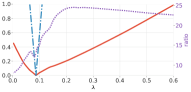
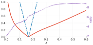
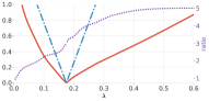
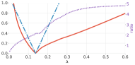
$s=7$

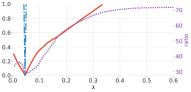
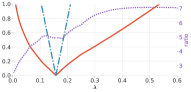
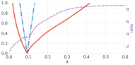
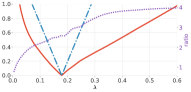
$s=15$

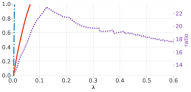
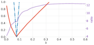
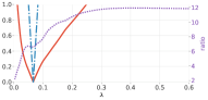
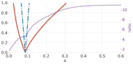
Figure 1: Lipschitzness of the solution mapping for $\lambda$ about $\bar{\lambda}:=\lambda^{*}$ as defined in Eq. 27. The red curve plots $\|\bar{x}(\lambda)-\bar{x}(\bar{\lambda})\|$; the blue curve, $|\lambda-\bar{\lambda}|\cdot\sqrt{s}/\sigma_{\min}(A_{I})^{2}$. The ratio of the two is given by the purple curve, whose $y$-axis is on the right side of each plot. From left to right, each column corresponds to $m=50,100,150,200$, respectively. See Table 1 for parameter settings and variable values.

The synthetic experiments were conducted for $s=3,7,15$ (corresponding to each row in the figure, respectively, top-to-bottom) and $m=50,100,150,200$ (corresponding to each column, respectively, left-to-right) with $N=200$. We selected $\gamma=0.1$ and for each $j\in\mathrm{supp}(x_{0}):=\{1,\ldots,s\}$, $(x_{0})_{j}=m+\sqrt{m}W_{j}$ where $W_{j}\overset{\text{iid}}{\sim}\mathcal{N}(0,1)$. Note that for each choice of $(s,m)$, $\lambda^{*}$ was chosen as the empirically best choice of tuning parameter from a logarithmically spaced grid of 501 $\lambda$ values approximately centered about a nearly asymptotically order-optimal choice $\gamma\sqrt{2\log n}$. The LASSO program was solved in Python using lasso_path from scikit-learn [48].

In Table 1 we report parameter values and relevant quantities associated with Fig. 1. In particular, the upper bound on the Lipschitz constant is given by $L:=\sqrt{s_{\lambda^{*}}}\cdot\sigma_{\min}^{-2}(A_{I})$. In essence, the quantity in the penultimate column determines whether Remark 4.1 holds (n.b., $A$ is a Gaussian random matrix, so $A_{I}$ has full rank almost surely when $|I|\leq m$). For all values of $s$ and $m$ in the experiment, $\|A_{I^{C}}(\bar{b}-A_{I}\bar{x}_{I})\|_{\infty}<\lambda^{*}$ (though we only present data up to three significant digits in Table 1). The only violation of Remark 4.1 was for $(s,m)=(15,50)$, for which $s_{\lambda^{*}}=63>m$ meaning $A_{I}$ was not of full column rank, violating condition (i). Successful recovery failed in this case, as discussed below.

$s$	$m$	$N$	$\eta$	$s_{\lambda^{*}}$	$L$00	$\sigma_{\min}(A_{I})$	$\|A_{I^{C}}(\bar{b}-A_{I}\bar{x}_{I})\|_{\infty}$	$\lambda^{*}$
3	50	200	0.1	25	43.5	0.339	0.0831	0.0866
3	100	200	0.1	22	15.4	0.552	0.162	0.167
3	150	200	0.1	20	10.2	0.661	0.175	0.175
3	200	200	0.1	20	8.23	0.737	0.136	0.137
7	50	200	0.1	41	236	0.165	0.0458	0.046
7	100	200	0.1	26	18.7	0.522	0.155	0.158
7	150	200	0.1	43	25.9	0.503	0.0931	0.0939
7	200	200	0.1	23	9.24	0.720	0.175	0.179
15	50	200	0.1	63	301	0.162	0.00322	0.00326
15	100	200	0.1	47	49.4	0.372	0.078	0.0781
15	150	200	0.1	66	62.5	0.361	0.0655	0.0665
15	200	200	0.1	67	46.2	0.421	0.085	0.0876

Table 1: Parameter settings corresponding with Figure 1. The assumption
$\|A_{I^{C}}(\bar{b}-A_{I}\bar{x}_{I})\|_{\infty}<\lambda^{*}$ is satisfied for all entries where $\lambda^{*}$ is defined as in Eq. 27 (n.b., the two entries in the third row only appear equal due to rounding error).

In every panel of the figure, the dash-dot curve is indeed a strict (local) upper bound on $\|\bar{x}(\lambda)-\bar{x}(\lambda^{*})\|$, supporting our theory. As predicted by the theory, the error $\|\bar{x}(\lambda)-\bar{x}(\lambda^{*})\|$ is more pronounced when the problem is under-regularized ($\lambda<\lambda^{*}$), and when the support size grows. Note that the $(s,m)=(15,50)$ plot (lower-left panel in the figure) corresponds to an unsuccessful approximate recovery of the ground truth signal $x_{0}$, due to the relatively large sparsity as compared to the number of measurements. In this setting, the small value of $\sigma_{\min}(A_{I})$ and the apparently poor behaviour of $\|\bar{x}(\lambda)-\bar{x}(\lambda^{*})\|$ is consistent with our theory. Similarly, the $(s,m)=(7,50)$ plot (middle-left panel in the figure) corresponds with a small value of $\sigma_{\min}(A_{I})$ due to the relatively small value of $m$ (and incidentally, it corresponds with poor recovery of the ground truth). Again, the relatively poor behaviour of $\|\bar{x}(\lambda)-\bar{x}(\lambda^{*})\|$ (as compared, say, with $m\geq 100$) is consistent with our theory.

6 Final remarks

In this paper we studied the optimal value and the optimal solution function of the LASSO problem as a function of both the right-hand side (or vector of measurements) $b\in\mathbb{R}^{m}$ and the regularization (or tuning) parameter $\lambda>0$. Our analysis of the optimal value function is based on classical convex analysis, while the study of the optimal solution function is based on modern variational analysis (in particular, differentiation of set-valued maps). As a by-product we established the (strong) metric regularity of the subdifferential of the objective function at a solution. The assumptions needed to perform this analysis were inspired by uniqueness results in the literature, and are shown to hold, e.g., in the case where the right-hand side at the point in question admits an irreducible sparse representation with respect to the columns of the measurement matrix. We then combined these variational-analytic findings with random matrix-theoretic arguments to study the sensitivity of the LASSO solution with respect to the tuning parameter, providing upper bounds for the corresponding Lipschitz constant that hold with high probability for measurement matrices of subgaussian type.

Several questions arise naturally as a topic of future research. Can analogous statements to Theorem 4.15 be proved for alternative formulations of $\ell_{1}$ minimization such as the constrained LASSO, quadratically-constrained basis pursuit, or the square-root LASSO? Similarly, the extension of our analysis to convex regularizers beyond the $\ell_{1}$-norm is an interesting open issue. In particular, can the analysis carried out here be generalized to the matrix setting with the nuclear norm in place of the $\ell_{1}$-norm? This will certainly require a good handle on the graph of the subdifferential of the nuclear norm. Finally, Example 4.22 suggests that the Lipschitz bound with respect to $\lambda$ provided by Corollary 4.20 might be hard to improve in general. Regarding applications to compressed sensing, another open problem is understanding whether our analysis could lead to results pertaining to the robustness to noise in the measurements.

Appendix A Supplement to Section 4

In this section provide some skipped proofs and further details on the results for the solution map of LASSO.

We commence with a fact that was employed to conclude the proof of Lemma 4.5. It was implicitly used that, given $z=(x,\|x\|_{1})$, then there is a one-to-one correspondence between the active set $\mathcal{A}(z)$ for $z\in\Omega:=\operatorname{epi}\|\cdot\|_{1}$ and $\mathrm{supp}(x)$. To this end, we realize that we can write the polyhedron $\Omega$ in the form

$$\Omega=\left\{(x,\alpha)\in\mathbb{R}^{n+1}\,\left|\;\binom{a^{\nu}}{-1}^{T}\binom{x}{\alpha}\leq 0\;(\nu\in\Lambda)\right.\right\}$$

for some finite index set $\Lambda$, such that the vectors $a^{\nu}$ are distinct and $a^{\nu}_{i}\in\{\pm 1\}$. Then $\nu$ is (by definition) an active index at $z$ if and only if $(a^{\nu})^{T}x=\|x\|_{1}$ which is the case if and only if

$$a_{\mathrm{supp}(x)}^{\nu}=\operatorname{sgn}(x_{\mathrm{supp}(x)}).$$

This shows the desired correspondence.

Next, we provide detailed calculations for Remark 4.19, in which $A$ is treated as a parameter of the solution map.

Remark A.1 (The matrix $A$ as a parameter).

Theorem 4.15 can be extended to the case where the solution is considered as a function of $(A,b,\lambda)$ by using analogous arguments. First, we consider the extended function $f:(\mathbb{R}^{m\times n}\times\mathbb{R}^{m}\times\mathbb{R}_{++})\times\mathbb{R}^{n}\to\mathbb{R}^{n}$ defined by $f(A,b,\lambda,x)=\frac{1}{\lambda}\left(A^{T}(Ax-b)\right)$, where, in this case, $\mathbb{R}^{m\times n}$ is equipped with the Frobenius norm $\|\cdot\|_{F}$. Similar to the proof of Theorem 4.15, we write $f((A,b,\lambda),x)=f(A,b,\lambda,x)$ and make an analogous abuse of notation for functions depending on both the parameters $(A,b,\lambda)$ and the variable $x$. First, a direct computation (e.g., see [43]) shows that

$$D_{A}f(\bar{A},\bar{b},\bar{\lambda},\bar{x})H=\bar{\lambda}^{-1}((\bar{A}^{T}H+H^{T}\bar{A})\bar{x}-H^{T}\bar{b}),$$

for any $H\in\mathbb{R}^{m\times n}$. We now show how to generalize the proof of Theorem 4.15 (a) by highlighting where its arguments need some modifications. The proof of the local Lipschitz continuity of the solution map $S:(A,b,\lambda)\mapsto\mathop{{\rm argmin}}_{x\in\mathbb{R}^{n}}\frac{1}{2}\|Ax-b\|^{2}+\lambda\|x\|_{1}$ is identical. Defining $G(A,b,\lambda,x)=f(A,b,\lambda,x)+F(x)$ and applying Proposition 4.11 and Lemma 2.3, we see that $DS(\bar{A},\bar{b},\bar{\lambda},\bar{x})$ is single-valued and locally Lipschitz with

$$DS(\bar{A},\bar{b},\bar{\lambda})(H,q,\alpha)=\left\{w\in\mathbb{R}^{n}\,\left|\;0\in DG(\bar{A},\bar{b},\bar{\lambda},\bar{x}|0)(H,q,\alpha,w)\right.\right\},$$

and where, thanks to Lemma 2.3,

$$DG(\bar{A},\bar{b},\bar{\lambda},\bar{x}|0)(H,q,\alpha,w) =\frac{1}{\bar{\lambda}}\left(\xi-{\bar{A}}^{T}\left(q+\frac{\alpha}{\bar{\lambda}}(\bar{A}\bar{x}-\bar{b})-\bar{A}w\right)\right)$$

$$+D(\partial\|\cdot\|_{1})(\bar{x}|-{\bar{A}}^{T}(\bar{A}\bar{x}-\bar{b}))(w),$$

where $\xi=\xi(\bar{A},\bar{b},\bar{x},H):=(\bar{A}^{T}H+H^{T}\bar{A})\bar{x}-H^{T}\bar{b}\in\mathbb{R}^{n}$. Arguing as in the proof of Theorem 4.15, we obtain

$$0 \in DG(\bar{A},\bar{b},\bar{\lambda},\bar{x}|0)(H,q,\alpha,w)$$

$$\implies\begin{cases}w_{I^{C}_{<}}=0\\ \bar{A}_{I}^{T}\left(q+\frac{\alpha}{\bar{\lambda}}(\bar{A}\bar{x}-\bar{b})-\bar{A}w\right)+\xi_{I}=0\\ w_{i}\left(\bar{A}_{i}^{T}\left(q+\frac{\alpha}{\bar{\lambda}}(\bar{A}\bar{x}-\bar{b})-\bar{A}w\right)+\xi_{i}\right)=0,\;\forall i\in I_{=}^{C}.\end{cases}$$

This, in turn, leads to the formula

$$S^{\prime}(\bar{A},\bar{b},\bar{\lambda})(H,q,\alpha)=L_{K}\left(({\bar{A}}_{K}^{T}\bar{A}_{K})^{-1}\left({\bar{A}}_{K}^{T}q+\frac{\alpha}{\bar{\lambda}}{\bar{A}}^{T}_{K}(\bar{A}\bar{x}-\bar{b})+\xi_{K}\right)\right).$$

Arguing again as in the proof of Theorem 4.15, observing that the function $\sigma_{\max}(\cdot)$ is continuous, and choosing a sequence $(A_{k},b_{k},\lambda_{k})\to(A,b,\lambda)$ such that $(A_{k})_{K}$ has full column rank for every $k\in\mathbb{N}$ (by passing to a subsequence if necessary), we see that there exists $(\bar{H},\bar{q},\bar{\lambda})\in\mathbb{B}$ such that

$$L \leq\frac{1}{\sigma_{\min}(\bar{A}_{K})^{2}}\left\|\bar{A}_{K}^{T}\bar{q}+\frac{\bar{\alpha}}{\bar{\lambda}}\bar{A}_{K}^{T}(\bar{A}\bar{x}-\bar{b})-(\bar{A}_{K}^{T}\bar{H}+\bar{H}_{K}^{T}\bar{A})\bar{x}+\bar{H}_{K}^{T}\bar{b}\right\|$$

$$\leq\frac{1}{\sigma_{\min}(\bar{A}_{K})^{2}}\left(\sigma_{\max}(\bar{A}_{K})+\left\|\frac{\bar{A}_{J}^{T}(\bar{A}\bar{x}-\bar{b})}{\bar{\lambda}}\right\|+\max_{\|H\|_{F}\leq 1}\left\|\bar{A}_{K}^{T}H\bar{x}+H_{K}^{T}(\bar{A}\bar{x}-\bar{b})\right\|\right)$$

$$\leq\frac{1}{\sigma_{\min}(\bar{A}_{K})^{2}}\left(\sigma_{\max}(\bar{A}_{K})+\left\|\frac{\bar{A}_{J}^{T}(\bar{A}\bar{x}-\bar{b})}{\bar{\lambda}}\right\|+\sigma_{\max}(\bar{A}_{K})\|\bar{x}\|+\|\bar{A}\bar{x}-\bar{b}\|\right)$$

$$\leq\frac{1}{\sigma_{\min}(\bar{A}_{J})^{2}}\left(\sigma_{\max}(\bar{A}_{J})(1+\|\bar{x}\|)+\left\|\frac{\bar{A}_{J}^{T}(\bar{A}\bar{x}-\bar{b})}{\bar{\lambda}}\right\|+\|\bar{A}\bar{x}-\bar{b}\|\right)$$

The extension of Theorem 4.15 (b) follows by analogous arguments, with $J=I$. $\diamond$

Appendix B Supplement to Section 5

We include here technical background from high-dimensional probability, which is required to prove Propositions 5.3 and 5.6. We state the result Lemma B.6 in a form similar to [55, Theorem 9.1.1] and moreover using the optimal dependence on $\beta$ established in [30]. For integers $1\leq s\leq n$, recall the definition of $\Sigma_{s}^{n}:=\{x\in\mathbb{R}^{n}:\|x\|_{0}\leq s\}$. In addition, let $T_{n,s}:=\sqrt{s}\mathbb{B}_{1}\cap\mathbb{B}_{2}$ and $J_{n,s}:=\mathrm{conv}\,(\Sigma_{s}^{n}\cap\mathbb{B}_{2})$. Throughout we let $\mathcal{C}\in\{J_{n,s},T_{n,s}\}$.

Definition B.1 (Restricted Isometry Property).

Let $0<\alpha_{-}\leq 1\leq\alpha_{+}<\infty$ and $s\in\mathbb{N}$. A matrix $A\in\mathbb{R}^{m\times n}$ satisfies the Restricted Isometry Property (RIP) of order $s$ with parameters $(\alpha_{-},\alpha_{+})$ if

$$\alpha_{-}\|x\|\leq\|Ax\|\leq\alpha_{+}\|x\|,\qquad\forall x\in\Sigma_{s}^{n}.$$

B.1 Matrix deviation inequalities

Next we introduce two auxiliary results that will be useful in establishing our results. The first is [30, Corollary 1.2].

Lemma B.2 ([30, Corollary 1.2]).

Let $A\in\mathbb{R}^{m\times n}$ be a $\beta$-subgaussian matrix and let $T\subseteq\mathbb{R}^{n}$ be a bounded set. Then

$$\operatorname{\mathbb{E}}\sup_{x\in T}\left|\|Ax\|-\sqrt{m}\|x\|\right|\leq C\beta\sqrt{\log\beta}\left[\operatorname{w}(T)+\operatorname{rad}(T)\right],$$

and for any $u\geq 0$, with probability at least $1-3e^{-u^{2}}$,

$$\sup_{x\in T}\left|\|Ax\|-\sqrt{m}\|x\|\right|\leq C\beta\sqrt{\log\beta}\left[\operatorname{w}(T)+u\cdot\operatorname{rad}(T)\right].$$

Here, $C>0$ is an absolute constant.

Above, $\operatorname{rad}T:=\sup_{x\in T}\|x\|$ and $\operatorname{w}(T)$ is the Gaussian mean width of a set $T\subseteq\mathbb{R}^{n}$:

$$\operatorname{w}(T):=\operatorname{\mathbb{E}}\sup_{x\in T}\left\langle x,\,g\right\rangle,\qquad\text{where}\;g_{i}\overset{\text{iid}}{\sim}\mathcal{N}(0,1),\quad i=1,\ldots,n.$$

Observe that $\operatorname{w}(T)=\operatorname{w}(\operatorname{conv}T)$, where $\operatorname{conv}T$ denotes the convex hull of $T$. We now summarize [55, Exercises 10.3.8–9] in the following lemma.

Lemma B.3 ([55, Exercises 10.3.8–9]).

For $C\geq c>0$ being absolute constants,

$$c\sqrt{s\log(2n/s)}\leq\operatorname{w}(J_{n,s})\leq\operatorname{w}(T_{n,s})\leq 2\operatorname{w}(J_{n,s})\leq C\sqrt{s\log(en/s)}.$$

The following lemma specializes [30, Corollary 1.2] using [55, Exercises 10.3.8–9].

Lemma B.4 (Sparse subgaussian deviations).

Let $A\in\mathbb{R}^{m\times n}$ be a $\beta$-subgaussian matrix and let $\mathcal{C}$ be either $J_{n,s}$ or $T_{n,s}$. For an appropriate choice of absolute constant $C>0$, it holds that

$$\operatorname{\mathbb{E}}\sup_{x\in\mathcal{C}}\left|\|Ax\|-\sqrt{m}\|x\|\right|\leq C\beta\sqrt{\log\beta}\left[\sqrt{s\log(en/s)}+1\right]$$

and for any $u\geq 0$, with probability at least $1-3e^{-u^{2}}$,

$$\sup_{x\in\mathcal{C}}\left|\|Ax\|-\sqrt{m}\|x\|\right|\leq C\beta\sqrt{\log\beta}\left[\sqrt{s\log(en/s)}+u\right].$$

Proof B.5 (Proof of Lemma B.4).

We demonstrate the proof for the expectation expression, since the probability bound follows by an identical set of steps. Combine Lemma B.2 and Lemma B.3 to obtain

$$\operatorname{\mathbb{E}}\sup_{x\in\mathcal{C}}\left|\|Ax\|-\sqrt{m}\|x\|\right|\leq C_{1}\beta\sqrt{\log\beta}\left[C_{2}\sqrt{s\log(en/s)}+1\right],$$

noting that $\operatorname{rad}\mathcal{C}=\sup_{x\in\mathcal{C}}\|x\|=1$. Above, we write $C_{1}$ to denote the absolute constant from [30, Corollary 1.2] and $C_{2}$ the one from [55, Exercise 10.3.8]. We obtain

$$C_{1}\beta\sqrt{\log\beta}\left[C_{2}\sqrt{s\log(en/s)}+1\right]\leq C\beta\sqrt{\log\beta}\left[\sqrt{s\log(en/s)}+1\right],$$

where $C:=C_{1}\max\{C_{2},1\}$ is the absolute constant appearing in the result statement, completing the proof.

B.2 Bounding singular values of submatrices

Finally, we present a probabilistic bound on the singular values of certain families of $s$-column submatrices, which in turn establishes a restricted isometry result for the class of matrices considered in section 5.1.

Lemma B.6.

Let $1\leq s\leq m\leq n$ be integers and let $\delta\in(0,1)$. Suppose that

$$m\geq C\delta^{-2}\beta^{2}\log\beta\left[s\log(en/s)+\log(3/\varepsilon)\right],$$

where $C>0$ is an absolute constant. If $A\in\mathbb{R}^{m\times n}$ is a normalized $\beta$-subgaussian matrix then with probability at least $1-\varepsilon$ on the realization of $A$ it holds that

$$1-\delta\leq\min_{|K|\leq s}\sigma_{\min}(A_{K})\leq\max_{|K|\leq s}\sigma_{\max}(A_{K})\leq 1+\delta.$$

In particular, $A$ satisfies RIP of order $s$ with parameters $(1-\delta,1+\delta)$.

Proof B.7 (Proof of Lemma B.6).

Let $\tilde{C}>0$ be the absolute constant from Lemma B.4 and set $C:=2\tilde{C}^{2}$. Recall that in Lemma B.4, $\mathcal{C}$ could have been either $J_{n,s}$ or $T_{n,s}$. Choose $\mathcal{C}:=J_{n,s}$. For $\delta$ as given in the result statement, if $m\geq 2\tilde{C}^{2}\delta^{-2}\beta^{2}\log\beta\left[s\log(en/s)+\log(3/\varepsilon)\right]$ and $A\in\mathbb{R}^{m\times n}$ is a normalized $\beta$-subgaussian matrix (i.e.,there exists a $\beta$-subgaussian matrix $\tilde{A}\in\mathbb{R}^{m\times n}$ with $A=m^{-1/2}\tilde{A}$), then, by Lemma B.4 with $u:=\sqrt{\log(3/\varepsilon)}$, it holds with probability at least $1-\varepsilon$ that

$$\sup_{x\in J_{n,s}}\left|\|Ax\|-\|x\|\right| \leq\frac{\tilde{C}\beta\sqrt{\log\beta}\left[\sqrt{s\log(en/s)}+\sqrt{\log(3/\varepsilon)}\right]}{\sqrt{m}}$$

$$\leq\delta\frac{\sqrt{s\log(en/s)}+\sqrt{\log(3/\varepsilon)}}{\sqrt{2}\cdot\sqrt{s\log(en/s)+\log(3/\varepsilon)}}$$

$$\leq\delta.$$

The first inequality is a consequence of the referenced result; the second obtained by substituting for $m$ and simplifying. The last line follows by an application of Jensen’s inequality (i.e., for $a,b\geq 0$ it holds that $\sqrt{2}\cdot\sqrt{a+b}\geq\sqrt{a}+\sqrt{b}$).

Restricting to $x\in J_{n,s}\cap\mathbb{S}^{{n}-1}$ thereby yields $\sup_{x\in J_{n,s}\cap\mathbb{S}^{{n}-1}}\left|\|Ax\|-1\right|\leq\delta$. In particular,

$$1-\delta\leq\|Ax\|\leq 1+\delta,\qquad\forall x\in J_{n,s}\cap\mathbb{S}^{{n}-1}.$$

Using positive homogeneity of $\|\cdot\|$, it follows that

(28) $$(1-\delta)\|x\|\leq\|Ax\|\leq(1+\delta)\|x\|,\qquad\forall x\in J_{n,s}.$$

It follows that, for any $K\subseteq\{1,\ldots,n\}$ with $|K|\leq s$,

$$(1-\delta)\|x\|\leq\|A_{K}x\|\leq(1+\delta)\|x\|,\qquad\forall x\in\mathbb{R}^{|K|}.$$

Specifically, Eq. 28 gives the desired result in view of the definition of $J_{n,s}$:

$$\sup_{x\in J_{n,s}\cap\mathbb{S}^{{n}-1}}\left|\|Ax\|-1\right|\leq\delta$$

$$\implies\quad\sup_{|K|\leq s}\sup_{x\in\mathbb{S}^{{|K|}-1}}\left|\|A_{K}x\|-1\right|\leq\delta$$

$$\implies\quad(1-\delta)\leq\|A_{K}x\|\leq(1+\delta),\qquad\forall K\subseteq\{1,\ldots,n\}\;\text{with}\;|K|\leq s,\quad\forall x\in\mathbb{S}^{{|K|}-1}$$

$$\implies\quad 1-\delta\leq\min_{|K|\leq s}\sigma_{\min}(A_{K})\leq\max_{|K|\leq s}\sigma_{\max}(A_{K})\leq 1+\delta.$$

(Note the final implication is obtained from one characterization of the extremal singular values of a matrix — see [55, (4.5)].) Clearly $A$ satisfies RIP of order $s$ with parameters $(1-\delta,1+\delta)$ in view of Definition B.1.

References

- [1] B. Adcock, A. Bao, and S. Brugiapaglia: Correcting for unknown errors in sparse high-dimensional function approximation. Numerische Mathematik 142(3), 2019, pp. 667–711.
- [2] B. Adcock and A.C. Hansen: Compressive Imaging: Structure, Sampling, Learning. Cambridge University Press, Cambridge, UK, 2021.
- [3] F.J. Aragón Artacho and M.H. Geoffroy: Characterization of metric regularity of subdifferentials. Journal of Convex Analysis 15(2), 2008, pp. 365–380.
- [4] H. Bauschke and P.L. Combettes: Convex analysis and monotone operator theory in Hilbert spaces. Springer, New York, USA, 2011.
- [5] M. Bayati and A. Montanari: The Lasso risk for Gaussian matrices. IEEE Transactions on Information Theory 58(4), 2011, pp. 1997–2017.
- [6] A. Beck: First-Order Methods in Optimization. MOS-SIAM Series on Optimization, SIAM, Philadelphia, USA, 2017.
- [7] Y. Bello-Cruz, G. Li, T.T. An Nghia: Quadratic growth conditions and uniqueness of optimal solution to Lasso. Journal of Optimization Theory and Applications, 194, 2022, pp. 167–190.
- [8] A. Berk: On LASSO parameter sensitivity. University of British Columbia, 2021. (Ph.D. thesis)
- [9] A. Berk, Y. Plan, and Ö. Yilmaz: Sensitivity of minimization to parameter choice. Information and Inference: A Journal of the IMA 10(2), 2021, pp. 397–453.
- [10] A. Berk, Y. Plan, and Ö. Yilmaz: On the best choice of LASSO program given data parameters. IEEE Transactions on Information Theory 68(4), 2022, pp. 2573–2603.
- [11] A. Beck and M. Teboulle: A fast iterative shrinkage-thresholding algorithm for linear inverse problems. SIAM Journal of Imaging Sciences 2(1), 2009, pp. 183–202.
- [12] P.J. Bickel, Y. Ritov, and A.B. Tsybakov: Simultaneous analysis of Lasso and Dantzig selector. The Annals of Statistics, 37(4), 2009, pp. 1705–1732.
- [13] J.F. Bonnans and A. Shapiro: Perturbation Analysis of Optimization Problems. Springer Series in Operations Research. Springer, New York, 2000.
- [14] J.V. Burke and J.J. Moré: On the identificiation of active constraints. SIAM Journal on Numerical Analysis 25(5), 1988, pp. 1198–1211.
- [15] E.J. Candès, J. Romberg, and T. Tao: Stable signal recovery from incomplete and inaccurate measurements. Communications on Pure and Applied Mathematics 59, 2006, pp. 1207–1223.
- [16] E.J. Candès, and T. Tao: Decoding by linear programming. IEEE Transactions on Information Theory 51(12), 2005, pp. 4203–4215.
- [17] S.S. Chen, D.L. Donoho, and M.A. Saunders: Atomic decomposition by basis pursuit. SIAM Journal on Scientific Computing 2(1), 1998, pp. 33–61.
- [18] D.L. Donoho: Compressed sensing IEEE Transactions on information theory 52(4), 2006, pp. 1289–1306.
- [19] A.L. Dontchev and R.T. Rockafellar: Implicit Functions and Solution Mappings: a View from Variational Analysis, 2nd Edition. Springer Series in Operations Research and Financial Engineering. Springer, New York, Heidelberg, Dordrecht, London, 2014.
- [20] Y.C. Eldar and G. Kutyniok, eds: Compressed Sensing: Theory and Applications. Cambridge University Press, Cambridge, UK, 2012.
- [21] M.P. Friedlander, A. Goodwin, and T. Hoheisel: From perspective maps to epigraphical projections. Mathematics of Operations Research, 2022 (doi.org/10.1287/moor.2022.1317).
- [22] S. Foucart and H. Rauhut: A Mathematical Introduction to Compressive Sensing. Applied and Numerical Harmonic Analysis, Birkhäuser, New York, NY, 2013.
- [23] S. Foucart, E. Tadmor, and M. Zhong: On the sparsity of LASSO minimizers in sparse data recovery. arXiv:2004.04348, 2020.
- [24] S. Foucart: The sparsity of LASSO-type minimizers. Applied and Computational Harmonic Analysis, 62, 2023, pp. 441-–452.
- [25] J.-J. Fuchs: On sparse representations in arbitrary redundant bases. IEEE Transactions on Information Theory 50(6), 2004, pp. 1341–1344.
- [26] T. Hastie, R. Tibshirani, and M. Wainwright: Statistical Learning with Sparsity. Chapman and Hall/CRC, New York, NY, 2015.
- [27] J.C. Gilbert: On the solution uniqueness characterization in the L1 norm and polyhderal gauge recovery. Journal of Optimization Theory and Applications 172, 2017, pp. 70–101.
- [28] T. Hoheisel: Topics in Convex Analysis in Matrix Space. Lecture Notes, Spring School on Variational Analysis, Paseky nad Jizerou, Czech Republic, 2019.
- [29] R. Horn and C.R. Johnson: Matrix Analysis. Cambridge University Press, Cambridge, 2nd Edition, 2013.
- [30] H. Jeong, X. Li, Y. Plan, and Ö. Yilmaz: Sub-gaussian matrices on sets: optimal tail dependence and applications. Communications on Pure and Applied Mathematics, 75(8), 2022, pp. 1713–1754.
- [31] C. Kanzow and T. Lechner: Globalized inexact proximal Newton-type methods for nonconvex composite functions. Computational Optimization and Applications 78, 2021, pp. 377–410.
- [32] P.D. Khanh, B.S. Mordukhovich, and V.T. Phat: A generalized Newton method for subgradient systems. arXiv:2009.10551, 2021.
- [33] M.-J. Lai and Y. Wang: Sparse Solutions of Underdetermined Linear Systems and Their Applications. Society for Industrial and Applied Mathematics, Philadelphia, PA, 2021.
- [34] J.D. Lee, Y. Sun, and M.A. Saunders: Proximal Newton-type methods for minimizing composite functions. SIAM Journal on Optimization 24(3), 2014, pp. 1420–1443.
- [35] A.S. Lewis: Active Sets, nonsmoothness, and sensitivity. SIAM Journal on Optimization 13(3), 2002, pp. 702–725.
- [36] A. Milzarek and M. Ulbrich: A semismooth Newton method with multidimensional filter globalization for -optimization. SIAM Journal on Optimization 24, 2014, pp. 298–333.
- [37] B.S. Mordukhovich: Variational Analysis and Generalized Differentiation. I: Basic Theory. Grundlehren Series (Fundamental Principles of Mathematical Sciences), Vol. 330, Springer, Berlin, 2006.
- [38] B.S. Mordukhovich: Variational Analysis and Applications. Springer Monographs in Mathematics book series, Springer International Publishing AG, 2018.
- [39] B.K. Natarajan: Sparse approximate solutions to linear systems. SIAM Journal on Computing 24, 1995, pp. 227–234.
- [40] J. Nocedal and S.J. Wright: Numerical Optimization (Second Edition). Springer Series in Operations Research and Financial Engineering, Springer, New York, 2006.
- [41] S. Oymak, C. Thrampoulidis, and B. Hassibi: The squared-error of generalized Lasso: a precise analysis. In 2013 51st Annual Allerton Conference on Communication, Control, and Computing (Allerton), 2013, pp. 1002–1009.
- [42] T. Park and G. Casella: The Bayesian Lasso. Journal of the American Statistical Association 103(482), 2008, pp. 681–686.
- [43] K.B. Petersen and M.S. Pedersen: The matrix cookbook. Technical University of Denmark, ver. 20121115, 2018.
- [44] R.T. Rockafellar: Convex Analysis. Princeton Mathematical Series, No. 28. Princeton University Press, Princeton, NJ, 1970.
- [45] R.T. Rockafellar and R.J.-B. Wets: Variational Analysis. Grundlehren der Mathematischen Wissenschaften, Vol. 317, Springer-Verlag, Berlin, 1998.
- [46] F. Santosa and W.W. Symes: Linear inversion of band-limited reflection seismograms. SIAM Journal on Scientific and Statistical Computing 7(4), 1986, pp. 1307–1330.
- [47] Y. Shen, B. Han, and E. Braverman: Stable recovery of analysis based approaches. Applied and Computational Harmonic Analysis, 39(1), 2015, pp. 161–172.
- [48] F. Pedregosa, G. Varoquaux, A. Gramfort, V. Michel, B. Thirion, O. Grisel, et al.: Scikit-learn: Machine learning in Python. The Journal of machine Learning research, 12, 2011, pp. 2825–2830.
- [49] C. Thrampoulidis, A. Panahi, and B. Hassibi: Asymptotically exact error analysis for the generalized -Lasso. In 2015 IEEE International Symposium on Information Theory (ISIT), 2015, pp. 2021–2025.
- [50] C. Thrampoulidis, E. Abbasi, and B. Hassibi: Precise error analysis of regularized -estimators in high dimensions. IEEE Transactions on Information Theory, 64(8), 2018, pp. 5592–5628.
- [51] R.J. Tibshirani: Regression shrinkage and selection via the lasso. Journal of the Royal Statistic Society (Series B) 58, 1996, pp. 267–288.
- [52] R.J. Tibshirani: The lasso problem and uniqueness. Electronic Journal of Statistics 7, 2013, pp. 1456–1490.
- [53] S. Vaiter, G. Peyré, and J. Fadili: Low complexity regularization of linear inverse problems. In: Sampling Theory, a Renaissance. Ed. G.E. Pfander, Applied and Numerical Harmonic Analysis, Birkhäuser/Springer, Cham, 2015, pp. 103–153.
- [54] S. Vaiter, C. Deledalle, J. Fadili, G. Peyré, and C. Dossal: The degrees of freedom of partly smooth regularizers. Annals of the Instutute of Statistical Mathematics, 69, 2017, pp. 791–832.
- [55] R. Vershynin:High-Dimensional Probability: an Introduction with Applications in Data Science. Cambridge University Press, Cambridge, UK, 2017.
- [56] M. Vidyasagar: An introduction to compressed sensing. Society for Industrial and Applied Mathematics, Philadelphia, NY, 2019.
- [57] M.J. Wainwright: High-dimensional statistics: A non-asymptotic viewpoint. Cambridge University Press, Cambridge, UK, 2019.
- [58] H. Zhang, W. Yin, and L. Cheng: Necessary and sufficient conditions of solution uniqueness in -norm minimization. Journal of Optimization Theory and Applications, 164, 2015, pp. 109–122.