Semiparametric Gaussian Copula Regression modeling for Mixed Data Types (SGCRM)

Abstract

Many clinical and epidemiological studies encode collected participant-level information via a collection of continuous, truncated, ordinal, and binary variables. To gain novel insights in understanding complex interactions between collected variables, there is a critical need for the development of flexible frameworks for joint modeling of mixed data types variables. We propose Semiparametric Gaussian Copula Regression modeling (SGCRM) that allows to model a joint dependence structure between observed continuous, truncated, ordinal, and binary variables and to construct conditional models with these four data types as outcomes with a guarantee that derived conditional models are mutually consistent. Semiparametric Gaussian Copula (SGC) mechanism assumes that observed SGC variables are generated by i) monotonically transforming marginals of latent multivariate normal random variable and ii) dichotimizing/truncating these transformed marginals. SGCRM estimates the correlation matrix of the latent normal variables through an inversion of “bridges” between Kendall’s Tau rank correlations of observed mixed data type variables and latent Gaussian correlations. We derive a novel bridging result to deal with a general ordinal variable. In addition to the previously established asymptotic consistency, we establish asymptotic normality of the latent correlation estimators. We also establish the asymptotic normality of SGCRM regression estimators and provide a computationally efficient way to calculate asymptotic covariances. We propose computationally efficient methods to predict SGC latent variables and to do imputation of missing data. Using National Health and Nutrition Examination Survey (NHANES), we illustrate SGCRM and compare it with the traditional conditional regression models including truncated Gaussian regression, ordinal probit, and probit models.

Keywords: Joint modeling, Multivariate analysis, Mixed outcome

1 Introduction

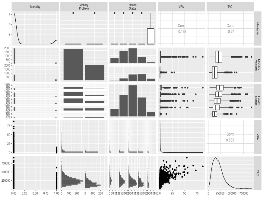
Figure S2: Exploratory analysis for our variables of interest from NHANES

Clinical and epidemiological studies as well as health surveys collect a large number of health outcomes, physiological and clinical measures encoded via a collection of continuous, truncated, ordinal, and binary variables. As a main motivating example, we consider National Health and Nutrition Examination Survey (NHANES), a cross-sectional, nationally representative survey that assesses dietary and health-related behaviours that can be used to better understand national trends in health and nutrition. Self-reported current health status (on scale 1-5, 1 = excellent, 2 = very good, 3 = good, 4 = fair, 5 = poor) is an example of the ordinal variable. Self-reported mobility problem (0/1 = no/yes for mobility difficulty) and 5-year follow-up mortality status (0/1 = alive/deceased at the 5-year follow-up) are examples of binary variables. In 2003-2006 waves, NHANES measured physical activity using accelerometry and summarized physical activity levels using two variables: Total Activity Count (TAC) and a time spent doing Vigorous Physical Activity (VPA). TAC is a continuous measure of the total volume of physical activity and VPA is a truncated measure of the high intensity physical activity as many, especially elderly, participants are not involved in high-intensity physical activity. Figure S2 show scatterplot matrix of these five variables. Several NHANES studies used these five variables as outcomes in linear regression models (TAC), truncated regression (VPA), ordinal regression (health status), and logistic regression models (mobility difficulty and mortality status) (Troiano et al., 2008; Wolff-Hughes et al., 2015; Varma et al., 2017; Leroux et al., 2019). Although, the results of those models are often aggregated in literature reviews, those models and potentially their results are not necessarily mutually consistent. Thus, to better understand interrelationships between health-related outcomes collected by studies such as NHANES, we need better tools for modeling dependency structures across mixed data types variables. Below, we review the current state of conditional and joint modeling for mixed data types and then discuss our contributions.

Due to a lack of standard joint models for multivariate mixed data types, conditional modeling is frequently used instead. Conditional models focus on choosing one of the variables as an outcome and modeling the conditional mean of this outcome as a function of other variables. Logistic and probit regressions are popular choice for a binary outcome. The cumulative ordinal regression model McCullagh (1980) is a popular choice for an ordinal outcome. For a truncated outcome, Tobit models, proposed in econometrics literature (Tobin, 1958; Heckman, 1976; Hausman & Wise, 1977), assume the outcome is generated via a truncation of a latent normal variable and the conditional mean of the latent variable is modeled as a linear function of the predictors. The Tobit model was generalized as the Hurdle model (Cragg, 1971), where conditional models are considered both for the truncated and non-truncated outcome separately at the cost of introducing more parameters. These models require likelihood-based numerical approaches and can suffer from convergence issues.

Factorization models combine both conditional and marginal distributions. A popular example is General Location models (GLOMs) (Olkin & Tate, 1961), which enforce conditional normality for continuous variables and arbitrary distribution for discrete components. Another example is conditional grouped conditional models (CGCMs) (Anderson & Pemberton, 1985; de Leon & Carriégre, 2007; De Leon, 2005) that assumes that the discrete variables are derived by truncating a latent multivariate continuous distribution. These models employs polychoric and polyserial correlations to estimate a joint covariance structure. Even though, factorization models provide a convenient way for specifying mixed distributions, they induce a hierarchy in the data that depend on the direction of conditioning. Different factorizations for the same set of variables can lead to different interpretations for the estimated parameters and different inferences for associations.

Another class is copula-based models. For example, (Song et al., 2009) defined Vector Generalized Linear Models (VGLMs) for modeling mixed data type outcomes. This approach requires embedding the marginal distributions (univariate Generalized Linear Models) into the joint distribution function via a Gaussian copula. Gaussian copulas is a popular choice to couple marginal distributions because of their analytical tractability and flexibility. Jiryaie et al. (2016) introduced Gaussian copula distributions (GCD) that take a latent variable approach to embed discrete variables using the Gaussian copula. However, CGCMs, GLOMs, VGLMs, and GCDs require likelihood-based inference and are computationally intensive for high dimensions. Pairwise likelihood-based approaches (De Leon, 2005; Jiryaie et al., 2016) reduce the computational burden but can make worse classification than the full likelihood-based approach (Jiryaie et al., 2016).

Recently, semiparametric models have seen a wide adaptation for joint modeling of multivariate mixed type data. Wang & Hua (2014) used likelihood-based inference and Cai & Zhang (2015) developed a rank-based approach to estimate a joint semiparametric Gaussian copula for continuous variables. Fan et al. (2016) extended the rank-based approaches to perform quantile regression on continuous variables. Rank-based estimation of the covariance of the semi-parametric Gaussian copula family (Liu et al., 2009, 2012) has been particularly attractive because of the fast and robust estimation procedure. In addition, multiple recent extensions used latent semi-parametric Gaussian copula to model mixed types data. Fan et al. (2017) developed the estimation for the case of binary and continuous variables. Yoon et al. (2018) extended the approach to include truncated variables, and Quan et al. (2018) has additionally extended it to include ternary variables (ordinal variables with three categories) and general ordinal-continuous pairs of variables. Feng & Ning (2019) represented an ordinal variable via multiple dummy binary variables and took a weighted correlation approach to recover the latent correlation for ordinal pairs with more than three categories. Whereas, Zhang et al. (2018) arrived at an incorrect bridging function trying to tackle the general ordinal case. Huang et al. (2021) provided an R package for speeding up numerical calculation of latent correlations between pairs of binary, ternary, truncated and continuous variables using a numerical interpolation approach.

Our main contributions are as follows. First, we fill the gap and provide the analytical bridging formulas for the case of a general ordinal variable. Second, we propose Semiparametric Gaussian Copula Regression modeling (SGCRM) framework for mutually consistent conditional modeling of mixed types outcomes. The approach is semi-parametric likelihood-free and computationally fast. To facilitate inference, we, first, obtain a novel result establishing asymptotic normality of SGC latent correlation estimators, and then, build on that and establish asymptotic normality of SGCRM regression estimators. Third, we derive computationally efficient algorithms for estimating SGC latent variables and imputation of missing variables within SGC mechanism. modeling advantages of SGRCM include: i) mutually consistent conditional modeling as an alternative to conditional models such as linear, probit and truncated regression, ii) a natural normalization of heterogeneous scales of mixed data types, iii) the regression results are monotone transformation invariant, iv) intuitive interpretation of the regression coefficients and comparison of the effect sizes based on $R^{2}$ on the latent space.

The rest of the paper is organized as follows. Chapter 2 reviews semiparametric Gaussian Copula model and demonstrates how to handle a general ordinal variable. Chapter 3 introduces Semiparametric Gaussian Copula Regression Model, derives novel asymptotical results, and describes key advantages of SGCRM. Chapter 4 covers two methodological applications of SGCRM: prediction of latent variables and imputation of missing observations. Chapter 5 studies the performance of SGCRM via multiple simulation scenarios. Chapter 6 illustrates SGCRM in NHANES. Finally, Chapter 7 concludes with a discussion.

2 Gaussian copula model

Classical Gaussian model assumptions have been popular due to their computational simplicity. However, these assumptions can be too restrictive. As an alternative, Liu et al. (2009) proposed non-Paranormal distribution (NPN) which can be seen as a semiparametric Gaussian Copula model.

Definition 2.1.

(Non-paranormal distribution) A random vector $Z=(Z_{1},\dots,Z_{p})^{\prime}\sim NPN_{p}(0,\Sigma,f)$, if there exist monotone transformation functions $f=(f_{1},...,f_{p})$ such that $L=(L_{1},\dots,L_{p})=f(Z)=(f_{1}(Z_{1}),\dots,f_{p}(Z_{p}))\sim N(0,\Sigma)$, where $\Sigma_{jj}=1$ for $1\leq j\leq p$.

The assumption on $\Sigma$ is made to ensure the identifiability of the distribution as shown in Liu et al. (2009).

Fan et al. (2017) introduced latent non-paranormal distribution which extended non-paranormal distribution to jointly model binary and continuous data. Yoon et al. (2018) introduced truncated variables using latent non-paranormal variables and Quan et al. (2018) extended the distribution to ternary-continuous pairs and ternary-ternary pairs. We generalize these results even further and treat a (general) ordinal ($k$ ordered categories) case. We define Generalized Latent Non-paranormal (GLNPN) distribution with four mixed data types including continuous, truncated, (general) ordinal ($k$ ordered categories), binary variables.

Definition 2.2.

(Generalized latent non-paranormal distribution) Suppose we observe a random vector $X=(X_{c},X_{t},X_{o},X_{b})^{\prime}$, where $X_{c}$ is $p_{c}$-dimensional continuous variable, $X_{t}$ is $p_{t}$-dimensional truncated, $X_{o}$ is $p_{o}$-dimensional ordinal ($j$-th ordinal variable has levels $\{0,1,\cdots,l_{j}-1\}$), and $X_{b}$ is $p_{b}$-dimensional binary variable, and $p=p_{c}+p_{t}+p_{o}+p_{b}$. We assume that there exist latent variables $Z=(Z_{c},Z_{t},Z_{o},Z_{b})^{\prime}$ such that

$$X_{cj} =Z_{cj},1\leq j\leq p_{c}$$ (1)

$$X_{tj} =Z_{tj}I(Z_{tj}>\delta_{tj}),1\leq j\leq p_{t}$$

$$X_{oj} =\sum_{k=0}^{l_{j}-1}kI(\delta_{ojk}\leq Z_{oj}<\delta_{oj(k+1)}),1\leq j\leq p_{o};\delta_{oj0}=-\infty,\delta_{ojl_{j}}=\infty$$

$$X_{bj} =I(Z_{bj}>\delta_{bj}),1\leq j\leq p_{b}$$

If $Z=(Z_{c},Z_{t},Z_{o},Z_{b})^{\prime}\sim NPN(0,\Sigma,f)$, we denote that $X=(X_{c},X_{t},X_{o},X_{b})^{\prime}\sim\mathrm{GLNPN}_{p}(0,\Sigma,f,\bm{\delta})$, where $\bm{\delta}=\{\delta_{tj};j=1,\cdots,p_{t}\}\cup(\cup_{j=1}^{p_{o}}\{\delta_{oj(k+1)};k=0,\cdots,l_{j}\})\cup\{\delta_{bj};j=1,\cdots,p_{b}\}$, i.e., is the set containing cutoffs for truncated, ordinal and binary variables.

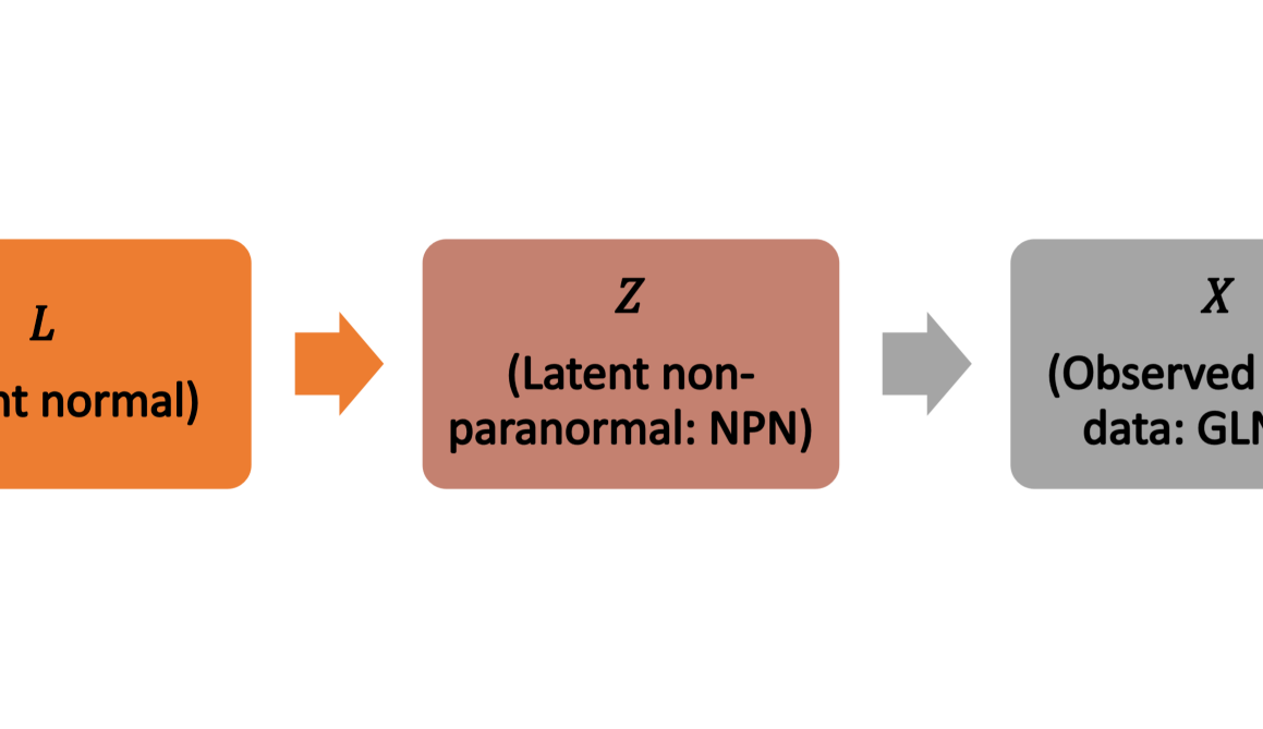
Figure 1: The data generation flow of GLNPN distribution

For notational simplicity, we will refer to observed continuous, truncated, ordinal, binary variables generated according to GLNPN distribution as CTOB-GLNPN variables. Figure 1 shows the flowchart of the data generation mechanism for observed GLNPN variables. Figure 2 shows an example of four observed CTOB-GLNPN variables generated via monotone-transformation-then-truncation of latent bivariate normal variables.

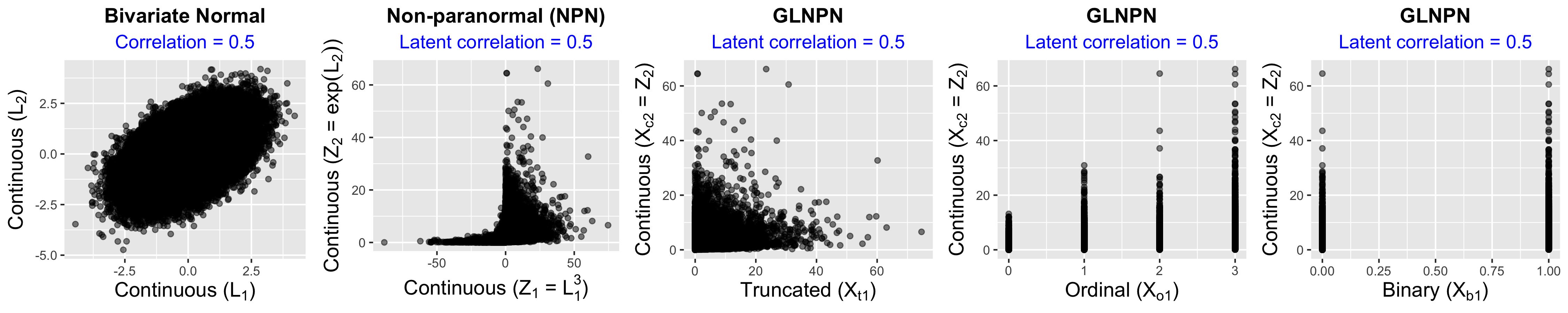
Figure 2: From left to right: (i) a scatterplot of bivariate standard normal variables with correlation of $0.5$, (ii) a continuous-continuous pair, (iii) a truncated-continuous pair, iv) an ordinal-continuous pair, (v) a binary-continuous pair

Cut-off parameters of GLNPN distribution suffers from identifiability issues (discussed in details at Fan et al. (2017)). The joint probability mass function of the discrete component or the density of the truncated component only depends on the set of transformed cutoffs: $\mathbf{\Delta}=f(\bm{\delta})=\{f_{j}(\delta_{tj});j=1,\cdots,p_{t}\}\cup(\cup_{j=1}^{p_{o}}\{f_{j}(\delta_{oj(k+1)});k=0,\cdots,l_{j}\})\\ \cup\{f_{j}(\delta_{bj});j=1,\cdots,p_{b}\}=\{\Delta_{tj};j=1,\cdots,p_{t}\}\cup(\cup_{j=1}^{p_{o}}\{\Delta_{oj(k+1)};k=0,\cdots,l_{j}\})\\ \cup\{\Delta_{bj};j=1,\cdots,p_{b}\}$. To emphasize this, we will generally refer to GLNPN distribution as $\mathrm{GLNPN}_{p}(0,\Sigma,f,\mathbf{\Delta})$.

As a result of the identifiablity constraints for the cutoffs, the binary and ordinal components of GLNPN distribution are marginally equivalent to the latent Gaussian distribution for binary and ordinal variables. This comes as no surprise as the discrete components does not have enough information to identify the marginal transformations. However, when we model the discrete component jointly with continuous and truncated variables, the class of GLNPN distributions becomes much larger than the class of latent Gaussian distributions (Yoon et al., 2018; Fan et al., 2017). The marginal transformations from continuous and truncated variables make the joint distribution of mixed variables more flexible and potentially can provide a substantial advantage to better explain the association between mixed type of variables.

2.1 Estimation of Correlation Matrix

2.1.1 Bridging functions

A few authors (including Fan et al. (2017); Yoon et al. (2018); Quan et al. (2018)) have considered Kendall’s $\tau$ rank correlation to estimate latent correlation matrix $\Sigma$ for different combinations of continuous, truncated, ternary, and binary variables. For two independent copies $X_{i}$, $X_{i}^{\prime}$ of the random vector $X$, the population-level Kendall’s $\tau$ is defined as

$$\tau_{jk}=E[sgn\{(X_{ij}-X_{i^{\prime}j})(X_{ik}-X_{i^{\prime}k})\}]$$ (2)

We can calculate a sample Kendall’s tau between $j$-th and $k$-th variable as follows:

$$\hat{\tau}_{jk}=\frac{2}{n(n-1)}\sum_{1\leq i<i^{\prime}<n}sgn\{(X_{ij}-X_{i^{\prime}j})(X_{ik}-X_{i^{\prime}k})\}$$ (3)

The construction of Kendall’s $\tau$ reveals that it is invariant under a monotone transformation.

Under GLNPN, the population-level Kendall’s Tau can be related to the latent correlation $\Sigma_{jk}$ through a one-to-one bridging function $F$ which for non-continuous components will depend on cutoffs as $\tau_{jk}=F(\Sigma_{jk})$. The estimated latent correlation is then obtained as $\hat{\Sigma}_{jk}=F^{-1}(\hat{\tau}_{jk})$.

Fan et al. (2017) calculated the bridging function for a pair of binary and continuous variables, Yoon et al. (2018) showed how to deal with truncated variables in addition to continuous and binary. Quan et al. (2018) provided formulas for bridging functions for ternary variables and for general ordinal-continuous pairs of variables. Feng & Ning (2019) broke an ordinal variable into multiple dummy binary variables and took a weighted correlation approach to recover the latent correlation for ordinal pairs with more than three categories, whereas, Zhang et al. (2018) arrived at an incorrect bridging function trying to tackle the general ordinal case. We summarize the references to the correct bridging functions for all possible pairs of variables in Table 1. Our first contribution is to derive bridging functions for the general ordinal variable with an arbitrary number of ordinal levels. We derive bridging functions for ordinal-truncated, ordinal-ordinal, and ordinal-binary pairs in Theorem 1 and prove the invertibility of the functions in Theorem 2.

Type	Continuous	Truncated	Ordinal∗	Binary
Continuous	Liu et al. (2009)	Yoon et al. (2018)	Quan et al. (2018)	Fan et al. (2017)
Truncated	Yoon et al. (2018)	Yoon et al. (2018)	Theorem 1	Yoon et al. (2018)
Ordinal	Quan et al. (2018)	Theorem 1	Theorem 1	Theorem 1
Binary	Fan et al. (2017)	Yoon et al. (2018)	Theorem 1	Fan et al. (2017)

Table 1: The reference of bridging functions for all possible pairs of variables.
^∗Ordinal cases for only three categories were derived in Quan et al. (2018)

For completeness, the following theorem also includes the previously established bridging functions.

Theorem 1.

Let $X_{j},X_{k}$ be two GLNPN variables, then the population Kendall’s Tau is related to the latent correlation as follows: $\tau_{jk}=F(\Sigma_{jk})$, where $F$ additionally depends on the cutoffs ${\Delta_{j}},{\Delta_{k}}$ for non-continuous components. The bridging functions corresponding to all pairs of variables are as follows

$$F_{\rm cc}(\rho) =\dfrac{2}{\pi}\sin^{-1}(\rho)$$

$$F_{\rm bb}(\rho;\Delta_{j},\Delta_{k}) =2\left\{\Phi_{2}(\Delta_{j},\Delta_{k};\rho)-\Phi(\Delta_{j})\Phi(\Delta_{k})\right\}$$

$$F_{\rm cb}(\rho;\Delta_{j}) =4\Phi_{2}(\Delta_{j},0;\rho/\sqrt{2})-2\Phi(\Delta_{j})$$

$$F_{\rm tb}(\rho;\Delta_{j},\Delta_{k}) =2\Phi_{3}\left(\Delta_{k},-\Delta_{j},0;S_{3a}(\rho)\right)-2\Phi_{3}\left(\Delta_{k},-\Delta_{j},0;S_{3b}(\rho)\right)$$

$$F_{\rm ct}(\rho;\Delta_{j}) =-2\Phi_{2}(-\Delta_{j},0;1/\sqrt{2})+4\Phi_{3}\left(-\Delta_{j},0,0;S_{3}(\rho)\right)$$

$$F_{\rm tt}(\rho;\Delta_{j},\Delta_{k}) =-2\Phi_{4}(-\Delta_{j},-\Delta_{k},0,0;S_{4a}(\rho))+2\Phi_{4}(-\Delta_{j},-\Delta_{k},0,0;S_{4b}(\rho))$$

$$F_{\rm co}(\rho;\Delta_{j}) =\sum_{r=1}^{l_{j}-1}(4\Phi_{3}(\Delta_{jr},\Delta_{j(r+1)},0)-2\Phi(\Delta_{jr})\Phi(\Delta_{j(r+1)}))$$

$$F_{\rm oo}(\rho;\Delta_{j},\Delta_{k}) =2\sum_{r=1}^{l_{j}-1}\sum_{s=1}^{l_{k}-1}[\Phi_{2}(\Delta_{jr},\Delta_{ks};\rho)\{\Phi_{2}(\Delta_{j(r+1)},\Delta_{k(s+1)};\rho)-\Phi_{2}(\Delta_{j(r+1)},\Delta_{k(s-1)};\rho)\}]-$$

$$2\sum_{r=1}^{l_{j}-1}\Phi({\Delta_{jr}})\Phi_{2}(\Delta_{j(r+1)},\Delta_{k(l_{k}-1)};\rho)$$ (4)

$$F_{\rm ob}(\rho;\Delta_{j},\Delta_{k}) =2\sum_{r=1}^{l_{j}-1}[\Phi_{2}(\Delta_{jr},\Delta_{k};\rho)\Phi(\Delta_{j(r+1)})-\Phi({\Delta_{jr}})\Phi_{2}(\Delta_{j(r+1)},\Delta_{k};\rho)]$$

$$F_{\rm to}(\rho;\Delta_{j},\Delta_{k}) =2\Phi_{3}((\Delta_{k(l_{k}-1)},-\Delta_{j},0);S_{3a}(\rho))-2\sum_{r=1}^{l_{j}-1}[\Phi_{4}((\Delta_{k(r+1)},\Delta_{kr},-\Delta_{j},0);S_{5}(\rho))-$$ (5)

$$\Phi_{4}((\Delta_{k(r-1)},\Delta_{kr},-\Delta_{j},0);S_{5}(\rho))]$$ (6)

with

$$\begin{split}S_{3a}(\rho)&=\begin{pmatrix}1&0&\frac{\rho}{\sqrt{2}}\\ 0&1&\frac{1}{\sqrt{2}}\\ \frac{\rho}{\sqrt{2}}&\frac{1}{\sqrt{2}}&1\end{pmatrix},\quad S_{3b}(\rho)=\begin{pmatrix}1&0&-1/\sqrt{2}\\ 0&1&-\rho/\sqrt{2}\\ -1/\sqrt{2}&-\rho/\sqrt{2}&1\end{pmatrix},\\ S_{3}(\rho)&=\begin{pmatrix}1&-\rho&-\rho/\sqrt{2}\\ -\rho&1&\frac{1}{\sqrt{2}}\\ -\rho/\sqrt{2}&\frac{1}{\sqrt{2}}&1\end{pmatrix},\quad S_{4a}(\rho)=\begin{pmatrix}1&0&1/\sqrt{2}&-\rho/\sqrt{2}\\ 0&1&-\rho/\sqrt{2}&1/\sqrt{2}\\ 1/\sqrt{2}&-\rho/\sqrt{2}&1&-\rho\\ -\rho/\sqrt{2}&1/\sqrt{2}&-\rho&1\end{pmatrix}\\ S_{4b}(\rho)&=\begin{pmatrix}1&\rho&1/\sqrt{2}&\rho/\sqrt{2}\\ \rho&1&\rho/\sqrt{2}&1/\sqrt{2}\\ 1/\sqrt{2}&\rho/\sqrt{2}&1&\rho\\ \rho/\sqrt{2}&1/\sqrt{2}&\rho&1\end{pmatrix},\quad S_{5}(\rho)=\begin{pmatrix}1&0&0&\frac{\rho}{\sqrt{2}}\\ 0&1&-\rho&-\frac{\rho}{\sqrt{2}}\\ 0&-\rho&1&\frac{1}{\sqrt{2}}\\ \frac{\rho}{\sqrt{2}}&-\frac{\rho}{\sqrt{2}}&\frac{1}{\sqrt{2}}&1\end{pmatrix}\end{split}$$

where $\Phi$ denotes the CDF of a univariate standard normal random variable, $\Phi_{d}(\dots,S)$ denotes the CDF of a $d$-variate standard normal random variable with correlation matrix $S$. For notational simplicity, we use ${\Phi}_{2}(\dots,\rho)$ as the standard bivariate normal cdf with correlation $\rho$.

Proof.

The derivations of $F_{cc},F_{bb},F_{cb},F_{tb},F_{ct},F_{tt},F_{co}$ have been previously shown in literature as reported Table 1. Novel derivations of $F_{oo},F_{ob},F_{to}$ are provided in Supplement S1. To the best of our knowledge, this theorem is the first result deriving analytical forms of pairwise bridging functions for ordinal-truncated, ordinal-ordinal, ordinal-binary pairs when the ordinal variable has an arbitrary number of levels. ∎

Theorem 2.

For constants $\Delta_{j},\Delta_{k}$, the bridging functions $F(\rho)$ in Theorem 1 are strictly increasing in $\rho\in(-1,1).$ Hence, the inverse, $F^{-1}(\tau_{jk})$ exists.

Proof.

We present the proofs of the invertibility of $F_{ob},F_{oo},F_{to}$ in S1. The invertibility of the other bridging functions have been shown in Fan et al. (2017); Quan et al. (2018); Yoon et al. (2018). ∎

Theorem 1 shows that the bridging function depends on the cutoffs for pairs involving binary, ordinal and truncated variables. From the observed data, we can estimate the cutoffs through the method of moments as follows:

$$\begin{split}\textrm{Binary: }\widehat{\Delta}_{j}&=\Phi^{-1}\left(\frac{\sum_{i=1}^{n}I(X_{ij}=0)}{n}\right)\\ \textrm{Ordinal: }\widehat{\Delta}_{jr}&=\Phi^{-1}\left(\frac{\sum_{i=1}^{n}I(X_{ij}<=(r-1))}{n}\right),r=1,\dots,l_{j}-1\\ \textrm{Truncated: }\widehat{\Delta}_{j}&=\Phi^{-1}\left(\frac{\sum_{i=1}^{n}I(X_{ij}=0)}{n}\right)\end{split}$$ (7)

Next, we can plug-in estimated cutoffs in bridging functions from (6), so bridging functions now only depend on latent correlations. After bridging, the correlation matrix is formed as $\hat{\Sigma}=(\hat{\Sigma}_{jk})$. Note that the estimated matrix is not guaranteed to be positive semi-definite. So, we need to perform an extra step and find the nearest positive-definite correlation matrix (Higham, 2002). In Algorithm 1, we put together all steps of our estimation procedure.

Algorithm 1 GLNPN estimation algorithm

1:Input: Observed data, $X_{i}=(X_{ic},X_{it},X_{io},X_{ib}),i=1,\dots,n$

2:  

3:Phase 1 – Estimating cutoffs

4:  

5:for $j$ in $\{t,o,b\}$ do

6:     Estimate the set of cutoffs $\widehat{\Delta}_{j}$ from (7) and store them

7:end for

8:  

9:Phase 2 – Inverting bridging functions

10:  

11:for $j$ in $\{c,t,o,b\}$ do

12:     for $k\neq j$ do

13:         Calculate sample Kendall’s Tau: $\widehat{\tau}_{jk}$

14:         Get the appropriate bridging function $F_{jk}$ and plug-in the estimated cutoffs

15:         Obtain $\widehat{\Sigma}_{jk}=F^{-1}_{jk}(\widehat{\tau}_{jk})=\textrm{argmin}_{\rho\in(-1,1)}(F_{jk}(\rho)-\widehat{\tau}_{jk})^{2}$

16:     end for

17:end for

18:  

19:Phase 3 – Getting nearest PD correlation matrix

20:  

21:Get the initial estimate of the latent correlation matrix $\Sigma$ as follows:

$$\begin{split}\widehat{\Sigma}=\begin{pmatrix}\hat{\Sigma}_{cc}&\hat{\Sigma}_{ct}&\hat{\Sigma}_{co}&\hat{\Sigma}_{cb}\\ \hat{\Sigma}_{tc}&\hat{\Sigma}_{tt}&\hat{\Sigma}_{to}&\hat{\Sigma}_{tb}\\ \hat{\Sigma}_{oc}&\hat{\Sigma}_{ot}&\hat{\Sigma}_{oo}&\hat{\Sigma}_{ob}\\ \hat{\Sigma}_{bc}&\hat{\Sigma}_{bt}&\hat{\Sigma}_{bo}&\hat{\Sigma}_{bb}\end{pmatrix}\end{split}$$

22:Use nearPD (Higham, 2002) function in R to find the nearest positive definite correlation matrix of $\widehat{\Sigma}$ as our final estimate.

3 Semiparametric Gaussian Copula Regression Model

In this section, we introduce Semiparametric Gaussian Copula Regression Model (SGCRM), establish asymptotic theory for the regression estimators, and discuss advantages of SGCRM over relevant traditional regression frameworks.

A classical regression model for a continuous outcome $Y_{i}$ is typically written as

$$Y_{i}=\sum_{j=1}^{p}X_{ji}\beta_{j}+\epsilon_{i},\quad i=1,\cdots,n$$ (8)

The simplest for understanding case is when both the outcome and all covariates are standard normal random variables. In that case, the simple linear regression conceptually assumes that both outcomes and predictors are on the same additive scale and tries to explain the variability of an outcome via variability of predictors. Various transformations of outcome/predictors can be used to deal with possible deviations from normality and symmetry. When outcome is not continuous alternative models such as probit, truncated regression, and other probit-like models have been proposed. However, they often lack the interpretability appeal of a simple linear regression model.

We now introduce Semiparametric Gaussian Copula Regression for Mixed Data (SGCRM) and establish key asymptotical results for the estimators of the regression parameters. SGCRM operates and connects underlying continuous normal latent variables that generate observed mixed types variables. SGCRM can be seen as a unifying alternative to the linear and probit-like regressions for mixed types of outcomes and predictors.

We define Semiparametric Gaussian Copula Regression for Mixed Data as follows.

$$\left\{\begin{array}[]{ll}\mbox{Observed variables:}&(Y_{1},\mathbf{X}_{1}),\dots,(Y_{n},\mathbf{X}_{n})\overset{i.i.d}{\sim}GLNPN_{p+1}(0,\Sigma,(f_{Y},f_{X}),\mathbf{\Delta})\\ \mbox{Latent variables:}&(Z^{Y}_{1},\mathbf{Z}^{X}_{1}),\dots,(Z^{Y}_{n},\mathbf{Z}^{X}_{n})\quad\overset{i.i.d}{\sim}NPN_{p+1}(0,\Sigma,(f_{X},f_{Y}))\\ \\ \mbox{SGCRM for latent variables:}&f_{Y}(Z^{Y}_{i})=\sum_{k\in\{c,t,o,b\}}\sum_{j=1}^{p_{k}}f_{X}(Z_{kji}^{X})\beta_{kj}+\epsilon_{i},\quad i=1,\dots,n.\\ \end{array}\right.$$ (9)

Thus, SGCRM is a simple linear regression on a latent space with the outcome $f_{Y}(Z^{Y}_{i})$ and predictors $f_{X}(Z^{X}_{i})$, which, according to GLNPN, are jointly normal: $(f_{Y}(Z^{Y}_{i}),f_{X}(Z^{X}_{i}))\overset{i.i.d}{\sim}N_{p+1}(0,\Sigma)$ with the correlation matrix $\Sigma$ that assumes the following partition:

$$\begin{bmatrix}\Sigma_{YY}&\Sigma_{YX}\\ \Sigma_{YX}&\Sigma_{XX}\\ \end{bmatrix}.$$

In SGCRM, we also assume that $\epsilon_{i}$ are i.i.d. from $N(0,1-\Sigma_{YX}\Sigma_{XX}^{-1}\Sigma_{XY})$.

It immediately follows that the regression coefficient $\bm{\beta}=\Sigma_{XX}^{-1}\Sigma_{XY}$. To estimate $\bm{\beta}$, we propose to use the estimate of $\Sigma$ obtained via bridging as described in Section 2.1. Let $\hat{\Sigma}_{n}$ be the estimated latent correlation matrix for the model (9). Then, the estimates of the regression coefficient is given by $\hat{\beta}_{n}={\hat{\Sigma}}_{n_{XX}}^{-1}{\hat{\Sigma}}_{n_{XY}}$.

Previous work on bridging (Fan et al., 2017; Quan et al., 2018; Yoon et al., 2018) have shown the consistency of the latent correlation estimators. In the next theorem, we prove the stronger result of asymptotic normality for the latent correlation estimators. We, then, build on that and establish the asymptotic normality of the SGCRM regression coefficient estimators. This novel contribution enables us to calculate fast asymptotic confidence intervals instead of relying on slow resampling based approaches. To formulate the theorem, we will need the following notations: let $vec(A)$ and $vecl(A)$ denote the vectorized matrix $A$ and vector of lower-triangular elements of matrix $A$, respectively. Thus, $vecl(\hat{\Sigma}_{n})$ and $vec(\hat{\Sigma}_{n})$ are vectors of length $\frac{p(p-1)}{2}$ and $p^{2}$, respectively.

Theorem 3.

Suppose the following assumptions (Eicker, 1963) hold true: (i) the rank of $P_{n}=\hat{\Sigma}_{nXX}$ is $p$ and (ii) $\frac{n\lambda_{\textrm{min}}(P_{n})}{({\lambda_{\textrm{max}}(P_{n})})^{2}}\rightarrow 0$ as $n\rightarrow\infty$, where $\lambda_{\textrm{min}}(\cdot)$ and $\lambda_{\textrm{max}}(\cdot)$ denote the smallest and largest eigenvalues of a matrix respectively.

Then,

• $\sqrt{n}(vecl(\hat{\Sigma}_{n})-vecl(\Sigma))\overset{d}{\to}N_{p(p-1)/2}(0,V_{\Sigma}),\mbox{ as }n\to\infty$.

• $\sqrt{n}(\hat{\beta}_{n}-\beta)\overset{d}{\to}N_{p}(0,V_{\beta}),\mbox{ as }n\to\infty$.

Proof.

Here, we layout the key ideas of the proof. First, using asymptotics of U-statistics in Hoeffding (1992) and El Maache & Lepage (2003), we establish the asymptotic normality of the Kendall’s Tau estimates. Since the latent correlations are deterministic function (inverse bridging function) of the Kendall’s Tau correlations, we use the Delta method to obtain the asymptotic normality of the latent correlations. Next, we project the latent correlations onto a space of independent parameters (Archakova & Hansen, 2018), so that we can apply the Delta method to obtain the asymptotic normality of the SGCRM regression coefficients. The regularity assumptions ensure the stability of the transformation $\hat{\beta}_{n}={\hat{\Sigma}}_{n_{XX}}^{-1}{\hat{\Sigma}}_{n_{XY}}$ of the latent correlation matrix, so that we can apply the Delta method. The detailed proof and analytical expressions of $V_{\beta}$ and $V_{\Sigma}$ are provided in Supplement S1. ∎

As part of the derivations, we solved a non-trivial computational problem by developing an efficient way of computing of the asymptotic covariance of Kendall’s Tau matrix $V_{\Sigma}$. As it is explained in Supplementary Material, our approach requires only $O(n^{2})$ FLOPs compared to the $O(n^{4})$ FLOPs using a naive brute-force approach. This reduction in computational burden enables us a fast calculation of the asymptotic variance for moderate-to-large $n$.

3.1 Advantages of SGCRM

The key differences between SGCRM and traditional approaches are outlined in Table LABEL:tab:_comparison.

Table 2: Comparison between traditional models and SGCRM.

Aspect	Traditional models (Observed space)	SGCRM (Latent space)
Conditional associations	Linear, probit, truncated, and ordinal probit regressions.	Mutually consistent conditional SGCRM models.
	Testing conditional independence: model-specific.	Testing conditional dependence: unified-approach.
	Goodness of fit: model-specific	Goodness of fit: latent R-square
Estimation	Model-specific, often likelihood-based, computationally intensive. Efficient.	Method of moments, computationally fast. Less efficient.
Transformation and Scaling	Manual transformation/scaling of outcomes and predictors. Non-uniform interpretation across mixed types.	Invariance to monotone transformations. Automatic scaling.
Distributional assumptions	Parametric.	Semi-parametric.
Missing data imputation	Imputation by mean or restricted to complete cases.	Using latent correlation to impute missing data under missing-at-random assumption.
Interpretation	Original scale interpretation. The signs of regression coefficients define the direction of association. Regression coefficients are not cross-comparable.	Quantile scale interpretation. The signs of regression coefficients define the direction of association. Regression coefficients are standardized and cross-comparable.
Prediction	Model-specific.	Best linear unbiased predictors via conditional expectation.

4 Methodological Applications

GLNPN framework provides a readily available way to perform predictions of latent variables as well as imputation of missing mixed data observations. We develop both approaches in this section.

4.1 Latent variable predictions

Although, latent variables are not needed to estimate the regression parameter of SGCRM, other applications of SGCRM may require latent variables. To address this, we follow the ideas from Best Linear Unbiased Predictor (BLUPs) in mixed effect modeling and use a similar conditional expectation approach to find best predictors of latent variables conditionally on observed variables. Note that at this point we do not make a distinction between an outcome and predictors. We also drop sub-index $i$, as we only use participant-specific observed variables when we predict their latent representations. We introduce additional notations:

• $L=(L_{c},L_{t},L_{o},L_{b})=f(Z_{c},Z_{t},Z_{o},Z_{b})$, where $f$ is a vector of coordinate wise monotone transformations as described in the definition of GLNPN;

• $L_{-c}=(L_{t},L_{o},L_{b})$ and similarly for all other combinations of sub-indexes;

• $ct$ denotes the union of continuous and truncated indices. $L_{-ct}=(L_{o},L_{b})$;

• $\Sigma_{a,a}$ indicates the sub-matrix of $\Sigma$ with indices running over the set $a$;

• $\Sigma_{a,-a}$ denotes the rows of $\Sigma$; indexed by the set $a$ but without the columns indexed by $a$ and $\Sigma_{-a,a}=\Sigma_{a,-a}^{\prime}$;

• $\Sigma_{-a,-a}$ indicates the sub-matrix of $\Sigma$ with indices not in the set $a$.

To calculate $E(L|X)=E(L_{c},L_{t},L_{o},L_{b}|X_{c},X_{o},X_{t},X_{b})$, we will consider two cases: Case 1 when $X_{t}=0$ and Case 2 when $X_{t}>0$.

Case $X_{t}=0$:. We can observe that for continuous variables $L_{c}=f_{c}(X_{c})$ and the values of $X_{t},X_{o},X_{b}$ will restrict each coordinate of $L_{-c}=(L_{t},L_{o},L_{b})$ to be in a certain interval based on the cutoffs.

That is, under our model assumptions $\{X_{t}=x_{t},X_{b}=x_{b},X_{o}=x_{o}\}\Longleftrightarrow\{L_{-c}\in B\}$, where $B=\{\bigtimes_{\lambda\notin c}B_{\lambda}\}$ and $\bigtimes$ indicates Cartesian product and $B_{\lambda}$ denotes an interval in $\mathbb{R}$ for the corresponding co-ordinate.

By using the fact that

$$L_{-c|c}=L_{-c}|L_{c}\sim N(\Sigma_{-c,c}\Sigma_{c,c}^{-1}L_{c},\Sigma_{-c,-c}-\Sigma_{-c,c}\Sigma_{c,c}^{-1}\Sigma_{c,-c})$$

we can derive the following -

$$E(L_{c}|X_{c},X_{t},X_{o},X_{b}) =f_{c}(X_{c})$$ (10)

$$E((L_{t},L_{o},L_{b})|X_{c},X_{t},X_{o},X_{b}) =E(L_{-c}|X_{c},X_{t},X_{o},X_{b})$$

$$=E(L_{-c}|L_{c},L_{-c}\in B_{-c}))=E(L_{-c|c}|L_{-c|c}\in B_{-c})$$

The last quantity in equation(10) is exactly the expectation of a multivariate normal random variable truncated in the set $B$. Thus, we get

$$E(L|X_{c},X_{t},X_{o},X_{b})=(f_{c}(X_{c}),E(L_{-c|c}|L_{-c|c}\in B_{-c}))$$ (11)

Case $X_{t}>0$: Observe that $L_{c}=f_{c}(X_{c}),L_{t}=f_{t}(X_{t})$ and the values of $X_{o},X_{b}$ will restrict each co-ordinate of $L_{-ct}=(L_{o},L_{b})$ to be in a certain interval based on the cutoffs. Under our model assumptions

$$\{X_{b}=x_{b},X_{c}=x_{c}\}\Longleftrightarrow\{L_{-ct}\in B_{-ct}\}$$

, where $B_{-ct}=\{\bigtimes_{\lambda\notin ct}B_{\lambda}\}$ and $\bigtimes$ indicates Cartesian product and $B_{\lambda}$ denotes an interval in $\mathbb{R}$ for the corresponding co-ordinate. We also use the fact that

$$L_{-ct|ct}=L_{-ct}|L_{ct}\sim N(\Sigma_{-ct,ct}\Sigma_{ct,ct}^{-1}L_{ct},\Sigma_{-ct,-ct}-\Sigma_{-ct,ct}\Sigma_{ct,ct}^{-1}\Sigma_{ct,-ct})$$

Using information above, we can derive the following results -

$$E(L_{ct}|X_{c},X_{t},X_{o},X_{b}) =f_{ct}(X_{ct})$$ (12)

$$E((L_{o},L_{b})|X_{c},X_{t},X_{o},X_{b}) =E(L_{-ct}|X_{c},X_{t},X_{o},X_{b})$$

$$=E(L_{-ct}|L_{ct},L_{-ct}\in B_{-ct}))$$

$$=E(L_{-ct|ct}|L_{-ct|ct}\in B_{-ct})$$

The last quantity in equation (12) is exactly the expectation of a multivariate normal random variable truncated in the set $B$. Thus, we get

$$E(L|X_{c},X_{t},X_{o},X_{b})=(f_{c}(X_{c}),f_{t}(X_{t}),E(L_{-ct|ct}|L_{-ct|ct}\in B_{-ct}))$$ (13)

To get exact values from equations (11) and (13), we need to know three things: (a) the functions $f_{c}$ (over entire domain), ${f_{t}}$ (only for non-zero values), (b) the sets $B_{-c}$, $B_{-ct}$, and (c) a way to calculate the expectation of truncated multivariate normal random variable. Below, we show how to derive these three.

• We illustrate this step by considering a single continuous and a single truncated variable. First, we get an empirical CDF estimates as follows

  $$F_{cn}(x)=\frac{1}{n+1}\sum_{i=1}^{n}I(X_{ci}\leq x),x\in\mathbb{R},\hskip 14.45377ptF_{tn}(x)=\frac{1}{n+1}\sum_{i=1}^{n}I(X_{ti}\leq x),x>0$$ (14)

  Then, we use equation (14) to construct the estimator of monotone transformations as follows

  $$\hat{f}_{c}(x)=\Phi^{-1}(F_{cn}(x)),\hskip 14.45377pt\hat{f}_{t}(x)=\Phi^{-1}(F_{tn}(x)),$$ (15)

  where $\Phi$ is the standard normal CDF. This follows the approach for continuous variables discussed in Section 4 of Liu et al. (2009).

• We plugin the method of moments estimates for cutoffs from Section 2.1 to get $\hat{B}_{-c}$ and $\hat{B}_{-ct}$.

• To calculate the first moment of a truncated multivariate normal distribution, we use ideas from Wilhelm & Manjunath (2010). They proposed a recursive formula to calculate the moment generating function of a truncated multivariate normal distribution and then get the first derivative at $0$ to calculate the desired expectation. We use their method implemented in R software package tmvtnorm (Wilhelm & G, 2015).

  It is important to note the prediction of latent variables described above can be done subject-by-subject in an embarrassingly parallel way to reduce computational burden.

4.2 Missing data imputation

Next, we show how to perform imputation of missing data under GLNPN.

Suppose we have missing observations for a particular subject. We split the full vector $X$ into observed and missing parts as $X=(X_{O},X_{M})$, where $O$ denotes observed and $M$ denotes missing parts and subject-specific index $i$ has been omitted for notational simplicity. First we predict $E[L_{M}|X_{O}]$ and then obtain the prediction of $X_{M}$ using an appropriate transformation-then-truncation step applied to $E[L_{M}|X_{O}]$. Remember that

$$L_{M|O}=L_{M}|L_{O}\sim N(\Sigma_{M,O}\Sigma^{-1}_{O,O}L_{O},\Sigma_{M,M}-\Sigma_{M,O}\Sigma_{O,O}^{-1}\Sigma_{O,M})$$ (16)

As $X_{O}$ is $\sigma(L_{O})$-measurable random variable, where $\sigma(L_{O})$ denotes the $\sigma$-algebra generated by $L_{O}$, we can use the tower property of conditional expectations to get the following identity

$$E[L_{M}|X_{O}]=E[E[L_{M}|L_{O}]|X_{O}]=E[\Sigma_{M,O}\Sigma^{-1}_{O,O}L_{O}|X_{O}]=\Sigma_{M,O}\Sigma^{-1}_{O,O}E[L_{O}|X_{O}]$$ (17)

Finally, we can calculate $E[L_{O}|X_{O}]$ from the equation above using the same steps as in previous section.

5 Simulation

We conduct a series of simulation experiments to evaluate the performance of our approach. The data generation mechanism is presented below.

1. Generate a random correlation matrix $\Sigma$ using the random partial correlation method in Joe (2006). We calculate the condition number of $\Sigma$ and if the number is below $10$, we proceed to Step 2. The additional step of checking the condition number is to ensure the stability of matrix inversion and our regression estimates.

2. We generate $n=1000$ replicates of $8$-variate latent normal variable from the following model

   $$(L_{i1},L_{i2},L_{i3},L_{i4},L_{i5},L_{i6},L_{i7},L_{i8})\sim N(0,\Sigma),\quad i=1,2,\cdots,n$$

3. We then apply the cutoffs from Table 3 to generated latent variables from previous step to obtain observed binary ($X_{1},X_{3}$), continuous ($X_{2}$), ordinal ($X_{4}$, $X_{5}$, $X_{6}$, $X_{7}$) and truncated ($X_{8}$) variables. We consider ordinal variables with $3$ categories ($X_{4},X_{5}$) and $4$ categories ($X_{6},X_{7}$). We vary the entropy of our binary and ordinal variables. The entropy of a discrete random variable is defined as $\sum_{i}p_{i}log(p_{i})$, where $p_{i}$ is the probability of the $i$-th distinct value. The entropy indicates the average level of information contained in the variable’s possible outcomes. Varying entropy enables us to consider the performance of our approach across different levels of information.

4. We perform Steps $1-3$ for $200$ different seeds to replicate our experiment $200$ times.

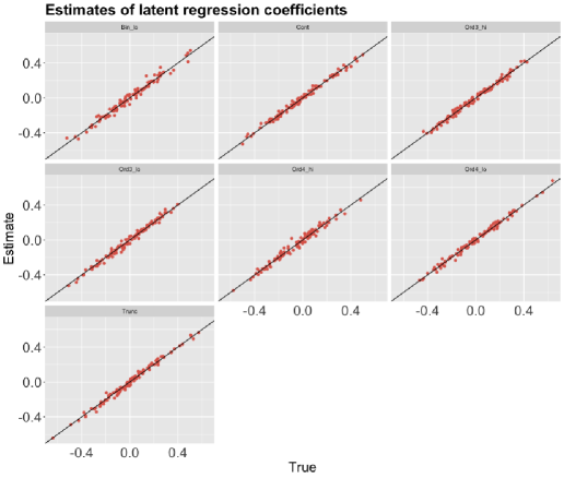
Figure 3: The estimates of latent regression coefficients over different simulation scenarios. The black line denotes $y=x$ line

For regression modeling, we treat $X_{1}$ (the binary variable with high entropy) as our outcome. We use methods described in Section 2.1 to estimate the latent correlation matrix and regression coefficients for each instance of the simulated data. We also calculate the asymptotic confidence intervals of our estimates from Theorem 3. Finally, for every instance of a simulated correlation matrix, we perform $500$ replicates of our experiment to get an empirical distribution of our estimated parameters. We calculate coverage of these $500$ estimates against the asymptotic confidence intervals to gauge the accuracy of the asymptotic intervals.

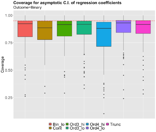
Figure 4: The coverage of $95\%$ asymptotic confidence interval for SGCRM regression coefficients. The red dotted line corresponds to the $0.95$ coverage.

Table 3: Mixed GLNPN variables

Variable number	Variable type	Cutpoint(s)
$X_{1}$	Binary (high entropy)	$0.3$
$X_{2}$	Continuous	Not applicable
$X_{3}$	Binary (low entropy)	$1$
$X_{4}$	Ordinal ($3$ categories and high entropy)	$(-0.1,0.6)$
$X_{5}$	Ordinal ($3$ categories and low entropy)	$(-1,1)$
$X_{6}$	Ordinal ($4$ categories and high entropy)	$(-0.7,0.1,0.6)$
$X_{7}$	Ordinal ($4$ categories and low entropy)	$(-0.3,0.1,0.2)$
$X_{8}$	Truncated	0

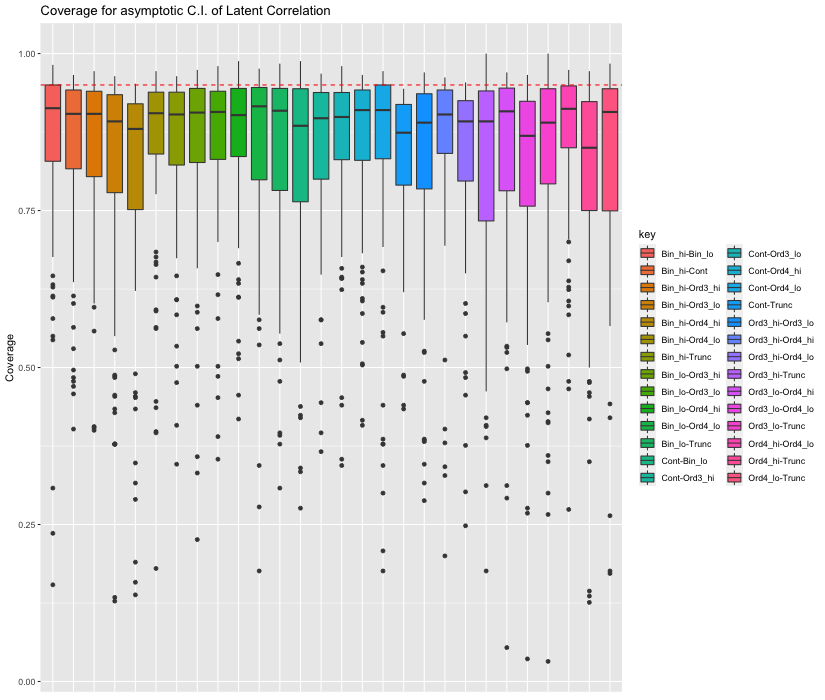
Figure S1: The coverage of the $95\%$ asymptotic confidence interval for latent correlations. The red dotted line denotes $0.95$ line

Figure 3 shows the estimates of latent regression coefficients against the true values. We observe that across different combinations, the estimated and true parameters are very well aligned along the diagonal line. We also report the coverage of our proposed asymptotic confidence interval for regression coefficients (Fig. S1). The median coverage (across $100$ seeds) of SGCRM regression coefficients is slightly below the expected $95\%$ line. This undercoverage is somewhat expected as we do not consider the estimated cutoffs’ uncertainty in calculating the asymptotic variances. Accounting for additional uncertainty from the use of plug-in cutoff estimators can be an interesting topic of future development of this framework.

6 Application of SGCRM in NHANES 2003-2006

In this section, we illustrate GLNPN and SGCRM in National Health and Nutrition Examination Survey (NHANES) $2003-2006$. We focus on the five variables discussed in Introduction: TAC, VPA, mortality, Health Status, and Mobility Problem. For the analysis, we excluded participants who (i) have missing mortality information or alive with follow-up less than 5 years, (ii) are younger than 50 years old or aged 85 and older, (iii) have missing any of the above-mentioned variables of interest, (iv) have died due to accident, and (v) had fewer than 3 valid accelerometry days (a valid day is defined as a day with at least 10 hours of wear time) (Leroux et al., 2019). The final analytical sample consisted of $3069$ subjects with $313$ deaths within $5$ years.

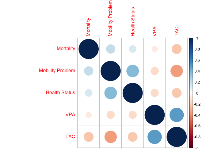
(a) Pearson correlation matrix

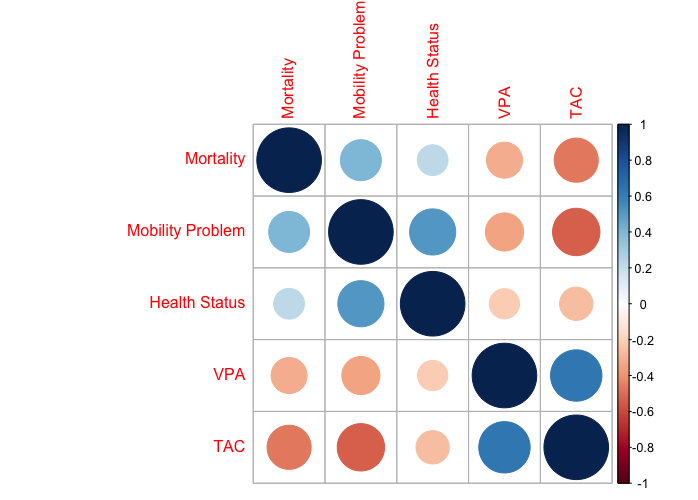
(b) GLNPN latent correlation matrix

Figure 5: The estimated $5\times 5$ correlation matrices of our variables from NHANES $2003-04$ and $2005-06$

Figure 5 compares estimated Pearson and latent correlation matrices (numerical values are given in Tables S1 and S2). We observe that the latent correlation matrix detects stronger correlation between variables compared to naively interpreting Pearson correlations for mixed types variables. For example, the correlation between Mortality and Mobility Problem increases from $0.2$ to $0.39$, the correlation between Mortality and VPA increases from $-0.08$ to $-0.30$.

Table 4: Comparison of simple linear model and SGCRM results for continuous outcome

$TAC\sim MobilityProblem+HealthStatus$
	Simple linear regression		SGCRM
	Covariate	Coefficients	Covariate	Coefficients
1	Mobility Problem (1)	-0.342 (-0.378, -0.306)	Mobility Problem	-0.543 (-0.594, -0.492)
2	Health Status (2)	-0.073 (-0.134, -0.013)	Health Status	0.011 (-0.036, 0.059)
3	Health Status (3)	-0.152 (-0.211, -0.094)		NA
4	Health Status (4)	-0.153 (-0.217, -0.09)		NA
5	Health Status (5)	-0.181 (-0.271, -0.09)		NA

Table 5: Comparison of truncated Gaussian regression and SGCRM results for truncated outcome

$VPA\sim MobilityProblem+HealthStatus$
	Truncated Gaussian regression		SGCRM
	Covariate	Coefficients	Covariate	Coefficients
1	Mobility Problem (1)	-629.875 (-753.338, -506.412)	Mobility Problem	-0.32 (-0.376, -0.265)
2	Health Status (2)	-63.201 (-88.362, -38.041)	Health Status	-0.055 (-0.108, -0.004)
3	Health Status (3)	-194.491 (-239.269, -149.714)		NA
4	Health Status (4)	-195.522 (-248.435, -142.608)		NA
5	Health Status (5)	-285.281 (-403.648, -166.914)		NA

Table 6: Comparison of probit ordinal regression and SGCRM results for ordinal outcome

$HealthStatus\sim MobilityProblem+VPA$
	Probit ordinal regression		SGCRM
	Covariate	Coefficients	Covariate	Coefficients
1	Mobility Problem (1)	0.874 (0.79, 0.959)	Mobility Problem	0.494 (0.45, 0.537)
2	I(VPA == 0)	0.12 (0.04, 0.199)		NA
3	VPA	-0.017 (-0.024, -0.011)	VPA	-0.047 (-0.091, -0.003)

Table 7: Comparison of probit regression and SGCRM results for binary outcome

$Mortality\sim MobilityProblem+HealthStatus+TAC$
	Probit regression		SGCRM
	Covariate	Coefficients	Covariate	Coefficients
1	Mobility Problem (1)	0.335 (0.192, 0.478)	Mobility Problem	0.195 (0.097, 0.297)
2	Health Status (2)	0.086 (-0.212, 0.402)	Health Status	0.033 (-0.042, 0.103)
3	Health Status (3)	0.244 (-0.038, 0.547)		NA
4	Health Status (4)	0.195 (-0.102, 0.511)		NA
5	Health Status (5)	0.455 (0.094, 0.826)		NA
6	TAC	$-3.952\times 10^{-6}(-4.752\times 10^{-6},-3.174*10^{-6})$	TAC	-0.352 (-0.427, -0.272)

After estimation of the GLNPN latent correlation matrix, we next fit four mutually consistent conditional SGCRM models by treating one of the mixed types variables as an outcome and some of the others as predictors. Specifically, we will consider one outcome for each type: TAC (continuous), VPA (truncated), Health Status (ordinal), and Mortality (binary). We compare the results from SGCRM models and their traditional counterparts including simple linear regression, truncated regression, ordinal probit and probit regressions in Tables 4, 5, 6, 7, respectively. Regression estimates are reported with $95\%$ confidence intervals. Our key focus is on comparing the direction and significance of conditional associations captured by SGCRM vs traditional models.

We start with a continuous outcome, TAC shown in Table 4. We observe that Mobility Problem has a significant negative effect on TAC in both SGCRM ($-0.543,CI:(-0.594,-0.492)$) and the linear model ($-0.342CI:(-0.378,-0.306)$). Furthermore, different levels of Health Status have a significant negative effect on TAC in the simple linear model, but not in SGCRM. SGCRM represents ordinal categories of Health Status via corresponding GLNPN latent variable and we do not observe a significant association with TAC in SGCRM model. This is one obvious disadvantage of our approach for ordinal variables. If the effect is not present across all levels, collapsing all levels may potentially loose partial significance, as we observe in this example. We will discuss this disadvantage more in Discussion.

Next, we treat truncated variable VPA as the outcome in SGCRM and compare SGCRM model vs Gaussian truncated regression model. The results are shown in Table 5. The direction and the significance of associations estimated by SGCRM are in agreement with those estimated by truncated regression. However, regression coefficients from truncated Gaussian regression model are not scaled and, hence, their magnitude cannot be compared. In contrast, SGCRM coefficients are normalized and can be compared across covariates. For example, we observe that the estimated effect of mobility problem is much higher that that of health status: $-0.32,CI:(-0.376,-0.265)$ vs $-0.055,CI:(-0.108,-0.004$).

Next, we model Health Status as an ordinal outcome with Mobility Problem and VPA as two covariates and compare SGCRM and probit ordinal model. Because, VPA is a truncated variable, we represent VPA via two components in the traditional model: (i) an indicator variable of VPA being equal to $0$, and (ii) the VPA value itself. Note that representation is not needed in SGCRM. The results are shown in Table 6. VPA is negatively associated with a higher value (worse) Health Status both in probit ordinal model with the regression coefficient of $-0.017,CI:(-0.024,-0.011)$ and in SGCRM model with the regression coefficient of $-0.047,CI:(-0.091,-0.003)$. Mobility problem is significant and is positively associated with a higher value (worse) Health Status in both models. Again, SGCRM allows to compare the magnitude of estimated effects of Mobility Problem and VPA with a much higher effect of the former.

Finally, we look at the 5-year mortality as a binary outcome with mobility problem, Health Status, and TAC as covariates and compare SGCRM and probit regression. The results are shown in Table 7. We see that the highest (worst) Health Status level is significant in probit regression, but when the ordinal categories of Health Status are represented via corresponding GLNPN latent variable we do not observe significant association with mortality in SGCRM model. Again, as we discussed above this is a limitation of SGCRM. We again get interpretable regression coefficients and we see that the effect of TAC is almost twice higher than of mobility problem.

It is important to note that all four SGCRM models are mutually consistent in contrast to the set of four traditional regressions: simple linear, truncated, probit ordinal, and probit.

We also calculate predictions of latent variables using methods described in Section 4.1. Figure 6 shows the distribution of the predicted latent variables for the five variables. The figure also shows the interrelation between those variables on the off-diagonal blocks of the scatterplot matrix. We see that the distribution of predicted latent variables approximates the assumed latent normal distribution, but with multiple modes originated from the discontinuities of the distributions of observed variables. It is interesting to note that scatterplots of predicted latent variables for mortality vs. mobility problem, mortality vs TAC, and TAC vs mobility problem reveal linear patterns (with some discontinuities around the cutoffs). This particular observation would be harder, if possible, to make by visually exploring scatterplots of observed counterparts.

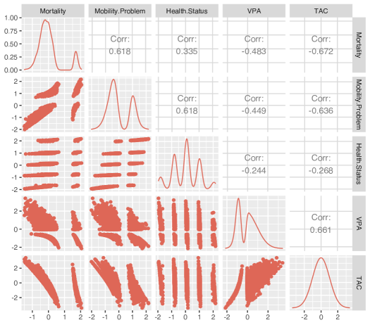
Figure 6: Predictions of latent variables in NHANES

7 Discussion

The main contribution of this paper is a joint modeling approach for mixed data types that builds on Semiparametric Gaussian Copula. SGCRM performs a linear regression on the latent SGC space and provides mutually consistent conditional regression models for continuous, truncated, ordinal, and binary outcomes. The approach is likelihood-free, scale-free, and more computationally efficient than likelihood-based joint copula models. SGCRM automatically normalizes the scale of all latent variables that results in standardized and cross-comparable regression coefficients. SGCRM provides $R^{2}$ analogs for all four types of outcomes. Finally, the approach allows to perform missing data imputation and latent variable prediction.

In NHANES, we focused only on five variables to carefully illustrate the approach and interpretability of the results. In terms of computational complexity, the approach only needs to calculate $O(p^{2})$ correlation parameters and the calculation of Kendall’s Tau takes only $O(nlogn)$ FLOPs for each correlation pair. Hence, with the quadratic complexity in $p$ the approach scales very well in $p$. Moreover, we proposed a novel computationally efficient way of calculating the asymptotic variance-covariance matrix of SGCRM regression estimates in $O(n^{2})$ FLOPs compared to the brute force approach of $O(n^{4})$.

In terms of limitations, SGCRM assumes a uniform magnitude and direction of the effect of latent variable and, thus, it is less flexible compared to modeling level-individual effects for ordinal variable. In the future work, more flexible GNLPN mechanisms using more than one latent variable can be considered to capture a possible non-uniform magnitude effect. SGCRM also loses interpretability of original scales of covariates, because SGCRM coefficients are only interpretable at a latent scale.

As future work, it would be important to develop quantile scale interpretation of SGCRM regression results. SGCRM can also be adapted to handle survival outcomes. Moreover, it would be interesting to adapt SGC to deal with functional and multi-level/longitudinal mixed data. As one of the methodological applications, we provided an algorithm for imputing missing observations and it would be very interesting to compare that approach with existing ones. Finally, predicted latent variables can be used for extending distance-based clustering and dimension reduction approaches to mixed data types.

Supplementary Materials

S1 Proofs

Proof of Theorem 1: Before we start the proof, let’s get familiar with some notations. Let us denote $\tilde{\Phi}_{2}((a,b),(c,d),\rho)$ as the probability of the rectangle $\{(u,v):a<u<c,b<v<d\}$ for a standard bivariate normal with correlation $\rho$. And, for $d>2$, $\tilde{\Phi}_{d}((a_{1},a_{2},\cdots,a_{d}),(b_{1},b_{2},\cdots,b_{d}),\rho)$ denotes the probability of the hyper-rectangle $\{(u_{1},u_{2},\cdots,u_{d}):a_{i}<u_{i}<b_{i},i=1,2,\cdots,d\}$.

Let $X_{j},X_{k}$ be ordinal with levels $\{0,1,\cdots,l_{j}-1\}$ and $\{0,1,\cdots,l_{k}-1\}$ respectively and $(L_{j},L_{k})$ is the corresponding latent standard bivariate normal with correlation $\rho$. Then for two independent observations $i,i^{\prime}$ -

$$P(X_{ij}>X_{i^{\prime}j},X_{ik}>X_{i^{\prime}k})$$

$$=\sum_{r=1}^{l_{j}-1}\sum_{s=1}^{l_{s}-1}[P(X_{ij}=r,X_{ik}=s)P(X_{i^{\prime}j}<r,X_{i^{\prime}k}<s)]$$

$$=\sum_{r=1}^{l_{j}-1}\sum_{s=1}^{l_{s}-1}[P(\Delta_{jr}\leq L_{ij}<\Delta_{j(r+1)},\Delta_{ks}\leq L_{ik}<\Delta_{(k+1)s})P(L_{i^{\prime}j}<\Delta_{jr},L_{i^{\prime}k}<\Delta_{ks})]$$

$$=\sum_{r=1}^{l_{j}-1}\sum_{s=1}^{l_{k}-1}[\tilde{\Phi}_{2}((\Delta_{jr},\Delta_{ks}),(\Delta_{j(r+1)},\Delta_{k(s+1)};\rho)\tilde{\Phi}_{2}((-\infty,-\infty),(\Delta_{jr},\Delta_{ks});\rho)]$$

Similarly,

$$P(X_{ij}>X_{i^{\prime}j},X_{ik}<X_{i^{\prime}k})$$

$$=\sum_{r=1}^{l_{j}-1}\sum_{s=1}^{l_{s}-1}[P(X_{ij}=r,X_{ik}=s-1)P(X_{i^{\prime}j}<r,X_{i^{\prime}k}>(s-1))]$$

$$=\sum_{r=1}^{l_{j}-1}\sum_{s=1}^{l_{s}-1}[P(\Delta_{jr}\leq L_{ij}<\Delta_{j(r+1)},\Delta_{(k-1)s}\leq L_{ik}<\Delta_{ks})P(L_{i^{\prime}j}<\Delta_{jr},L_{i^{\prime}k}>\Delta_{ks})]$$

$$=\sum_{r=1}^{l_{j}-1}\sum_{s=1}^{l_{s}-1}[P(\Delta_{jr}\leq L_{ij}<\Delta_{j(r+1)},\Delta_{(k-1)s}\leq L_{ik}<\Delta_{ks})P(L_{i^{\prime}j}<\Delta_{jr},-L_{i^{\prime}k}<-\Delta_{ks})]$$

$$=\sum_{r=1}^{l_{j}-1}\sum_{s=1}^{l_{k}-1}[\tilde{\Phi}_{2}((\Delta_{jr},\Delta_{k(s-1)}),(\Delta_{j(r+1)},\Delta_{ks};\rho)\tilde{\Phi}_{2}((-\infty,-\infty),(\Delta_{jr},-\Delta_{ks});-\rho)]$$

By symmetry, the population Kendall’s Tau, $\tau_{jk}$ for $X_{j},X_{k}$ can be written as follows -

$$\tau_{jk}= 2(P(X_{ij}>X_{i^{\prime}j},X_{ik}>X_{i^{\prime}k})-P(X_{ij}>X_{i^{\prime}j},X_{ik}<X_{i^{\prime}k}))$$

$$= 2(\sum_{r=1}^{l_{j}-1}\sum_{s=1}^{l_{k}-1}[\tilde{\Phi}_{2}((\Delta_{jr},\Delta_{ks}),(\Delta_{j(r+1)},\Delta_{k(s+1)};\rho)\tilde{\Phi}_{2}((-\infty,-\infty),(\Delta_{jr},\Delta_{ks});\rho)$$

$$-\tilde{\Phi}_{2}((\Delta_{jr},\Delta_{k(s-1)}),(\Delta_{j(r+1)},\Delta_{ks};\rho)\tilde{\Phi}_{2}((-\infty,-\infty),(\Delta_{jr},-\Delta_{ks});-\rho)])$$

$$= 2\sum_{r=1}^{l_{j}-1}\sum_{s=1}^{l_{k}-1}[\{\Phi_{2}(\Delta_{jr},\Delta_{ks};\rho)+\Phi_{2}(\Delta_{j(r+1)},\Delta_{k(s+1)};\rho)-$$

$$\Phi_{2}(\Delta_{jr},\Delta_{k(s+1)};\rho)-\Phi_{2}(\Delta_{j(r+1)},\Delta_{ks};\rho)\}\Phi_{2}(\Delta_{jr},\Delta_{ks};\rho)-$$

$$\{\Phi_{2}(\Delta_{jr},\Delta_{k(s-1)};\rho)+\Phi_{2}(\Delta_{j(r+1)},\Delta_{ks};\rho)-$$

$$\Phi_{2}(\Delta_{jr},\Delta_{ks};\rho)-\Phi_{2}(\Delta_{j(r+1)},\Delta_{k(s-1)};\rho)\}(\Phi(\Delta_{jr})-\Phi_{2}(\Delta_{jr},\Delta_{ks};\rho))]$$

$$= 2\sum_{r=1}^{l_{j}-1}\sum_{s=1}^{l_{k}-1}[\Phi_{2}(\Delta_{jr},\Delta_{ks};\rho)\{\Phi_{2}(\Delta_{jr},\Delta_{ks};\rho)+\Phi_{2}(\Delta_{j(r+1)},\Delta_{k(s+1)};\rho)-$$

$$\Phi_{2}(\Delta_{jr},\Delta_{k(s+1)};\rho)-\Phi_{2}(\Delta_{j(r+1)},\Delta_{ks};\rho)$$

$$+\Phi_{2}(\Delta_{jr},\Delta_{k(s-1)};\rho)+\Phi_{2}(\Delta_{j(r+1)},\Delta_{ks};\rho)-\Phi_{2}(\Delta_{jr},\Delta_{ks};\rho)-\Phi_{2}(\Delta_{j(r+1)},\Delta_{k(s-1)};\rho)\}]-$$

$$2\sum_{r=1}^{l_{j}-1}\Phi({\Delta_{jr}})\sum_{s=1}^{l_{k}-1}[\Phi_{2}(\Delta_{jr},\Delta_{k(s-1)};\rho)+\Phi_{2}(\Delta_{j(r+1)},\Delta_{ks};\rho)-$$

$$\Phi_{2}(\Delta_{jr},\Delta_{ks};\rho)-\Phi_{2}(\Delta_{j(r+1)},\Delta_{k(s-1)};\rho)]$$

$$= 2\sum_{r=1}^{l_{j}-1}\sum_{s=1}^{l_{k}-1}[\Phi_{2}(\Delta_{jr},\Delta_{ks};\rho)\{\Phi_{2}(\Delta_{j(r+1)},\Delta_{k(s+1)};\rho)-\Phi_{2}(\Delta_{jr},\Delta_{k(s+1)};\rho)$$

$$+\Phi_{2}(\Delta_{jr},\Delta_{k(s-1)};\rho)-\Phi_{2}(\Delta_{j(r+1)},\Delta_{k(s-1)};\rho)\}]-$$

$$2\sum_{r=1}^{l_{j}-1}\Phi({\Delta_{jr}})[-\Phi_{2}(\Delta_{jr},\Delta_{k(l_{k}-1)};\rho)+\Phi_{2}(\Delta_{j(r+1)},\Delta_{k(l_{k}-1)};\rho)]$$

$$= 2\sum_{r=1}^{l_{j}-1}\sum_{s=1}^{l_{k}-1}[\Phi_{2}(\Delta_{jr},\Delta_{ks};\rho)\{\Phi_{2}(\Delta_{j(r+1)},\Delta_{k(s+1)};\rho)-\Phi_{2}(\Delta_{j(r+1)},\Delta_{k(s-1)};\rho)\}]+$$

$$2\sum_{r=1}^{l_{j}-1}[\sum_{s=1}^{l_{k}-1}\Phi_{2}(\Delta_{jr},\Delta_{ks};\rho)\Phi_{2}(\Delta_{jr},\Delta_{k(s-1)};\rho)-\Phi_{2}(\Delta_{jr},\Delta_{ks};\rho)\Phi_{2}(\Delta_{jr},\Delta_{k(s+1)};\rho)]-$$

$$2\sum_{r=1}^{l_{j}-1}\Phi({\Delta_{jr}})[-\Phi_{2}(\Delta_{jr},\Delta_{k(l_{k}-1)};\rho)+\Phi_{2}(\Delta_{j(r+1)},\Delta_{k(l_{k}-1)};\rho)]$$

$$= 2\sum_{r=1}^{l_{j}-1}\sum_{s=1}^{l_{k}-1}[\Phi_{2}(\Delta_{jr},\Delta_{ks};\rho)\{\Phi_{2}(\Delta_{j(r+1)},\Delta_{k(s+1)};\rho)-\Phi_{2}(\Delta_{j(r+1)},\Delta_{k(s-1)};\rho)\}]+$$

$$2\sum_{r=1}^{l_{j}-1}[\Phi_{2}(\Delta_{jr},\Delta_{k1};\rho)\Phi_{2}(\Delta_{jr},\Delta_{k0};\rho)-\Phi_{2}(\Delta_{jr},\Delta_{k(l_{k}-1)};\rho)\Phi_{2}(\Delta_{jr},\Delta_{k(l_{k})};\rho)]-$$

$$2\sum_{r=1}^{l_{j}-1}\Phi({\Delta_{jr}})[-\Phi_{2}(\Delta_{jr},\Delta_{k(l_{k}-1)};\rho)+\Phi_{2}(\Delta_{j(r+1)},\Delta_{k(l_{k}-1)};\rho)]$$

$$= 2\sum_{r=1}^{l_{j}-1}\sum_{s=1}^{l_{k}-1}[\Phi_{2}(\Delta_{jr},\Delta_{ks};\rho)\{\Phi_{2}(\Delta_{j(r+1)},\Delta_{k(s+1)};\rho)-\Phi_{2}(\Delta_{j(r+1)},\Delta_{k(s-1)};\rho)\}]+$$

$$2\sum_{r=1}^{l_{j}-1}[-\Phi_{2}(\Delta_{jr},\Delta_{k(l_{k}-1)};\rho)\Phi(\Delta_{jr})]-$$

$$2\sum_{r=1}^{l_{j}-1}\Phi({\Delta_{jr}})[-\Phi_{2}(\Delta_{jr},\Delta_{k(l_{k}-1)};\rho)+\Phi_{2}(\Delta_{j(r+1)},\Delta_{k(l_{k}-1)};\rho)]$$

$$= 2\sum_{r=1}^{l_{j}-1}\sum_{s=1}^{l_{k}-1}[\Phi_{2}(\Delta_{jr},\Delta_{ks};\rho)\{\Phi_{2}(\Delta_{j(r+1)},\Delta_{k(s+1)};\rho)-\Phi_{2}(\Delta_{j(r+1)},\Delta_{k(s-1)};\rho)\}]-$$

$$2\sum_{r=1}^{l_{j}-1}\Phi({\Delta_{jr}})\Phi_{2}(\Delta_{j(r+1)},\Delta_{k(l_{k}-1)};\rho)$$

The third equality follows from the fact that - $\tilde{\Phi}_{2}((a,b),(c,d);\rho)={\Phi}_{2}((a,b);\rho)+{\Phi}_{2}((c,d);\rho)-{\Phi}_{2}((a,d);\rho)-{\Phi}_{2}((c,b);\rho)$. The seventh equality comes from the following result - for a sequence $\{a_{s}\}_{s=0}^{n},\sum_{s=1}^{n-1}(a_{s}a_{s-1}-a_{s}a_{s+1})=(a_{1}a_{0}-a_{n-1}a_{n})$.

Now, reducing the above calculations for $l_{k}=2$, will yield the bridging function between a general ordinal and binary pairs.

Now, suppose we have a truncated variable $X_{m}$ with cutoff $\Delta_{m}$ and corresponding latent normal variable $L_{m}$. For consistency in bridging function expressions, we slightly abuse notations to denote $\rho$ as the latent correlation between the truncated and the ordinal variable. Then similar to the ordinal-ordinal case, the calculations will look like -

$$P(X_{ij}>X_{i^{\prime}j},X_{im}>X_{i^{\prime}m})$$

$$=\sum_{r=1}^{l_{j}-1}[P(X_{ij}=r,X_{im}>0)P(X_{i^{\prime}j}<r,X_{i^{\prime}m}=0)$$

$$+P(X_{ij}=r,X_{i^{\prime}j}<r,X_{i^{\prime}m}>0,X_{im}-X_{i^{\prime}m}>0)]$$

$$=\sum_{r=1}^{l_{j}-1}[P(\Delta_{jr}\leq L_{ij}<\Delta_{j(r+1)},L_{im}>\Delta_{m})P(L_{i^{\prime}j}<\Delta_{jr},L_{i^{\prime}m}\leq\Delta_{m})$$

$$+P(\Delta_{jr}\leq L_{ij}<\Delta_{j(r+1)},L_{i^{\prime}j}<\Delta_{jr},L_{i^{\prime}m}>\Delta_{m},,\frac{L_{im}-L_{i^{\prime}m}}{2}>0)]$$

$$=\sum_{r=1}^{l_{j}-1}[P(\Delta_{jr}\leq L_{ij}<\Delta_{j(r+1)},-L_{im}<-\Delta_{m})P(L_{i^{\prime}j}<\Delta_{jr},L_{i^{\prime}m}\leq\Delta_{m})$$

$$+P(-\Delta_{j(r+1)}\leq-L_{ij}<-\Delta_{jr},L_{i^{\prime}j}<\Delta_{jr},L_{i^{\prime}m}>\Delta_{m},,\frac{L_{i^{\prime}m}-L_{im}}{\sqrt{2}}<0)]$$

$$=\sum_{r=1}^{l_{j}-1}[\tilde{\Phi}_{2}((\Delta_{jr},-\infty),(\Delta_{j(r+1)},-\Delta_{m});-\rho)\tilde{\Phi}_{2}((-\infty,-\infty),(\Delta_{jr},\Delta_{m});\rho)+$$

$$\tilde{\Phi}_{4}((-\Delta_{j(r+1)},-\infty,\Delta_{m},-\infty),(-\Delta_{jr},\Delta_{jr},\infty,0);S_{5a}(\rho))]$$

$$=\sum_{r=1}^{l_{j}-1}[\tilde{\Phi}_{2}((\Delta_{jr},-\infty),(\Delta_{j(r+1)},-\Delta_{m});-\rho)\tilde{\Phi}_{2}((-\infty,-\infty),(\Delta_{jr},\Delta_{m});\rho)$$

$$+\tilde{\Phi}_{3}((-\Delta_{j(r+1)},-\infty,-\infty),(-\Delta_{jr},\Delta_{jr},0);\begin{pmatrix}1&0&\frac{\rho}{\sqrt{2}}\\ 0&1&\frac{\rho}{\sqrt{2}}\\ \frac{\rho}{\sqrt{2}}&\frac{\rho}{\sqrt{2}}&1\end{pmatrix})-$$

$$\tilde{\Phi}_{4}((-\Delta_{j(r+1)},-\infty,-\infty,-\infty),(-\Delta_{jr},\Delta_{jr},\Delta_{m},0);S_{5a}(\rho))]$$

$$=\sum_{r=1}^{l_{j}-1}[T_{1r}^{(1)}+T_{2r}^{(1)}-T_{3r}^{(1)}]$$ (S1)

$$P(X_{ij}<X_{i^{\prime}j},X_{im}>X_{i^{\prime}m})$$

$$=\sum_{r=1}^{l_{j}-1}[P(X_{ij}=(r-1),X_{im}>0)P(X_{i^{\prime}j}>(r-1),X_{i^{\prime}m}=0)$$

$$+P(X_{ij}=(r-1),X_{i^{\prime}j}>(r-1),X_{i^{\prime}m}>0,X_{im}-X_{i^{\prime}m}>0)]$$

$$=\sum_{r=1}^{l_{j}-1}[P(\Delta_{j(r-1)}\leq L_{ij}<\Delta_{jr},L_{im}>\Delta_{m})P(L_{i^{\prime}j}>\Delta_{jr},L_{i^{\prime}m}\leq\Delta_{m})$$

$$+P(\Delta_{j(r-1)}\leq L_{ij}<\Delta_{jr},L_{i^{\prime}j}>\Delta_{jr},L_{i^{\prime}m}>\Delta_{m},,\frac{L_{im}-L_{i^{\prime}m}}{\sqrt{2}}>0)]$$

$$=\sum_{r=1}^{l_{j}-1}[P(\Delta_{j(r-1)}\leq L_{ij}<\Delta_{jr},-L_{im}<-\Delta_{m})P(-L_{i^{\prime}j}<-\Delta_{jr},L_{i^{\prime}m}\leq\Delta_{m})$$

$$+P(-\Delta_{(jr}\leq-L_{ij}<-\Delta_{j(r-1)},L_{i^{\prime}j}>\Delta_{jr},L_{i^{\prime}m}>\Delta_{m},,\frac{L_{i^{\prime}m}-L_{im}}{\sqrt{2}}<0)]$$

$$=\sum_{r=1}^{l_{j}-1}[\tilde{\Phi}_{2}((\Delta_{j(r-1)},-\infty),(\Delta_{jr},-\Delta_{m});-\rho)\tilde{\Phi}_{2}((-\infty,-\infty),(-\Delta_{jr},\Delta_{m});-\rho)+$$

$$\tilde{\Phi}_{4}((-\Delta_{jr},\Delta_{jr},\Delta_{m},-\infty),(-\Delta_{j(r-1)},\infty,\infty,0);S_{5a}(\rho))]$$

$$=\sum_{r=1}^{l_{j}-1}[\tilde{\Phi}_{2}((\Delta_{j(r-1)},-\infty),(\Delta_{jr},-\Delta_{m});-\rho)\tilde{\Phi}_{2}((-\infty,-\infty),(-\Delta_{jr},\Delta_{m});-\rho)+$$

$$\tilde{\Phi}_{3}((-\Delta_{jr},\Delta_{m},-\infty),(-\Delta_{j(r-1)},\infty,0);S_{6b}(\rho))-\tilde{\Phi}_{4}((-\Delta_{jr},-\infty,\Delta_{m},-\infty),(-\Delta_{j(r-1)},\Delta_{jr},\infty,0);S_{5a}(\rho))]$$

$$=\sum_{r=1}^{l_{j}-1}[\tilde{\Phi}_{2}((\Delta_{j(r-1)},-\infty),(\Delta_{jr},-\Delta_{m});-\rho)\tilde{\Phi}_{2}((-\infty,-\infty),(-\Delta_{jr},\Delta_{m});-\rho)+$$

$$\tilde{\Phi}_{2}((-\Delta_{jr},-\infty),(-\Delta_{j(r-1)},0);\frac{\rho}{\sqrt{2}})-\tilde{\Phi}_{3}((-\Delta_{jr},-\infty,-\infty),(-\Delta_{j(r-1)},\Delta_{m},0);S_{6b}(\rho))-$$

$$\tilde{\Phi}_{3}((-\Delta_{jr},-\infty,-\infty),(-\Delta_{j(r-1)},\Delta_{jr},0);\begin{pmatrix}1&0&\frac{\rho}{\sqrt{2}}\\ 0&1&\frac{\rho}{\sqrt{2}}\\ \frac{\rho}{\sqrt{2}}&\frac{\rho}{\sqrt{2}}&1\end{pmatrix})+$$

$$\tilde{\Phi}_{4}((-\Delta_{jr},-\infty,-\infty,-\infty),(-\Delta_{j(r-1)},\Delta_{jr},\Delta_{m},0);S_{5a}(\rho))]$$

$$=\sum_{r=1}^{l_{j}-1}[T_{1r}^{(2)}+T_{2r}^{(2)}-T_{3r}^{(2)}-T_{4r}^{(2)}+T_{5r}^{(2)}]$$ (S2)

where, $S_{5a}(\rho)=\textrm{cov}(-L_{ij},L_{i^{\prime}j},L_{i^{\prime}m},\frac{L_{i^{\prime}m}-L_{im}}{\sqrt{2}})=\begin{pmatrix}1&0&0&\frac{\rho}{\sqrt{2}}\\ 0&1&\rho&\frac{\rho}{\sqrt{2}}\\ 0&\rho&1&\frac{1}{\sqrt{2}}\\ \frac{\rho}{\sqrt{2}}&\frac{\rho}{\sqrt{2}}&\frac{1}{\sqrt{2}}&1\end{pmatrix}$ and
$S_{5b}(\rho)=cov(L_{ij},-L_{i^{\prime}j},-L_{i^{\prime}m},\frac{L_{i^{\prime}m}-L_{im}}{\sqrt{2}})=\begin{pmatrix}1&0&0&-\frac{\rho}{\sqrt{2}}\\ 0&1&\rho&-\frac{\rho}{\sqrt{2}}\\ 0&\rho&1&-\frac{1}{\sqrt{2}}\\ -\frac{\rho}{\sqrt{2}}&-\frac{\rho}{\sqrt{2}}&-\frac{1}{\sqrt{2}}&1\end{pmatrix}$.

$$\sum_{r=1}^{l_{j}-1}[T_{2r}^{(1)}+T_{4r}^{(2)}]$$

$$=\sum_{r=1}^{l_{j}-1}[\Phi_{3}((-\Delta_{jr},\Delta_{jr},0);\begin{pmatrix}1&0&\frac{\rho}{\sqrt{2}}\\ 0&1&\frac{\rho}{\sqrt{2}}\\ \frac{\rho}{\sqrt{2}}&\frac{\rho}{\sqrt{2}}&1\end{pmatrix})-\Phi_{3}((-\Delta_{j(r+1)},\Delta_{jr},0);\begin{pmatrix}1&0&\frac{\rho}{\sqrt{2}}\\ 0&1&\frac{\rho}{\sqrt{2}}\\ \frac{\rho}{\sqrt{2}}&\frac{\rho}{\sqrt{2}}&1\end{pmatrix})+$$

$$\Phi_{3}((-\Delta_{j(r-1)},\Delta_{jr},0);\begin{pmatrix}1&0&\frac{\rho}{\sqrt{2}}\\ 0&1&\frac{\rho}{\sqrt{2}}\\ \frac{\rho}{\sqrt{2}}&\frac{\rho}{\sqrt{2}}&1\end{pmatrix})-\Phi_{3}((-\Delta_{jr},\Delta_{jr},0);\begin{pmatrix}1&0&\frac{\rho}{\sqrt{2}}\\ 0&1&\frac{\rho}{\sqrt{2}}\\ \frac{\rho}{\sqrt{2}}&\frac{\rho}{\sqrt{2}}&1\end{pmatrix})$$

$$=\sum_{r=1}^{l_{j}-1}[\Phi_{3}((-\Delta_{j(r-1)},\Delta_{jr},0);\begin{pmatrix}1&0&\frac{\rho}{\sqrt{2}}\\ 0&1&\frac{\rho}{\sqrt{2}}\\ \frac{\rho}{\sqrt{2}}&\frac{\rho}{\sqrt{2}}&1\end{pmatrix})-\Phi_{3}((-\Delta_{j(r+1)},\Delta_{jr},0);\begin{pmatrix}1&0&\frac{\rho}{\sqrt{2}}\\ 0&1&\frac{\rho}{\sqrt{2}}\\ \frac{\rho}{\sqrt{2}}&\frac{\rho}{\sqrt{2}}&1\end{pmatrix})]$$

$$=\sum_{r=1}^{l_{j}-1}[\Phi_{2}(-\Delta_{j(r-1)},\Delta_{jr};0)-\Phi_{3}((-\Delta_{j(r-1)},\Delta_{jr},0);\begin{pmatrix}1&0&-\frac{\rho}{\sqrt{2}}\\ 0&1&-\frac{\rho}{\sqrt{2}}\\ -\frac{\rho}{\sqrt{2}}&-\frac{\rho}{\sqrt{2}}&1\end{pmatrix})-$$

$$\Phi_{2}(-\Delta_{j(r-1)},\Delta_{jr};0)+\Phi_{3}((-\Delta_{j(r+1)},\Delta_{jr},0);\begin{pmatrix}1&0&-\frac{\rho}{\sqrt{2}}\\ 0&1&-\frac{\rho}{\sqrt{2}}\\ -\frac{\rho}{\sqrt{2}}&-\frac{\rho}{\sqrt{2}}&1\end{pmatrix})]$$

$$=\sum_{r=1}^{l_{j}-1}[\Phi(-\Delta_{j(r-1)})\Phi(\Delta_{jr})-\Phi(-\Delta_{j(r+1)})\Phi(\Delta_{jr})]-$$

$$\sum_{r=1}^{l_{j}-1}[\Phi_{3}((-\Delta_{j(r-1)},\Delta_{jr},0);\begin{pmatrix}1&0&-\frac{\rho}{\sqrt{2}}\\ 0&1&-\frac{\rho}{\sqrt{2}}\\ -\frac{\rho}{\sqrt{2}}&-\frac{\rho}{\sqrt{2}}&1\end{pmatrix})-$$

$$\Phi_{3}((-\Delta_{j(r+1)},\Delta_{jr},0);\begin{pmatrix}1&0&-\frac{\rho}{\sqrt{2}}\\ 0&1&-\frac{\rho}{\sqrt{2}}\\ -\frac{\rho}{\sqrt{2}}&-\frac{\rho}{\sqrt{2}}&1\end{pmatrix})]$$

$$=\Phi(\Delta_{j(l_{j}-1)})-\sum_{r=1}^{l_{j}-1}[\Phi_{3}((-\Delta_{j(r-1)},\Delta_{jr},0);\begin{pmatrix}1&0&-\frac{\rho}{\sqrt{2}}\\ 0&1&-\frac{\rho}{\sqrt{2}}\\ -\frac{\rho}{\sqrt{2}}&-\frac{\rho}{\sqrt{2}}&1\end{pmatrix})-$$

$$\Phi_{3}((-\Delta_{j(r+1)},\Delta_{jr},0);\begin{pmatrix}1&0&-\frac{\rho}{\sqrt{2}}\\ 0&1&-\frac{\rho}{\sqrt{2}}\\ -\frac{\rho}{\sqrt{2}}&-\frac{\rho}{\sqrt{2}}&1\end{pmatrix})]$$ (S3)

$$\sum_{r=1}^{l_{j}-1}[T_{3r}^{(1)}+T_{5r}^{(2)}]$$

$$=\sum_{r=1}^{l_{j}-1}[\Phi_{4}((-\Delta_{jr},\Delta_{jr},\Delta_{m},0);S_{5a}(\rho))-\Phi_{4}((-\Delta_{j(r+1)},\Delta_{jr},\Delta_{m},0);S_{5a}(\rho))+$$

$$-\Phi_{4}((-\Delta_{jr},\Delta_{jr},\Delta_{m},0);S_{5a}(\rho))+\Phi_{4}((-\Delta_{j(r-1)},\Delta_{jr},\Delta_{m},0);S_{5a}(\rho))]$$

$$=\sum_{r=1}^{l_{j}-1}[\Phi_{4}((-\Delta_{j(r-1)},\Delta_{jr},\Delta_{m},0);S_{5a}(\rho))-\Phi_{4}((-\Delta_{j(r+1)},\Delta_{jr},\Delta_{m},0);S_{5a}(\rho))]$$

$$\sum_{r=1}^{l_{j}-1}[T_{2r}^{(2)}-T_{3r}^{(2)}]$$

$$=\sum_{r=1}^{l_{j}-1}[\tilde{\Phi}_{2}((-\Delta_{jr},-\infty),(-\Delta_{j(r-1)},0);\frac{\rho}{\sqrt{2}})]-$$

$$\sum_{r=1}^{l_{j}-1}[\tilde{\Phi}_{3}((-\Delta_{jr},-\infty,-\infty),(-\Delta_{j(r-1)},\Delta_{m},0);\begin{pmatrix}1&0&\frac{\rho}{\sqrt{2}}\\ 0&1&\frac{1}{\sqrt{2}}\\ \frac{\rho}{\sqrt{2}}&\frac{1}{\sqrt{2}}&1\end{pmatrix}]$$

$$=\sum_{r=1}^{l_{j}-1}[\Phi_{2}((-\Delta_{j(r-1)},0);\frac{\rho}{\sqrt{2}})-\Phi_{2}((-\Delta_{jr},0);\frac{\rho}{\sqrt{2}})]-$$

$$\sum_{r=1}^{l_{j}-1}[\Phi_{3}((-\Delta_{j(r-1)},\Delta_{m},0);\begin{pmatrix}1&0&\frac{\rho}{\sqrt{2}}\\ 0&1&\frac{1}{\sqrt{2}}\\ \frac{\rho}{\sqrt{2}}&\frac{1}{\sqrt{2}}&1\end{pmatrix})-\Phi_{3}((-\Delta_{jr},\Delta_{m},0);\begin{pmatrix}1&0&\frac{\rho}{\sqrt{2}}\\ 0&1&\frac{1}{\sqrt{2}}\\ \frac{\rho}{\sqrt{2}}&\frac{1}{\sqrt{2}}&1\end{pmatrix})]$$

$$=\frac{1}{2}-\Phi_{2}(-\Delta_{j(l_{j}-1)},0;\frac{\rho}{\sqrt{2}})-(\Phi_{2}((\Delta_{m},0);\frac{1}{\sqrt{2}})-\Phi_{3}((-\Delta_{j(l_{j}-1)},\Delta_{m},0);\begin{pmatrix}1&0&\frac{\rho}{\sqrt{2}}\\ 0&1&\frac{1}{\sqrt{2}}\\ \frac{\rho}{\sqrt{2}}&\frac{1}{\sqrt{2}}&1\end{pmatrix}))$$

$$=\Phi_{2}(\Delta_{j(l_{j}-1)},0;-\frac{\rho}{\sqrt{2}})-\Phi_{3}((\Delta_{j(l_{j}-1)},\Delta_{m},0);\begin{pmatrix}1&0&\frac{-\rho}{\sqrt{2}}\\ 0&1&\frac{1}{\sqrt{2}}\\ \frac{-\rho}{\sqrt{2}}&\frac{1}{\sqrt{2}}&1\end{pmatrix}))$$

$$=\Phi_{3}((\Delta_{j(l_{j}-1)},-\Delta_{m},0);\begin{pmatrix}1&0&\frac{-\rho}{\sqrt{2}}\\ 0&1&\frac{-1}{\sqrt{2}}\\ \frac{-\rho}{\sqrt{2}}&\frac{-1}{\sqrt{2}}&1\end{pmatrix}))$$

$$\sum_{r=1}^{l_{j}-1}[T_{1r}^{(1)}-T_{1r}^{(2)}]$$

$$=\sum_{r=1}^{l_{j}-1}[\tilde{\Phi}_{2}((\Delta_{jr},-\infty),(\Delta_{j(r+1)},-\Delta_{m});-\rho)\tilde{\Phi}_{2}((-\infty,-\infty),(\Delta_{jr},\Delta_{m});\rho)-$$

$$\tilde{\Phi}_{2}((\Delta_{j(r-1)},-\infty),(\Delta_{jr},-\Delta_{m});-\rho)\tilde{\Phi}_{2}((-\infty,-\infty),(-\Delta_{jr},\Delta_{m});-\rho)]$$

$$=\sum_{r=1}^{l_{j}-1}[\Phi_{2}(\Delta_{jr},\Delta_{m};\rho)\{\Phi_{2}(\Delta_{jr},\Delta_{m};\rho)+\Phi(\Delta_{j(r+1)})-\Phi(\Delta_{jr})-\Phi_{2}(\Delta_{j(r+1)},\Delta_{m};\rho)\}-$$

$$(\Phi(\Delta_{m})-\Phi_{2}(\Delta_{jr},\Delta_{m};\rho))\{\Phi_{2}(\Delta_{j(r-1)},\Delta_{m};\rho)+\Phi(\Delta_{jr})-\Phi(\Delta_{j(r-1)})-\Phi_{2}(\Delta_{jr},\Delta_{m};\rho)\}]$$

$$=\sum_{r=1}^{l_{j}-1}[\Phi_{2}(\Delta_{jr},\Delta_{m};\rho)\{\Phi_{2}(\Delta_{jr},\Delta_{m};\rho)+\Phi(\Delta_{j(r+1)})-\Phi(\Delta_{jr})-$$

$$\Phi_{2}(\Delta_{j(r+1)},\Delta_{m};\rho)+\Phi_{2}(\Delta_{j(r-1)},\Delta_{m};\rho)+\Phi(\Delta_{jr})-\Phi(\Delta_{j(r-1)})-\Phi_{2}(\Delta_{jr},\Delta_{m};\rho)+\Phi(\Delta_{m})\}-$$

$$\Phi(\Delta_{m})\{\Phi_{2}(\Delta_{j(r-1)},\Delta_{m};\rho)+\Phi(\Delta_{jr})-\Phi(\Delta_{j(r-1)})\}]$$

$$=\sum_{r=1}^{l_{j}-1}[\Phi_{2}(\Delta_{jr},\Delta_{m};\rho)\{\Phi_{2}(\Delta_{jr},\Delta_{m};\rho)+\Phi(\Delta_{j(r+1)})-\Phi(\Delta_{jr})-\Phi_{2}(\Delta_{j(r+1)},\Delta_{m};\rho)\}-$$

$$(\Phi(\Delta_{m})-\Phi_{2}(\Delta_{jr},\Delta_{m};\rho))\{\Phi_{2}(\Delta_{j(r-1)},\Delta_{m};\rho)+\Phi(\Delta_{jr})-\Phi(\Delta_{j(r-1)})-\Phi_{2}(\Delta_{jr},\Delta_{m};\rho)\}]+$$

$$=\sum_{r=1}^{l_{j}-1}[\Phi_{2}(\Delta_{jr},\Delta_{m};\rho)\{\Phi(\Delta_{j(r+1)})-\Phi(\Delta_{j(r-1)})\}+$$

$$\{\Phi_{2}(\Delta_{jr},\Delta_{m};\rho)\Phi_{2}(\Delta_{j(r-1)},\Delta_{m};\rho)-\Phi_{2}(\Delta_{j(r+1)},\Delta_{m};\rho)\Phi_{2}(\Delta_{jr},\Delta_{m};\rho)\}]-$$

$$\Phi(\Delta_{m})[\sum_{r=1}^{l_{j}-1}\{\Phi_{2}(\Delta_{j(r-1)},\Delta_{m};\rho)-\Phi_{2}(\Delta_{jr},\Delta_{m};\rho)\}+\sum_{r=1}^{l_{j}-1}\{\Phi(\Delta_{jr})-\Phi(\Delta_{j(r-1)})\}]+$$

$$=\sum_{r=1}^{l_{j}-1}[\Phi_{2}(\Delta_{jr},\Delta_{m};\rho)\{\Phi(\Delta_{j(r+1)})-\Phi(\Delta_{j(r-1)})\}]$$

$$-\Phi(\Delta_{m})\Phi_{2}(\Delta_{j(l_{j}-1)},\Delta_{m};\rho)+2\Phi(\Delta_{m})\Phi_{2}(\Delta_{j(l_{j}-1)},\Delta_{m};\rho)-\Phi(\Delta_{m})\Phi(\Delta_{j(l_{j}-1)})$$

$$=\sum_{r=1}^{l_{j}-1}[\Phi_{2}(\Delta_{jr},\Delta_{m};\rho)\{\Phi(\Delta_{j(r+1)})-\Phi(\Delta_{j(r-1)})\}]-\Phi(\Delta_{m})\Phi(\Delta_{j(l_{j}-1)})$$

$$=\sum_{r=1}^{l_{j}-1}[\Phi_{2}(\Delta_{jr},\Delta_{m};\rho)\{\Phi(-\Delta_{j(r-1)})-\Phi(\Delta_{j(r+1)})\}]-\Phi(\Delta_{m})\Phi(\Delta_{j(l_{j}-1)})$$

$$=\sum_{r=1}^{l_{j}-1}[\Phi_{3}((-\Delta_{j(r-1)},\Delta_{jr},\Delta_{m});\begin{pmatrix}1&0&0\\ 0&1&\rho\\ 0&\rho&1\end{pmatrix})-\Phi_{3}((-\Delta_{j(r+1)},\Delta_{jr},\Delta_{m});\begin{pmatrix}1&0&0\\ 0&1&\rho\\ 0&\rho&1\end{pmatrix})]-$$

$$\Phi(\Delta_{m})\Phi(\Delta_{j(l_{j}-1)})$$

Using the fact that,
$\Phi_{3}((-\Delta_{jr},\Delta_{js},\Delta_{m});\begin{pmatrix}1&0&0\\ 0&1&\rho\\ 0&\rho&1\end{pmatrix})=\Phi_{4}((-\Delta_{jr},\Delta_{js},\Delta_{m},0);\begin{pmatrix}1&0&0&\frac{\rho}{\sqrt{2}}\\ 0&1&\rho&\frac{\rho}{\sqrt{2}}\\ 0&\rho&1&\frac{1}{\sqrt{2}}\\ \frac{\rho}{\sqrt{2}}&\frac{\rho}{\sqrt{2}}&\frac{1}{\sqrt{2}}&1\end{pmatrix})+\\ \Phi_{4}((-\Delta_{jr},\Delta_{js},\Delta_{m},0);\begin{pmatrix}1&0&0&-\frac{\rho}{\sqrt{2}}\\ 0&1&\rho&-\frac{\rho}{\sqrt{2}}\\ 0&\rho&1&-\frac{1}{\sqrt{2}}\\ -\frac{\rho}{\sqrt{2}}&-\frac{\rho}{\sqrt{2}}&-\frac{1}{\sqrt{2}}&1\end{pmatrix})$ and combining equations (LABEL:eq:trunc-deriv-2) and (LABEL:eq:trunc-deriv-3) we get -

$$\begin{split}\sum_{r=1}^{l_{j}-1}[T_{1r}^{(1)}-T_{1r}^{(2)}-T_{3r}^{(1)}-T_{5r}^{(2)}]&=\sum_{r=1}^{l_{j}-1}[\Phi_{4}((-\Delta_{j(r-1)},\Delta_{jr},\Delta_{m},0);\begin{pmatrix}1&0&0&-\frac{\rho}{\sqrt{2}}\\ 0&1&\rho&-\frac{\rho}{\sqrt{2}}\\ 0&\rho&1&-\frac{1}{\sqrt{2}}\\ -\frac{\rho}{\sqrt{2}}&-\frac{\rho}{\sqrt{2}}&-\frac{1}{\sqrt{2}}&1\end{pmatrix})-\\ &\Phi_{4}((-\Delta_{j(r+1)},\Delta_{jr},\Delta_{m},0);\begin{pmatrix}1&0&0&-\frac{\rho}{\sqrt{2}}\\ 0&1&\rho&-\frac{\rho}{\sqrt{2}}\\ 0&\rho&1&-\frac{1}{\sqrt{2}}\\ -\frac{\rho}{\sqrt{2}}&-\frac{\rho}{\sqrt{2}}&-\frac{1}{\sqrt{2}}&1\end{pmatrix})]-\Phi(\Delta_{m})\Phi(\Delta_{j(l_{j}-1)})\end{split}$$ (S6)

Next, using similar result that,
$\Phi_{3}((-\Delta_{jr},\Delta_{js},0);\begin{pmatrix}1&0&-\frac{\rho}{\sqrt{2}}\\ 0&1&-\frac{\rho}{\sqrt{2}}\\ -\frac{\rho}{\sqrt{2}}&-\frac{\rho}{\sqrt{2}}&1\end{pmatrix}=\\ \Phi_{4}((-\Delta_{jr},\Delta_{js},0,\Delta_{m});\begin{pmatrix}1&0&-\frac{\rho}{\sqrt{2}}&0\\ 0&1&-\frac{\rho}{\sqrt{2}}&\rho\\ -\frac{\rho}{\sqrt{2}}&-\frac{\rho}{\sqrt{2}}&1&-\frac{1}{\sqrt{2}}\\ 0&\rho&-\frac{1}{\sqrt{2}}&1\end{pmatrix})+\\ \Phi_{4}((-\Delta_{jr},\Delta_{js},0,-\Delta_{m});\begin{pmatrix}1&0&-\frac{\rho}{\sqrt{2}}&0\\ 0&1&-\frac{\rho}{\sqrt{2}}&-\rho\\ -\frac{\rho}{\sqrt{2}}&-\frac{\rho}{\sqrt{2}}&1&\frac{1}{\sqrt{2}}\\ 0&-\rho&\frac{1}{\sqrt{2}}&1\end{pmatrix})$, and combining equations (S3) and (S6) we get -

$$\begin{split}\sum_{r=1}^{l_{j}-1}[T_{1r}^{(1)}-T_{1r}^{(2)}-T_{3r}^{(1)}-T_{5r}^{(2)}+T_{2r}^{(1)}+T_{4r}^{(2)}]&=\Phi(\Delta_{j(l_{j}-1)})(1-\Phi(\Delta_{m}))-\\ &\sum_{r=1}^{l_{j}-1}[\Phi_{4}((-\Delta_{j(r-1)},\Delta_{jr},0,-\Delta_{m});\begin{pmatrix}1&0&-\frac{\rho}{\sqrt{2}}&0\\ 0&1&-\frac{\rho}{\sqrt{2}}&-\rho\\ -\frac{\rho}{\sqrt{2}}&-\frac{\rho}{\sqrt{2}}&1&\frac{1}{\sqrt{2}}\\ 0&-\rho&\frac{1}{\sqrt{2}}&1\end{pmatrix})-\\ &\Phi_{4}((-\Delta_{j(r+1)},\Delta_{jr},0,-\Delta_{m});\begin{pmatrix}1&0&-\frac{\rho}{\sqrt{2}}&0\\ 0&1&-\frac{\rho}{\sqrt{2}}&-\rho\\ -\frac{\rho}{\sqrt{2}}&-\frac{\rho}{\sqrt{2}}&1&\frac{1}{\sqrt{2}}\\ 0&-\rho&\frac{1}{\sqrt{2}}&1\end{pmatrix})]\end{split}$$ (S7)

Combining equations (S1) and (S2) and putting the values from equation (S7), we get -

$$F_{to}(\rho;\Delta_{j},\Delta_{m})$$

$$=2\sum_{r=1}^{l_{j}-1}[T_{1r}^{(1)}-T_{1r}^{(2)}-T_{3r}^{(1)}-T_{5r}^{(2)}+T_{2r}^{(1)}+T_{4r}^{(2)}-T_{2r}^{(2)}+T_{3r}^{(2)}]$$

$$=2\Phi(\Delta_{j(l_{j}-1)})(1-\Phi(\Delta_{m}))-2\Phi_{3}((\Delta_{j(l_{j}-1)},-\Delta_{m},0);\begin{pmatrix}1&0&\frac{-\rho}{\sqrt{2}}\\ 0&1&\frac{-1}{\sqrt{2}}\\ \frac{-\rho}{\sqrt{2}}&\frac{-1}{\sqrt{2}}&1\end{pmatrix}))-$$

$$2\sum_{r=1}^{l_{j}-1}[\Phi_{4}((-\Delta_{j(r-1)},\Delta_{jr},0,-\Delta_{m});\begin{pmatrix}1&0&-\frac{\rho}{\sqrt{2}}&0\\ 0&1&-\frac{\rho}{\sqrt{2}}&-\rho\\ -\frac{\rho}{\sqrt{2}}&-\frac{\rho}{\sqrt{2}}&1&\frac{1}{\sqrt{2}}\\ 0&-\rho&\frac{1}{\sqrt{2}}&1\end{pmatrix})-$$

$$\Phi_{4}((-\Delta_{j(r+1)},\Delta_{jr},0,-\Delta_{m});\begin{pmatrix}1&0&-\frac{\rho}{\sqrt{2}}&0\\ 0&1&-\frac{\rho}{\sqrt{2}}&-\rho\\ -\frac{\rho}{\sqrt{2}}&-\frac{\rho}{\sqrt{2}}&1&\frac{1}{\sqrt{2}}\\ 0&-\rho&\frac{1}{\sqrt{2}}&1\end{pmatrix})]$$

$$=2\Phi(\Delta_{j(l_{j}-1)})(1-\Phi(\Delta_{m}))-2\Phi_{3}((\Delta_{j(l_{j}-1)},-\Delta_{m},0);\begin{pmatrix}1&0&\frac{-\rho}{\sqrt{2}}\\ 0&1&\frac{-1}{\sqrt{2}}\\ \frac{-\rho}{\sqrt{2}}&\frac{-1}{\sqrt{2}}&1\end{pmatrix}))-$$

$$2\sum_{r=1}^{l_{j}-1}[\Phi_{4}((-\Delta_{j(r-1)},\Delta_{jr},-\Delta_{m},0);\begin{pmatrix}1&0&0&-\frac{\rho}{\sqrt{2}}\\ 0&1&-\rho&-\frac{\rho}{\sqrt{2}}\\ 0&-\rho&1&\frac{1}{\sqrt{2}}\\ -\frac{\rho}{\sqrt{2}}&-\frac{\rho}{\sqrt{2}}&\frac{1}{\sqrt{2}}&1\end{pmatrix})-$$

$$\Phi_{4}((-\Delta_{j(r+1)},\Delta_{jr},-\Delta_{m},0);\begin{pmatrix}1&0&0&-\frac{\rho}{\sqrt{2}}\\ 0&1&-\rho&-\frac{\rho}{\sqrt{2}}\\ 0&-\rho&1&\frac{1}{\sqrt{2}}\\ -\frac{\rho}{\sqrt{2}}&-\frac{\rho}{\sqrt{2}}&\frac{1}{\sqrt{2}}&1\end{pmatrix})]$$

$$=2\Phi_{3}((\Delta_{j(l_{j}-1)},-\Delta_{m},0);\begin{pmatrix}1&0&\frac{\rho}{\sqrt{2}}\\ 0&1&\frac{1}{\sqrt{2}}\\ \frac{\rho}{\sqrt{2}}&\frac{1}{\sqrt{2}}&1\end{pmatrix}))-$$

$$2\sum_{r=1}^{l_{j}-1}[\Phi_{4}((\Delta_{j(r+1)},\Delta_{jr},-\Delta_{m},0);\begin{pmatrix}1&0&0&\frac{\rho}{\sqrt{2}}\\ 0&1&-\rho&-\frac{\rho}{\sqrt{2}}\\ 0&-\rho&1&\frac{1}{\sqrt{2}}\\ \frac{\rho}{\sqrt{2}}&-\frac{\rho}{\sqrt{2}}&\frac{1}{\sqrt{2}}&1\end{pmatrix})-$$

$$\Phi_{4}((\Delta_{j(r-1)},\Delta_{jr},-\Delta_{m},0);\begin{pmatrix}1&0&0&\frac{\rho}{\sqrt{2}}\\ 0&1&-\rho&-\frac{\rho}{\sqrt{2}}\\ 0&-\rho&1&\frac{1}{\sqrt{2}}\\ \frac{\rho}{\sqrt{2}}&-\frac{\rho}{\sqrt{2}}&\frac{1}{\sqrt{2}}&1\end{pmatrix})]$$ (S8)

Proof of Theorem 2:

We’ll show that the bridging functions are strictly increasing in $\rho\in(-1,1)$ and hence invertible.

Case 1: Ordinal-Ordinal

Let’s recall the bridging function $F_{\rm oo}(\rho;\Delta_{j},\Delta_{k})=2\sum_{r=1}^{l_{j}-1}\sum_{s=1}^{l_{k}-1}[\Phi_{2}(\Delta_{jr},\Delta_{ks};\rho)\\ \{\Phi_{2}(\Delta_{j(r+1)},\Delta_{k(s+1)};\rho)-\Phi_{2}(\Delta_{j(r+1)},\Delta_{k(s-1)};\rho)\}]-2\sum_{r=1}^{l_{j}-1}\Phi({\Delta_{jr}})\Phi_{2}(\Delta_{j(r+1)},\Delta_{k(l_{k}-1)};\rho)$. For the proof, we use the fact that $\partial_{r,s}^{(2)}=\frac{\partial{\Phi_{2}(\Delta_{jr},\Delta_{ks},\rho)}}{{\partial\rho}}>0$ (Yoon et al., 2018, Lemma A1). Also note that, since, $\Phi_{2}(\Delta_{jlj},\Delta_{ks},\rho)=\Phi(\Delta_{ks})$ and $\Phi_{2}(\Delta_{jr},\Delta_{kl_{k}},\rho)=\Phi(\Delta_{jr})$, we have $\partial_{r,l_{k}}^{2}=\partial_{l_{j},s}^{2}=0$.

$$\frac{\partial{F_{\rm oo}(\rho;\Delta_{j},\Delta_{k})}}{\partial\rho}$$ (S9)

$$=2\sum_{r=1}^{l_{j}-1}\sum_{s=1}^{l_{k}-1}[\Phi_{2}(\Delta_{jr},\Delta_{ks};\rho)\{\partial_{(r+1),(s+1)}^{(2)}-\partial_{(r+1),(s-1)}^{(2)}\}+\partial_{r,s}^{(2)}\{\Phi_{2}(\Delta_{j(r+1)},\Delta_{k(s+1)};\rho)-\Phi_{2}(\Delta_{j(r+1)},\Delta_{k(s-1)};\rho)\}]-$$

$$2\sum_{r=1}^{l_{j}-1}\Phi({\Delta_{jr}})\partial_{(r+1),(l_{k}-1)}^{(2)}$$

$$=2\sum_{r=1}^{l_{j}-1}\sum_{s=1}^{l_{k}-2}[\partial_{r,s}^{(2)}\{\Phi_{2}(\Delta_{j(r+1)},\Delta_{k(s+1)};\rho)+\Phi_{2}(\Delta_{j(r-1)},\Delta_{k(s-1)};\rho)-$$

$$\Phi_{2}(\Delta_{j(r+1)},\Delta_{k(s-1)};\rho)-\Phi_{2}(\Delta_{j(r-1)},\Delta_{k(s+1)};\rho)\}]+$$

$$2\sum_{r=1}^{l_{j}-1}[\partial_{r,(l_{k}-1)}^{(2)}\{\Phi(\Delta_{j(r+1)})-\Phi_{2}(\Delta_{j(r+1)},\Delta_{k(l_{k}-2)};\rho)+\Phi_{2}(\Delta_{j(r-1)},\Delta_{k(l_{k}-2)};\rho)\}]-$$

$$2\sum_{r=1}^{l_{j}-1}\Phi({\Delta_{jr}})\partial_{(r+1),(l_{k}-1)}^{(2)}$$

$$=2\sum_{r=1}^{l_{j}-1}\sum_{s=1}^{l_{k}-2}[\partial_{r,s}^{(2)}[\tilde{\Phi_{2}}((\Delta_{j(r-1)},\Delta_{k(s-1)}),(\Delta_{j(r+1)},\Delta_{k(s+1)});\rho)]+$$

$$2\sum_{r=1}^{l_{j}-1}[\partial_{r,(l_{k}-1)}^{(2)}\{\Phi(\Delta_{j(r+1)})-\Phi_{2}(\Delta_{j(r+1)},\Delta_{k(l_{k}-2)};\rho)+\Phi_{2}(\Delta_{j(r-1)},\Delta_{k(l_{k}-2)};\rho)-\Phi(\Delta_{j(r-1)})\}]-$$

$$\Phi(\Delta_{j0})\partial_{1,(l_{k}-1)}^{(2)}$$

$$=2\sum_{r=1}^{l_{j}-1}\sum_{s=1}^{l_{k}-2}[\partial_{r,s}^{(2)}[\tilde{\Phi_{2}}((\Delta_{j(r-1)},\Delta_{k(s-1)}),(\Delta_{j(r+1)},\Delta_{k(s+1)});\rho)]+$$

$$2\sum_{r=1}^{l_{j}-1}[\partial_{r,(l_{k}-1)}^{(2)}\tilde{\Phi_{2}}((\Delta_{j(r-1)},\Delta_{k(l_{k}-2)}),(\Delta_{j(r+1)},\infty));\rho)]$$

$$>0$$

Case 2: Ordinal-Binary

Special case of the last proof.

Case 3: Ordinal-Truncated

Let’s recall the bridging function ((S8))-

$$F_{to}(\rho;\Delta_{j},\Delta_{m}) =2\Phi_{3}((\Delta_{j(l_{j}-1)},-\Delta_{m},0);\begin{pmatrix}1&0&\frac{\rho}{\sqrt{2}}\\ 0&1&\frac{1}{\sqrt{2}}\\ \frac{\rho}{\sqrt{2}}&\frac{1}{\sqrt{2}}&1\end{pmatrix}))-$$

$$2\sum_{r=1}^{l_{j}-1}[\Phi_{4}((\Delta_{j(r+1)},\Delta_{jr},-\Delta_{m},0);\begin{pmatrix}1&0&0&\frac{\rho}{\sqrt{2}}\\ 0&1&-\rho&-\frac{\rho}{\sqrt{2}}\\ 0&-\rho&1&\frac{1}{\sqrt{2}}\\ \frac{\rho}{\sqrt{2}}&-\frac{\rho}{\sqrt{2}}&\frac{1}{\sqrt{2}}&1\end{pmatrix})-$$

$$\Phi_{4}((\Delta_{j(r-1)},\Delta_{jr},-\Delta_{m},0);\begin{pmatrix}1&0&0&\frac{\rho}{\sqrt{2}}\\ 0&1&-\rho&-\frac{\rho}{\sqrt{2}}\\ 0&-\rho&1&\frac{1}{\sqrt{2}}\\ \frac{\rho}{\sqrt{2}}&-\frac{\rho}{\sqrt{2}}&\frac{1}{\sqrt{2}}&1\end{pmatrix})]$$

$$=T_{1}-\sum_{r=1}^{l_{j}-1}[T_{2r}-T_{3r}]$$

To calculate the derivative of $F_{to}(\rho;\Delta_{j},\Delta_{m})$, we use the following result from (Yoon et al., 2018, Lemma A1) -

Lemma 4.

For any constnts $a_{1},\cdots,a_{d}$, let $\Phi_{d}(a_{1},a_{2},\cdots,a_{d},S(\rho))$ denote the cdf of a d-variate standard normal distribution with parametrized covariance matrix $S(\rho)=((S_{ij}(\rho))$. Then, there exist $h_{ij}(t)>0$ for all $t\in(-1,1)$ such that -

$$\frac{\partial{\Phi_{d}(a_{1},a_{2},\cdots,a_{d})}}{\partial{\rho}}=\sum_{1\leq i<j\leq d}h_{ij}(t)\frac{\partial{S_{ij}(\rho)}}{\partial{\rho}}.$$

Here, $h_{12}(t)=\frac{\partial{\Phi_{d}(a_{1},a_{2},\cdots,a_{d})}}{\partial{\rho_{12}(t)}}=\int_{-\infty}^{-a_{3}}\int_{-\infty}^{-a_{4}}\cdots\int_{-\infty}^{-a_{d}}\phi_{d}(a_{1},a_{2},x_{3},\cdots,x_{d};S(\rho))dx_{3}dx_{4}\cdots dx_{d}$, where $\phi_{d}(\cdot)$ denotes the density of the multivariate normal distribution. Other $h_{ij}(t)$’s are derived analogously.

Using the above result, the derivative look like this -

$$\frac{\partial{F_{to}(\rho;\Delta_{j},\Delta_{m})}}{\rho}$$

$$=\frac{\partial{T_{1}}}{\rho}-\sum_{r=1}^{l_{j}-1}[\frac{\partial{T_{2r}}}{\rho}+\frac{\partial{T_{3r}}}{\rho}]$$

$$=2h_{13}^{(1)}.(\frac{1}{\sqrt{2}})-$$

$$2\sum_{r=1}^{l_{j}-1}[h_{14}^{(2r)}.(\frac{1}{\sqrt{2}})+h_{23}^{(2r)}.(-1)+h_{24}^{(2r)}.(-\frac{1}{\sqrt{2}})-h_{14}^{(3r)}.(\frac{1}{\sqrt{2}})-h_{23}^{(3r)}.(-1)-h_{24}^{(3r)}.(-\frac{1}{\sqrt{2}})]$$

$$=2\sum_{r=1}^{l_{j}-1}[h_{23}^{(2r)}-h_{23}^{(3r)}]+2\frac{1}{\sqrt{2}}\sum_{r=1}^{l_{j}-1}[h_{24}^{(2r)}-h_{24}^{(3r)}]+2\frac{1}{\sqrt{2}}[h_{13}^{(1)}-\sum_{r=1}^{l_{j}-1}\{h_{14}^{(2r)}-h_{14}^{(3r)}\}]$$

$$=2\sum_{r=1}^{l_{j}-1}[\int_{-\infty}^{0}\int_{-\infty}^{\Delta_{j(r+1)}}\phi_{4}(x_{1},\Delta_{jr},-\Delta_{m},0;S_{5}(\rho))dx_{1}dx_{4}-$$

$$\int_{-\infty}^{0}\int_{-\infty}^{\Delta_{j(r-1)}}\phi_{4}(x_{1},\Delta_{jr},-\Delta_{m},0;S_{5}(\rho))dx_{1}dx_{4}]+$$

$$\sqrt{2}\sum_{r=1}^{l_{j}-1}[\int_{-\infty}^{-\Delta_{m}}\int_{-\infty}^{\Delta_{j(r+1)}}\phi_{4}(x_{1},\Delta_{jr},-\Delta_{m},0;S_{5}(\rho))dx_{1}dx_{3}-$$

$$\int_{-\infty}^{-\Delta_{m}}\int_{-\infty}^{\Delta_{j(r-1)}}\phi_{4}(x_{1},\Delta_{jr},x_{3},0;S_{5}(\rho))dx_{1}dx_{3}]+$$

$$\sqrt{2}[\int_{-\infty}^{-\Delta_{m}}\phi_{3}(\Delta_{j(l_{j}-1)},x_{3},0;S_{3a}(\rho))dx_{3}-$$

$$\sum_{r=1}^{l_{j}-1}\{\int_{-\infty}^{-\Delta_{m}}\int_{-\infty}^{\Delta_{jr}}\phi_{4}(\Delta_{j(r+1)},x_{2},x_{3},0;S_{5}(\rho))dx_{2}dx_{3}-\int_{-\infty}^{-\Delta_{m}}\int_{-\infty}^{\Delta_{jr}}\phi_{4}(\Delta_{j(r-1)},x_{2},x_{3},0;S_{5}(\rho))dx_{2}dx_{3}\}]$$

$$=2\sum_{r=1}^{l_{j}-1}[\int_{-\infty}^{0}\int_{\Delta_{j(r-1)}}^{\Delta_{j(r+1)}}\phi_{4}(x_{1},\Delta_{jr},-\Delta_{m},0;S_{5}(\rho))dx_{1}dx_{4}+$$

$$\sqrt{2}\sum_{r=1}^{l_{j}-1}[\int_{-\infty}^{-\Delta_{m}}\int_{\Delta{j(r-1)}}^{\Delta_{j(r+1)}}\phi_{4}(x_{1},\Delta_{jr},-\Delta_{m},0;S_{5}(\rho))dx_{1}dx_{3}+$$

$$\sqrt{2}[\int_{-\infty}^{-\Delta_{m}}\phi_{3}(\Delta_{j(l_{j}-1)},x_{3},0;S_{3a}(\rho))dx_{3}-$$

$$\{\sum_{r=1}^{l_{j}-1}\int_{-\infty}^{-\Delta_{m}}\int_{-\infty}^{\Delta_{jr}}\phi_{4}(\Delta_{j(r+1)},x_{2},x_{3},0;S_{5}(\rho))dx_{2}dx_{3}-$$

$$\sum_{r=3}^{l_{j}-1}\int_{-\infty}^{-\Delta_{m}}\int_{-\infty}^{\Delta_{j(r-2)}}\phi_{4}(\Delta_{j(r-1)},x_{2},x_{3},0;S_{5}(\rho))dx_{2}dx_{3}\}-$$

$$\sum_{r=3}^{l_{j}-1}\{\int_{-\infty}^{-\Delta_{m}}\int_{\Delta_{j}(r-2)}^{\Delta_{jr}}\phi_{4}(\Delta_{j(r-1)},x_{2},x_{3},0;S_{5}(\rho))dx_{2}dx_{3}\}-$$

$$\int_{-\infty}^{-\Delta_{m}}\int_{-\infty}^{\Delta_{j2}}\phi_{4}(\Delta_{j(r-1)},x_{2},x_{3},0;S_{5}(\rho))dx_{2}dx_{3}]$$

$$>\sqrt{2}[\int_{-\infty}^{-\Delta_{m}}\phi_{3}(\Delta_{j(l_{j}-1)},x_{3},0;S_{3a}(\rho))dx_{3}-\int_{-\infty}^{-\Delta_{m}}\int_{-\infty}^{\Delta_{j(l_{j}-2)}}\phi_{4}(\Delta_{j(l_{j}-1)},x_{2},x_{3},0;S_{5}(\rho))dx_{2}dx_{3}]+$$

$$\sum_{r=3}^{l_{j}-1}\{\int_{-\infty}^{-\Delta_{m}}\int_{\Delta_{j}(r-2)}^{\Delta_{jr}}\phi_{4}(\Delta_{j(r-1)},x_{2},x_{3},0;S_{5}(\rho))dx_{2}dx_{3}\}+\int_{-\infty}^{-\Delta_{m}}\int_{-\infty}^{\Delta_{j2}}\phi_{4}(\Delta_{j(r-1)},x_{2},x_{3},0;S_{5}(\rho))dx_{2}dx_{3}$$

$$>\sqrt{2}[\int_{-\infty}^{-\Delta_{m}}\int_{-\infty}^{\infty}\phi_{4}(\Delta_{j(l_{j}-1)},x_{2},x_{3},0;S_{5}(\rho))dx_{2}dx_{3}-\int_{-\infty}^{-\Delta_{m}}\int_{-\infty}^{\Delta_{j(l_{j}-2)}}\phi_{4}(\Delta_{j(l_{j}-1)},x_{2},x_{3},0;S_{5}(\rho))dx_{2}dx_{3}]$$

$$=\sqrt{2}[\int_{-\infty}^{-\Delta_{m}}\int_{\Delta_{j(l_{j}-2)}}^{\infty}\phi_{4}(\Delta_{j(l_{j}-1)},x_{2},x_{3},0;S_{5}(\rho))dx_{2}dx_{3}]$$

$$>0$$

Proof of Theorem 3:

First, let’s familiarize ourselves with some notations. For a $p\times p$ correlation matrix $A$, we can get singular-value decomposition of $A$ as $A=Q\Lambda Q^{T}$, where $Q$ is an orthonormal matrix and $\Lambda=diag(\lambda_{1},\cdots,\lambda_{p})$ are the eigenvalues of $A$. Let’s define $logA=Qlog\Lambda Q^{T}$, where $log\Lambda=diag(log\lambda_{1},\cdots,log\lambda_{p})$.

First we need to state the results for the asymptotic variance of Kendall’s Tau as calculated in Hoeffding (1992) and El Maache & Lepage (2003). Using the results of U-statistics asymptotics, we state the results in the Lemma 5 below.

Lemma 5.

Let $K_{n}$ be the Kendall’s Tau matrix estimated from the data, then $\sqrt{n}(vecl(K_{n})-vecl(K))$ is asymptotically normal with mean $0$ and variance-covariance matrix $V_{K}$, where, $K_{ij}=E(sgn((X_{i1}-X_{i2})(X_{j1}-X_{j2}))$ and

$$V_{K_{(ij),(kl)}}=4*(E(sgn((X_{i1}-X_{i2})(X_{j1}-X_{j2})(X_{k2}-X_{k3})(X_{l2}-X_{l3})))-(vecl(K)vecl(K)^{T})_{(ij),(kl)})$$

$\{(ij),(kl)\}$ denotes the entries corresponding to the covariance of Kendall’s tau between $(ij)$ and $(kl)$-th pair of variables.

Now, we can rewrite the expression $E(sgn((X_{i1-X_{i}2})(X_{j1}-X_{j2})(X_{k2}-X_{k3})(X_{l2}-X_{l3})))$ as follows -

,where, $H_{ij}(x,y)=E(sgn((X_{i}-x)(X_{j}-y))$. We can estimate $H_{ij}(x,y)$ from sample as - $\hat{H}_{ij}(x,y)=\frac{1}{n}\sum_{m=1}^{n}(sgn((X_{im}-x)(X_{jm}-y))$

Hence, the quantity in (S10) can be estimated as -

$$\frac{1}{n}\sum_{m=1}^{n}\hat{H}_{ij}(X_{im},X_{jm})\hat{H}_{kl}(X_{km},X_{lm})$$

.

Evaluating each $\hat{H}_{ij}$ requires $O(n)$ FLOPs and taking products and summing them over takes $O(n)$ FLOPs resulting in $O(n^{2})$ computational complexity. This way of computation is a significant improvement over calculating the quantity in (S10) blatantly which would have required $O(n^{4})$ FLOPs. Hence, we provide a novel efficient way of calculating asymptotic variance of Kendall’s Tau which would have been infeasible for even moderate $n$.

Now we want to derive the asymptotic normality of $vecl(\Sigma_{n})$ and $vec(\beta)$ using Delta method and the following result.

As shown in Archakova & Hansen (2018), a correlation matrix $A$ can be parametrized by $vecl(logA)$. There exists a bijective map $\gamma:\mathbb{C}_{p}\longrightarrow\mathbb{R}^{p(p-1)/2}$ which is defined by $\gamma(A)=vecl(logA)$, where $\mathbb{C}_{p}$ denotes the set of $p\times p$ correlation matrices. As described in Tracy & Jinadasa (1988), a general technique of defining derivatives with respect to a structured matrix (such as a correlation matrix) is to first define a map from the matrix to the independent elements of the matrix and then extend the function under investigation to the set of general matrices. For example, let’s take a function $h(A)$ of a correlation matrix $A$, then we will define the derivative as -

$$\frac{dvec(h(A))}{dvecl(\gamma(A))}=\frac{dvec(h(A))}{dvec(A)}\frac{dvec(A)}{dvecl(A)}\frac{dvecl(A)}{dvecl(\gamma(A))}$$

.

where, the first derivative $\frac{dvec(h(A))}{dvec(A)}$ is defined assuming $h$ is a general map defined on unstructured matrices. We can use this result and chain rule to derive the following -

$$\frac{dvecl(\Sigma)}{dvecl(\gamma(K))} =\frac{dvecl(\Sigma)}{dvecl(K)}\frac{dvecl(K)}{dvecl(\gamma(K))}=\mathbb{D}_{g}{\Gamma}$$ (S11)

$$\frac{dvec(\beta)}{dvecl(\gamma(K))} =\frac{dvec(\beta)}{dvec(\Sigma)}\frac{dvec(\Sigma)}{dvecl(\Sigma)}\frac{dvecl(\Sigma)}{dvecl(\gamma(K))}=\mathbb{D}_{\beta}H_{p}\mathbb{D}_{g}{\Gamma}$$

Here, $H_{p}$ denotes duplication matrix of order $p$ which transforms $vecl(A)$ to $vec(A)$ for any matrix $A$, $\mathbb{D}_{g}=diag(g^{\prime}(K))$, where $g^{\prime}$ is the first order derivative of the indidividual bridging functions and then we apply it to $K$, $\mathbb{D}_{\beta}=((\Sigma_{22}^{-1},-(\Sigma_{21}\otimes I_{p})(\Sigma_{22}^{-1}\otimes\Sigma_{22}^{-1}))\tilde{E}$, where $\tilde{E}$ transforms $vec(\Sigma)$ to $(vec(\Sigma_{21}),vec(\Sigma_{22}))$. $\Gamma$ is calculated in Archakova & Hansen (2018).

Now, to use the results in (S11), we first derive the asymptotic normality of $\sqrt{n}(vecl(\gamma(K_{n})-\gamma(K))$ using results in Archakova & Hansen (2018) and calculate the asymptotic covariance matrix as $V_{\gamma}$. Then, under the regularity assumptions, we apply delta method to get asymptotic covariance matrix of $\sqrt{n}(vecl(\hat{\Sigma}_{n}-vecl(\Sigma))$ as $V_{\Sigma}=(\mathbb{D}_{g}{\Gamma})^{T}V_{\gamma}\mathbb{D}_{g}{\Gamma}$ and asymptotic covariance matrix of $\sqrt{n}(\hat{\beta_{n}}-\beta)$ as $V_{\beta}=(\mathbb{D}_{\beta}H_{p}\mathbb{D}_{g}{\Gamma})^{T}V_{\gamma}\mathbb{D}_{\beta}H_{p}\mathbb{D}_{g}{\Gamma}$.

S2 Additional Plots and Tables

Table S1: Latent correlation matrix of $5$ variables of interest

	Mortality	Mobility Problem	Health Status	VPA	TAC
Mortality	1.00	0.39	0.23	-0.30	-0.45
Mobility Problem	0.39	1.00	0.50	-0.35	-0.53
Health Status	0.23	0.50	1.00	-0.24	-0.27
VPA	-0.30	-0.35	-0.24	1.00	0.63
TAC	-0.45	-0.53	-0.27	0.63	1.00

Table S2: Pearson’s correlation matrix of $5$ variables of interest

	Mortality	Mobility Problem	Health Status	VPA	TAC
Mortality	1.00	0.2	0.13	-0.08	-0.23
Mobility Problem	0.2	1.00	0.38	-0.15	-0.37
Health Status	0.13	0.38	1.00	-0.15	-0.37
VPA	-0.08	-0.15	-0.15	1.00	0.5
TAC	-0.23	-0.37	-0.22	0.5	1.00

References

(1)
Anderson & Pemberton (1985)
Anderson, J. A. & Pemberton, J. (1985), ‘The grouped continuous model for multivariate
ordered categorical variables and covariate adjustment’, Biometrics
pp. 875–885.
Archakova & Hansen (2018)
Archakova, I. & Hansen, P. (2018),
A new parametrization of correlation matrices, Technical report, Working
Paper.
Cai & Zhang (2015)
Cai, T. T. & Zhang, L. (2015),
‘High-dimensional gaussian copula regression: Adaptive estimation and
statistical inference’, arXiv preprint arXiv:1512.02487 .
Cragg (1971)
Cragg, J. G. (1971), ‘Some statistical models
for limited dependent variables with application to the demand for durable
goods’, Econometrica: Journal of the Econometric Society pp. 829–844.
De Leon (2005)
De Leon, A. (2005), ‘Pairwise likelihood
approach to grouped continuous model and its extension’, Statistics &
probability letters75(1), 49–57.
de Leon & Carriégre (2007)
de Leon, A. R. & Carriégre, K. (2007), ‘General mixed-data model: Extension of general
location and grouped continuous models’, Canadian Journal of Statistics35(4), 533–548.
Eicker (1963)
Eicker, F. (1963), ‘Asymptotic normality and
consistency of the least squares estimators for families of linear
regressions’, The annals of mathematical statistics34(2), 447–456.
El Maache & Lepage (2003)
El Maache, H. & Lepage, Y. (2003),
‘Spearman’s rho and kendall’s tau for multivariate data sets’, Lecture
Notes-Monograph Series pp. 113–130.