Exceptional Points of Degeneracy with Indirect Bandgap Induced By Mixing Forward and Backward Propagating Waves

Abstract

We demonstrate that exceptional points of degeneracy (EPDs) are obtained in two coupled waveguides without resorting to gain and loss. We show the general concept that modes resulting from a proper coupling of forward and backward waves exhibit EPDs of order two and that there the group velocity vanishes. We verify our insight by using coupled mode theory and also by fullwave numerical simulations of light in a dielectric slab coupled to a grating, when one supports a forward wave whereas the other (the grating) supports a backward wave. We also demonstrate how to realize photonic indirect bandgaps in guiding systems supporting a backward and a forward wave, show its relations to the occurrence of EPDs, and offer a design procedure.

I Intruduction

An EPD is a point in the parameter space of a system at which the system’s eigenvalues and eigenvectors coalesce [1, 2, 3, 4]. The term exceptional point (EP) and the associated perturbation theory where discussed in the well known Kato’s book in 1966 [4]. The phenomenon of degeneracy of both eigenvalues and eigenvectors (polarization states), studied here, is a stronger degeneracy compared to the traditional degeneracy of only two eigenvalues.

Non-Hermitian Hamiltonian can possess entirely real spectra when the system obeys parity-time (PT) symmetry condition [5]. A system is said to be PT symmetric if the PT operator commutes with the Hamiltonian [6, 7], where PT operator applies a parity reflection and time reversal [5]. When the time reversal operator is applied to physical systems, energy changes from damping to growing and vice versa [8]. Based on this simple concept, two symmetrical coupled waveguides with balanced gain and loss satisfy PT symmetry [9, 10, 11], where the individual application of each of the space or time reversal would swap the gain and loss, therefore the simultaneous application of space and time reversal operator to the system would end up with the same system. The point separating the complex and real spectra regimes of PT-symmetric Hamiltonians has been called exceptional point (EP) [4], also known as transition point. Here, beside the mathematical aspects, we stress the role of degeneracy, as implied also in [12], hence include the ’D’ in the EPD acronym.

In this paper, we present a class of two coupled waveguides where EPDs exist without resorting to the presence of gain and loss. By using coupled mode theory [13, 14], we show that two coupled waveguides, where one waveguide supports forward propagation (i.e., where the phase and power propagate in the same direction) whereas the other one supports backward propagation (i.e., where the phase and power propagate in opposite direction), experience a phase transition as in the PT-symmetric case. We show the general conditions for modes resulting from coupling two coupled waves to exhibit an EPD looking at both the degenerate eigenvalues and eigenvectors. We show that the coupling of two waves, that carry power in opposite directions, leads to an EPD and we explain how this results in the vanishing of the group velocity of the degenerate mode. We illustrate the concepts in a simple system made of two coupled waveguides, i.e., a dielectric slab coupled to a grating, when one supports a forward wave whereas the other (the grating) supports a backward wave. Other general conditions that lead to exceptional degeneracies of two modes in uniform waveguide were studied in [15] using a transmission line approach. Finally, we relate the occurrence of EPDs to the presence of a photonic indirect bandgap.

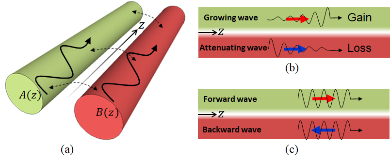
Figure 1: (a) Coupling between two electromagnetic waves whose complex amplitudes are $A$ and $B$. Conditions that lead to EPDs are obtained by introducing proper coupling between: (b) two waveguides with PT symmetry where the two media have gain and loss supporting exponentially growing and attenuating waves; (c) two waveguides with forward and backward propagating waves, without resorting to PT symmetry (i.e., in this case the waveguides do not have gain and loss). The waves with black arrows represent the directions of propagation. The blue and red arrows represent the directions of power flow.

II Second order EPD by mixing two waves

We consider two coupled electromagnetic waves as shown in Fig. 1(a). These two waves are described by the complex time-domain notation

$$\begin{array}[]{c}a(\mathbf{r},t)=A(z)f_{a}(\mathbf{\boldsymbol{\rho}})e^{i\omega t},\\ b(\mathbf{r},t)=B(z)f_{b}(\mathbf{\boldsymbol{\rho}})e^{i\omega t},\end{array}$$ (1)

where $A(z)$ and $B(z)$ are the complex amplitudes of waves along the $z$ direction, $\mathbf{r}=\boldsymbol{\rho}+z\hat{\mathbf{z}}$, and $\boldsymbol{\rho}$ is the transverese coordinate. $f_{a}(\mathbf{\boldsymbol{\rho}})$ and $f_{b}(\mathbf{\boldsymbol{\rho}})$ are the normalized modal field profile in the transverse direction for each mode. When the two waves are uncoupled, i..e., when their waveguides are far from from each other, the evolution of the amplitudes along the $z$ direction is simply descried by $dA(z)/dz=-i\beta_{a}^{\prime}A(z)$ and $dB(z)/dz=-i\beta_{b}^{\prime}B(z)$, where $\beta_{a}^{\prime}$ and $\beta_{b}^{\prime}$ are the uncoupled propagation constants of each wave (that is also an eigenmode of the structure since there is no coupling). The solutions are $A(z)=A_{0}\exp(-i\beta_{a}^{\prime}z)$ and $B(z)=B_{0}\exp(-i\beta_{a}^{\prime}z)$. The power carried by each wave in the positive $z$ direction is given by $p_{a}(z)=\pm|A(z)|^{2}$ and $p_{b}(z)=\pm|B(z)|^{2}$ where the sign depends on the type of the wave. The sign is positive when the wave is forward, i.e., when the power is carried in the same direction of wave propagation (i.e., when the phase and group velocity have the same directions). The sign is negative when the waves backward, i.e., when the phase propagates along the positive $z$ direction whereas the power flows in the negative $z$ direction (i.e., when the phase and group velocity have the opposite directions).

When coupling is introduced to those two waves, the system eigenmode is found by solving the spatial-evolution equation that, based on coupled mode theory [13, 14], is given by

$$\dfrac{d}{dz}\left(\begin{array}[]{c}A(z)\\ B(z)\end{array}\right)=-i\left(\begin{array}[]{cc}\beta_{a}&\kappa_{ab}\\ \kappa_{ba}&\beta_{b}\end{array}\right)\left(\begin{array}[]{c}A(z)\\ B(z)\end{array}\right),$$ (2)

where $\beta_{a}$ and $\beta_{b}$ are “perturbed” propagation constants for the coupled system, and $\kappa_{ab}$ and $\kappa_{ba}$ are the coupling coefficients between the two modes. The relation between $\kappa_{ab}$ and $\kappa_{ba}$ is determined by applying the power conservation principle. The total power carried in the coupled structure is $p_{t}(z)=|A(z)|^{2}\pm|B(z)|^{2}$ assuming wave $A$ is forward wave, and wave $B$ to be either forward or backward, when taking the $+$ or the $-$ sign, respectively. Thus, there are two possible scenarios: (i) “codirectional coupling” when both waves carry power at the same direction and (ii) “contradirectional coupling” when the two waves carry power in the opposite direction [13].

When the system does not have gain and loss, conservation of energy states that $dp_{t}(z)/dz=0$, and by using (2), one finds that the constraint $\mathrm{Re}\left(AB^{*}\left(\kappa_{ba}\mp\kappa_{ab}^{*}\right)\right)=0$ should be satisfied. Therefore, we have $\kappa_{ab}=\kappa_{ba}^{*}$ in case of codirectional coupling where the two waves are forward, and $\kappa_{ab}=-\kappa_{ba}^{*}$ in case of contradirectional coupling where one wave is a forward and the other one is backward [13].

The mixing of the two waves constitutes what is called the guiding system’s eigenmode (some call it “supermode”) which is a weighted sum of the individual guided waves. The eigenmode propagation constant is determined by solving the characteristic equation of the coupled system in (2) assuming the wave amplitudes to be in the form of $[A(z),B(z)]^{T}\propto e^{-ikz}$ which yields $k^{2}-k(\beta_{a}+\beta_{b})+\left(\beta_{a}\beta_{b}-\kappa_{ab}\kappa_{ba}\right)=0.$ The characteristic equation has two solutions that are given by

$$\begin{array}[]{c}k_{n}=\dfrac{\beta_{a}+\beta_{b}}{2}+(-1)^{n}\sqrt{\left(\dfrac{\beta_{a}-\beta_{b}}{2}\right)^{2}-\left(-1\right)^{p}\kappa^{2}},\end{array}$$ (3)

where $\kappa=|\kappa_{ab}|$ and the indices $n=1,2$ denote the two modes of the coupled system. Furthermore, $p=1$ and $p=2$ represent the case of codirectional and contradirectional coupling, respectively. An EPD occurs when two eigenmodes coalesce, i.e., $k_{1}=k_{2}=k_{e},$ with $k_{e}=\left(\beta_{a}+\beta_{b}\right)/2$. This EPD occurs when $\beta_{a}-\beta_{b}=2\sqrt{\left(-1\right)^{p}\kappa^{2}}$. At an EPD, the eigenvectors must coalesce, and in this simple system their coalescence follows from the coalescence of the eigenvalues. Indeed, the two eigenvectors are $\left[\begin{array}[]{cc}A_{n},&B_{n}\end{array}\right]^{T}=\left[\begin{array}[]{cc}1,&(k_{n}-\beta_{a})/\kappa_{ab}\end{array}\right]^{T}$and it is easy to see that they coalesce when $k_{1}=k_{2}$.

The group velocity of the eigenmode with wavenumber $k_{n}$ is determined as (assuming $k_{n}$ to be purley real)

$$v_{g,n}=\frac{1}{d_{\omega}k_{n}}=\dfrac{k_{n}-k_{e}}{2k_{n}d_{\omega}\left(\beta_{a}+\beta_{b}\right)+2d_{\omega}\left(\beta_{a}\beta_{b}+\left(-1\right)^{p}\kappa^{2}\right)}.$$ (4)

where $d_{\omega}\equiv d/d\omega$ denotes the derivative with respect to angular frequency $\omega$. It is clear from the expression that $v_{g,1,2}=0$ when $k_{1}=k_{2}=k_{e},$i.e., exactly at the EPD. Next, we also show what happens near the EPD.

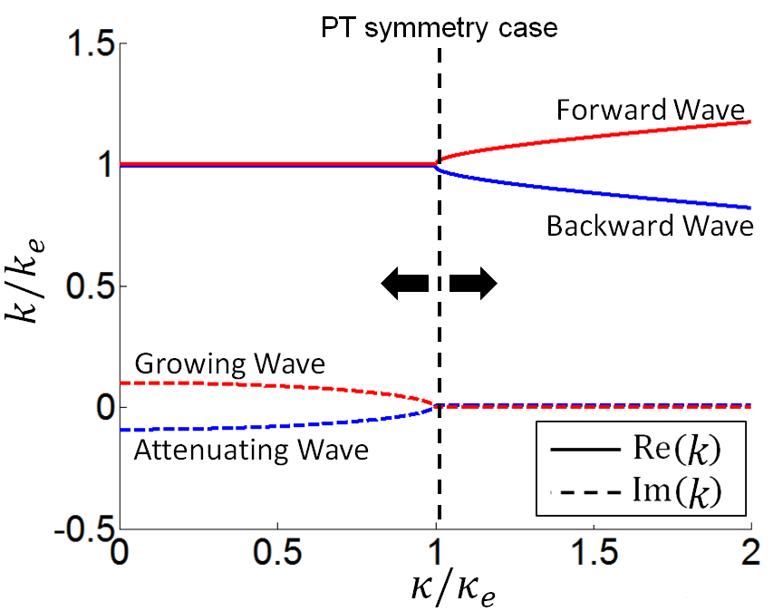
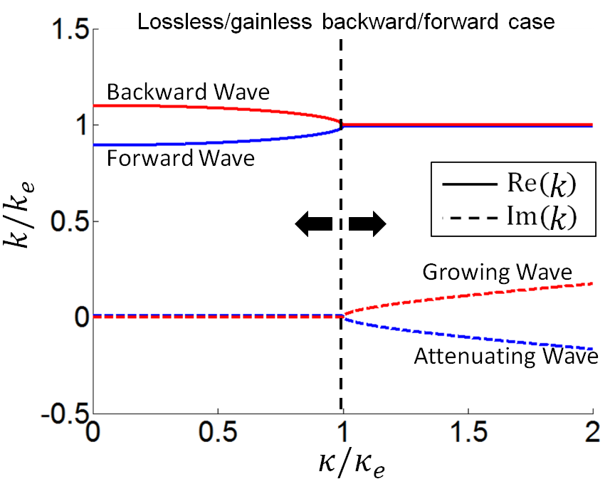
Figure 2: The two wavenumbers of the guiding system versus the coupling parameter $\kappa$, showing the existence of an EPD. Two cases are examined: (a) coalescence of modes in PT-symmetrical waveguides, (b) coalescence of modes obtained by coupling a forward wave (phase and group velocities have the same direction) and a backward wave (phase and group velocities have opposite directions). Both cases exhibit an EPD, represented by the bifurcation point.

II-A Codirectional coupling $(\kappa_{ab}=\kappa_{ba}^{*})$

For the case of codirectional coupling , $p=1,$ the EPD condition is simplified to $\beta_{a}-\beta_{b}=\pm 2i\kappa$. The EPD condition puts a constraint that the difference between the propagation constants of the uncoupled waves has to be purely imaginary in order to exhibit an EPD. Thus, we conclude that the EPD can never be obtained for any value of the coupling parameter $\kappa$ in the case of a lossless/gainless system. If we resort to a PT symmetry, as in Fig. 1(b), where the system has balanced gain and loss, we have $\beta_{a}=\beta_{0}+i\alpha$ and $\beta_{b}=\beta_{0}-i\alpha$, and an EPD is obtained when $\alpha=\kappa$ [9, 10, 11, 16, 17], and the degenerate wavenumber is $k_{e}=\beta_{0}$.

For this case, the two propagation constants of the coupled system in the vicinity of the EPD are $k_{1,2}=\beta_{0}\pm\sqrt{\kappa^{2}-\alpha^{2}}$ and their derivatives are $d_{\omega}k_{1,2}=d_{\omega}\beta_{0}\pm\left(2\kappa d_{\omega}\kappa-2\alpha d_{\omega}\alpha\right)/(k_{2}-k_{1})$. This is also illustrated by determining the eigenvector of the degenerate eigenmode from (2) (for codirectional coupling case where $p=1$) as

$$\begin{array}[]{c}\left(\begin{array}[]{c}A_{e}(z)\\ B_{e}(z)\end{array}\right)=\left(\begin{array}[]{c}1\\ -ie^{-i\mathrm{arg}(\kappa_{ab})}\end{array}\right)e^{-ik_{e}z},\end{array}$$ (5)

and one finds that the total power carried by the degenerate eigenmode is $p_{t}(z)=|A_{e}(z)|^{2}-|B_{e}(z)|^{2}=0$ vanishes, in agreement with the vanishing of the group velocity. In the vicinity of an EPD we have $k_{1}\approx k_{2}$ and by neglecting the $d_{\omega}\beta_{0}$, usually smaller than the other term, the group velocities of the two modes are $v_{g,1,2}\approx\pm\left(k_{2}-k_{1}\right)/\left(2\kappa d_{\omega}\kappa-2\alpha d_{\omega}\alpha\right)$ when $\kappa>\kappa_{e}$, i.e., where the two eigenmodes are propagating with purley real wavenumbers. Therefore we conclude that near an EPD in a PT-symmetric guiding system, the two modes of the coupled system are phase-synchronized ($k_{1}\approx k_{2}$), i.e., with almost identical phase velocity, but have opposite group velocity ($v_{g,1}\approx-v_{g,2}$), which eventually results on having a wave in the guiding structure with vanishing group velocity when the system is exactly at the EPD. As an example, for a system with PT symmetry where the uncoupled waveguides have, respectively, a growing wave with $\beta_{a}=100+10i$ (1/m) and an attenuating wave with $\beta_{b}=100-10i$ (1/m), an EPD is obtained when the coupling parameter is $\kappa=10$ 1/m as shown in Fig. 2(a).

II-B Contradirectional coupling $(\kappa_{ab}=-\kappa_{ba}^{*})$

We consider coupling between forward wave with wavenumber $\beta_{a}>0$ and $v_{g,a}>0$ ($v_{g,a}=d_{\omega}\beta_{a}$) and backward wave with wavenumber $\beta_{b}>0$ and $v_{g,b}<0$ ($v_{g,b}=d_{\omega}\beta_{b}$). The two propagating waves carry power in opposite directions and therefore they exhibit contradirectional coupling, we use $p=2$ in Eq. (3). The EPD condition ($k_{1}=k_{2}$) for this case is simplified to $\beta_{a}-\beta_{b}=\pm 2\kappa$, which means that the difference between the propagation constants should be purely real to have an EPD, which is possible for a lossless/gainless system. Therefore, the EPD condition for this case is satisfied through the proper design of the coupling parameters, i.e, when $\kappa=\left|\beta_{a}-\beta_{b}\right|/2$ (we recall that $\kappa$ was defined as purely real positive). This means that there are two possible EPD conditions, $\beta_{a}-\beta_{b}=2\kappa$ and $\beta_{a}-\beta_{b}=-2\kappa$, that may both occur when varying frequency. At those two frequencies one has $\beta_{a}>\beta_{b}$ and $\beta_{b}>\beta_{a}$, respectively. A more detailed discussion is provided later on when discussing the indirect bandgap.

In the vicinity of an EPD, the two propagation constants of the coupled system are given by Eq. (3), and the derivatives of the two wavenumbers with respect to the angular frequency are

$$d_{\omega}k_{1,2}=\frac{1}{2}d_{\omega}\left(\beta_{a}+\beta_{b}\right)\pm\frac{1}{2}\dfrac{\left(\beta_{a}-\beta_{b}\right)d_{\omega}\left(\beta_{a}-\beta_{b}\right)-2\kappa d_{\omega}\kappa}{(k_{2}-k_{1})}.$$ (6)

When $\kappa<\kappa_{e}$, i.e., where the two eigenmodes are propagating with purely real wavenumbers, in the vicinity of an EPD we have $k_{1}\approx k_{2}$ and by neglecting the term $d_{\omega}\left(\beta_{a}+\beta_{b}\right)$ with respect to the second one, the group velocities of the two modes are

$$v_{g,1,2}\approx\pm\frac{k_{2}-k_{1}}{\frac{1}{2}\left(\beta_{a}-\beta_{b}\right)\left(v_{g,a}^{-1}-v_{g,b}^{-1}\right)-2\kappa d_{\omega}\kappa}.$$ (7)

Therefore, we conclude that near an EPD, the coupled forward and backward waves are syncronised in phase, i.e., $k_{1}\approx k_{2}$ but have nearly opposite group velocity ($v_{g,1}\approx-v_{g,2}$), which eventually results in having a wave in the guiding structure with vanishing group velocity when the system is exactly at an EPD.

This is also illustrated by determining the eigenvector of the degenerate eigenmode from (2) (for contradirectional coupling case where $p=2$) as

$$\begin{array}[]{c}\left(\begin{array}[]{c}A_{e}(z)\\ B_{e}(z)\end{array}\right)=\left(\begin{array}[]{c}1\\ -e^{-i\mathrm{arg}(\kappa_{ab})}\end{array}\right)e^{-ik_{e}z},\end{array}$$ (8)

and one finds that the total power carried by the degenerate eigenmode is $P_{t}(z)=|A_{e}(z)|^{2}-|B_{e}(z)|^{2}=0$ vanishes, in agreement with the vanishing of the group velocity. At the EPD, the system matrix is not diagonalizable but rather similar to a $2\times 2$ Jordan matrix. The fields in the two-waveguide system is represented using the degenerate and generalized eigenvectors as

$$\begin{array}[]{c}\left(\begin{array}[]{c}A(z)\\ B(z)\end{array}\right)=\left(\begin{array}[]{c}1\\ -e^{-i\mathrm{arg}(\kappa_{ab})}\end{array}\right)\left(u_{1}-jzu_{2}\right)e^{-ik_{e}z}\\ \ \ \ \ \ \ \ \ \ \ \ \ \ \ +\left(\begin{array}[]{c}1\\ ie^{-i\mathrm{arg}(\kappa_{ab})}/\kappa_{e}\end{array}\right)u_{2}e^{-ik_{e}z}.\end{array}$$ (9)

where $u_{1}$ and $u_{2}$ are proper coefficients that depend on the system excitation and boundary conditions.

The two waveguides with contradirectional coupling are schematically shown in Fig. 1(c) and the dispersion diagram is in Fig. 2 where we see a forward wave with $\beta_{a}=110$ (1/m) and backward wave with $\beta_{b}=90$ (1/m), and the EPD is obtained at $k=k_{e}=100$ (1/m) , where $\kappa_{e}=10$ (1/m) as shown in Fig. 2(b).

The contradirectional coupling case can be realized is in two possible scenarios: (i) two modes exist in two separate waveguides where the first waveguide supports a forward wave and the second waveguide supports a backward wave and the coupling is introduced by bringing them near each other; (ii) two modes exist in the same waveguide having periodicity where the one wave (e.g., the forward) has the fundamental Floquet harmonic equal to $\beta_{1}=\beta_{0}$ and the other wave (e.g., the backward) has its 1st harmonic Floquet harmonic equal to $\beta_{2}=-\beta_{0}+2\pi/d$, where $d$ is the waveguide period, and the EPD is only possible at the band edge $\beta_{0}=\pi/d$. An example belonging to the first scenario, where the EPD is found in two coupled dielectric slab waveguides, is shown later on. The second scenario instead exists in conventional periodic waveguides and it is not further considered in this paper.

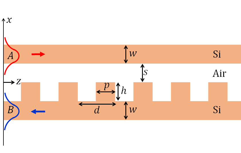
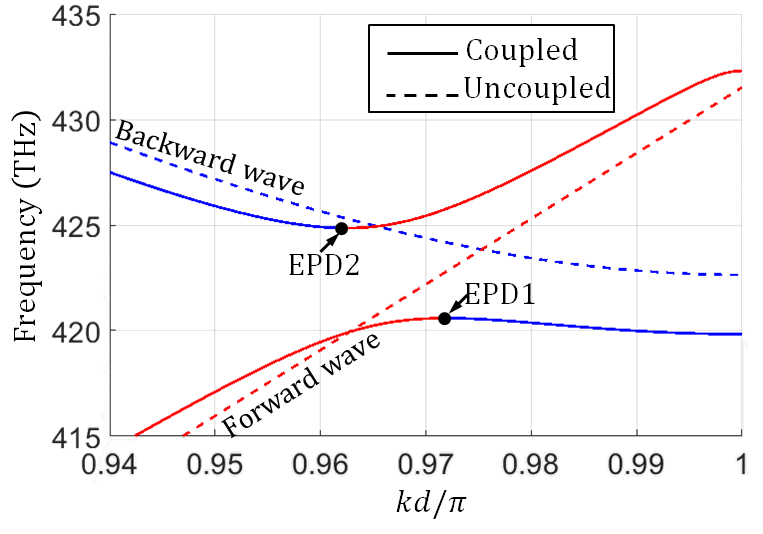
Figure 3: Example of modal EPD of order 2 between a forward wave (phase and group velocities have the same direction) and backward wave (phase and group velocities have opposite directions). (a) Two coupled Si layers where the top one supports a forward wave (in red) while the bottom one is periodically corrugated to support a backward wave (positive phase velocity and negative group velocity, in blue). The red and blue arrows represent the direction of power flow. (b) Dispersion relation showing the propagating eigenmodes when the two waveguides are uncoupled (dashed) and when the are coupled (solid). The dispersion of modes in the coupled waveguides show the existence of two EPDs. The blue and red colors of the curves are related to the power flow directions. Note also that because two EPDs are found, an indirect bandgap is present between the upper and lower branches that can be designed ad-hoc. In the shown case we have $\Delta k_{e}\equiv k_{e2}-k_{e1}<0$.

We present an example of a guiding system that supports two waves carrying power in opposite directions and we show that it exhibits two EPDs. Consider the guiding system made of a Si substrate (supporting the forward wave) coupled to a Si grating waveguide as shown in Fig. 3, with dimensions $w=p=h=70$ nm and $d=140$ nm. Silcon is modeled with a refractive index $n_{\mathrm{Si}}=3.45$. We first show in Fig. 3 the dispersion of the two wavenumbers $\beta_{a}^{\prime}$ and $\beta_{b}^{\prime}$ of the two uncoupled waveguides ($s\to\infty$) as red dashed (uniform waveguide) and blue dashed (grating waveguide). The figure shows that the structures support a forward wave where the group velocity is positive $v^{\prime}_{g,a}=1/(d_{\omega}\beta_{a}^{\prime})>0$ and a backward wave where the group velocity is negative $v^{\prime}_{g,b}=1/(d_{\omega}\beta_{b}^{\prime})<0$. In the same Fig. 3, we show the dispersion of the two wavenumbers $k_{1}$ and $k_{2}$ of the coupled guiding system, i.e., when the two waveguide are close to each other with a gap of $s=70$ nm. The dispersion show the existence of two EPDs associated to a wavenumber (momentum) displacement. The dispersion diagrams we show are for modes with electric field polarized in the $y$ direction. The dispersion diagrams have been found by using the finite element method-based eigenmode solver implemented in CST Studio Suite, by numerically simulating only one unit cell of the structure. The proposed condition allows to locate the EPDs at band edges that are not necessarily at the center or at the edge of a Brillioum zone, without using loss and gain. It also shows the capability to engineer an indirect bandgap in these simple structures.

III Indirect bandgap in the contradirectional case

Figure 4: Schematic of a dispersion diagram showing the indirect bandgap that results from two EPDs based on contradirectional coupling. The red-dashed line represents the wavenumber of the forward wave $\beta_{a}^{\prime}$ whereas the blue-dahsed line the one of the backward wave $\beta_{b}^{\prime}$, when the waveguides are uncoupled. The coupling yields the two curves with two EPDs that are labeled as EPD1 and EPD2. The indirect bandgap width is $\Delta\omega_{IB}$. In the shown case $\Delta k_{e}\equiv k_{e2}-k_{e1}>0$.

In the contradirectional case where coupling occurs between a forward and backward wave, as in Fig. 1(c), an indirect bandgap is possible and we show here how it is formed. Since in this case one wave is forward and one is backward, the uncoupled propagation constants $\beta_{a}^{\prime}$ and $\beta_{b}^{\prime}$ have opposite slopes as schematically shown in Fig. 4 (see also dashed blue and red curves in Fig. 3), and an analogous trend is expected for the parameters $\beta_{a}$ and $\beta_{b}$ of the coupled system. By looking at the dispersion diagram shown in Fig. 4, the red-dashed curve is the forward wave with wavenumber $\beta_{a}^{\prime}(\omega)$ and the blue-dashed curve is the backward wave with wavenumber $\beta_{b}^{\prime}(\omega)$. Assuming that the coupling it not so strong, one may assume that $\beta_{a}(\omega)\approx\beta_{a}^{\prime}(\omega)$ and $\beta_{b}(\omega)\approx\beta_{b}^{\prime}(\omega)$, at least in trend, hence, in slope. The forward wave has positive slope, $v_{g,a}=d\omega/d\beta_{a}>0$, whereas the backward wave has negative slope $v_{g,b}=d\omega/d\beta_{b}<0$, and the dispersion curves for $\beta_{a}$ and $\beta_{b}$ versus frequency should intersect at some frequency ($\beta_{a}=\beta_{b}$) because one wavenumber is increasing with frequency whereas the other is decreasing with frequency; an example with a grating is illustrated in Fig. 3 while a schemtic is in Fig. 4. Let us approximate the dispersion curves locally, in the frequency range of interest, as straight lines, i.e., $\beta_{a}(\omega)\approx a+v_{g,a}^{-1}\omega$ and $\beta_{b}(\omega)\approx b+v_{g,b}^{-1}\omega$, where now $v_{g,a}$ and $v_{g,b}$ are assumed to have the local fixed value. Furthermore, assuming, for simplicity, that $\kappa$ is constant within the frequency range of interest, one finds that EPDs occurs at two angular frequencies $\omega_{e1}$ and $\omega_{e2}$ such that $\beta_{a}(\omega_{e1})-\beta_{b}(\omega_{e1})=-2\kappa$ and $\beta_{a}(\omega_{e2})-\beta_{b}(\omega_{e2})=2\kappa$, where $\omega_{e1}<\omega_{e2}$. Subtracting the previous two conditions leads to the indirect bandgap determination

$$\Delta\omega_{IB}\equiv\omega_{e2}-\omega_{e1}\approx\frac{4\kappa}{v_{g,a}^{-1}-v_{g,b}^{-1}}.$$ (10)

Note that $v_{g,a}^{-1}-v_{g,b}^{-1}>0$, hence $\Delta\omega_{IB}>0$. The bandgap width can be controlled by the slope of the two parameters $\beta_{a}$ and $\beta_{b}$; indeed, when $v_{g,a}^{-1}\approx-v_{g,b}^{-1}$, the denominator of (10) is small and the bandgap is very wide, viceversa, the bandgap is narrow when $v_{g,a}^{-1}$ is very different from $-v_{g,b}^{-1}$. If we consider the dispersion of the coupling term $\kappa$, a more complicated picture may arise that could be determined by the reasoning just provided.

The degenerate wavenumbers at the two EPDs are $k_{e,1}=\left(\beta_{a}(\omega_{e1})+\beta_{b}(\omega_{e1})\right)/2$ and $k_{e,2}=\left(\beta_{a}(\omega_{e2})+\beta_{b}(\omega_{e2})\right)/2$. Using the linear approximation formulas for the wavenumbers $\beta_{a}(\omega)$ and $\beta_{a}(\omega)$, one finds that $k_{e1}\approx[a+b+\left(v_{g,a}^{-1}+v_{g,b}^{-1}\right)\omega_{e1}]/2$ and $k_{e2}\approx[a+b+\left(v_{g,a}^{-1}+v_{g,b}^{-1}\right)\omega_{e2}]/2$ . The difference between the two degenerate wavenumbers is

$$\Delta k_{e}\equiv k_{e2}-k_{e1}\approx\frac{v_{g,a}^{-1}+v_{g,b}^{-1}}{2}\Delta\omega_{IB}.$$ (11)

Therefore, it is necessary that $v_{g,a}^{-1}+v_{g,b}^{-1}\neq 0$ in order to have indirect bandgap. When $|v_{g,a}^{-1}|>|v_{g,b}^{-1}|$ we get $k_{e2}>k_{e1},$hence $\Delta k_{e}>0$, i.e., the EPD that occurs at the smaller frequency $\omega_{e1}$ occurs also at the smaller degenerate wavenumber $k_{e1}$ and this condition is depicted in Fig. 4. When $|v_{g,a}^{-1}|<|v_{g,b}^{-1}|$, we get $k_{e1}>k_{e2},$ hence $\Delta k_{e}<0$, i.e., the EPD that occurs at the smaller frequency $\omega_{e1}$ occurs at larger degenerate wavenumber $k_{e1}$ and this condition is depicted in Fig. 3. Indeed, by looking at Fig. 3, one finds by naked eye that $|v_{g,a}|>|v_{g,b}|$ , (absolute change with frequency of dashed red curve is higher than the one of the dashed blue one), therefore $|v_{g,a}^{-1}|<|v_{g,b}^{-1}|$ resulting in $k_{e1}>k_{e2}$ according to (11) and the EPD at lower frequency, around 420 THz, occurs at higher degenerate wavenumber of $k_{e1}=0.972\,\pi/d$ .

IV Conclusion

We have demonstrated that EPDs are not only obtained in PT-symmetric waveguides but they are also obtained in two lossless and gainless waveguides when they support forward and backward waves that are properly coupled. We have shown a simple system that supports this condition made of a grating (supporting a backward guided mode) coupled to a dielectric layer (supporting the forward mode). We have elaborated that the scheme discussed here exhibits a photonic indirect bandgap that can be controlled by changing the group velocities of the forward and backward modes along with the coupling coefficient. Two conditions may occur: the bandgap is associated either to a positive or negative momentum difference between the two energy levels. The finding in this paper can be useful to design systems with EPDs whose use is of growing importance for enhancing light-matter interactions and nonlinear photonic phenomena.

References

- [1] M. I. Vishik and L. A. Lyusternik, “The solution of some perturbation problems for matrices and selfadjoint or non-selfadjoint differential equations i,” Russian Mathematical Surveys, vol. 15, pp. 1–73, jun 1960, doi: 10.1070/rm1960v015n03abeh004092.
- [2] P. Lancaster, “On eigenvalues of matrices dependent on a parameter,” Numerische Mathematik, vol. 6, pp. 377–387, dec 1964, doi: 10.1007/bf01386087.
- [3] A. P. Seyranian, “Sensitivity analysis of multiple eigenvalues,” Journal of Structural Mechanics, vol. 21, pp. 261–284, jan 1993, doi: 10.1080/08905459308905189.
- [4] T. Kato, Perturbation Theory for Linear Operators. Springer-Verlag New York Inc., New York, 1966, doi: 10.1007/978-3-662-12678-3.
- [5] C. M. Bender and S. Boettcher, “Real spectra in non-Hermitian Hamiltonians having PT symmetry,” Physical Review Letters, vol. 80, no. 24, p. 5243, 1998.
- [6] C. M. Bender, “Making sense of non-hermitian hamiltonians,” Reports on Progress in Physics, vol. 70, no. 6, p. 947, 2007.
- [7] A. Mostafazadeh, “Exact pt-symmetry is equivalent to hermiticity,” Journal of Physics A: Mathematical and General, vol. 36, no. 25, p. 7081, 2003.
- [8] V. S. Asadchy, M. S. Mirmoosa, A. Díaz-Rubio, S. Fan, and S. A. Tretyakov, “Tutorial on electromagnetic nonreciprocity and its origins,” Proceedings of the IEEE, vol. 108, no. 10, pp. 1684–1727, 2020.
- [9] A. Ruschhaupt, F. Delgado, and J. Muga, “Physical realization of-symmetric potential scattering in a planar slab waveguide,” Journal of Physics A: Mathematical and General, vol. 38, no. 9, p. L171, 2005.
- [10] R. El-Ganainy, K. Makris, D. Christodoulides, and Z. H. Musslimani, “Theory of coupled optical PT-symmetric structures,” Optics Letters, vol. 32, no. 17, pp. 2632–2634, 2007.
- [11] A. Guo, G. Salamo, D. Duchesne, R. Morandotti, M. Volatier-Ravat, V. Aimez, G. Siviloglou, and D. Christodoulides, “Observation of p t-symmetry breaking in complex optical potentials,” Physical Review Letters, vol. 103, no. 9, p. 093902, 2009.
- [12] M. V. Berry, “Physics of nonhermitian degeneracies,” Czechoslovak Journal of Physics, vol. 54, no. 10, pp. 1039–1047, 2004.
- [13] A. Yariv, “Coupled-mode theory for guided-wave optics,” IEEE Journal of Quantum Electronics, vol. 9, no. 9, pp. 919–933, 1973.
- [14] A. Hardy and W. Streifer, “Coupled mode theory of parallel waveguides,” Journal of lightwave technology, vol. 3, no. 5, pp. 1135–1146, 1985.
- [15] T. Mealy and F. Capolino, “General conditions to realize exceptional points of degeneracy in two uniform coupled transmission lines,” IEEE Transactions on Microwave Theory and Techniques, vol. 68, no. 8, pp. 3342–3354, 2020.
- [16] Y. Li, X. Guo, L. Chen, C. Xu, J. Yang, X. Jiang, and M. Wang, “Coupled mode theory under the parity-time symmetry frame,” Journal of Lightwave Technology, vol. 31, no. 15, pp. 2477–2481, 2013.
- [17] M. A. Othman and F. Capolino, “Theory of exceptional points of degeneracy in uniform coupled waveguides and balance of gain and loss,” IEEE Transactions on Antennas and Propagation, vol. 65, no. 10, pp. 5289–5302, 2017.