IRB-NLP at SemEval-2022 Task 1: Exploring the Relationship Between Words and Their Semantic Representations

Abstract

What is the relation between a word and its description, or a word and its embedding? Both descriptions and embeddings are semantic representations of words. But, what information from the original word remains in these representations? Or more importantly, which information about a word do these two representations share? Definition Modeling and Reverse Dictionary are two opposite learning tasks that address these questions. The goal of the Definition Modeling task is to investigate the power of information laying inside a word embedding to express the meaning of the word in a humanly understandable way – as a dictionary definition. Conversely, the Reverse Dictionary task explores the ability to predict word embeddings directly from its definition. In this paper, by tackling these two tasks, we are exploring the relationship between words and their semantic representations. We present our findings based on the descriptive, exploratory, and predictive data analysis conducted on the CODWOE dataset. We give a detailed overview of the systems that we designed for Definition Modeling and Reverse Dictionary tasks, and that achieved top scores on SemEval-2022 CODWOE challenge in several subtasks. We hope that our experimental results concerning the predictive models and the data analyses we provide will prove useful in future explorations of word representations and their relationships.

1 Introduction

The COmparing Dictionaries and WOrd Embeddings (CODWOE) task Mickus et al. (2022) is aimed at explaining two different types of semantic descriptions of words: dictionary glosses and word embeddings. A dictionary gloss is a brief textual explanation of a word and a word embedding is a vector representation that captures the word’s semantic and syntactic properties Smith (2020).

In order to investigate the relationship between these two types of descriptions, two complementary subtracks were put together: 1. Definition Modeling(DEFMOD) track, where correct glosses need to be generated from word embedding vectors Noraset et al. (2017); and 2. Reverse Dictionary(REVDICT) track, where correct embedding vectors should be generated from dictionary glosses Hill et al. (2016). The datasets for both tracks cover five different languages: English (EN), Spanish (ES), French (FR), Italian (IT), and Russian (RU).

The key challenge of the CODWOE task is that it needs to be performed without external data, which precludes the use of pretrained models and vectors. Additionally, the training dataset is relatively small in comparison to the datasets on which models are typically trained.

Our strategy was to adapt an RNN-based decoder model Noraset et al. (2017) for the DEFMOD track, and to use a transformer-based encoder Devlin et al. (2019) for the REVDICT track. With the limited amount of available data in mind, we hypothesized that models should not be large. Therefore we aimed to limit the model complexity by reducing the number of parameters, for example by using a subword tokenizer Kudo and Richardson (2018), which yields a smaller dictionary of optimized subword fragments. All of the models we used were built for a single language, and their structure and parameters were optimized either iteratively or by way of Bayesian hyperparameter optimization (BHO) Snoek et al. (2012).

We conducted data analyses of the CODWOE datasets and analyses of the developed machine learning models. We performed a statistical and visual analysis of the pretrained CODWOE embeddings, i.e., of their distributions and relationships. DEFMOD analyses include an analysis of model performance factors and a qualitative analysis of generated glosses. In the REVDICT predictive analysis, we investigate the impact of many different settings on models’ performance defined in terms of distance and similarity scores between predicted and target vectors.

We show that our adaptation of the DEFMOD architecture Noraset et al. (2017) can perform competitively and that the use of multiple word embeddings can clearly improve the generation of word glosses. For REVDICT, we demonstrate that our approaches achieve top performance in terms of ranking, which makes them suitable for information retrieval applications. Our models perform competitively and our results on the CODWOE challenge can be found in Table 1. We make the code of our models and data analyses publicly available.

Table 1: Aggregated language-level ranks of our team for the DEFMOD (DM) and REVDICT (RD) tracks (and the number of teams competing in a subtask).

TASK	EN	ES	FR	IT	RU
DM-all	2 (9)	1 (7)	1 (6)	5 (7)	5 (6)
RD-sgns	3 (9)	1 (7)	1 (6)	1 (7)	2 (6)
RD-char	4 (7)	3 (5)	4 (5)	2 (6)	2 (5)
RD-electra	5 (6)		3 (4)		3 (4)

2 Background

2.1 Related Work

Definition Modeling

The Definition Modeling (DEFMOD) task, first introduced in Noraset et al., 2017, is focused on the prediction of dictionary word glosses from word embeddings. Noraset et al. (2017) experimented on two English dictionaries and proposed a successful architecture based on RNN.

Subsequent work on Definition Modeling focused on variations of the problem of prediction of a word gloss from the word sense. These approaches consider gloss prediction based on sense-specific word embeddings Gadetsky et al. (2018); Kabiri and Cook (2020); Zhu et al. (2019), and on a word-based context indicating the word sense Gadetsky et al. (2018); Mickus et al. (2019); Bevilacqua et al. (2020); Zhang et al. (2020); Yang et al. (2020). The proposed approaches are based either on RNNs Gadetsky et al. (2018); Kabiri and Cook (2020); Zhu et al. (2019); Zhang et al. (2020) or Transformers Mickus et al. (2019); Bevilacqua et al. (2020). All of the previous approaches rely on word embeddings pre-trained on large corpora, most commonly word2vec Mikolov et al. (2013). Sense-aware approaches that take embeddings as input make use of either sense-aware word embeddings Gadetsky et al. (2018); Kabiri and Cook (2020) or of decomposition of word embeddings into sense-specific vectors Zhu et al. (2019).

The initially proposed architecture of Noraset et al. (2017) is often used as a baseline solution. The most commonly used measure of model performance is the BLEU Papineni et al. (2002) metric. Although there is some overlap in used datasets, most experiments rely on a specific dataset. The reported model performances vary greatly. Noraset et al. (2017) report BLEU of $31$ and $23$, depending on the dictionary. Subsequent experiments report, for the same approach, BLEU scores that range from as little as $11$ Gadetsky et al. (2018) to as much as $60$ Kabiri and Cook (2020). The variation can be great even for the same language and experimental setup Kabiri and Cook (2020). The original approach of Noraset et al. (2017) remains competitive in the sense-aware setting, with the sense-aware approaches achieving BLEU increases that range between $1-2$ Gadetsky et al. (2018); Kabiri and Cook (2020); Zhang et al. (2020) and $5-6$ Yang et al. (2020); Kabiri and Cook (2020); Zhang et al. (2020), depending on the setting.

While we view the Definition Modeling primarily as a theoretically interesting task, potential applications include explainability of word embeddings and automatic generation of dictionaries, which might be of interest in low-resource settings.

Reverse Dictionary

The Reverse Dictionary (REVDICT) is a task of finding the right word when a word description is given Dutoit and Nugues (2002); Bilac et al. (2004); Zock and Bilac (2004). It is the formulation of the tip-of-the-tongue problem (TOT) Brown and McNeill (1966) that occurs during text synthesis. It is a condition in which a person knows a lot about the word, such as its meaning and origin, but is unable to recall it. REVDICT is a complex task. There are countless variations of input definitions that should lead to the same one-word concept. This complexity comes in part from the representation of the one-word concepts in the human mind. People tend to relate concepts on the conceptual and lexical level and form a highly connected network of abstractions Zock and Bilac (2004).

Therefore, a natural approach to solving REVDICT is to form a semantic network with nodes (one-word concepts) and edges (associations) to search for the target word Zock and Bilac (2004); Thorat and Choudhari (2016). REVDICT can be realized directly by comparing the input definitions with all the definitions in the dictionary and returning the most similar ones, without taking into account any semantic or grammatical information El-Kahlout and Oflazer (2004). However, REVDICT systems that include semantics give better results, such as in Méndez et al., 2013 and Calvo et al., 2016 where words are represented as vectors in a semantic space.

Recent REVDICT approaches utilize deep learning (DL) to map arbitrary-length definition phrases to the vector representation of the target word Hill et al. (2016); Qi et al. (2020); Yan et al. (2020); Malekzadeh et al. (2021). The success of DL approaches indicates that REVDICT can be solved implicitly, i.e. by directly learning from given data, and doesn’t require an explicit injection of domain knowledge. According to this observation, the DL approach is a good choice for solving the REVDICT task.

2.2 Dataset

The CODWOE datasets Mickus et al. (2022) cover five languages (EN, ES, FR, IT, RU) and are derived from the Dbnary lexical data. Each data point corresponds to a single word and contains word embedding vectors and the word gloss. Three types of embedding are used, labeled as sgns (pretrained word2vec), electra (contextual pretrained embeddings) and char (character-based embeddings). Pretrained embeddings are based on large corpora containing approximately 1B tokens.

Each dataset is divided into three sections: training, validation (development), and test. Datasets for training and validation have 43.608 and 6.375 samples, respectively. Each track also has a separate set of test data. The DEFMOD test dataset has 6.221 samples while the REVDICT has 6.208 samples.

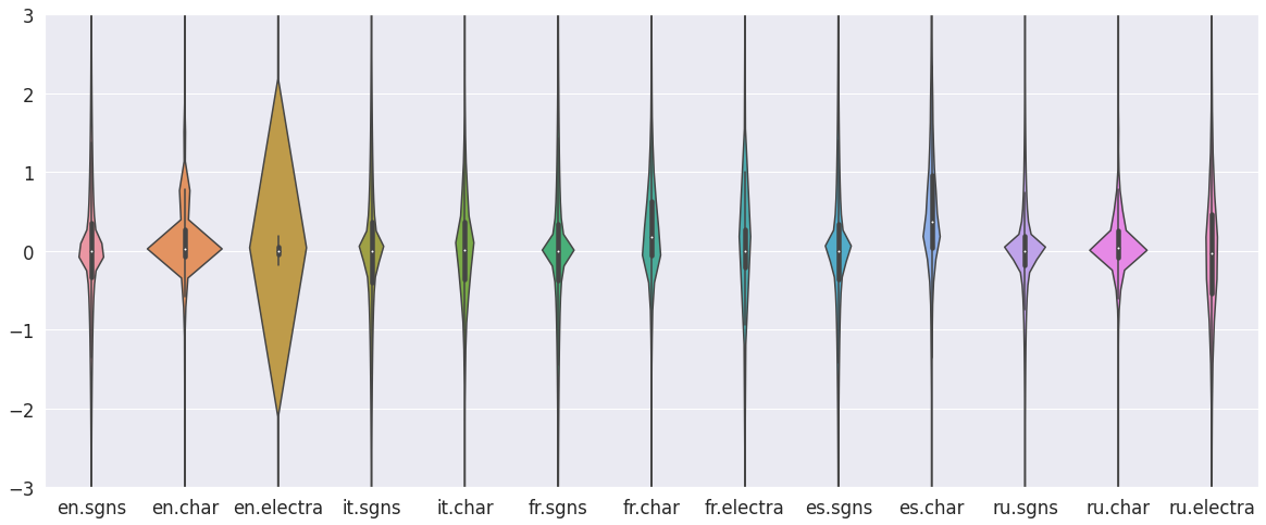
Figure 4: Distributions of vector elements in train datasets within the interval [-3,3].

More detailed statistics and analyses of the dataset can be found in the Appendices, including the gloss statistics (Table 5) and embedding vector statistics (Table 11). Descriptive analysis of the embedding vectors shows large variation in values that depend on a language and an embedding type (Figures 3 and 4). Additionally, an exploratory analysis showed that the embeddings for different languages are easily separable (Figures 6 and 5). Interestingly, patterns of vector-based word similarity seem to differ significantly across embedding types, and in this regard there are no visible relations between different embeddings (Figure 7).

3 System overview

Both the DEFMOD and the REVDICT models rely on unigram subword tokenizers Kudo (2018) trained on glosses from the train datasets.

3.1 Definition Modeling

Our approach to the challenging task of Definition Modeling on a limited dataset consists of preprocessing the input data, extracting the semantic information from the dataset, and controlling the model size and complexity.

The inspection of the learning data revealed that the gloss texts are often long since they consist of several alternative definitions. We opted to include only one definition per learning example. Our intuition is that this approach, also taken in Noraset et al. (2017), alleviates the learning problem by inducing the model to learn shorter and atomic definitions. The approach should also reduce noise (since the number of alternative definitions in a gloss is arbitrary).

The inspection of glosses also revealed the presence of lexicographic labels that precede the gloss definitions. These labels, present for all languages except English, convey data about, for example, word semantics (ex. geography, history) or temporal category (ex. archaic). We chose to remove these labels since they introduce noise (the presence and the amount of labels appears arbitrary), increase the dictionary size, and thus make the learning problem harder.

To construct the dictionary we use the unigram subword tokenizer Kudo (2018) implemented as part of the SentencePiece tool Kudo and Richardson (2018). The reasons for using the subword tokenization were the expected improvement in performance for low-resource tasks Kudo (2018) and the reduction in the number of model parameters corresponding to token embeddings.

Since we opted for a deep learning model depending on token embeddings, we initialized the token embeddings with GloVe vectors Pennington et al. (2014) trained on the dataset of normalized and cleaned atomic glosses. To demonstrate that the GloVe vectors capture a degree of word semantics, we aggregated the vectors on a gloss level using tf-idf weighting. Then we inspected, for each “target” gloss from a sample of English glosses, other dataset glosses ordered by cosine similarity to the target. This revealed that GloVe similarity corresponds to the similarity in gloss meaning. Additionally, we found that the models initialized with GloVe vectors achieve a lower final loss.

Machine learning model

We decided to use an adaptation of the RNN-based model of Noraset et al. (2017), that proved competitive in a number of experimental settings. In the context of the DEFMOD task, the model takes as input one or more word embeddings (sgns, electra or char) and produces a gloss (a sequence of tokens) that should correspond to the word’s correct gloss.

From the input embeddings, we form two vectors, the seed vector $s$ that is used to initialize the RNN, and the context vector $c$. For both the seed and the context vectors we consider using a single embedding, concatenation of embeddings, and a nonlinear transformation of the concatenation. At each position in the sequence the context vector is passed as input, together with the RNN’s output, to the special GRU-like gated cell Noraset et al. (2017). The output of the gated cell is then transformed (via linear transformation and softmax activation) to produce token-level probabilities. The gated cell can learn to effectively combine the semantic context with the RNN-level features in guiding the generation process Noraset et al. (2017). The network architecture we use is labeled as S+G in Noraset et al. (2017).

The described model performs conditional generation of tokens in a sequence, which is a standard approach in RNN-based language modeling. The probability of a gloss $g$ is factorized under the assumption that each token $g_{i}$ depends on the previous tokens, the seed embbedding $s$, and the context $c$ :

$$p(g|s,c)=\prod\limits_{i=1}^{|g|}p(g_{i}|g_{0:i-1},s,c)$$

In Noraset et al. (2017), the context is equal to the seed, i.e., the input word embedding. In our case, both the seed and the context can either be a single embedding or a function of multiple embeddings. This approach enables us to leverage the information from several word embeddings in a flexible way. For example, sgns embeddings can be used as a seed while the context can be formed by passing all the embeddings through a multilayer perceptron. Another important difference is that we use the unigram subword tokenization Kudo (2018). Finally, we experiment with using both LSTM and GRU as the network’s RNN components.

3.2 Reverse Dictionary

We approach REVDICT as a supervised vector regression task and employ an end-to-end deep learning solution. Our model is based on a transformer architecture Vaswani et al. (2017) used as a definition sentence encoder, and a fully connected feed-forward network used as an output regression module.

The transformer is used to produce useful representations from given inputs, where the inputs are tokenized definition sentences. For each subword token in the input sequence, the transformer gives a representation in the form of a vector. Our REVDICT systems implement three different approaches for aggregating the output vectors produced by the transformer: 1. sum, where we sum the representations given for each token in the input sequence; 2. average, where we average the representations given for each token in the input sequence; and 3. eos, where we use only the representation of the last token in the input sequence, i.e. end-of-sequence (eos) token. The output module further transforms these representations into word embedding vectors.

Additionally, we utilize a multi-task learning Caruana (1997); Ruder (2017) approach. To support multi-task learning, we implemented multiple output regression modules that simultaneously predict different types of embedding vectors from the same representations produced by a single encoder. Multi-task learning is used during the model training phase and only output from one output module makes final predictions. The motivation for using a multi-task learning approach is to benefit from inductive transfer between tasks that could improve the results of predicting a single task Caruana (1997).

4 Model Selection and Experimental Setup

In this section we describe the technical details of data preprocessing and model selection that comprise our methods of constructing the DEFMOD and REVDICT models. The conceptual description of the methods is given in Section 3.

4.1 Definition Modeling

Our choices regarding the technical details of data preprocessing and model construction were guided by what we will call development experiments. These experiments consisted of training the model on the train set, and observing both the final development set loss and the quality of the produced glosses.

Output gloss quality was assessed using a separate “trial” dataset - a small dataset of $200$ items provided by the organizers, containing gloss information consisting of the embedding vector, the original word, and the gloss text. The assessment was performed for English glosses only and aimed to assess the quality of the generated text, and the similarity of the output and the original glosses. A choice was deemed an improvement if it led to the improvement of development loss and either improved the generated glosses or caused no degradation in gloss quality. The development of the final algorithm was performed iteratively and heuristically. However, the overall improvement over the iterations is confirmed by the results of the test set evaluations.

Dataset transformation

The transformation of the original dataset is performed by creating unambiguous training examples and removing the uninformative data that makes the problem harder.

In the original dataset a gloss definition often consists of several equivalent but differently phrased definitions. We divided the dictionary glosses into atomic definitions by splitting the text strings around the “;” character. This heuristic was motivated by gloss sample analysis and the inspection of a sample of atomic glosses revealed that it works in the majority of cases. Each atomic gloss in the new dataset was paired with all the embedding vectors of the original gloss.

In order to remove lexicographical labels from the beginning of the glosses’ text, simple language-specific regular expressions and removal rules were formed based on gloss sample analysis. This approach proved to be effective for a large majority of glosses.

To perform further normalization we additionally lowercased all the glosses and removed the punctuation from the end of texts. The code used to preprocess the original dataset, the new dataset, and the transformation log can be found in the code repository. We note that both the SentencePiece dictionary and the GloVe vectors used for DEFMOD are derived from the transformed dataset. The statistics of the transformed glosses are presented in Table 6

Dictionary

We used the unigram subword tokenizer Kudo (2018) available as part of the SentencePiece tool Kudo and Richardson (2018). and trained it using the default parameters. Experiments in Gowda and May (2020) suggest that a vocabulary of $8000$ subwords is a good default choice for several languages in the case of machine translation. Additionally, our development experiments showed that English models using a vocabulary of $8000$ subwords are superior to $10000$ subword models. Therefore we decided to set the number of unigram tokens to $8000$ in case of English, and to $8500$ in case of other, highly inflected languages expected to have a higher number of distinct suffixes.

Pretrained token embeddings

GloVe embeddings Pennington et al. (2014) of the subword tokens, introduced to initialize the tokens with corpus-level semantic information, were constructed as follows. The model was trained on the set of transformed glosses, and the embedding size was fixed to $256$ (the size of the gloss embeddings). The number of training iterations was set to $50$, the “cutoff” parameter $x_{max}$ was set to $10$, while all the other parameters retained their default values. No frequency-based vocabulary pruning was performed.

Machine learning model

We fixed the maximum sequence length of the RNN models to $64$ subword tokens. Our intuition is that this alleviates the learning problem and could lead to models focused on generating shorter but more correct glosses.

The models were optimized using the AdamW algorithm Loshchilov and Hutter (2017) and the standard categorical cross-entropy loss. The training process was stopped after a fixed number of epochs, or if the best solution did not improve by more than $0.1\%$ over $10$ epochs. During inference, the optimal solution was constructed using the beam search algorithm implementation provided by the competition organizers.

We iteratively improved the models using the described development experiments, i.e., relying on the development set loss and analysis of model glosses produced for the trial dataset. We experimented with several architectural elements and hyperparameters: the formulation of the seed (RNN init. value) and context (gate input) of the network, RNN cell type, dropout, learning rate (LR) and LR scheduler, and the number of training epochs.

The most successful variant is constructed by using the concatenation of all the gloss embeddings as the context and the sgns embedding as the seed. This variant uses input dropout of $0.1$ and network dropout of $0.3$. The input dropout is applied to the seed and context vectors, as well as to the word embeddings. The network dropout is applied to the output of the RNN (final layer) and to the output of the gate cell. The chosen learning rate is $0.001$, and the “plateau” LR scheduler is used – LR is multiplied by $0.1$ if there is no improvement over $5$ epochs.

For the context vector, we tried single embeddings and the combined embeddings merged via a multilayer perceptron. Both variants proved inferior to the concatenation of all vectors. The merged seed vector proved no different from the single embedding seed, so we opted for the simpler solution. Both the development experiments and the results showed no difference between the LSTM and the GRU cell.

Analysis of errors revealed that models sometimes produce a deformed output (very short or non-alphabetic string), and that this almost never occurs simultaneously for two distinct models. Therefore a way of heuristic model improvement is to combine it with another fallback model to be used in case of deformed outputs. We combined a model with a concatenated context and a model with a single-embedding context, or two models with distinct RNN cell types. A more detailed analysis of the model variants can be found in Appendix A.2.

Table 2: Characteristics of our REVDICT (RD) approaches (BS = batch size; ME = max epochs; HP = hyperparameter optimization points; S = scheduler; L = loss; MT = multi-task learning).

RD	BS	ME	HP	S	L	MT
1	1024	20	30	CS	MSE	no
2	2048	20	30	CS	MSE	no
3	4096	20	30	CS	MSE	no
4	8192	20	30	CS	MSE	no
5	2048	150	10	PS	MSE	no
6	2048	150	10	PS	MSE	yes

Table 3: Results for the IRB-NLP team systems on the DEFMOD task. MoverScore, BLEU, and lemma-BLEU results are given for each of the five languages. Best result across all teams and models is given, followed by the results of our two best systems. Overall best results of our team are bolded and the rankings can be found in Table 1.

	EN			ES			FR			IT			RU
	MVR	BLEU	lBLEU	MVR	BLEU	lBLEU	MVR	BLEU	lBLEU	MVR	BLEU	lBLEU	MVR	BLEU	lBLEU
BEST	0.135	0.033	0.043	0.128	0.045	0.064	0.075	0.029	0.038	0.117	0.066	0.099	0.148	0.049	0.072
IRBv3	0.089	0.032	0.040	0.093	0.045	0.064	0.055	0.026	0.032	0.074	0.009	0.014	0.080	0.027	0.035
IRBv4	0.094	0.033	0.042	0.092	0.044	0.062	0.056	0.028	0.033	0.077	0.010	0.015	0.078	0.027	0.036

4.2 Reverse Dictionary

We conducted various development experiments before deciding on the final configuration of our REVDICT solutions. In all of the experiments, we used the entire set of train data to train the model, and the entire set of validation (development) data for scoring. We used Mean Squared Error (MSE) as a loss function during training. We tested the effect of cosine loss if added to MSE with different coefficients, but we obtained the best results without cosine loss. We also used MSE for scoring models during Bayesian hyperparameter optimization (BHO).

To determine the optimal model size, we searched the space of two transformer hyperparameters: the number of heads and the number of layers. We used a grid search approach with these values $v\in\{1,2,4,8\}$ for both hyperparameters. Additionally, we used BHO Snoek et al. (2012) to find the optimal model for each grid point. However, the increase in model size did not increase the performance of the model. These results were in line with the expectations we had due to the small size of the datasets. Accordingly, we decided to use a transformer with two heads and two layers. Additionally, we experimented with the maximum length of the input sequence and achieved better validation performance with 256 tokens than 512 with tokens.

We compared performance with and without token embeddings initialization with GloVe vectors. Contrary to our expectations, there was no significant difference in validation performance between these two options, so we skipped the GloVe initialization in the REVDICT system settings. Another development experiment we conducted was to find the optimal method for aggregating the output vectors produced by the transformer, described in Section 3.2. We found that the average method gives the best results in all cases. Furthermore, we examined the influence of the number of layers in the output module on the final prediction. According to the results, there is no benefit in increasing the number of layers in the output module, so we chose a single-layer fully connected network. We also chose Rectified Linear Unit (ReLU) activation function for the output regression module, because it yielded better performance than hyperbolic tangent (Tanh) activation.

Finally, we made six different solutions for REVDICT task. All of these solutions used a two-head transformer architecture, where each head consists of two layers. We used a vocabulary size of 8000 tokens and a maximum sequence length of 256 tokens. The unigram SentencePiece tokenizers used were trained on lowercased but otherwise unmodified glosses contained in a train set. We used the average method for combining an encoder’s output representations and fed them to the output module, which is a single fully-connected layer with RELU activation functions. We varied five hyperparameters between solutions (Table 2): batch size, max. epochs, number of BHO points, scheduler type, and learning approach. We used the Cosine Annealing with Linear Warmup scheduler (CS) for the first four solutions, and the Plato scheduler (PS) for the final two solutions. We utilized BHO Snoek et al. (2012) to automatically search for optimal hyperparameters and submitted for testing only models with the best MSE validation scores.

5 Results

Table 4: Results for the IRB-NLP team systems on the REVDICT task. The best result over all teams and models is given (BEST), followed by the best results of our team (IRB-all) and results of our two specific approaches, IRB-v1 and IRB-v6. Finally, the ranks of our team are given (and the number of teams competing in a subtask).

		EN			ES			FR			IT			RU
		MSE	COS	RNK	MSE	COS	RNK	MSE	COS	RNK	MSE	COS	RNK	MSE	COS	RNK
sgns	BEST	0.854	0.260	0.231	0.858	0.403	0.167	1.026	0.342	0.193	1.031	0.380	0.165	0.528	0.424	0.150
	IRB-all	0.964	0.260	0.231	0.883	0.367	0.197	1.068	0.342	0.193	1.076	0.380	0.165	0.568	0.421	0.150
	IRB-v1	1.024	0.250	0.247	0.941	0.362	0.197	1.068	0.342	0.214	1.076	0.380	0.165	0.568	0.412	0.161
	IRB-v6	1.119	0.214	0.262	1.020	0.354	0.201	1.319	0.255	0.262	1.318	0.339	0.187	0.653	0.381	0.150
	IRB-rnk	9 (9)	1 (9)	1 (9)	3 (7)	2 (7)	2 (7)	3 (6)	1 (6)	1 (6)	3 (7)	1 (7)	1 (7)	4 (6)	2 (6)	1 (6)
char	BEST	0.141	0.798	0.419	0.467	0.839	0.403	0.335	0.789	0.416	0.334	0.747	0.383	0.116	0.852	0.357
	IRB-all	0.162	0.770	0.419	0.526	0.819	0.403	0.390	0.756	0.421	0.366	0.724	0.383	0.140	0.824	0.357
	IRB-v1	0.169	0.761	0.438	0.526	0.819	0.407	0.409	0.744	0.425	0.366	0.724	0.397	0.145	0.818	0.361
	IRB-v6	0.172	0.765	0.444	0.635	0.784	0.420	0.434	0.734	0.421	0.399	0.711	0.383	0.144	0.821	0.357
	IRB-rnk	5 (7)	7 (7)	1 (7)	3 (5)	5 (5)	1 (5)	3 (5)	4 (5)	2 (5)	5 (6)	5 (6)	1 (6)	3 (5)	4 (5)	1 (5)
electra	BEST	1.301	0.847	0.432				1.066	0.862	0.429				0.828	0.735	0.345
	IRB-all	1.685	0.828	0.432				1.339	0.847	0.429				0.911	0.724	0.345
	IRB-v1	1.723	0.821	0.438				1.339	0.847	0.447				0.911	0.724	0.350
	IRB-v6	1.988	0.792	0.432				1.566	0.825	0.429				1.049	0.702	0.345
	IRB-rnk	6 (6)	6 (6)	1 (6)				4 (4)	4 (4)	1 (4)				4 (4)	3 (4)	1 (4)

Definition Modeling

On the DEFMOD task, the models were evaluated using three metrics: BLEU score Papineni et al. (2002), lemma-level BLEU score, and MoverScore Zhao et al. (2019). While the BLEU score is based on matching token n-grams between the reference and the model-produced text, MoverScore calculates a measure of distance between texts embedded in a semantic space, i.e., between two sets of contextual word embeddings computed using a transformer model.

Table 3 contains scores for two of our best model configurations, “version 3” and “version 4”. Both model configurations are described in detail at the end of Section 4.1. While version 3 models are based on GRU RNN and trained using $300$ training epochs, version 4 models are built with either GRU or LSTM and $450$ epochs. The fallback strategy, which yields slight performance gains, is also used. These results are presented and analyzed in a more detailed manner in Appendix A.2.

Results in Table 3 show that our models are competitive with other teams’ models on English, Spanish and French, especially in terms of the BLEU scores. MoverScore results are weaker than those produced by the top models, but rank among the upper half of the systems except for Italian and Russian, languages for which our models’ performance is below average. Rankings aggregated across all the scores, displayed in Table 1, reflect the above observations and show that the models we produced can perform quite competitively.

Our approach shows inter-language variation, both in relative (ranks) and absolute (score values) terms. The full results provided by the organizers show that this is also true for other teams – for example, few of the high-performing models perform markedly better for Italian and Russian than for other languages. However, some approaches yield more stable results across all languages.

All of the models yielded by the CODWOE shared task perform weakly in terms of BLEU. Namely, the BLEU scores of the existing DEFMOD approaches commonly achieve BLEU scores in the range of $20$ to $30$ Noraset et al. (2017); Kabiri and Cook (2020), with some settings yielding BLEU as high as $60$ Kabiri and Cook (2020). The experiments with the weakest reported BLEU scores Gadetsky et al. (2018); Kabiri and Cook (2020) reports BLEU scores of approx. $12$, while the best CODWOE scores are below BLEU $10$.

CODWOE DEFMOD models perform better in terms of MoverScore, a metric designed for machine summarization Zhao et al. (2019). An analysis of a number of summarization systems showed that MoverScore values range between $15$ and $24$, with an absolute minimum of $10$ and an average slightly below $20$ Fabbri et al. (2021). In comparison, top CODWOE systems reach scores between $12$ and $15$, except in the case of French, which puts them on the lower end of the summarization scale.

We hypothesize that the main reason for the described weak performance is comparatively small amount of CODWOE training data (for each individual language), as well as the lack of word embeddings pre-trained on a large outside corpus. Namely, most of the other DEFMOD approaches use at least $2$–$3$ times more training data, both in terms of the number of (embedding, text) examples, and the overall number of tokens Noraset et al. (2017); Gadetsky et al. (2018); Zhu et al. (2019); Mickus et al. (2019); Bevilacqua et al. (2020); Zhang et al. (2020); Yang et al. (2020). Additionally, these approaches make use of the pre-trained word embeddings that carry the semantic information extracted from a huge corpus.

As for the representativeness of the test data, the visual analysis performed in A.1 shows that the distribution of test gloss embeddings matches the train distribution well. Another factor that potentially influences performance is word rarity. We observed that the English test examples contain a significant amount of rare words (such as “pelta”, “akimbo”, “gothy”, or “dungarees”), while some DEFMOD experiments explicitly focus on the most frequent words Noraset et al. (2017).

The greatest performance gains for the models we used come from using all three vector embeddings to form a context vector. This suggests that future approaches can benefit from leveraging several distinct embeddings types as input for gloss generation.

We believe that the question of the influence of various factors on the performance of DEFMOD systems is important and under-explored. These factors include model structure and parameters, performance metric, dataset size (both for training and pre-training), and the semantic relation between training and test data. Closely related is the question of the nature of semantic generalization that DEFMOD systems are capable of – what kind of examples (and relations contained within them) can inform a successful inference of glosses for unseen embeddings.

Further performance-related analyses can be found in Appendix A.2. Appendix A.3 contains a qualitative analysis of glosses that shows that generated glosses can capture varying levels of semantic properties of the correct glosses. We hypothesize that these variations in similarity are hard to capture with metrics such as MoverScore and BLEU.

Reverse Dictionary

We used the following metrics for internal validation of our REVDICT solutions (described in Section 4.2): Mean Squared Error (MSE), Cosine Similarity (COS), and Central Kernel Alignment (CKA) Kornblith et al. (2019); Cortes et al. (2012). COS measure has noted drawbacks Heidarian and Dinneen (2016). Therefore, we use the linear CKA similarity measure to gain another perspective on model performance. Validation scores can be found in Appendix B.2, Table 12. It is evident that each subsequent approach gives better validation results than the previous ones.

Test predictions were scored by the following metrics: MSE, COS, and Cosine-Based Ranking (RNK). The RNK measure is defined as the proportion of test samples with cosine similarity to the model output embedding higher than the ground truth embedding. The final results of our solutions can be found in Table 13 (see Appendix B.2). Here, each subsequent approach has lower scores than the previous ones, which is the complete opposite of the validation results. This suggests potential overfitting to the dev dataset that could be the result of BHO. However, this is contrary to expectations as the last two solutions have three times fewer BHO points and should not overfit to the dev dataset. The reason for this phenomenon is unclear and needs further investigation. Finally, the best REVDICT results for each team can be found in Appendix B.2 (Table 14 for MSE, Table 15 for COS, and Table 16 for RNK). The test results and overall rankings of our solutions are summarized in Table 4.

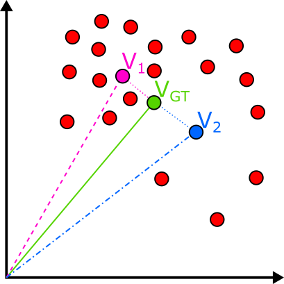
Figure 1: Example of two different predictions for ground truth vector $V_{GT}$, where predicted vector $V_{1}$ has better MSE and COS scores than $V_{2}$, and $V_{2}$ has better RNK score than $V_{1}$. The rest of the points represent vectors of other test samples.

Compared to other solutions, our systems have average or below-average performance in terms of MSE and COS test scores. However, they perform significantly better than the other approaches in terms of RNK test scores, from which we conclude that our solutions are better suited for the retrieval task. This is an interesting situation which we elaborate with the following example, shown in Figure 1. It depicts two different predictions, $V_{1}$ and $V_{2}$, the first with better MSE and COS scores, and the second with a better RNK score. The second solution prefers a vector subspace with a lower density of test samples even if the absolute distance from the correct vector is greater. With a smaller set of possible surrounding solutions, retrieving the vector $V_{GT}$ from the vector $V_{2}$ is more precise than retrieving it from the vector $V_{1}$.

6 Conclusion

Definition Modeling and Reverse Dictionary are two opposite learning tasks for exploring the relationship between different semantic representations of words. CODWOE SemEval task Mickus et al. (2022) is designed to investigate these tasks on five different languages using three different types of word embeddings.

We propose an adaptation of an existing DEFMOD model and analyze its performance and the glosses generated by the model. We believe that DEFMOD is a theoretically interesting problem and that further investigations should focus on discovering which types of semantic generalization the models are able to perform, and how this generalization ability is influenced by both the data and the models’ structure. The existing DEFMOD experiments are largely incomparable since they are based on different data and setups. We believe that a contribution of the CODWOE task is the creation of a multilingual evaluation setting, as well as the use of the flexible MoverScore as an evaluation metric.

Our REVDICT systems are based on deep regression models based on transformer architecture that achieved top scores for the difficult-to-predict sgns (word2vec) embeddings. In most cases our REVDICT solutions perform significantly better then the other systems in terms of the RNK score. These results imply that our solutions could be the appropriate approach for retrieving the right word from its description, a problem crucial for solving the TOT problem Brown and McNeill (1966) in machine-assisted text synthesis.

In summary, the models that we produced for the CODWOE task perform competitively when compared to other participants’ models, and can therefore serve as a reasonable starting point for future tackling of DEFMOD and REVDICT problems. We believe that the promising directions for future optimizations include the construction of multilingual and multi-task models, as well as investigations of the influence of the external data, primarily in the form of huge pre-training corpora.

Appendix A Appendix - Analysis of DEFMOD Data and Models

A.1 Train and Test Data

Motivated by the weak performance of DEFMOD models (see Section 5), we examined whether the distributions of train and test data are comparable. To this end we created 2D projections of sgns and electra embedding for all five languages using the t-SNE method Van der Maaten and Hinton (2008).

The projections, depicted in Figure 2, show that the train and test distributions of the embeddings match well. It is therefore reasonable to expect that the distributions of the gloss texts are similar as well, as the gloss semantics expectedly matches the semantics of the corresponding words. However, this conjecture should be confirmed experimentally, for example by per-gloss aggregation of pretrained word embeddings extracted from huge corpora.

Figure also shows that the electra vectors are more separable than the sgns vectors. The separability of the embedding vectors varies across languages, probably influenced by the corpora used for pre-training of the embeddings. We note that the observations about the train and test embedding distributions are also applicable to the REVDICT problem aimed at the prediction of the embeddings from gloss texts.

Basic gloss statistics can be found in Table 5. There exists a large variation in gloss size between languages, e.g., the longest gloss from the ES dataset is almost twice the size of the longest EN gloss. In addition, the longest glosses in the validation (development) datasets are significantly smaller then those in the train datasets, on average $42.55\%$ smaller. The ’dictionary size’ column in the table is the number of distinct tokens in each dataset. Dictionary sizes vary, for example, EN dictionary is approximately half the size of the RU dictionary. Differences between the gloss and dictionary sizes suggest that it is reasonable to use a separate model for each language.

Basic statistics of the transformed dataset can be found in Table 6. As expected, the transformed glosses are significantly smaller then the glosses in the original dataset. For example, the median transformed gloss size is on average $29.25\%$ smaller.

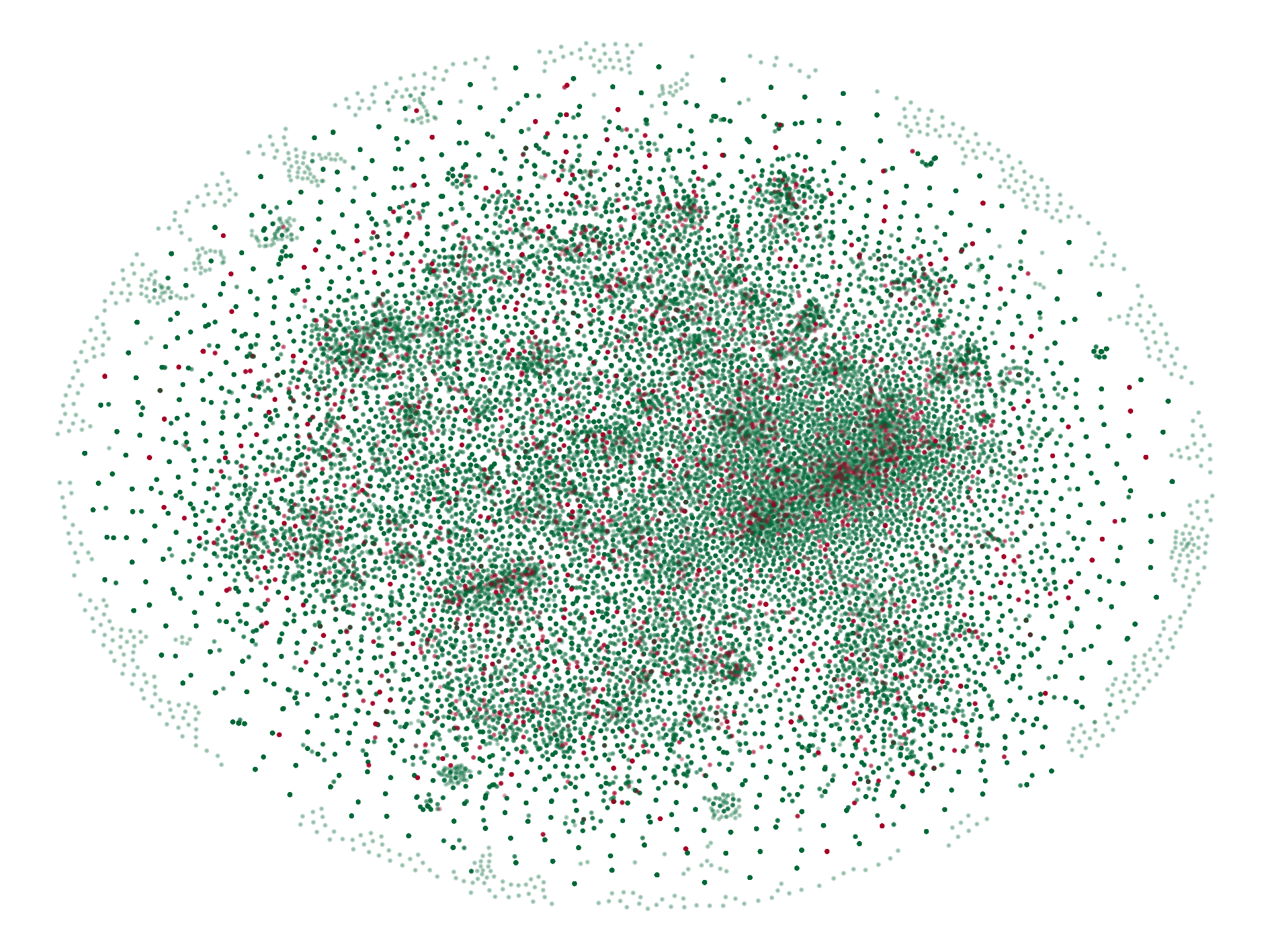
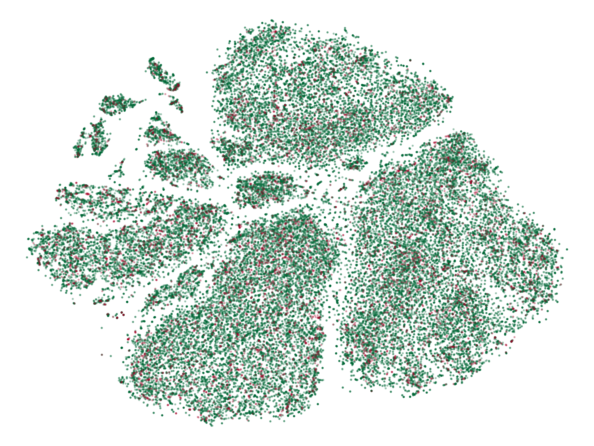
Figure 2: t-SNE projections of the sgns and electra vectors from the train (green) and test (red) datasets. Color intensity is proportional to data density.

EN-SGNS	EN-ELECTRA
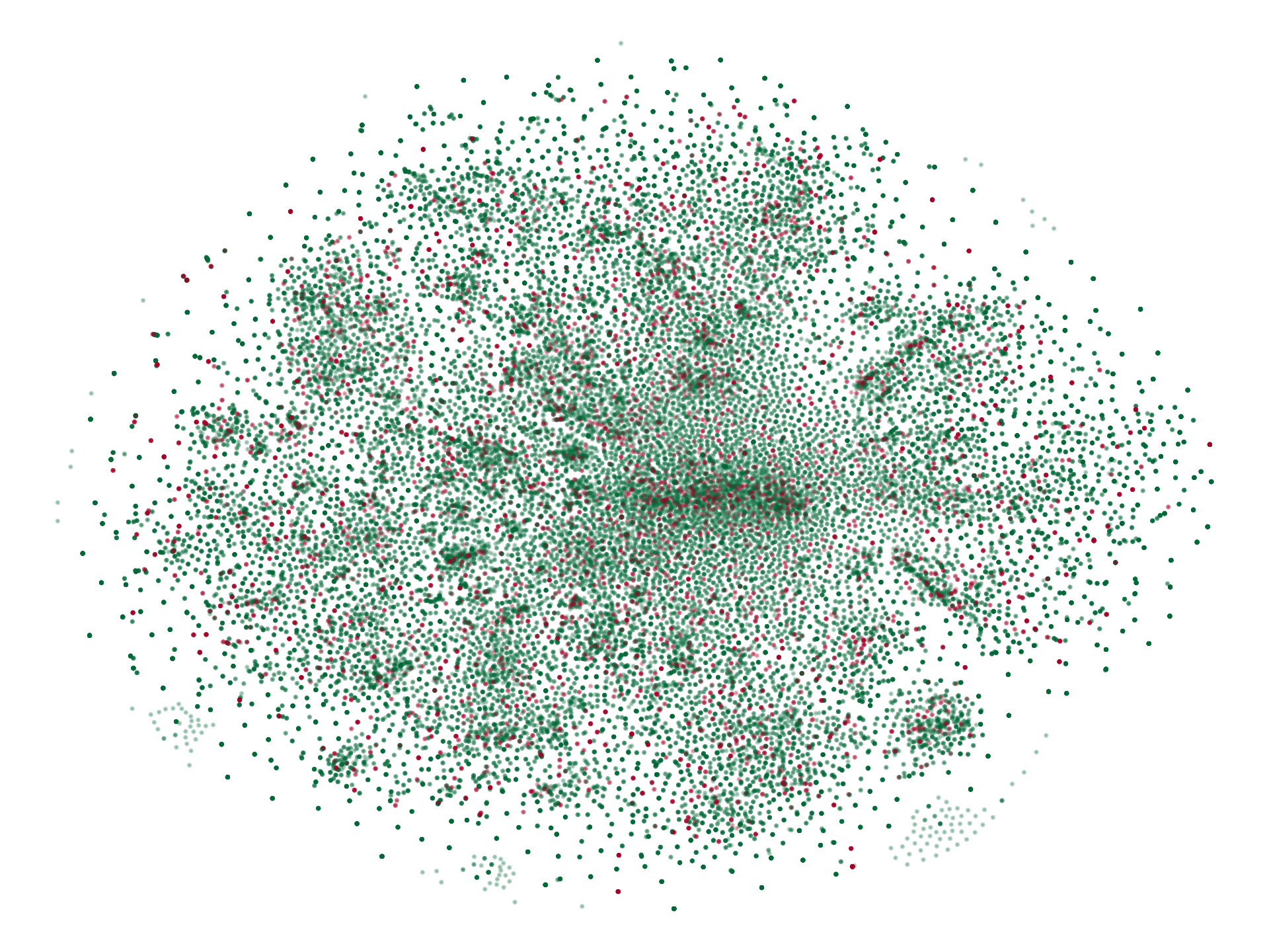
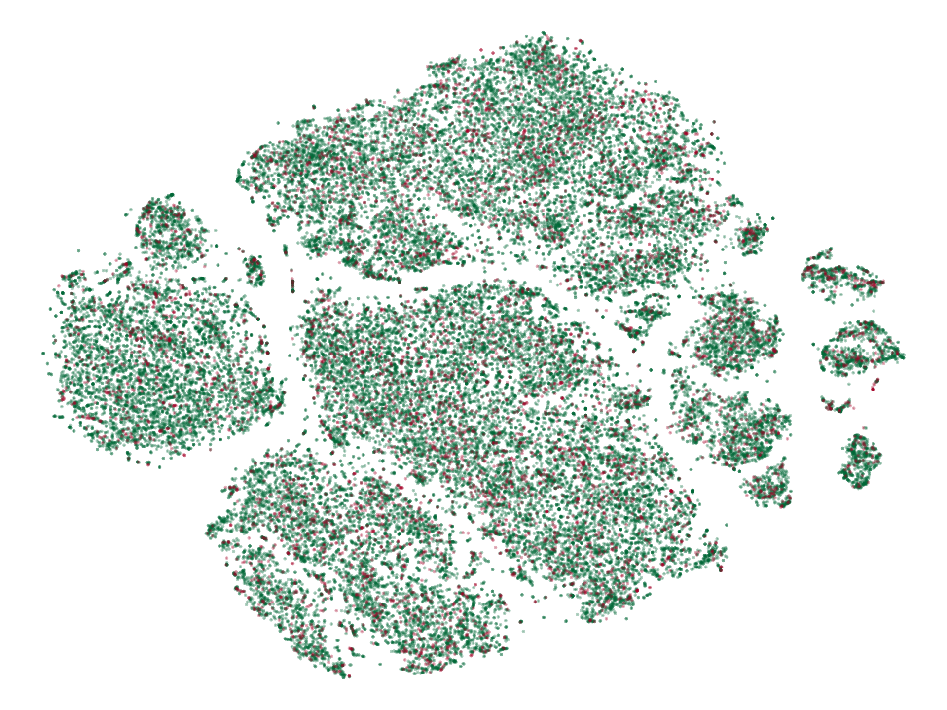
FR-SGNS	FR-ELECTRA
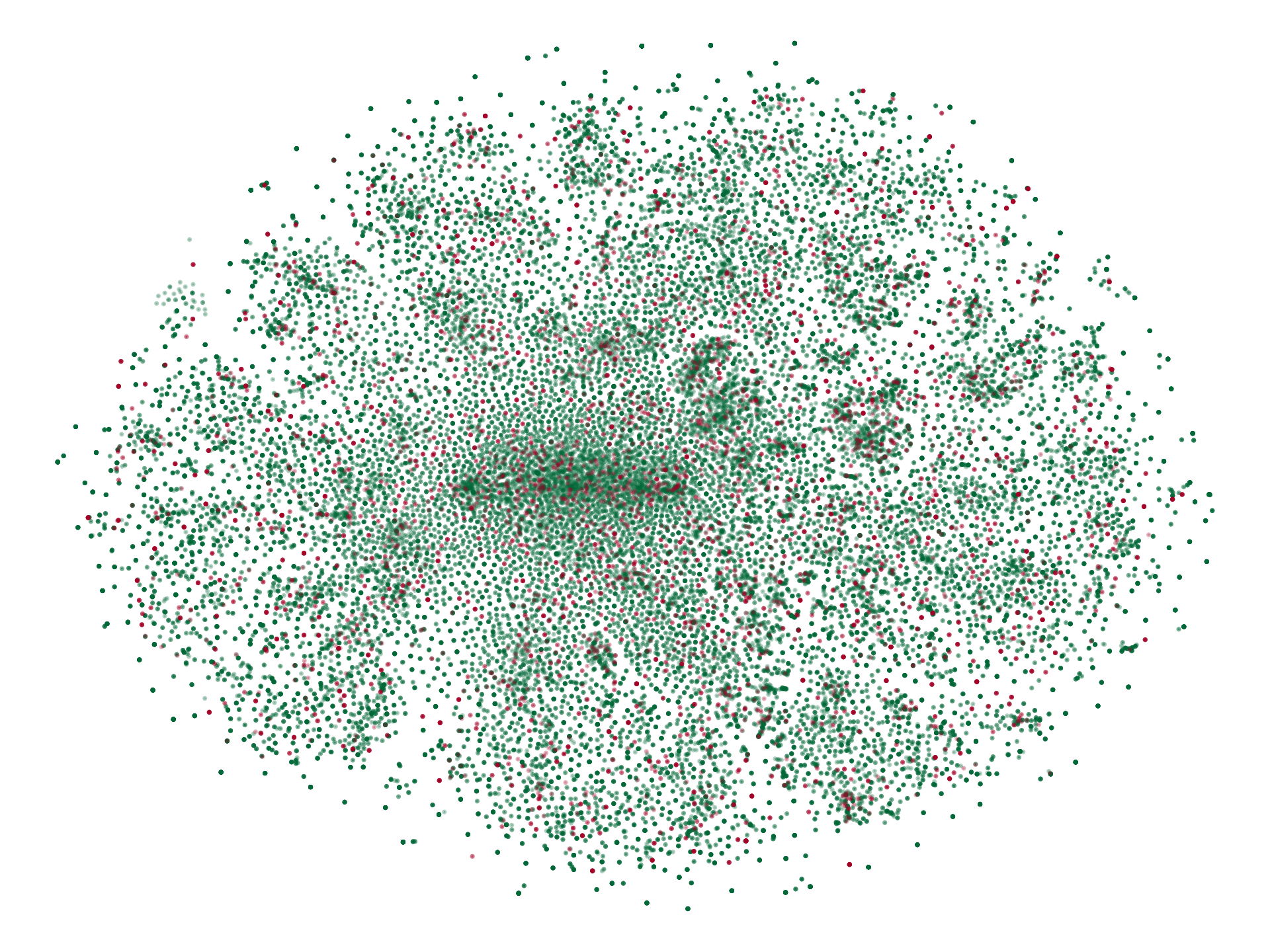
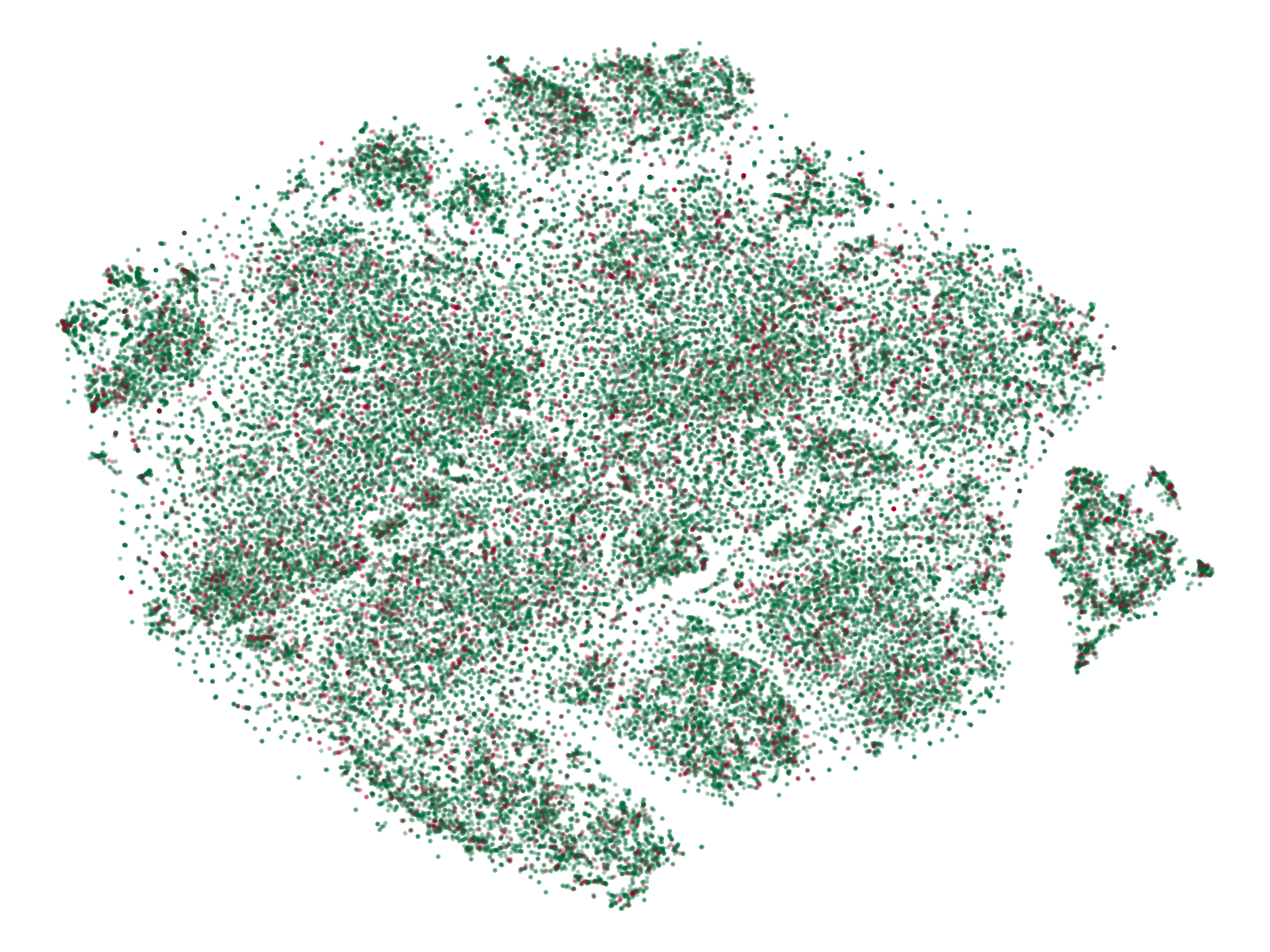
RU-SGNS	RU-ELECTRA
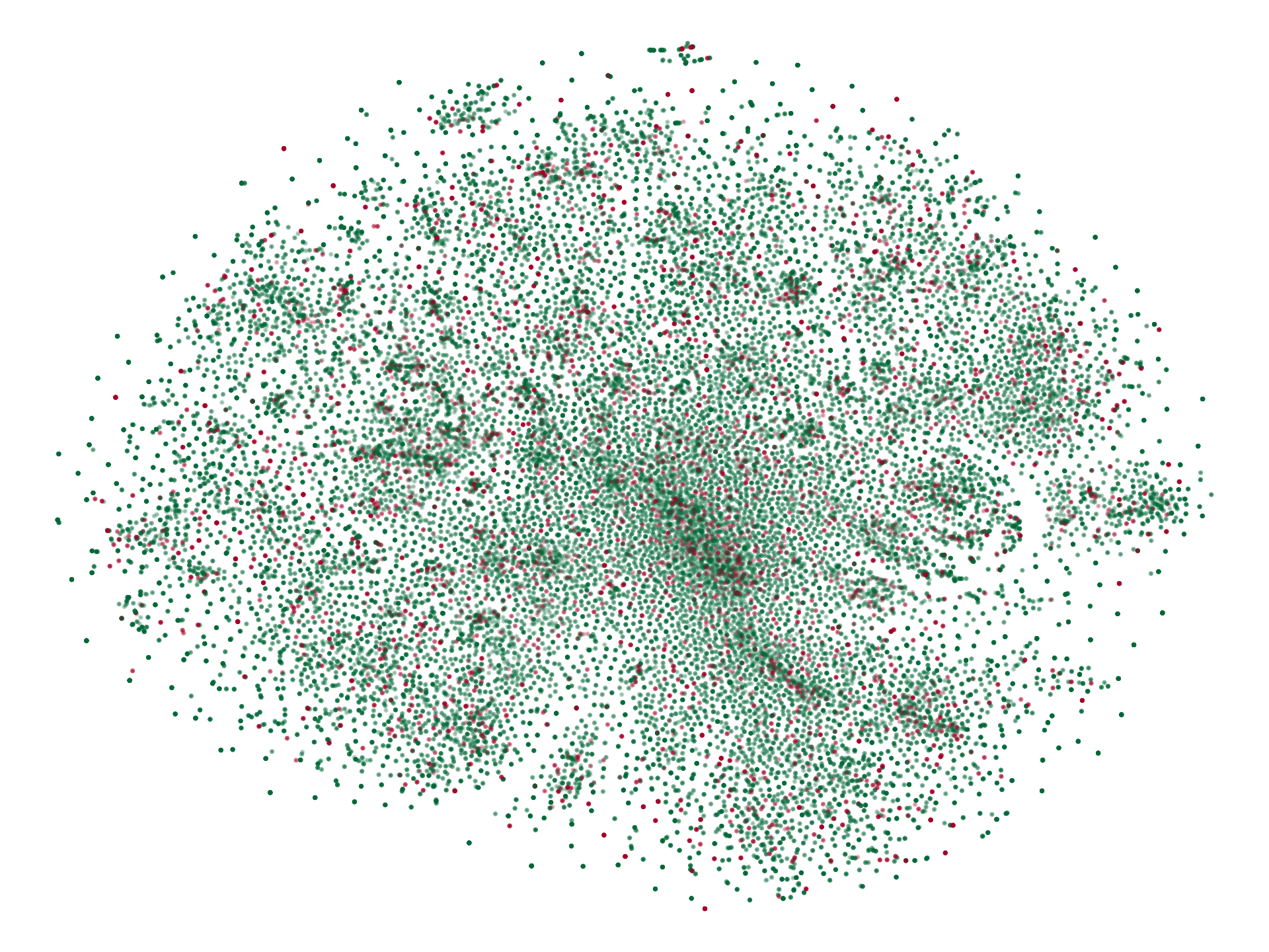
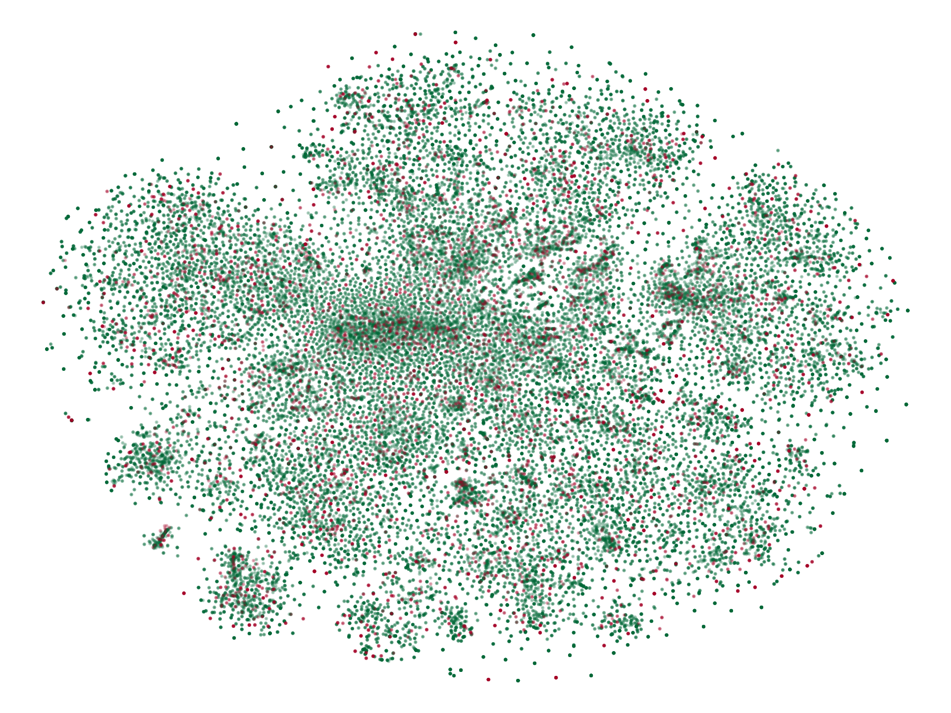
ES-SGNS	IT-SGNS

Lang.	Split	Dict. size	#Tokens	#Glosses	Gloss size
					mean	st.dev	min	q25	median	q75	max
EN	train	29.046	511.531	43.608	11.73	7.98	1	6.0	10.0	15.0	129
EN	dev	9.478	76.073	6.375	11.93	7.98	1	6.0	10.0	15.0	70
ES	train	46.765	647.093	43.608	14.84	13.07	1	7.0	11.0	18.0	257
ES	dev	15.464	91.943	6.375	14.42	12.22	1	7.0	11.0	17.0	159
FR	train	40.032	623.978	43.608	14.31	9.74	1	8.0	12.0	18.0	159
FR	dev	12.760	91.475	6.375	14.35	9.91	1	8.0	12.0	18.0	113
IT	train	40.130	592.409	43.608	13.58	11.01	1	6.0	11.0	18.0	202
IT	dev	14.069	87.531	6.375	13.73	11.61	1	6.0	11.0	18.0	130
RU	train	57.141	492.978	43.608	11.30	7.78	1	6.0	9.0	14.0	169
RU	dev	15.498	70.392	6.375	11.04	7.22	1	6.0	9.0	14.0	74

Table 5: Statistics of the gloss and dictionary sizes for the original train and validation (development) datasets. Sizes are calculated by counting the number of whitespace-delimited tokens.

Lang.	Split	Dict. size	#Tokens	#Glosses	Gloss size
					mean	st.dev	min	q25	median	q75	max
EN	train	25.921	456.673	58.792	7.77	6.97	1	3.0	6.0	10.0	128
EN	dev	8.892	68.145	8.403	8.11	7.06	1	3.0	6.0	11.0	69
ES	train	40.024	595.879	44.543	13.38	12.01	1	6.0	10.0	16.0	168
ES	dev	13.723	84.303	6.493	12.98	11.32	1	6.0	10.0	16.0	158
FR	train	33.963	487.013	46.537	10.47	9.18	1	4.0	8.0	14.0	155
FR	dev	11.216	71.021	6.786	10.47	9.22	1	4.0	8.0	14.0	101
IT	train	39.124	452.028	45.080	10.03	9.03	1	4.0	7.0	13.0	195
IT	dev	13.805	67.211	6.621	10.15	9.40	1	4.0	7.0	13.0	109
RU	train	56.467	428.787	50.843	8.43	6.99	1	4.0	7.0	11.0	142
RU	dev	15.241	61.074	7.509	8.13	6.44	1	4.0	6.0	11.0	72

Table 6: Statistics of the gloss and dictionary sizes for the transformed train and validation (development) datasets. Sizes are calculated by counting the number of whitespace-delimited tokens.

A.2 DEFMOD Models’ Performance

Here we append Section 5 with a more fine-grained analysis of the DEFMOD models. Table 8 contains the models’ performances. As can be seen, the largest gains are achieved by using all of the embedding vectors as input for gloss generation (context=allvec). There exists a negligible difference between the LSTM and GRU RNNs, with GRU performing slightly better. Using a fallback model always slightly improves the MoverScore of a model. In Table 8 the architecture of the fallback model is the architecture of the main model with the corresponding parameter replaced with the value in the ’fallback’ column. Interestingly, using contextual electra vectors does not help, i.e., the sgns (word2vec) vectors which are not context-aware perform comparably. This is true even when only a single embedding is used, i.e., when context equals electra. The equality of sgns and electra is unexpected since both the train and test datasets contain polysemous electra vectors and words with multiple senses.

It is also interesting to consider the influence of the training data on the model’s performance. We hypothesize that a DEFMOD model’s score on a single test example is positively correlated with the semantic closeness of the example to the examples in the train set. To test this hypothesis we calculate Spearman correlation between test MoverScore and BLEU on one, and the cosine similarity of the test embedding and most similar train embeddings. This is done for the best-performing submitted model from Table 8. We also calculate the average scores on two sets of $10\%$ test examples that are least similar and most similar to the train examples. Since the embeddings (sgns and electra) were built on large outside corpora, it is reasonable to believe that they capture semantic similarity of the associated words and glosses. Surprisingly, the results show a lack of consistent and strong correlation and the correlations range from weakly negative to weakly positive, depending on both the language and the embedding type. This lack of correlation could be caused by many factors, including the nature of the model, the nature of the pretrained embeddings, and the semantics of the cosine similarity measure.

The future extensions and improvements of the proposed analysis could reveal the nature of the train data necessary for the DEFMOD models to successfully generalize, and perhaps point to a similarity measure that reveals more fine-grained properties of such a generalization.

Table 7: Correlation between the best DEFMOD model’s scores on one, and the closeness of the test examples to the train set on the other side. The unit of correlation is an example from the test set, and its similarity to the train set is calculated as the average cosine similarity with the $10$ most similar train embeddings. The last two columns contain average model scores on $10\%$ of the least and most train-similar test examples.

	Correlation of Score and Similarity				Avg. Score for Similarity Percentile
	MVR		BLEU		MVR		BLEU
LANG-EMB	spearman $\rho$	p-value	spearman $\rho$	p-value	bottom 10%	top 10%	bottom 10%	top 10%
EN-SGNS	0.0458	0.0003	0.0019	0.8831	0.0852	0.1004	0.0328	0.0297
EN-ELKT	0.0096	0.4508	0.0186	0.1414	0.0889	0.1182	0.0293	0.0503
FR-SGNS	-0.0625	0.0000	-0.1270	0.0000	0.0801	0.0427	0.0363	0.0222
FR-ELKT	0.0433	0.0006	0.0838	0.0000	0.0387	0.0760	0.0214	0.0322
RU-SGNS	0.0758	0.0000	0.0353	0.0054	0.0754	0.0947	0.0310	0.0279
RU-ELKT	0.0000	0.9979	-0.0063	0.6217	0.0748	0.0677	0.0279	0.0244
ES-SGNS	0.0458	0.0003	0.0019	0.8831	0.1084	0.1052	0.0523	0.0552
IT-SGNS	-0.0528	0.0000	0.0047	0.7084	0.1082	0.0783	0.0111	0.0128

Table 8: Performance of best DEFMOD models. Overall best models from all the participants are included for comparison. Submitted models are colored gray and the best submitted results are bolded. The best overall results are colored red. Other models are included to illustrate the influence of design choices.

MODEL PARAMS					EN			ES			FR			IT			RU
context	seed	rnn	fallback	#epochs	MVR	BLEU	lBLEU	MVR	BLEU	lBLEU	MVR	BLEU	lBLEU	MVR	BLEU	lBLEU	MVR	BLEU	lBLEU
BEST					0.135	0.033	0.043	0.128	0.045	0.064	0.075	0.029	0.038	0.117	0.066	0.099	0.148	0.049	0.072
sgns	sgns	gru		$300$	0.070	0.027	0.034	0.083	0.039	0.058	0.039	0.024	0.028	0.073	0.009	0.014	0.073	0.023	0.031
allvec	sgns	gru		$300$	0.085	0.031	0.040	0.092	0.045	0.064	0.048	0.026	0.032	0.072	0.009	0.014	0.077	0.027	0.035
allvec	sgns	gru	sgns	$300$	0.089	0.032	0.040	0.093	0.045	0.064	0.055	0.026	0.031	0.074	0.009	0.014	0.080	0.027	0.035
sgns	sgns	gru		$450$	0.077	0.029	0.038	0.080	0.037	0.057	0.048	0.026	0.031	0.071	0.009	0.014	0.073	0.022	0.029
sgns	sgns	lstm		$450$	0.075	0.028	0.035	0.082	0.038	0.056	0.052	0.025	0.030	0.070	0.015	0.009	0.073	0.022	0.030
allvec	sgns	gru		$450$	0.093	0.033	0.042	0.089	0.044	0.062	0.049	0.028	0.033	0.076	0.010	0.015	0.075	0.027	0.036
allvec	sgns	lstm		$450$	0.091	0.033	0.041	0.092	0.044	0.061	0.051	0.027	0.032	0.076	0.010	0.015	0.076	0.026	0.033
allvec	sgns	gru	sgns	$450$	0.096	0.033	0.042	0.096	0.044	0.063	0.061	0.028	0.033	0.077	0.010	0.015	0.082	0.028	0.037
allvec	sgns	lstm	sgns	$450$	0.095	0.033	0.042	0.093	0.044	0.061	0.057	0.027	0.032	0.077	0.010	0.015	0.079	0.026	0.034
allvec	sgns	lstm	gru	$450$	0.094	0.033	0.042	0.092	0.044	0.061	0.056	0.027	0.032	0.077	0.010	0.015	0.078	0.026	0.033
electra	electra	gru		$450$	0.079	0.028	0.034				0.050	0.029	0.024				0.072	0.024	0.031
allvec	electra	gru		$450$	0.091	0.032	0.041				0.047	0.027	0.032				0.073	0.027	0.035
electra	electra	gru	sgns	$450$	0.094	0.033	0.041				0.058	0.026	0.031				0.082	0.028	0.036

A.3 Qualitative Analysis of Generated Glosses

The DEFMOD models achieve weak results in comparison to the previous state-of-art approaches, which is probably due to the comparably small amount of training and pretraining data. Here we demonstrate that the generated glosses can nevertheless capture a degree of the semantics of the correct glosses.

Table 9 shows four categories of semantic similarity between the correct and model-generated glosses, in descending order (highest similarity first). These categories include hits or near hits (correct glosses), “near misses” (glosses that capture a significant amount of the original meaning), somewhat similar glosses, and complete misses. Several examples demonstrate that the subword-based models can produce syntactically incorrect glosses.

Table 10 contains generated glosses for different senses of the word “consider”, which demonstrate that the model was able to approximate, to a degree, the semantics of the senses.

A principled analysis of the generated and correct glosses, based on a well defined semantic annotation scheme, might prove revealing but it would be time-consuming and impractical. Therefore it would be of interest to automatize such efforts. It would be interesting to explore if this can be done using large pretrained transformers able to measure fine-grained semantic similarity.

Table 9: Glosses generated by the top submitted DEFMOD model, alongside the correct glosses. The examples are ordered by descending semantic similarity between the correct and the generated gloss.

Word	True Gloss / Generated Gloss
lamebrain	A fool
	A fool , idiot
sentiment	A general thought , feeling , or sense
	A feeling or feeling of thinking
available	Such as one may avail oneself of ; capable of being used for the accomplishment of a purpose
	Able to be used
model	A representation of a physical object , usually in miniature
	An act of designing
supernumerary	Of an organ or structure : additional to what is normally present
	Having four wings
navy	Belonging to the navy ; typical of the navy
	To be armed
fuzzy	Vague or imprecise
	lacking
co-opt	To absorb or assimilate into an established group
	To conceal
misinformation	Information that is incorrect
	prejudice
cutthroat	Ruthlessly competitive , dog-eat-dog
	Very large
discretional	discretionary
	Of or pertaining to
abundantly	In an abundant manner ; in a sufficient degree ; in large measure
	In a very manner

Glosses generated by the top submitted DEFMOD model, alongside the correct glosses, for the multiple senses of the word “consider”. Word True Gloss (describing the sense) / Generated Gloss consider To assign some quality to To hold the opinion consider To look at attentively To make something certain consider To have regard to ; to take into view or account ; to pay due attention to ; to respect To hold into consider To think of doing To permit consider To debate ( or dispose of ) a motion To make something certain

Table 10:

Appendix B Appendix - Analysis of REVDICT Data and Models

B.1 Data Analysis

Here we analyze the properties of the pretrained embedding vectors assigned to the words defined by the glosses. We start by analyzing the numeric values contained in the vectors. Basic statistics of vector elements can be found in Table 11. It is noticeable that there are large variations in value depending on the language and the embedding type. For example, there is a significant difference between maximum values, especially between electra and sgns. To further investigate the vector elements, we visualize the shapes of their distributions for train datasets (Figure 3 and 4). Distribution shapes look similar for dev datasets.

Next, we explore the vector data by reducing dimensionality to the 2D space using the Pairwise Controlled Manifold Approximation Projection (PaCMAP) algorithm Wang et al. (2020). Figure 5 shows the distributions of all three types of embeddings in the train and validation (development) datasets for English, French, and Russian. We also visualize distributions of sgns (word2vec) and char embeddings for all languages, in Figure 6. As can be seen, the vector distributions vary greatly between the embedding types. Additionally, for all the embedding types, the vectors of different languages occupy a distinct area and are easily separable.

We further investigate the relationships between different embeddings in the following way. We first cluster the values of the electra vectors with k-means algorithm. We set the number of clusters to five and assign a different color to each cluster. We retain the electra cluster-based color of the samples (glosses) while visualizing the vectors of other embedding types, as shown in Figure 7. It can be clearly seen that the electra-based clusters are not preserved for other embedding types.

B.2 Model Performance

Here we present validation and test scores for our six REVDICT solutions described in Section 4.2. We use the following metrics for internal validation of our REVDICT solutions: Mean Squared Error (MSE), Cosine Similarity (COS) and Central Kernel Alignment (CKA) Kornblith et al. (2019); Cortes et al. (2012). Validation scores for each REVDICT approach can be found in Table 12. The last three rows contain the total scores for each metric and each of our REVDICT solutions. A total score is the sum of the values of all datasets and we use it for a simple comparison of solutions. It is evident that each subsequent approach gives better validation results than the previous ones.

Test predictions are scored by these metrics: MSE, COS, and Cosine-Based Ranking (RNK). The RNK measure is defined as the proportion of test samples with cosine similarity to the model output embedding higher than the ground truth embedding. The final results for all our solutions can be found in Table 13. Here, each subsequent approach has lower scores than the previous ones, which is the complete opposite of the validation results. This suggests potential overfitting to the dev dataset that could be the result of Bayesian hyperparameter optimization (BHO). However, this is contrary to expectations as the last two solutions have three times fewer BHO points and should not overfit to the dev dataset. The reason for this phenomenon is unclear and needs further investigation.

The best REVDICT results for each team can be found in Table 14 for MSE score, Table 15 for COS score, and Table 16 for RNK score. When compared to other solutions, our systems have low to average performance according to the MSE scores. For the COS scores, our systems have very good performance on sgns (word2vec) vectors, and low performance on other embedding types. In terms of the RNK (ranking) our systems almost always yield the top performance, and this result is consistent across languages and embedding types.

lang	split	vector	min	mean	max	abs-min	abs-mean	abs-max
en	train	sgns	-8.66	0.012	8.33	2.40-08	0.641	8.66
en	train	char	-5.48	0.081	31.10	6.60-09	0.341	31.10
en	train	electra	-126.26	0.033	85.62	1.00-10	0.598	126.26
en	dev	sgns	-7.02	0.013	7.30	9.51-08	0.657	7.30
en	dev	char	-5.48	0.083	7.31	8.75-08	0.341	7.31
en	dev	electra	-48.24	0.028	52.19	1.00-09	0.587	52.19
it	train	sgns	-9.41	-0.014	9.72	6.60-09	0.700	9.72
it	train	char	-13.37	0.013	20.02	1.62-07	0.553	20.02
it	dev	sgns	-8.22	-0.013	7.82	1.02-07	0.706	8.22
it	dev	char	-9.95	0.008	16.23	3.96-07	0.551	16.23
fr	train	sgns	-10.38	-0.013	9.39	1.59-08	0.682	10.38
fr	train	char	-23.42	0.306	11.07	1.12-08	0.574	23.42
fr	train	electra	-46.24	0.045	89.07	3.00-10	0.644	89.07
fr	dev	sgns	-7.57	-0.017	7.81	3.51-07	0.666	7.81
fr	dev	char	-14.60	0.307	7.80	2.62-07	0.574	14.60
fr	dev	electra	-42.73	0.045	51.29	9.00-10	0.655	51.29
es	train	sgns	-9.79	-0.018	9.72	2.15-08	0.653	9.79
es	train	char	-15.03	0.577	13.37	2.27-07	0.822	15.03
es	dev	sgns	-9.32	-0.021	7.22	8.86-08	0.658	9.32
es	dev	char	-13.19	0.577	11.40	2.28-06	0.820	13.19
ru	train	sgns	-7.82	0.002	8.08	1.17-07	0.446	8.08
ru	train	char	-16.87	0.139	8.04	8.00-10	0.311	16.87
ru	train	electra	-30.24	-0.017	22.56	1.75-08	0.788	30.24
ru	dev	sgns	-8.06	0.002	7.91	7.94-08	0.439	8.06
ru	dev	char	-11.86	0.140	8.01	3.05-07	0.310	11.86
ru	dev	electra	-22.53	-0.017	21.70	4.75-08	0.789	22.53

Table 11: Statistics of the elements of the embedding vectors from the train and validation (development) datasets.

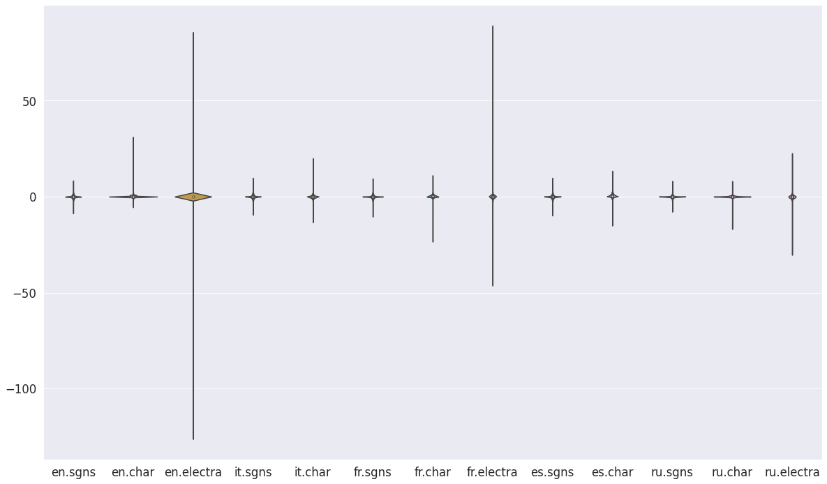
Figure 3: Distributions of vector elements in train datasets.

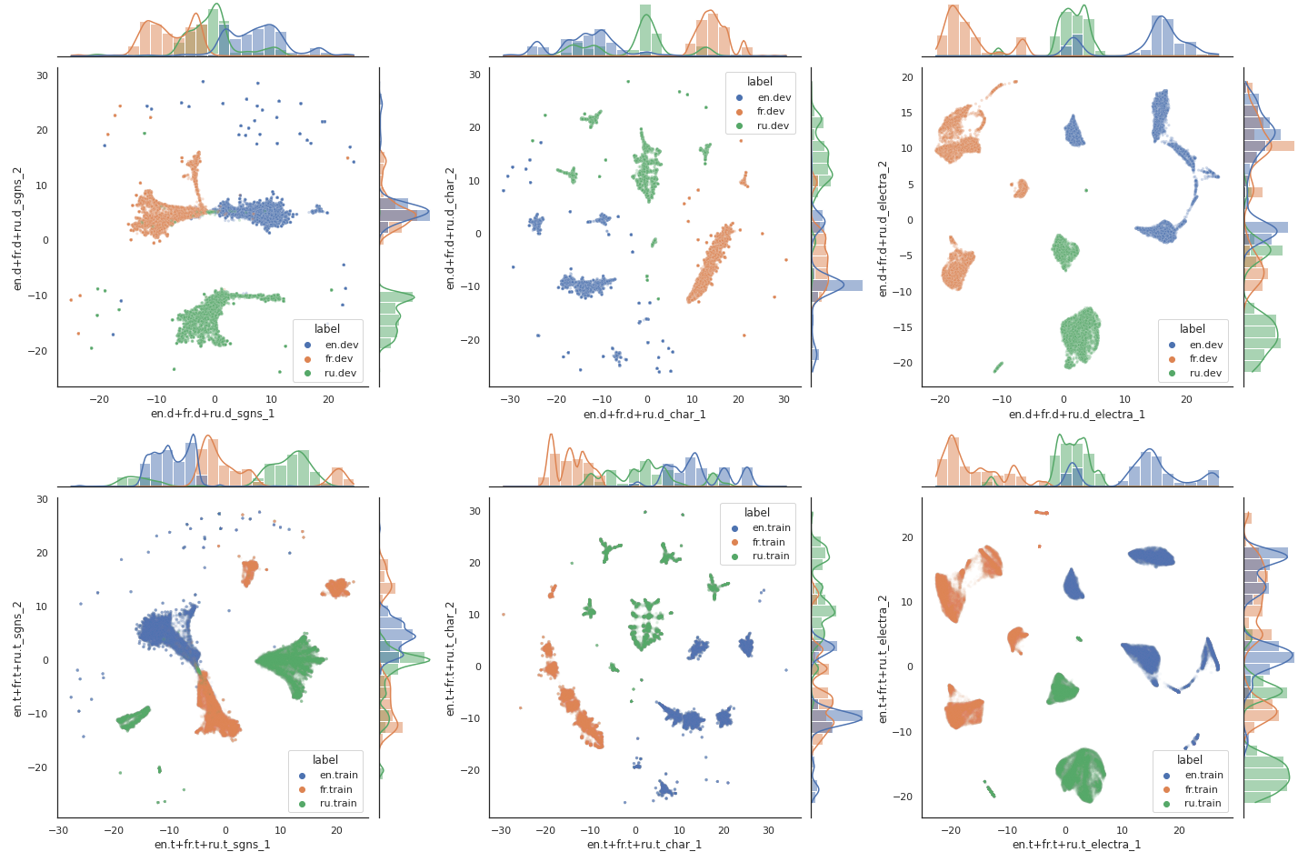
Figure 5: Distributions of all three embedding types in train (2nd row) and validation (development, 1st row) datasets after dimensionality reduction to 2D space. sgns (word2vec, 1st column), char (2nd column), and electra (3rd column) embeddings are depicted for English (orange), French (green), and Russian (blue).

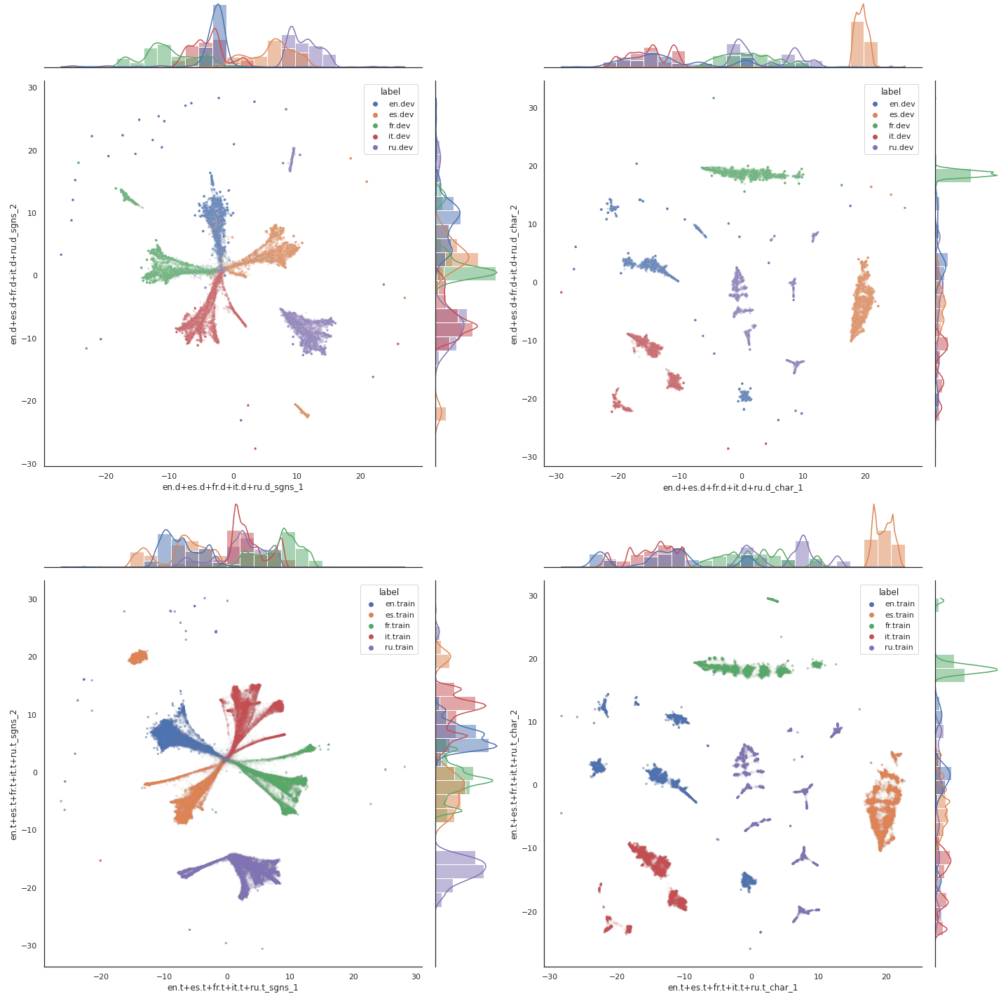
Figure 6: Distributions of sgns (1st column) and char (2nd column) embeddings in train (2nd row) and validation (development, 1st row) datasets after dimensionality reduction to 2D space. The embeddings are depicted for English (blue), Spanish (orange), French (green), Italian (red), and Russian (violet).

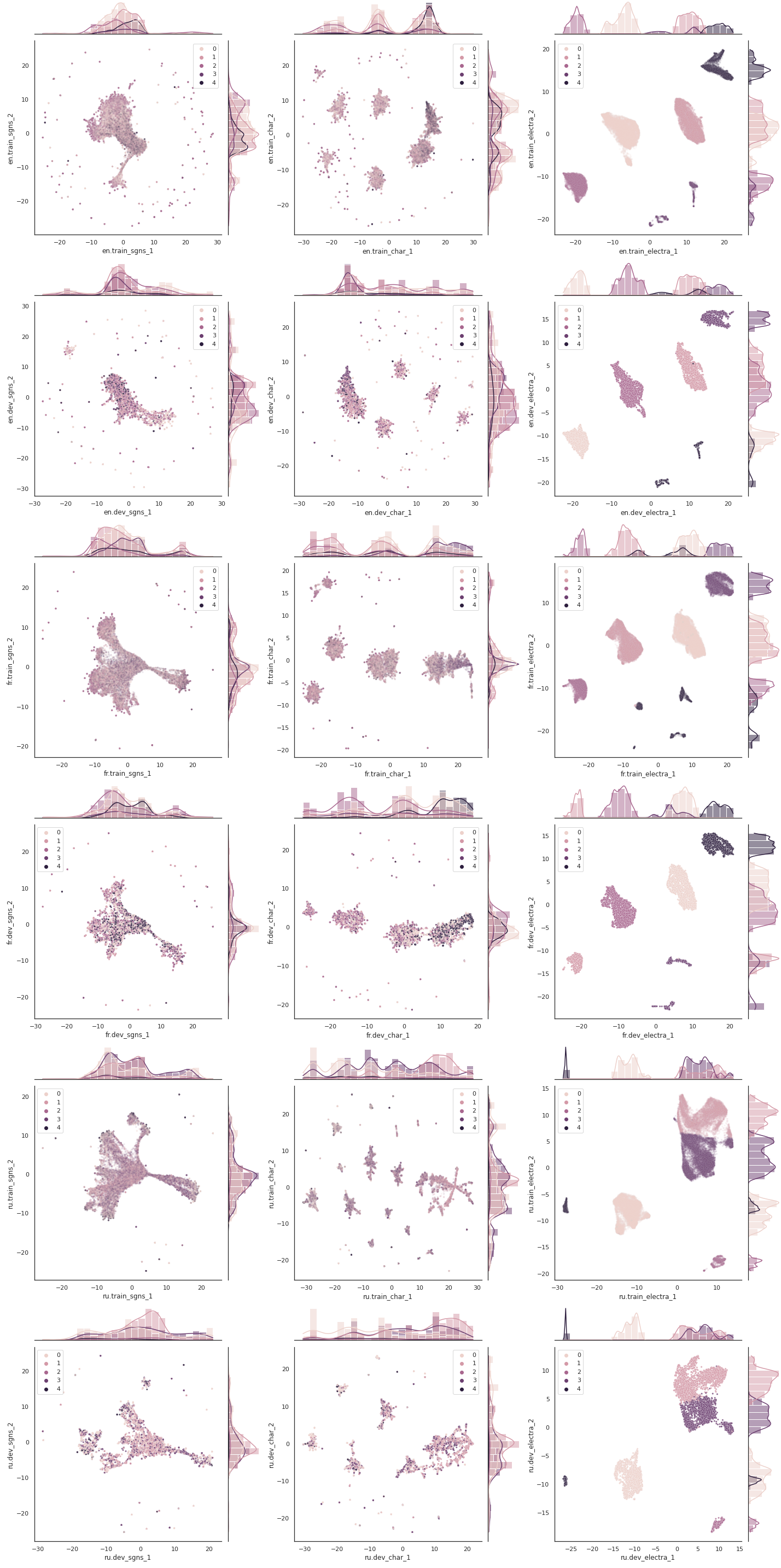
Figure 7: Projection of the clusters in the electra embedding space (3rd column) to the spaces of the other two embedding types sgns (1st column) and char (2nd column). The analysis if performed for English (rows 1–2), French (rows 3–4), and Russian (rows 5–6) train and validation (development) datasets, after dimensionality reduction to 2D space.

METRICS	RD 1	RD 2	RD 3	RD 4	RD 5	RD 6	BEST
mse-en-sgns	0.521	0.632	0.521	0.428	0.348	0.343	0.343
mse-en-char	0.088	0.091	0.051	0.098	0.058	0.090	0.051
mse-en-electra	0.611	0.683	0.612	0.560	0.439	0.295	0.295
mse-it-sgns	0.846	0.700	0.783	0.650	0.670	0.485	0.485
mse-it-char	0.264	0.235	0.253	0.258	0.224	0.222	0.222
mse-fr-sgns	0.773	0.671	0.629	0.585	0.514	0.443	0.443
mse-fr-char	0.210	0.205	0.211	0.246	0.180	0.178	0.178
mse-fr-electra	0.634	0.616	0.518	0.651	0.400	0.360	0.360
mse-es-sgns	0.627	0.764	0.675	0.560	0.543	0.562	0.543
mse-es-char	0.341	0.338	0.323	0.353	0.291	0.265	0.265
mse-ru-sgns	0.363	0.236	0.268	0.207	0.162	0.109	0.109
mse-ru-char	0.053	0.060	0.062	0.060	0.038	0.051	0.038
mse-ru-electra	0.544	0.481	0.519	0.497	0.313	0.421	0.313
cos-en-sgns	0.483	0.453	0.492	0.537	0.571	0.549	0.571
cos-en-char	0.875	0.871	0.927	0.860	0.918	0.873	0.927
cos-en-electra	0.895	0.887	0.896	0.900	0.915	0.938	0.938
cos-it-sgns	0.470	0.510	0.482	0.527	0.521	0.580	0.580
cos-it-char	0.801	0.824	0.810	0.807	0.834	0.836	0.836
cos-fr-sgns	0.457	0.490	0.508	0.522	0.544	0.556	0.556
cos-fr-char	0.866	0.870	0.866	0.843	0.886	0.887	0.887
cos-fr-electra	0.894	0.894	0.904	0.892	0.921	0.929	0.929
cos-es-sgns	0.501	0.450	0.486	0.531	0.539	0.538	0.539
cos-es-char	0.881	0.883	0.887	0.878	0.899	0.908	0.908
cos-ru-sgns	0.525	0.599	0.582	0.618	0.662	0.674	0.674
cos-ru-char	0.933	0.925	0.922	0.925	0.952	0.935	0.952
cos-ru-electra	0.807	0.821	0.811	0.817	0.872	0.841	0.872
cka-en-sgns	0.755	0.776	0.879	0.939	0.889	0.895	0.939
cka-en-char	0.991	0.994	0.998	0.996	0.996	0.994	0.998
cka-en-electra	0.993	0.995	0.997	0.998	0.997	0.998	0.998
cka-it-sgns	0.608	0.773	0.811	0.905	0.780	0.857	0.905
cka-it-char	0.979	0.989	0.992	0.993	0.989	0.990	0.993
cka-fr-sgns	0.647	0.779	0.860	0.916	0.838	0.866	0.916
cka-fr-char	0.981	0.989	0.993	0.991	0.990	0.991	0.993
cka-fr-electra	0.991	0.995	0.997	0.996	0.997	0.997	0.997
cka-es-sgns	0.685	0.698	0.826	0.909	0.802	0.795	0.909
cka-es-char	0.982	0.989	0.993	0.992	0.991	0.992	0.993
cka-ru-sgns	0.611	0.821	0.850	0.927	0.880	0.927	0.927
cka-ru-char	0.995	0.997	0.998	0.998	0.997	0.997	0.998
cka-ru-electra	0.978	0.989	0.992	0.994	0.994	0.991	0.994
TOTAL mse	5.875	5.712	5.425	5.153	4.180	3.824	3.824
TOTAL cos	9.388	9.477	9.573	9.657	10.034	10.044	10.044
TOTAL cka	11.196	11.784	12.186	12.554	12.140	12.290	12.554

Table 12: Validation scores for all our REVDICT (RD) approaches. For each score, comparative results are shown in color. Green is used for the best and red for the worst-performing solution per row (a metric defines whether higher or lower values are better). The total score is the sum of the values over all datasets and embeddings.

METRICS	RD 1	RD 2	RD 3	RD 4	RD 5	RD 6	BEST
mse-en-sgns	1.024	0.964	1.021	1.085	1.170	1.119	0.964
mse-en-char	0.169	0.169	0.186	0.162	0.195	0.172	0.162
mse-en-electra	1.723	1.685	1.690	1.768	1.863	1.988	1.685
mse-it-sgns	1.076	1.160	1.100	1.156	1.211	1.318	1.076
mse-it-char	0.366	0.383	0.376	0.370	0.399	0.399	0.366
mse-fr-sgns	1.068	1.119	1.134	1.147	1.250	1.319	1.068
mse-fr-char	0.409	0.419	0.418	0.390	0.447	0.434	0.390
mse-fr-electra	1.339	1.347	1.414	1.358	1.554	1.566	1.339
mse-es-sgns	0.941	0.883	0.924	0.965	1.031	1.020	0.883
mse-es-char	0.526	0.545	0.546	0.532	0.582	0.635	0.526
mse-ru-sgns	0.568	0.604	0.596	0.601	0.667	0.653	0.568
mse-ru-char	0.145	0.141	0.142	0.140	0.170	0.144	0.140
mse-ru-electra	0.911	0.944	0.956	0.961	1.105	1.049	0.911
cos-en-sgns	0.250	0.260	0.250	0.245	0.231	0.214	0.260
cos-en-char	0.761	0.761	0.743	0.770	0.734	0.765	0.770
cos-en-electra	0.821	0.828	0.824	0.818	0.812	0.792	0.828
cos-it-sgns	0.380	0.358	0.370	0.361	0.361	0.339	0.380
cos-it-char	0.724	0.713	0.717	0.721	0.709	0.711	0.724
cos-fr-sgns	0.342	0.336	0.333	0.330	0.319	0.255	0.342
cos-fr-char	0.744	0.738	0.739	0.756	0.725	0.734	0.756
cos-fr-electra	0.847	0.842	0.837	0.844	0.828	0.825	0.847
cos-es-sgns	0.362	0.367	0.361	0.349	0.350	0.354	0.367
cos-es-char	0.819	0.812	0.812	0.816	0.803	0.784	0.819
cos-ru-sgns	0.412	0.421	0.411	0.406	0.399	0.381	0.421
cos-ru-char	0.818	0.822	0.820	0.824	0.788	0.821	0.824
cos-ru-electra	0.724	0.712	0.715	0.712	0.683	0.702	0.724
rnk-en-sgns	0.247	0.234	0.246	0.231	0.252	0.262	0.231
rnk-en-char	0.438	0.439	0.419	0.448	0.438	0.444	0.419
rnk-en-electra	0.438	0.446	0.437	0.444	0.438	0.432	0.432
rnk-it-sgns	0.165	0.177	0.178	0.169	0.188	0.187	0.165
rnk-it-char	0.397	0.390	0.400	0.402	0.397	0.383	0.383
rnk-fr-sgns	0.214	0.203	0.212	0.193	0.229	0.262	0.193
rnk-fr-char	0.425	0.429	0.427	0.435	0.431	0.421	0.421
rnk-fr-electra	0.447	0.463	0.448	0.450	0.444	0.429	0.429
rnk-es-sgns	0.197	0.214	0.203	0.199	0.217	0.201	0.197
rnk-es-char	0.407	0.409	0.403	0.412	0.407	0.420	0.403
rnk-ru-sgns	0.161	0.153	0.175	0.154	0.166	0.150	0.150
rnk-ru-char	0.361	0.365	0.376	0.372	0.378	0.357	0.357
rnk-ru-electra	0.350	0.355	0.351	0.359	0.351	0.345	0.345
TOTAL mse	10.266	10.363	10.504	10.634	11.645	11.817	10.266
TOTAL cos	8.004	7.971	7.931	7.951	7.742	7.677	8.004
TOTAL rnk	4.248	4.276	4.275	4.268	4.337	4.293	4.248

Table 13: Test results for all our REVDICT (RD) approaches. For each score, comparative results are shown in color. Green is used for the best and red for the worst-performing solution per row (a metric defines whether higher or lower values are better). The total score is the sum of the values over all datasets and embeddings.

TEAM	EN			ES		FR			IT		RU
	sgns	char	electra	sgns	char	sgns	char	electra	sgns	char	sgns	char	electra
0	0.909			0.913		1.122			1.196		0.615
1	0.964	0.162	1.685	0.883	0.526	1.068	0.390	1.339	1.076	0.366	0.568	0.140	0.911
2				0.911
3	0.854
5	0.864	0.143	1.310	0.860	0.467	1.026	0.335	1.066	1.031	0.334	0.538	0.116	0.828
6	0.900	0.143	1.340
7	0.915	0.168		0.906	0.557	1.100	0.391		1.097	0.364	0.578	0.156
10	0.875	0.141	1.301						1.087	0.355
12	0.895	0.143	1.326	0.910	0.510	1.107	0.366	1.112	1.111	0.359	0.566	0.132	0.864
13	0.862	0.176	1.509	0.858	0.583	1.030	0.411	1.271	1.039	0.438	0.528	0.184	0.828

Table 14: MSE test scores for each team in REVDICT task. The results of our team are bold (team 1). For each task, comparative results are shown in color. Green is used for the best and red for the worst-performing solution per column.

TEAM	EN			ES		FR			IT		RU
	sgns	char	electra	sgns	char	sgns	char	electra	sgns	char	sgns	char	electra
0	0.156			0.223		0.216			-0.004		0.006
1	0.260	0.770	0.828	0.367	0.819	0.342	0.756	0.847	0.380	0.724	0.421	0.824	0.724
2				0.403
3	0.248
5	0.241	0.795	0.847	0.347	0.839	0.312	0.789	0.862	0.374	0.747	0.383	0.852	0.735
6	0.185	0.796	0.846
7	0.194	0.792		0.262	0.820	0.228	0.769		0.260	0.739	0.335	0.836
10	0.204	0.798	0.843						0.274	0.734
12	0.166	0.795	0.844	0.252	0.824	0.212	0.770	0.858	0.246	0.728	0.298	0.830	0.721
13	0.243	0.782	0.846	0.353	0.824	0.328	0.752	0.859	0.360	0.681	0.424	0.791	0.734

Table 15: COS test scores for each team in REVDICT task. The results of our team are bold (team 1). For each task, comparative results are shown in color. Green is used for the best and red for the worst-performing solution per column.

TEAM	EN			ES		FR			IT		RU
	sgns	char	electra	sgns	char	sgns	char	electra	sgns	char	sgns	char	electra
0	0.499			0.495		0.498			0.499		0.499
1	0.231	0.419	0.432	0.197	0.403	0.193	0.421	0.429	0.165	0.383	0.150	0.357	0.345
2				0.167
3	0.319
5	0.326	0.500	0.490	0.271	0.424	0.302	0.428	0.476	0.197	0.428	0.247	0.389	0.417
6	0.500	0.500	0.500
7	0.374	0.478		0.375	0.410	0.439	0.416		0.384	0.438	0.291	0.377
10	0.394	0.483	0.478						0.386	0.478
12	0.312	0.450	0.434	0.253	0.412	0.314	0.428	0.442	0.247	0.417	0.290	0.410	0.399
13	0.329	0.486	0.478	0.251	0.500	0.282	0.502	0.478	0.230	0.496	0.187	0.472	0.420

Table 16: RNK test scores for each team in REVDICT task. The results of our team are bold (team 1). For each task, comparative results are shown in color. Green is used for the best and red for the worst performing solution per column.

References

- Bevilacqua et al. (2020) Michele Bevilacqua, Marco Maru, and Roberto Navigli. 2020. Generationary or “how we went beyond word sense inventories and learned to gloss”. In Proceedings of the 2020 Conference on Empirical Methods in Natural Language Processing (EMNLP), pages 7207–7221, Online. Association for Computational Linguistics.
- Bilac et al. (2004) Slaven Bilac, Wataru Watanabe, Taiichi Hashimoto, Takenobu Tokunaga, and Hozumi Tanaka. 2004. Dictionary search based on the target word description. In Proc. of the Tenth Annual Meeting of The Association for Natural Language Processing (NLP2004), pages 556–559.
- Brown and McNeill (1966) Roger Brown and David McNeill. 1966. The “tip of the tongue” phenomenon. Journal of verbal learning and verbal behavior, 5(4):325–337.
- Calvo et al. (2016) Hiram Calvo, Oscar Méndez, and Marco A Moreno-Armendáriz. 2016. Integrated concept blending with vector space models. Computer Speech & Language, 40:79–96.
- Caruana (1997) Rich Caruana. 1997. Multitask learning. Machine learning, 28(1):41–75.
- Cortes et al. (2012) Corinna Cortes, Mehryar Mohri, and Afshin Rostamizadeh. 2012. Algorithms for learning kernels based on centered alignment. The Journal of Machine Learning Research, 13:795–828.
- Devlin et al. (2019) Jacob Devlin, Ming-Wei Chang, Kenton Lee, and Kristina Toutanova. 2019. BERT: Pre-training of Deep Bidirectional Transformers for Language Understanding. arXiv:1810.04805 [cs]. ArXiv: 1810.04805.
- Dutoit and Nugues (2002) Dominique Dutoit and Pierre Nugues. 2002. A lexical database and an algorithm to find words from definitions. In ECAI, volume 45, pages 0–454. Citeseer.
- El-Kahlout and Oflazer (2004) Ilknur Durgar El-Kahlout and Kemal Oflazer. 2004. Use of wordnet for retrieving words from their meanings. In Proceedings of the global Wordnet conference (GWC2004), pages 118–123.
- Fabbri et al. (2021) Alexander R. Fabbri, Wojciech Kryściński, Bryan McCann, Caiming Xiong, Richard Socher, and Dragomir Radev. 2021. SummEval: Re-evaluating Summarization Evaluation. Transactions of the Association for Computational Linguistics, 9:391–409.
- Gadetsky et al. (2018) Artyom Gadetsky, Ilya Yakubovskiy, and Dmitry Vetrov. 2018. Conditional generators of words definitions. In Proceedings of the 56th Annual Meeting of the Association for Computational Linguistics (Volume 2: Short Papers), pages 266–271, Melbourne, Australia. Association for Computational Linguistics.
- Gowda and May (2020) Thamme Gowda and Jonathan May. 2020. Finding the Optimal Vocabulary Size for Neural Machine Translation. In Findings of the Association for Computational Linguistics: EMNLP 2020, pages 3955–3964, Online. Association for Computational Linguistics.
- Heidarian and Dinneen (2016) Arash Heidarian and Michael J Dinneen. 2016. A hybrid geometric approach for measuring similarity level among documents and document clustering. In 2016 IEEE Second International Conference on Big Data Computing Service and Applications (BigDataService), pages 142–151. IEEE.
- Hill et al. (2016) Felix Hill, Kyunghyun Cho, Anna Korhonen, and Yoshua Bengio. 2016. Learning to understand phrases by embedding the dictionary. Transactions of the Association for Computational Linguistics, 4:17–30.
- Kabiri and Cook (2020) Arman Kabiri and Paul Cook. 2020. Evaluating a multi-sense definition generation model for multiple languages. In International Conference on Text, Speech, and Dialogue, pages 153–161. Springer.
- Kornblith et al. (2019) Simon Kornblith, Mohammad Norouzi, Honglak Lee, and Geoffrey Hinton. 2019. Similarity of neural network representations revisited. In International Conference on Machine Learning, pages 3519–3529. PMLR.
- Kudo (2018) Taku Kudo. 2018. Subword Regularization: Improving Neural Network Translation Models with Multiple Subword Candidates. In Proceedings of the 56th Annual Meeting of the Association for Computational Linguistics (Volume 1: Long Papers), pages 66–75, Melbourne, Australia. Association for Computational Linguistics.
- Kudo and Richardson (2018) Taku Kudo and John Richardson. 2018. SentencePiece: A simple and language independent subword tokenizer and detokenizer for Neural Text Processing. In Proceedings of the 2018 Conference on Empirical Methods in Natural Language Processing: System Demonstrations, pages 66–71, Brussels, Belgium. Association for Computational Linguistics.
- Loshchilov and Hutter (2017) Ilya Loshchilov and Frank Hutter. 2017. Decoupled weight decay regularization.
- Malekzadeh et al. (2021) Arman Malekzadeh, Amin Gheibi, and Ali Mohades. 2021. Predict: Persian reverse dictionary. arXiv preprint arXiv:2105.00309.
- Méndez et al. (2013) Oscar Méndez, Hiram Calvo, and Marco A Moreno-Armendáriz. 2013. A reverse dictionary based on semantic analysis using wordnet. In Mexican International Conference on Artificial Intelligence, pages 275–285. Springer.
- Mickus et al. (2022) Timothee Mickus, Denis Paperno, Mathieu Constant, and Kees van Deemter. 2022. SemEval-2022 Task 1: Codwoe – comparing dictionaries and word embeddings. In Proceedings of the 16th International Workshop on Semantic Evaluation (SemEval-2022). Association for Computational Linguistics.
- Mickus et al. (2019) Timothee Mickus, Denis Paperno, and Matthieu Constant. 2019. Mark my Word: A Sequence-to-Sequence Approach to Definition Modeling. In Proceedings of the First NLPL Workshop on Deep Learning for Natural Language Processing, pages 1–11, Turku, Finland. Linköping University Electronic Press.
- Mikolov et al. (2013) Tomas Mikolov, Ilya Sutskever, Kai Chen, Greg S Corrado, and Jeff Dean. 2013. Distributed representations of words and phrases and their compositionality. Advances in neural information processing systems, 26.
- Noraset et al. (2017) Thanapon Noraset, Chen Liang, Larry Birnbaum, and Doug Downey. 2017. Definition modeling: Learning to define word embeddings in natural language. In Proceedings of the Thirty-First AAAI Conference on Artificial Intelligence, AAAI’17, page 3259–3266. AAAI Press.
- Papineni et al. (2002) Kishore Papineni, Salim Roukos, Todd Ward, and Wei-Jing Zhu. 2002. Bleu: a method for automatic evaluation of machine translation. In Proceedings of the 40th Annual Meeting of the Association for Computational Linguistics, pages 311–318, Philadelphia, Pennsylvania, USA. Association for Computational Linguistics.
- Pennington et al. (2014) Jeffrey Pennington, Richard Socher, and Christopher Manning. 2014. GloVe: Global Vectors for Word Representation. In Proceedings of the 2014 Conference on Empirical Methods in Natural Language Processing (EMNLP), pages 1532–1543, Doha, Qatar. Association for Computational Linguistics.
- Qi et al. (2020) Fanchao Qi, Lei Zhang, Yanhui Yang, Zhiyuan Liu, and Maosong Sun. 2020. Wantwords: An open-source online reverse dictionary system. In Proceedings of the 2020 Conference on Empirical Methods in Natural Language Processing: System Demonstrations, pages 175–181.
- Ruder (2017) Sebastian Ruder. 2017. An overview of multi-task learning in deep neural networks. arXiv preprint arXiv:1706.05098.
- Smith (2020) Noah A. Smith. 2020. Contextual word representations: Putting words into computers. Commun. ACM, 63(6):66–74.
- Snoek et al. (2012) Jasper Snoek, Hugo Larochelle, and Ryan P Adams. 2012. Practical bayesian optimization of machine learning algorithms. Advances in neural information processing systems, 25.
- Thorat and Choudhari (2016) Sushrut Thorat and Varad Choudhari. 2016. Implementing a reverse dictionary, based on word definitions, using a node-graph architecture. In Proceedings of COLING 2016, the 26th International Conference on Computational Linguistics: Technical Papers, pages 2797–2806, Osaka, Japan. The COLING 2016 Organizing Committee.
- Van der Maaten and Hinton (2008) Laurens Van der Maaten and Geoffrey Hinton. 2008. Visualizing data using t-sne. Journal of machine learning research, 9(11).
- Vaswani et al. (2017) Ashish Vaswani, Noam Shazeer, Niki Parmar, Jakob Uszkoreit, Llion Jones, Aidan N Gomez, Łukasz Kaiser, and Illia Polosukhin. 2017. Attention is all you need. Advances in neural information processing systems, 30.
- Wang et al. (2020) Yingfan Wang, Haiyang Huang, Cynthia Rudin, and Yaron Shaposhnik. 2020. Understanding how dimension reduction tools work: an empirical approach to deciphering t-sne, umap, trimap, and pacmap for data visualization. arXiv preprint arXiv:2012.04456.
- Yan et al. (2020) Hang Yan, Xiaonan Li, Xipeng Qiu, and Bocao Deng. 2020. BERT for monolingual and cross-lingual reverse dictionary. In Findings of the Association for Computational Linguistics: EMNLP 2020, pages 4329–4338, Online. Association for Computational Linguistics.
- Yang et al. (2020) Liner Yang, Cunliang Kong, Yun Chen, Yang Liu, Qinan Fan, and Erhong Yang. 2020. Incorporating sememes into chinese definition modeling. IEEE/ACM Transactions on Audio, Speech, and Language Processing, 28:1669–1677.
- Zhang et al. (2020) Haitong Zhang, Yongping Du, Jiaxin Sun, and Qingxiao Li. 2020. Improving interpretability of word embeddings by generating definition and usage. Expert Systems with Applications, 160:113633.
- Zhao et al. (2019) Wei Zhao, Maxime Peyrard, Fei Liu, Yang Gao, Christian M. Meyer, and Steffen Eger. 2019. MoverScore: Text generation evaluating with contextualized embeddings and earth mover distance. In Proceedings of the 2019 Conference on Empirical Methods in Natural Language Processing and the 9th International Joint Conference on Natural Language Processing (EMNLP-IJCNLP), pages 563–578, Hong Kong, China. Association for Computational Linguistics.
- Zhu et al. (2019) Ruimin Zhu, Thanapon Noraset, Alisa Liu, Wenxin Jiang, and Doug Downey. 2019. Multi-sense Definition Modeling using Word Sense Decompositions.
- Zock and Bilac (2004) Michael Zock and Slaven Bilac. 2004. Word lookup on the basis of associations : from an idea to a roadmap. In Proceedings of the Workshop on Enhancing and Using Electronic Dictionaries, pages 29–35, Geneva, Switzerland. COLING.