Engineering Higgs dynamics by spectral singularities

Abstract

We generalize the dynamical phase diagram of a Bardeen-Cooper-Schrieffer condensate, considering attractive to repulsive, i.e., critical quenches (CQ) and a non-constant density of states (DOS). We show that different synchronized Higgs dynamical phases can be stabilized, associated with singularities in the density of states (DOS) and different quench protocols. In particular, the CQ can stabilize an overlooked high-frequency Higgs dynamical phase related to the upper edge of the fermionic band. For a compensated Dirac system we find a Dirac-Higgs mode associated with the cusp singularity at the Fermi level, and we show that synchronized phases become more pervasive across the phase diagram. The relevance of these remarkable phenomena and their realization in ensembles of fermionic cold atoms confined in optical lattices is also discussed.

Introduction. Many-body systems are characterized by the occurrence of correlated phenomena, which have no counterpart in the few-body realm. In this perspective, the spontaneous symmetry breaking (SSB) of any Hamiltonian symmetry by the establishment of a finite order parameter represents one of the fundamental examples Nambu1961I ; Sachdev2011 ; DiCastro2015 ; Nishimori2011 . Consequences of SSB include the appearance of superfluid and superconducting phases in condensed matter systems, as well as the occurrence of a finite mass of the intermediate vector bosons, the carrier particles of the weak force in the Standard Model Anderson1963 ; englert1964broken ; higgs1964broken ; guralnik1964global .

The excitations on top of the SSB ground state, in systems with continuous (gauge) symmetries, consists of Nambu–Goldstone (phase) modes and massive Higgs (amplitude) modes. In the Standard Model, the latter manifest themselves as the Higgs boson, whose experimental observation led to the 2013 Nobel Prize in physics kibble2009englert ; alvarez2011eyes .

The historical tight relationship between condensed matter and high-energy physics is rooted in the universality of continuous SSB transitions, whose appearance in fermionic systems has been first described by the paradigmatic Bardeen-Cooper-Schrieffer (BCS) theory cooper1956bound ; bardeen1957theory . Thus, it shall not surprise that Higgs mode dynamics has been observed across multiple systems in condensed matter, including superconductors with charge orderSooryakumar1980 ; Balseiro1980 ; Littlewood1981 ; Cea2014 ; Grasset2018 , quantum antiferromagnets ruegg2008quantum , He³ superfluids Halperin1990 . Its search in superconducting systems Matsunaga2013 ; Matsunaga2014 ; sherman2015higgs ; Katsumi2018 ; Chu2020 ; Shimano2020 has led to intensive theoretical investigations Balseiro1980 ; Littlewood1981 ; Cea2014 ; Cea2015 ; Cea2016c ; gazit2013fate ; Silaev2019 ; Murotani2019 . Given the relevance and ubiquity of the Higgs mechanism, its observation was also the focus of quantum simulations in the superfluid/Mott-insulator transition of lattice bosons bissbort2011detecting ; Endres2012 , in spinor Bose-Einstein condensates (BEC) hoang2016adibatic and in cavity-QED experiments Leonard2017 .

While the Lorentz invariance stabilizes the Higgs mode in the high-energy context, its signatures at low-energies are less sharp and crucially depend on the strength of the interactions podolsky2011visibility ; scott2012rapid ; Barlas2013 ; Cea2015 ; liu2016evolution ; han2016observability . A comprehensive picture of the Higgs mode features across the BEC-BCS crossover has recently been obtained in a fermionic cold atom ensemble behrle2018higgs , reinvigorating the interest of the cold atom’s community in the signatures of SSB and Higgs mechanism also in the few-body limit bjerlin2016few ; bayha2020observing .

Upon temporal variation of a control parameter, many-body dynamics may display several peculiar features, which are reminiscent of the behavior of thermodynamic functions at transition points Heyl2018 . In particular, theoretical investigations uncovered the appearance of dynamical phase transitions following interaction quenches in strongly correlated systems Eckstein2009 ; garrahan2010thermodynamics ; diehl2010dynamical ; Schiro2010 ; sciolla2010quantum . These dynamical transitions occur both as order parameter modulations and as singularities in the Löschmidt echo dynamics heyl2013dynamical ; heyl2015scaling , which have been observed in quantum optics experiments jurevic2017direct ; zhang2017observation . These two phenomena have been shown to be deeply intertwined both between each other and with the existing equilibrium transitions zunkovic2018dynamical ; halimeh2017dynamical , except for few examples halimeh2017prethermalization ; defenu2019dynamical ; uhrich2020out .

Following the current perspective, we consider a critical quench (CQ) of the BCS model, i.e., an attractive to repulsive interaction quench where the sign of the coupling constant is flipped. Then, the system, which is prepared in the superconducting equilibrium state for attractive interaction, evolves according to a repulsive Hamiltonian, whose equilibrium ground-state would be a normal (non-superconducting) gas. Thanks to the flexibility of our approach, we can target a wide range of different models parametrized by diverse density of states (DOS).

The CQ protocol displays the distinctive features of the Higgs mode dynamics found in pioneering works Barankov2004 ; Barankov2006a , including synchronized oscillations of the order parameter. However, contrary to the common belief, there is no a unique synchronized Higgs phase (SHP) but different SHPs can be stabilized depending on the model and the protocol. The oscillation frequency can be determined by any spectral singularity. This includes those singularities not connected with the SSB but present in the bare DOS. Thus, a combination of protocol and the optical lattice in a cold atom system allows engineering generalized synchronized Higgs phases on-demand.

Model. In order to prove our picture, we consider a weak-coupling fermionic condensate with $s$-wave pairing described by the BCS model and subject to a sudden quench of the pairing interaction. The Hamiltonian can be written as

$$H_{\mathrm{BCS}}=\sum_{\bm{k},\sigma}\xi_{\bm{k}}\hat{c}_{\bm{k}\sigma}^{\dagger}\hat{c}_{\bm{k}\sigma}-\lambda(t)\sum_{\bm{k},\bm{k^{\prime}}}\hat{c}_{\bm{k}\uparrow}^{\dagger}\hat{c}_{\bm{-k}\downarrow}^{\dagger}\hat{c}_{\bm{-k^{\prime}}\downarrow}\hat{c}_{\bm{k^{\prime}}\uparrow},$$ (1)

where $\xi_{\bm{k}}=\varepsilon_{\bm{k}}-\mu$ measures the energy from the Fermi level $\mu$ and the pairing interaction $\lambda(t)=\lambda_{i}\theta(-t)+\lambda_{f}\theta(t)$ with $\theta$ the Heaviside step function. Here $\hat{c}^{\dagger}_{\bm{k}\sigma}$ ($\hat{c}_{\bm{k}\sigma}$) is the usual creation (annihilation) operator for fermions with momentum $\bm{k}$ and spin $\sigma$.

Due to the all-to-all interaction assumed in the last term of Eq. (1), a mean-field approach becomes exact in the thermodynamic limit. Thus, we shall consider the BCS mean-field Hamiltonian which can be written, using the Anderson pseudospin formulation Anderson1958 as

$$\hat{H}_{\mathrm{MF}}=-\sum_{\bm{k}}\hat{\bm{S}}_{\bm{k}}\cdot\bm{b}_{\bm{k}}.$$ (2)

Here, $\bm{b}_{\bm{k}}\left(t\right)=(2\Delta\left(t\right),0,2\xi_{\bm{k}})$ represents an effective magnetic field vector for the $\frac{1}{2}$-pseudospin operator $\hat{\bm{S}}_{\bm{k}}=(\hat{S}_{\bm{k}}^{x},\hat{S}_{\bm{k}}^{y},\hat{S}_{\bm{k}}^{z})$ where $\hat{S}_{\bm{k}}^{x}=\frac{1}{2}\left(\hat{c}_{\bm{k}\uparrow}^{\dagger}\hat{c}_{-\bm{k}\downarrow}^{\dagger}+\hat{c}_{-\bm{k}\downarrow}\hat{c}_{\bm{k}\uparrow}\right)$ , $\hat{S}_{\bm{k}}^{y}=\frac{1}{2i}\left(\hat{c}_{\bm{k}\uparrow}^{\dagger}\hat{c}_{-\bm{k}\downarrow}^{\dagger}-\hat{c}_{-\bm{k}\downarrow}\hat{c}_{\bm{k}\uparrow}\right)$ , $\hat{S}_{\bm{k}}^{z}=\frac{1}{2}\left(1-\hat{c}_{\bm{k}\uparrow}^{\dagger}\hat{c}_{\bm{k}\uparrow}-\hat{c}_{-\bm{k}\downarrow}^{\dagger}\hat{c}_{-\bm{k}\downarrow}\right)$. Without loss of generality, we have assumed that the equilibrium BCS order parameter $\Delta$ is real, which remain true over time due to electron-hole symmetry. The instantaneous BCS order parameter is given by

$$\Delta(t)=\lambda(t)\sum_{\bm{k}}S_{\bm{k}}^{x}\,,$$ (3)

where symbols without hat denote the expectation value of operators in the time-dependent BCS state. At equilibrium, the $\frac{1}{2}$-pseudospins align in the direction of their local fields $\bm{b}_{\bm{k}}^{i}=(2\Delta_{i},0,2\xi_{\bm{k}})$ in order to minimize the system’s energy.

The system is prepared with an initial interaction $\lambda_{i}$ and a gap parameter satisfying the equilibrium gap equation,

$$1=\lambda_{i}\int_{-W/2}^{+W/2}\frac{\rho\left(\xi\right)d\xi}{2\sqrt{\xi^{2}+\Delta_{i}^{2}}}$$ (4)

where $\rho(\xi)$ is the DOS and the bandwidth satisfies, $W\gg\Delta_{i}$ ensuring the system is in the weak-coupling regime. The interaction is then suddenly changed to the final value, $\lambda_{f}$ and the gap parameter is studied as a function of time. The pseudospins evolve obeying the Bloch-like equation of motion $\frac{d\bm{S}_{\bm{k}}}{dt}=-\bm{b}_{\bm{k}}\left(t\right)\times\bm{S}_{\bm{k}}$ ($\hbar\equiv 1$) interacting with all the others pseudospins via the selfconsistent order parameter $\Delta(t)$. We take $N=10^{4},10^{5}$ pseudospins within an energy range of $W=40\Delta_{i},60\Delta_{i}$ and $80\Delta_{i}$ around $\mu$. We consider both a constant DOS and the DOS of a Dirac semimetal like graphene (see white background insets of Fig. 1). It is convenient to parameterize the quench by the variable $\delta\equiv\frac{W}{\lambda_{f}}-\frac{W}{\lambda_{i}}$, whose value is closely related to the one already used to parametrize non-critical quenches Barankov2006a ; Collado2019 .

The out-of-equilibrium dynamics shows collective effects and single-particle (pseudospin) excitations. Similar to the case of periodic driving HP2018 ; Collado2021 ; Mootz2020 ; Chou2017 , we find that the latter are dominated by selfconsistent pseudospin Larmor precessions encoding charge and pairing fluctuations. Their frequencies are given by $\Omega_{L}({\bm{k}})=2E({\bm{k}})$ where $\pm E({\bm{k}})=\pm\sqrt{\xi_{\bm{k}}^{2}+{\bar{\Delta}}^{2}}$ is the quasiparticle dispersion defined in terms of an average order parameter $\bar{\Delta}$ computed on a large time window after the quench. The resulting DOS has edge singularities at energies $\pm\bar{\Delta}$ and $\pm W/2$ for quasiparticles ($2\bar{\Delta}$ and $W$ for $\Omega_{L}$ fluctuations, with $\Delta\ll W$).

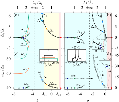
Figure 1: (Color online) Dynamical phase diagrams for the constant DOS (left) and the graphene-like DOS model (right) as schematized in the white background insets. The lower scale shows the control parameter $\delta$ while the upper scale is non-linear and shows $\lambda_{f}/\lambda_{i}$ for the particular case, $W=40\Delta_{i}$. Panels (a) and (b) show extreme values of the order parameter characterizing the dynamics, while the lower panel shows the frequency of the Higgs oscillations labeled by the corresponding singularities in the quasiparticle DOS (see text). The background color indicates the different dynamical regimes: synchronized (magenta), damped oscillations (yellow) and overdamped (red). Full lines are obtained from the Lax root analysis, while circles are from numerical simulations (full circles correspond to dynamics shown in detail in other figures). The dashed line fitting the $\omega_{l}$ frequency is $2\bar{\Delta}$ from the simulations, while the line is $2\Delta_{\infty}$ from the Lax root analysis. The dashed line fitting $\omega_{V}$ indicates $2\xi_{\bm{k}}^{V}$. Both $\omega_{l}$ and $\omega_{V}$ correspond to the right scale, as indicated by the arrows. The colored background insets are zoomed to the indicated regions.

Dynamical Phase diagram. In Fig. 1 we present the dynamical phase diagram for three different bandwidths and a constant DOS (left) and for the graphene-like DOS (right). Panels (a) and (b) show key values of the order parameter characterizing the dynamics, while panels (c) and (d) show the generalized SHP oscillation frequencies. Full lines were obtained exploiting the integrability of the model through a Lax roots analysis (see Supplementary Information, SI for details) and were checked by numerical simulations (circles). The frequencies of Higgs modes are labeled according to a singularity of the quasiparticle DOS to which we show below to be associated, namely, lower edge (l), upper edge (u), Van Hove (V) and Dirac point (D).

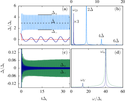
Figure 2: (Color online) Representative dynamics (left column) and their FT (right column) for the graphene-like DOS case. (a) Different time dependence of superconducting order parameter for quenches in the attractive side $\lambda_{f}/\lambda_{i}>0$ (non-critical quenches). The magenta and dark-blue curves correspond to synchronized phases, while we show in red a typical dynamics in the overdamped regime. The FT are shown in the panel (b) where peaks related to Higgs mode $2\bar{\Delta}$ (and high harmonics) as well as $\omega_{D}$ appear. (c) Two $\Delta(t)$ for CQ $(\lambda_{f}/\lambda_{i}<0)$ and their respective FT in (d). Here, in addition to the strong response with frequency $\omega_{u}\simeq W$ also a frequency $\omega_{V}$ emerges. This Higgs mode is related to the Van-Hove singularities in the graphene-like DOS (see text). The quench parameters, $\delta$ used for each curve, correspond to the colored full circles of Fig. 1. In all cases the FT show finite width peaks due to the finite time windows we have considered: $t\Delta_{i}\in\left[5,50\right]$ in all the cases except to resolve the slow Dirac-Higgs mode [dark blue curves in panels (a) and (b)] for which we use $t\Delta_{i}\in\left[5,300\right]$.

In Fig. 1 the curves to the right of the vertical dashed line in panel (a) and (c) reproduce the results of Ref. Barankov2006a where three dynamical phases were found for non-critical quenches $\lambda_{f}/\lambda_{i}>0$ (see SI Fig. S1 for details of the dynamics at colored dots): For small increase and decrease of the attraction in the quench (small $|\delta|$), the superconducting order parameter shows damped oscillations with a Higgs frequency associated with the lower edge of the quasiparticle DOS, $\omega_{l}=2\Delta_{\infty}$ and saturates to a constant value $\Delta_{\infty}$ at long times which therefore coincides with $\bar{\Delta}$ (yellow shading). For large quenches there are two possible outcomes. Decreasing the pairing constant beyond a critical point ($\delta>\delta_{c+}=\pi/2$), the system goes to a gapless regime ($\Delta_{\infty}=0$) with an overdamped dynamics (red region). Increasing the pairing above a critical point ($\delta<\delta_{c-}=-\pi/2$), the system synchronizes and the order parameter oscillates between the values $\Delta_{+}$ and $\Delta_{-}$ with a fundamental Higgs frequency equal to twice the average order parameterSeibold2020 , $\omega_{l}=2\bar{\Delta}$ (magenta area). We will refer to this well known phenomenaBarankov2004 ; Barankov2006a ; Collado2019 as the “lower-edge SHP”.

Using $\delta$ as the control parameter has the advantage that for large enough bandwidth, the results for $\lambda_{f}/\lambda_{i}>0$ become independent of the bandwidth, so the curves for different $W$ fall almost on top of each other. Thus, the dynamical phases obtained after non-critical quenches display a certain degree of universality, which is correctly captured in terms of the variable $\delta$. The upper scale (and the position of the vertical dashed line) corresponds to the particular case, $W/\Delta_{i}=40$. The region close to the vertical dashed line has a final interaction in the strong coupling regime which is out of our scope, so data is omitted.

The region to the left of the vertical dashed line shows the result of the CQ. A different synchronized regime is found where the order parameter oscillates with symmetric amplitudes $\Delta_{+}$ and $\Delta_{-}$ around zero instead of having a finite average $\bar{\Delta}$ [see SI Fig. S1(c) for the detailed dynamics at the colored dots]. This zero order-parameter average (ZOPA) behavior is reminiscent of the time-crystal phases found with periodic driving Collado2021 . In contrast to the purely attractive interaction quench, the amplitudes and the Higgs frequency are strongly dependent on the bandwidth. In this case, the SHP frequency converges to the upper edge of the fluctuation DOS ($\omega_{u}\rightarrow W$), when the final interaction is repulsive and small (large negative $\delta$). For $\delta<-8$ (large repulsive $\lambda_{f}$) the amplitude becomes vanishing small and the dynamical phase can not be distinguished from a gapless state. Therefore, for large negative and positive $\delta$ ($\lambda_{f}\rightarrow\pm 0$) the system converges to the same gapless phase.

The occurrence of SHP associated with upper and lower edges of the fluctuation/quasiparticle DOS suggests that singularities act as nucleation centers in frequency space to stabilize the synchronized phases during the non-linear dynamics. We expect this mechanism to be ubiquitous, thus leading to the appearance of Higgs mode signatures in any conventional superconducting system with singular DOS. In order to confirm this expectation, we have studied the dynamical phase diagram of a Dirac system with a graphene-like DOS (right column) where two additional singularities are present already in the bare DOS: one at the Fermi level (Dirac point) and the Van Hove singularities at $\xi_{\bm{k}}^{V}\approx\pm 6.66\Delta_{i}$ (see DOS in the white background inset of Fig. 1).

Interestingly, the phase diagram of the graphene-like model turns out to be quite different from the flat-DOS case. The damped regime (yellow region) is completely absent and synchronization occurs even for an arbitrary small quench [see zoomed region inset in Fig. 1(b) and the detailed dynamics at the light blue point in Fig. 2(a)]. Also, differently from the constant DOS model, the synchronization phenomenon takes place both for an increase and a decrease of the pairing interaction. In the latter case, decreasing enough $\lambda_{f}$, the pseudospins effectively decouple from each other and the gapless regime is recovered (red region). A representative dynamics of this phase is shown in Fig. 2(a) in red using the parameters indicated with red circle in Fig. 1 (b).

Between the $\delta=0$ and the gapless phase, a quite rich transition is found, as shown in the zoomed insets of panel (b) and (d) of Fig. 1. First, twice the average order parameter (thin dashed line) and the frequency $\omega_{l}$ decrease very rapidly tracking each other, as in other non-ZOPA synchronized phases, until a critical value $\delta_{c1}=0.07$ where both are driven to zero. Beyond this $\delta_{c1}$, a ZOPA synchronized phase appears associated to the Dirac point singularity with a frequency $\omega_{D}$ as shown in dark blue in Fig. 2 (a) and (b). This dynamical phase is stable in a very narrow window with the frequency $\omega_{D}$ increasing with $\delta$ until it collapses in the overdamped phase at a second critical value $\delta_{c2}=0.22$.

The Fourier transform (FT) of the dynamics shown in panel (b) of Fig. 2 reveal that in the lower-edge SHP, the graphene-like model shows up to three harmonics while in the flat DOS model only two harmonics are visible for the present parameters [SI Fig. S1(b)]. The synchronized Dirac-Higgs phase, in contrast, appears much more harmonic.

Panel (c) and (d) of Fig. 2 exemplify the dynamics for the CQ corresponding to the matching full dots in Fig. 1 (b), (d), where the upper-edge SHP is excited. The overall appearance is very similar to the case of a flat DOS [SI Fig. S1 (b), (d)] showing ZOPA behavior. However, an extra weak modulation appears, which is revealed as a new frequency $\omega_{V}$ in the Fourier transform (d). This frequency matches twice the Van Hove singularity in the DOS $2\xi_{\bm{k}}^{V}$, thus as expected, a synchronized Van Hove-Higgs mode can be excited. Its amplitude decreases in time, indicating that the mode is damped, although with quite a long coherence time, as witnessed by the narrow peak in the FT.

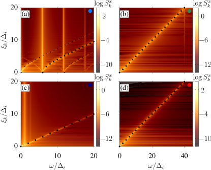
Figure 3: (Color online) FT of the x-component of pseudospin texture for each of the dynamical phases assuming a graphene-like DOS. The parameter $\delta$ for each panel corresponds to the full colored circle in Figs. 1 and 2. For all panels $\lambda_{f}/\lambda_{i}>0$ except for the right upper panel (b) in which the synchronization phenomenon (unveiled as a vertical intensity line close to $\omega=40\Delta_{i}$) occurs by quenching to repulsive interaction $\lambda_{f}/\lambda_{i}<0$ (CQ). The FT were computed using a time window $t\Delta_{i}\in\left[0,100\right]$.

To fully characterizes the dynamical phases and the emergence of synchronization in the system, it is instructive to analyze the $\xi_{\bm{k}}$-resolved FT of the pseudospin dynamics. As we are interested in the pairing dynamics, we show the FT of the $x$-component of pseudospins for the graphene-like model in Fig. 3 (SI Fig. S2 shows the same information for the flat DOS model).

Single-particle (pseudospin) excitations appear as dispersive features, while synchronized collective modes appear as vertical lines. For the non-ZOPA synchronized phase (light blue dots in Fig. 1) single-particle excitations appear in the dynamics as Larmor precessions with frequency $\Omega_{L}(\bm{k})=2\sqrt{\xi_{\bm{k}}^{2}+\bar{\Delta}^{2}}$ as shown in panel Fig. 3(a) with the large black dots. The same panel shows that the lower edge Higgs mode is not determined only by the quasiparticles participating in the edge singularity of $\Omega_{L}(\bm{k})$ at the frequency $2\bar{\Delta}$. Indeed, the vertical feature emerging from $2\bar{\Delta}$ witnesses that all quasiparticles in this $\xi_{\bm{k}}$ window are synchronized and participate in the collective mode. Thus, the edge singularity of the dispersion can be seen as a nucleation center in frequency space given a “rhythm” which is followed by the rest of the quasiparticles due to the interactions.

In addition, of the main $\Omega_{L}(\bm{k})$ dispersion, Floquet side bands appear analogous to the bands observed under periodic drive Collado2021 . Here, of course, an external periodic drive is not present and the bands are self-generated by the action of the lower-edge Higgs mode with frequency $\omega_{l}$ yielding replicas at $\Omega_{L}(\bm{k})+n\omega_{l}$ with $n=-1,0,1,2,...$ and weaker features at $-\Omega_{L}(\bm{k})+n\omega_{l}$ with $n=0,1$.

Panel (b) shows that the upper edge singularity of the DOS is enough to trigger the SHP (appearing as a vertical feature) with frequency $\omega_{u}\simeq W$ provided that the appropriate protocol, i.e. the CQ, is used. Thus, the $1/\sqrt{\omega-2\bar{\Delta}}$ divergence present at the lower edge of the DOS is not a prerequisite to stabilize Higgs modes. No feature associated with the Van Hove-Higgs mode $\omega_{V}$ can be seen here, since the numerical analysis has been performed on a time window larger than its coherence time in order to have high-frequency resolution.

In panel (b) the ZOPA manifests as a gapless linear dispersion of single particle excitations, $\Omega_{L}(\bm{k})=2\xi_{\bm{k}}$ (black dots). The same linear dispersion appears for the other ZOPA modes: the Dirac-Higgs shown in panel (c) and the gapless mode shown in (d). For the former, the collective nature of the synchronization is also evident from the vertical feature at $\omega_{D}$.

Conclusions. We have shown that different synchronized Higgs phases can be excited in a BCS system by choosing an appropriate quench protocol. For a given system, the frequency of the mode is determined by singularities in the DOS with small corrections due to quasiparticle interactions. The previously known lower-edge Higgs mode appears at the same frequency of a singularity in the equilibrium particle-particle response. The upper edge SHP is reminiscent of antibound states appearing in the equilibrium pairing response of repulsive systems. However, at equilibrium the mode is not present in particle-hole symmetric situations Seibold2008 while here the mode is stabilized in an out-of-equilibrium setting. Thus, generalized Higgs modes do not appear to have always an equilibrium counterpart.

Our findings provide an innovative interpretation to the Higgs mode dynamics, which appear as synchronized quasiparticles oscillations nucleated by DOS singularities. This, in turns, implies that any spectral singularity can give rise to Higgs-mode like oscillations given a suitable quench.

The observation of the previously reported lower-edge SHP in real superconductors is hindered by its decay in other excitations and its weak coupling to light podolsky2011visibility ; scott2012rapid ; Cea2015 ; Collado2019 . Furthermore, signatures of Higgs dynamics in pump and probe experiments Matsunaga2013 ; Matsunaga2014 ; buzzi2021higgs cannot be clearly distinguished from other Raman active modesMansart2013 with similar frequencies, but different underlying mechanisms. The experimental detection of other Higgs modes presented here will probably encounter similar difficulties in solid state systems, as our picture is based on the BCS model, whose integrable nature does not account for thermalization.

A proper understanding of the generalized Higgs dynamics and its decay at strong coupling, as well as the possible relation with the equilibrium characteristic of the SSB phase, may be obtained by direct observation in Fermi superfluids of cold atoms. Indeed, recent improvements in the control and observation of ultracold atoms in optical lattices goldman2016topological ; gross2017quantum allowed the study of both equilibrium and transport properties of Fermi systems on the lattice mazurenko2017cold ; koespell2019imaging ; brown2019bad ; nichols2019spin , paving the way to the realization of the generalized Higgs dynamics described here. In particular, an artificial graphene-like lattice with tunable interactions has been realized Uehlinger2013 . Another route is to use cold atoms in an optical cavity, which has recently been proposed as a BCS simulator Lewis-Swan2021 .

Interestingly, the search for more than one Higgs boson is a subject of intense search also in high-energy scattering experiments Tumasyan2021 . This kind of probes, however, are more akin to equilibrium responses in condensed matter. Instead, the strongly out-of-equilibrium physics investigated here may find parallels in the electroweak transition of relevance for early universe cosmology and baryogenesis Ghosh2016 .

- (1) Y. Nambu and G. Jona-Lasinio, Phys. Rev. 122, 345 (1961).
- (2) S. Sachdev, Quantum Phase Transitions (Cambridge University Press, Cambridge, 2011), pp. 1–517.
- (3) C. Di Castro and R. Raimondi, Statistical Mechanics and Applications in Condensed Matter (Cambridge University Press, Cambridge, UK, 2015).
- (4) H. Nishimori and G. Ortiz, Elements of Phase Transitions and Critical Phenomena, Oxford Graduate Texts (Oxford University press, Oxford, UK, 2011).
- (5) P. W. Anderson, Phys. Rev. 130, 439 (1963).
- (6) F. Englert and R. Brout, Phys. Rev. Lett. 13, 321 (1964).
- (7) P. W. Higgs, Phys. Rev. Lett. 13, 508 (1964).
- (8) G. S. Guralnik, C. R. Hagen, and T. W. B. Kibble, Phys. Rev. Lett. 13, 585 (1964).
- (9) T. W. B. Kibble, Scholarpedia 4, 6441 (2009), revision #91222.
- (10) L. Álvarez-Gaumé and J. Ellis, Nature Physics 7, 2 (2011).
- (11) L. N. Cooper, Phys. Rev. 104, 1189 (1956).
- (12) J. Bardeen, L. N. Cooper, and J. R. Schrieffer, Phys. Rev. 108, 1175 (1957).
- (13) R. Sooryakumar and M. V. Klein, Phys. Rev. Lett. 45, 660 (1980).
- (14) C. A. Balseiro and L. M. Falicov, Phys. Rev. Lett. 45, 662 (1980).
- (15) P. B. Littlewood and C. M. Varma, Phys. Rev. Lett. 47, 811 (1981).
- (16) T. Cea and L. Benfatto, Phys. Rev. B - Condens. Matter Mater. Phys. 90, 224515 (2014).
- (17) R. Grasset, T. Cea, Y. Gallais, M. Cazayous, A. Sacuto, L. Cario, L. Benfatto, and M.-A. Méasson, Phys. Rev. B 97, 094502 (2018).
- (18) C. Rüegg, B. Normand, M. Matsumoto, A. Furrer, D. F. McMorrow, K. W. Krämer, H. U. Güdel, S. N. Gvasaliya, H. Mutka, and M. Boehm, Phys. Rev. Lett. 100, 205701 (2008).
- (19) W. P. Halperin and E. Varoquaux, in Helium Three, Vol. 26 of Modern Problems in Condensed Matter Sciences, edited by W. P. Halperin and L. P. Pitaevskii (Elsevier, Amsterdam, Netherlands, 1990), pp. 353–522.
- (20) R. Matsunaga, Y. I. Hamada, K. Makise, Y. Uzawa, H. Terai, Z. Wang, and R. Shimano, Phys. Rev. Lett. 111, 057002 (2013).
- (21) R. Matsunaga, N. Tsuji, H. Fujita, A. Sugioka, K. Makise, Y. Uzawa, H. Terai, Z. Wang, H. Aoki, and R. Shimano, Science 345, 1145 (2014).
- (22) D. Sherman, U. S. Pracht, B. Gorshunov, S. Poran, J. Jesudasan, M. Chand, P. Raychaudhuri, M. Swanson, N. Trivedi, A. Auerbach, M. Scheffler, A. Frydman, and M. Dressel, Nature Physics 11, 188 (2015).
- (23) K. Katsumi, N. Tsuji, Y. I. Hamada, R. Matsunaga, J. Schneeloch, R. D. Zhong, G. D. Gu, H. Aoki, Y. Gallais, and R. Shimano, Phys. Rev. Lett. 120, 117001 (2018).
- (24) H. Chu, M.-J. Kim, K. Katsumi, S. Kovalev, R. D. Dawson, L. Schwarz, N. Yoshikawa, G. Kim, D. Putzky, Z. Z. Li, H. Raffy, S. Germanskiy, J.-C. Deinert, N. Awari, I. Ilyakov, B. Green, M. Chen, M. Bawatna, G. Cristiani, G. Logvenov, Y. Gallais, A. V. Boris, B. Keimer, A. P. Schnyder, D. Manske, M. Gensch, Z. Wang, R. Shimano, and S. Kaiser, Nat. Commun. 11, 1793 (2020).
- (25) R. Shimano and N. Tsuji, Annu. Rev. Condens. Matter Phys. 11, 103 (2020).
- (26) T. Cea, C. Castellani, G. Seibold, and L. Benfatto, Phys. Rev. Lett. 115, 157002 (2015).
- (27) T. Cea, C. Castellani, and L. Benfatto, Phys. Rev. B 93, 180507 (2016).
- (28) S. Gazit, D. Podolsky, and A. Auerbach, Phys. Rev. Lett. 110, 140401 (2013).
- (29) M. Silaev, Phys. Rev. B 99, 224511 (2019).
- (30) Y. Murotani and R. Shimano, Phys. Rev. B 99, 224510 (2019).
- (31) U. Bissbort, S. Götze, Y. Li, J. Heinze, J. S. Krauser, M. Weinberg, C. Becker, K. Sengstock, and W. Hofstetter, Phys. Rev. Lett. 106, 205303 (2011).
- (32) M. Endres, T. Fukuhara, D. Pekker, M. Cheneau, P. Schauß, C. Gross, E. Demler, S. Kuhr, and I. Bloch, Nature (London) 487, 454 (2012).
- (33) T. M. Hoang, H. M. Bharath, M. J. Boguslawski, M. Anquez, B. A. Robbins, and M. S. Chapman, Proceedings of the National Academy of Sciences 113, 9475 (2016).
- (34) J. Léonard, A. Morales, P. Zupancic, T. Donner, and T. Esslinger, Science 358, 1415 (2017).
- (35) D. Podolsky, A. Auerbach, and D. P. Arovas, Phys. Rev. B 84, 174522 (2011).
- (36) R. G. Scott, F. Dalfovo, L. P. Pitaevskii, and S. Stringari, Phys. Rev. A 86, 053604 (2012).
- (37) Y. Barlas and C. Varma, Phys. Rev. B 87, 054503 (2013).
- (38) B. Liu, H. Zhai, and S. Zhang, Phys. Rev. A 93, 033641 (2016).
- (39) X. Han, B. Liu, and J. Hu, Phys. Rev. A 94, 033608 (2016).
- (40) A. Behrle, T. Harrison, J. Kombe, K. Gao, M. Link, J. S. Bernier, C. Kollath, and M. Köhl, Nature Physics 14, 781 (2018).
- (41) J. Bjerlin, S. M. Reimann, and G. M. Bruun, Phys. Rev. Lett. 116, 155302 (2016).
- (42) L. Bayha, M. Holten, R. Klemt, K. Subramanian, J. Bjerlin, S. M. Reimann, G. M. Bruun, P. M. Preiss, and S. Jochim, Nature (London)587, 583 (2020).
- (43) M. Heyl, Reports Prog. Phys. 81, 054001 (2018).
- (44) M. Eckstein, M. Kollar, and P. Werner, Phys. Rev. Lett. 103, 056403 (2009).
- (45) J. P. Garrahan and I. Lesanovsky, Phys. Rev. Lett. 104, 160601 (2010).
- (46) S. Diehl, A. Tomadin, A. Micheli, R. Fazio, and P. Zoller, Phys. Rev. Lett. 105, 015702 (2010).
- (47) M. Schiró and M. Fabrizio, Phys. Rev. Lett. 105, 076401 (2010).
- (48) B. Sciolla and G. Biroli, Phys. Rev. Lett. 105, 220401 (2010).
- (49) M. Heyl, A. Polkovnikov, and S. Kehrein, Phys. Rev. Lett. 110, 135704 (2013).
- (50) M. Heyl, Phys. Rev. Lett. 115, 140602 (2015).
- (51) P. Jurcevic, H. Shen, P. Hauke, C. Maier, T. Brydges, C. Hempel, B. P. Lanyon, M. Heyl, R. Blatt, and C. F. Roos, Phys. Rev. Lett. 119, 080501 (2017).
- (52) J. Zhang, G. Pagano, P. W. Hess, A. Kyprianidis, P. Becker, H. Kaplan, A. V. Gorshkov, Z. X. Gong, and C. Monroe, Nature (London)551, 601 (2017).
- (53) B. Zunkovic, M. Heyl, M. Knap, and A. Silva, Phys. Rev. Lett. 120, 130601 (2018).
- (54) J. C. Halimeh and V. Zauner-Stauber, Phys. Rev. B 96, 134427 (2017).
- (55) J. C. Halimeh, V. Zauner-Stauber, I. P. McCulloch, I. de Vega, U. Schollwöck, and M. Kastner, Phys. Rev. B 95, 024302 (2017).
- (56) N. Defenu, T. Enss, and J. C. Halimeh, Phys. Rev. B 100, 014434 (2019).
- (57) P. Uhrich, N. Defenu, R. Jafari, and J. C. Halimeh, Phys. Rev. B 101, 245148 (2020).
- (58) R. A. Barankov, L. S. Levitov, and B. Z. Spivak, Phys. Rev. Lett. 93, 160401 (2004).
- (59) R. A. Barankov and L. S. Levitov, Phys. Rev. Lett. 96, 230403 (2006).
- (60) P. W. Anderson, Phys. Rev. 112, 1900 (1958).
- (61) H. P. Ojeda Collado, G. Usaj, J. Lorenzana, and C. A. Balseiro, Phys. Rev. B 99, 174509 (2019).
- (62) H. P. O. Collado, J. Lorenzana, G. Usaj, and C. A. Balseiro, Phys. Rev. B 98, 214519 (2018).
- (63) H. P. Ojeda Collado, G. Usaj, C. A. Balseiro, D. H. Zanette, and J. Lorenzana, Phys. Rev. Res. 3, L042023 (2021).
- (64) M. Mootz, J. Wang, and I. E. Perakis, Phys. Rev. B 102, 45 (2020).
- (65) Y.-Z. Chou, Y. Liao, and M. S. Foster, Phys. Rev. B 95, 104507 (2017).
- (66) G. Seibold and J. Lorenzana, Phys. Rev. B 102, 144502 (2020).
- (67) G. Seibold, F. Becca, and J. Lorenzana, Phys. Rev. Lett. 100, 016405 (2008).
- (68) M. Buzzi, G. Jotzu, A. Cavalleri, J. I. Cirac, E. A. Demler, B. I. Halperin, M. D. Lukin, T. Shi, Y. Wang, and D. Podolsky, Phys. Rev. X 11, 011055 (2021).
- (69) B. Mansart, J. Lorenzana, a. Mann, a. Odeh, M. Scarongella, M. Chergui, and F. Carbone, Proc. Natl. Acad. Sci. 110, 4539 (2013).
- (70) N. Goldman, J. C. Budich, and P. Zoller, Nat. Phys. 12, 639 (2016).
- (71) C. Gross and I. Bloch, Science 357, 995 (2017).
- (72) A. Mazurenko, C. S. Chiu, G. Ji, M. F. Parsons, M. Kanász-Nagy, R. Schmidt, F. Grusdt, E. Demler, D. Greif, and M. Greiner, Nature 545, 462 (2017).
- (73) J. Koepsell, J. Vijayan, P. Sompet, F. Grusdt, T. A. Hilker, E. Demler, G. Salomon, I. Bloch, and C. Gross, Nature 572, 358 (2019).
- (74) P. T. Brown, D. Mitra, E. Guardado-Sanchez, R. Nourafkan, A. Reymbaut, C.-D. Hébert, S. Bergeron, A. M. S. Tremblay, J. Kokalj, D. A. Huse, P. Schauß, and W. S. Bakr, Science 363, 379 (2019).
- (75) M. A. Nichols, L. W. Cheuk, M. Okan, T. R. Hartke, E. Mendez, T. Senthil, E. Khatami, H. Zhang, and M. W. Zwierlein, Science 363, 383 (2019).
- (76) T. Uehlinger, G. Jotzu, M. Messer, D. Greif, W. Hofstetter, U. Bissbort, and T. Esslinger, Phys. Rev. Lett. 111, 185307 (2013).
- (77) R. J. Lewis-Swan, D. Barberena, J. R. K. Cline, D. J. Young, J. K. Thompson, and A. M. Rey, Phys. Rev. Lett. 126, 173601 (2021).
- (78) A. Tumasyan et al., J. High Energy Phys. 2021, 57 (2021).
- (79) B. Ghosh, Pramana 87, 43 (2016).