Constraining Feeble Neutrino Interactions with Ultralight Dark Matter

Abstract

If ultralight $(\ll$ eV), bosonic dark matter couples to right handed neutrinos, active neutrino masses and mixing angles depend on the ambient dark matter density. When the neutrino Majorana mass, induced by the dark matter background, is small compared to the Dirac mass, neutrinos are “pseudo-Dirac” fermions that undergo oscillations between nearly degenerate active and sterile states.

We present a complete cosmological history for such a scenario and find severe limits from a variety of terrestrial and cosmological observables. For scalar masses in the “fuzzy” dark matter regime ($\sim 10^{-20}$ eV), these limits exclude couplings of order $10^{-30}$, corresponding to Yukawa interactions comparable to the gravitational force between neutrinos and surpassing equivalent limits on time variation in scalar-induced electron and proton couplings.

I Introduction

Ultralight $(\ll$ eV) bosonic dark matter (DM) $\phi$ is characterized by a macroscopic de-Broglie wavelength

$$\lambda_{\phi}=\frac{1}{m_{\phi}v_{\phi}}\approx 200{\rm\,km}\left(\frac{\rm neV}{m_{\phi}}\right)\left(\frac{10^{-3}}{v_{\phi}}\right),$$ (1)

which exceeds the inter-particle separation, where $v_{\phi}$ is the field veloctiy. If $\phi$ is misaligned from the minimum of quadratic potential, it oscillates as a classical field about this minimum according to

$$\phi(\vec{r},t)=\frac{\sqrt{2\rho_{\phi}(t)}}{m_{\phi}}\cos[m_{\phi}(t+\vec{v}_{\phi}\cdot\vec{r}\,)+\varphi(\vec{r}\,)]~{},$$ (2)

and the corresponding energy density redshifts like non-relativistic matter $\rho_{\phi}\propto a^{-3}$, where $a$ is the cosmic scale factor and $\varphi$ is a possible phase. This phase may encode additional information about spatial variation – e.g. different $\phi$ domains arising from cosmological initial conditions or the incoherent virialization in the Galaxy leading to variation on the scale of $\lambda_{\phi}$.

If $\phi$ couples to Standard Model (SM) particles, their masses, spins, and coupling constants may inherit time dependence from Eq. (2). In the context of charged SM particles, there are many searches for such phenomena, which typically place very strong limits on the $\phi$-SM interaction strength (see Ref. [1] for a review). By contrast, there are relatively few bounds on DM induced time dependence in the neutrino sector [2, 3, 4, 5, 6, 7, 8, 9, 10, 11, 12, 13, 14, 15] and the corresponding limits constrain comparatively large interaction strengths primarily via flavor oscillations.

In this paper we introduce the possibility that an ultralight DM candidate $\phi$ induces a time dependent Majorana mass for right-handed neutrinos

$$m_{M}=\frac{y_{\phi}}{2}\phi(t),$$ (3)

where $y_{\phi}$ is a coupling constant and the time dependence arises from Eq. (2). When this mass is small compared to the neutrino Dirac mass $m_{D}$, the mass eigenstates form a pair of pseudo-Dirac fermions; one “active” $\nu_{a}$ and one “sterile” $\nu_{s}$ (per generation). These states oscillate into each other with a characteristic probability governed by their squared mass difference $\delta m^{2}$ [16]

$$P(\nu_{a}\to\nu_{s})=\sin^{2}(2\theta)\sin^{2}\left(\frac{\delta m^{2}L}{4E_{\nu}}\right),$$ (4)

where $L$ is the baseline, $E_{\nu}$ is the energy of the propagating neutrino, and $\theta\approx\pi/4$ is the mixing angle, which is near maximal in the pseudo-Dirac limit where $m_{M}\ll m_{D}$.

The Majorana mass governing $\delta m^{2}$ in Eq. (4) is time dependent, so the oscillation rate becomes sensitive to the dark matter density and to its cosmic evolution. This dependence can impact various terrestrial and cosmological observables. In this work we extract resultant bounds and impose extremely strong limits on the induced Majorana mass; depending on the value of $m_{\phi}$ we find some limits on the coupling $y_{\phi}$ corresponding to a $\phi$ mediated Yukawa force comparable to that of gravity.

This letter is organized as follows: in section II we present our theoretical framework, in section III we delineate the qualitatively different neutrino oscillation regimes that $\phi$ can induce, in section IV we compute the terrestrial bounds, in section V we determine the cosmological bounds on this scenario, and in VI we make some concluding remarks.

II Ultralight dark matter and pseudo-Dirac neutrinos

We consider a scalar DM candidate $\phi$ with lepton number 2 and a cosmic abundance due to misalignment. In Weyl fermion notation, the Lagrangian in this scenario contains

$$\mathcal{L}\supset y_{\nu}H\ell N+\frac{y_{\phi}}{2}\phi NN+h.c.~{},$$ (5)

where $y_{\nu}$ is the neutrino Yukawa coupling, $H$ is the SM Higgs doublet, $\ell$ is the SM lepton doublet, and $N$ is a SM neutral fermion, i.e. a right-handed neutrino. As we will see next, the presence of a feeble interaction between the scalar DM and the right-handed neutrino can have dramatic effects in neutrino oscillation phenomenology.

To understand the impact of $\phi$ on neutrino oscillations, it is instructive to describe the “1+1” scenario, in which there is only one generation of $\ell$ and $N$. For simplicity, assume that the active state here is an electron flavor neutrino. In the broken electroweak phase, the first term in Eq. (5) generates a Dirac mass of neutrinos. When the $\phi$ field is misaligned according to Eq. (2), the second term in Eq. (5) generates a Majorana mass for $N$, so we have

$$m_{D}=\frac{y_{\nu}v}{\sqrt{2}}~{}~{},~{}~{}m_{M}=\frac{y_{\phi}}{2}\phi(t)~{},$$ (6)

for the Dirac and Majorana contributions, respectively, where $v=246$ GeV is the Higgs vacuum expectation value.

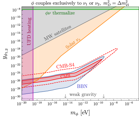
Figure 1: Left: Parameter space for $\phi$ coupled only to $\nu_{1}$ or $\nu_{2}$ mass eigenstates, which is predominantly constrained $\nu_{e}$ oscillation bounds. Here we show bounds from CMB and BBN from Sec. V, Milky Way satellites from Sec. V.2, scalar thermalization with neutrinos from Sec. V.3, solar neutrino oscillations from Sec. IV.1, and model independent limits on light DM from ultra faint dwarf (UFD) heating [17]. For points below the gray dotted line, the $\phi$ mediated force between right handed neutrinos is weaker than gravity, which is theoretically disfavored by the weak gravity conjecture [18] Right: same as the left panel, only $\phi$ now couples only to $\nu_{3}$, so the limits are driven by $\nu_{\mu,\tau}$ oscillations for which the solar bound is subdominant to the atmospheric bound described in Sec. IV.2.

When $m_{M}\ll m_{D}$, we obtain two nearly degenerate neutrino mass-squared eigenstates

$$m^{2}_{h,\ell} =m_{D}^{2}\pm m_{D}m_{M}\equiv m^{2}_{\nu}\pm\frac{1}{2}\delta m^{2}~{},$$ (7)

and we define $\delta m^{2}\equiv y_{\phi}m_{D}\sqrt{2\rho_{\phi}}/m_{\phi}$, where

$$\delta m^{2}\approx 2\!\times\!10^{-15}{\rm eV^{2}}\!\left(\frac{y_{\phi}}{10^{-10}}\right)\!\left(\frac{10^{-15}{\rm eV}}{m_{\phi}}\right)\left(\frac{m_{D}}{0.1\,\rm eV}\right),~{}~{}~{}$$ (8)

for the splitting between Weyl fermions as opposed to the usual $\Delta m^{2}_{ij}$ measured in oscillation experiments; here we have taken the local density to be $\rho^{\odot}_{\phi}=0.4$ GeV/cm³ [19]. The active-sterile mixing angle in this case is

$$\tan\left(2\theta\right)=\frac{2m_{D}}{m_{M}}\gg 1~{},$$ (9)

which is nearly maximal, $\theta\approx\pi/4$ in our full parameter space of interest.

The diagonalization of the mass terms in Eq. (6) is obtained by defining the flavor fields in terms of the mass eigenstates approximately as

$$|\nu_{e}\rangle= \frac{1}{\sqrt{2}}\bigl{(}|\nu_{h}\rangle+|\nu_{\ell}\rangle\bigr{)},$$ (10)

$$|\nu_{s}\rangle= \frac{1}{\sqrt{2}}\bigl{(}|\nu_{h}\rangle-|\nu_{\ell}\rangle\bigr{)}.$$ (11)

The time evolution of a $\nu_{e}$ state is given by

$$U(t)|\nu_{e}\rangle = \frac{1}{\sqrt{2}}\biggl{[}\exp\left(-\frac{i}{2E_{\nu}}\int_{0}^{t}\!dt^{\prime}m_{1}^{2}(t^{\prime})\right)|\nu_{1}\rangle$$ (12)

$$~{}~{}~{}+\exp\left(-\frac{i}{2E_{\nu}}\int_{0}^{t}\!dt^{\prime}m_{2}^{2}(t^{\prime})\right)|\nu_{2}\rangle\biggr{]},~{}~{}$$

which yields a $\nu_{e}\to\nu_{e}$ survival probability

$$P_{ee}(t)=|\langle\nu(t)|\nu_{e}\rangle|^{2}=\cos^{2}\left(\frac{1}{4E_{\nu}}\int_{0}^{t}dt^{\prime}\delta m^{2}(t^{\prime})\right).~{}~{}~{}~{}~{}$$ (13)

Using Eqs. (2) and (6) we obtain

$$\frac{1}{2}\int_{0}^{t}dt^{\prime}\delta m^{2}(t^{\prime})=\frac{y_{\phi}m_{D}}{m_{\phi}}\sqrt{2\rho_{\phi}}\int_{0}^{t}dt^{\prime}\cos\left(m_{\phi}t^{\prime}+\varphi\right),$$ (14)

where we have absorbed the $v_{\phi}$ dependence in Eq. (2) into the definition of $\varphi$ for brevity. Thus, for a neutrino emitted at $t=0$ and observed at some later time $t$, the resulting electron-neutrino disappearance probability can be written as

$$1\!-\!P_{ee}=\sin^{2}\!\left\{\frac{m_{D}}{2E_{\nu}}\frac{y_{\phi}\sqrt{2\rho_{\phi}}}{m^{2}_{\phi}}\biggl{(}\sin\left[m_{\phi}t+\varphi\right]\!-\sin\varphi\biggr{)}\!\right\},~{}~{}~{}~{}~{}~{}$$ (15)

where we have treated the phase $\varphi$ as a constant over the propagation time.

Generalization for more neutrino flavors is straightforward and can be derived following similar steps as those taken in Ref. [20]. Moreover, to simplify the discussion on the constraints and because the electron-neutrino admixture in $\nu_{3}$ is small ($|U_{e3}|\ll 1$), when $\phi$ couples to $\nu_{1}$ or $\nu_{2}$ we will only consider nonstandard $\nu_{e}$ disappearance, while when $\phi$ couples to $\nu_{3}$ we will only consider nonstandard $\nu_{\mu,\tau}$ disappearance; in both regimes, we treat the active-sterile oscillation in a two-flavor (active-sterile) framework.

As written in Eq. (2), the phase $\varphi$ need not be constant over the full neutrino trajectory. Indeed, in the Galaxy, virialization will disrupt any constant phase value down to coherence patches of order the de-Broglie wavelength in Eq. (1). Thus, the full oscillation probability will depend crucially on the relative size of the oscillation baseline and this coherence scale.

Finally, we note that our scalar mass is not protected by any symmetry, so it will be sensitive to irreducible one-loop corrections of order

$$\delta m_{\phi}\sim\frac{y_{\phi}m_{D}}{4\pi}\sim 10^{-18}\,{\rm eV}\left(\frac{y_{\phi}}{10^{-15}}\right)\left(\frac{m_{D}}{10\,\rm meV}\right),~{}$$ (16)

from the interactions in Eq. (5). Thus, for small $y_{\phi}$ in the pseudo-Dirac limit, this contribution does not destabilize the ultralight scalar mass, assuming no $\phi$ couplings to heavier states.

III Neutrino Oscillation Regimes

In what follows, we will consider three distinct regimes for neutrino oscillations in the presence of the ultralight scalar fields. These regimes arrive from the relation between the neutrino oscillation length and the modulation frequency of $\phi$ or the coherence length that defines the overall phase $\varphi$. Instead of performing a detailed fit of experimental data, we will recast existing constraints on pseudo-Dirac neutrinos from Ref. [21] on our parameters of interest, $y_{\phi}$ and $m_{\phi}$. As neutrinos are ultra-relativistic, we identify $t=L$ in Eq. (15).

III.1 Constant $\phi$: $m_{\phi}L\lesssim 1$

In the low frequency $m_{\phi}L\lesssim 1$ regime, the neutrino encounters a constant phase $\varphi$ domain over the course of its propagation.

Expanding Eq. (15) around $m_{\phi}L\to 0$ yields an oscillation probability

$$1-P_{ee}\approx\sin^{2}\left(\frac{L}{4E_{\nu}}\frac{2y_{\phi}m_{D}}{m_{\phi}}\sqrt{2\rho_{\phi}}\cos\varphi\right).$$ (17)

We can interpret this oscillation probability as follows. Since the period of the field $\phi$ is too long compared to the neutrino time-of-flight, the pseudo-Dirac mass splitting induced by the field is constant for each neutrino. Nevertheless, as an experiment collects data, the mass splitting will evolve as the field $\phi$ displays time modulation. In practice, several neutrino experiments have a high enough rate of events to observe time modulation of oscillation probabilities with periods as short as 10 minutes, which would correspond to $m_{\phi}\sim 10^{-18}$ eV [3, 4, 5, 12].

Since any small pseudo-Dirac mass splitting leads to maximal mixing, time modulation of neutrino oscillation probabilities due to $\phi$ modulation would lead to large, observable effects on oscillation data.

Both constant and time dependent pseudo-Dirac mass splittings would be ruled out by neutrino data if observed, and can be used to set limits on the coupling strength $y_{\phi}$ for a given $m_{\phi}$. Since sterile neutrino oscillation constraints are typically reported as bounds on $\delta m^{2}$, we can define an effective mass-squared $\delta m^{2}_{\rm eff}$ by equating the arguments of Eq. (4) and Eq. (17) to obtain

$$\delta m_{\rm eff}^{2}\equiv\frac{2y_{\phi}m_{D}}{m_{\phi}}\sqrt{2\rho_{\phi}}~{},$$ (18)

assuming $\cos\varphi\sim 1$. Recasting pseudo-Dirac neutrino limits on $\delta m^{2}$ in Eq. (18) allows to constrain

$$y_{\phi}<\frac{m_{\phi}}{2m_{D}}\frac{\delta m^{2}_{\rm lim}}{\sqrt{2\rho_{\rm\phi}}},$$ (19)

where we have identified $\delta m_{\rm eff}^{2}$ with the constrained value $\delta m_{\rm lim}^{2}$.

Note that, depending on context, $\rho_{\phi}$ can either be the cosmological DM density at a given cosmic era or the present day local density.

III.2 Modulating $\phi$: $(m_{\phi}v_{\phi}L<1\ll m_{\phi}L)$

When the $\phi$ modulating frequency is high, $m_{\phi}L\gg 1$, the accumulated phase due to propagation is sufficient to induce many modulation cycles on $\phi$ over the neutrino trajectory. However, as long as $m_{\phi}v_{\phi}L\lesssim 1$, the neutrino time-of-flight is shorter than separation time of $\phi$ wave packets. A neutrino propagating in this regime will encounter the same value of $\varphi$ across its trajectory, that is, the modulation of $\phi$ throughtout the neutrino trajectory is coherent. Without loss of generality, we can set the initial condition $\varphi=0$. The effective oscillation probability in this regime is given by a time-average of Eq. (15) over the duration of propagation

$$\langle 1-P_{ee}\rangle\approx\sin^{2}\left(\frac{y_{\phi}m_{D}}{2E_{\nu}m^{2}_{\phi}}\sqrt{2\rho_{\phi}}\right),$$ (20)

where we have assumed that $\rho_{\phi}$ does not change appreciably across the baseline. In this intermediate regime we repeat the argument leading up to Eq. (19) and constrain

$$y_{\phi}^{\rm lim}=\frac{\delta m^{2}_{\rm lim}m_{\phi}^{2}L}{2m_{D}\sqrt{2\rho_{\phi}}}~{}.$$ (21)

III.3 Random walk: $1\ll m_{\phi}v_{\phi}L$

Finally, in the $m_{\phi}v_{\phi}L\gg 1$ regime, the neutrino time-of-flight is longer than the wave packet separation of $\phi$, so the neutrino traverses a random sample of $\phi$ field patches, each with a different phase $\varphi$. Along this trajectory, there are approximately $m_{\phi}v_{\phi}L$ patches whose contributions add incoherently, so the effective phase can be approximated by $\varphi_{\rm eff}\sim\sqrt{m_{\phi}v_{\phi}L}$, assuming random distribution of phases $\varphi$ and the phase averaged probability can be written

$$\langle 1-P_{ee}\rangle\approx\sin^{2}\left(\frac{y_{\phi}m_{D}\sqrt{2\rho_{\phi}v_{\phi}L}}{2E_{\nu}m^{3/2}_{\phi}}\right).$$ (22)

The corresponding limit on the coupling reads

$$y_{\phi}^{\rm lim}=\frac{\delta m^{2}_{\rm lim}}{m_{D}}\sqrt{\frac{m_{\phi}^{3}L}{2\rho_{\phi}v_{\phi}}}.$$ (23)

IV Terrestrial Observables

We now consider various terrestrial bounds on pseudo-Dirac neutrinos in the context of our scenario. Depending on the values of $y_{\phi}$ and $m_{\phi}$, a particular constraint can apply in any of the three regimes outlined in Sec. III, so the relationship between $y_{\phi}$ and $m_{\phi}$ will differ in each case

IV.1 Solar Neutrinos

For electron neutrinos, the pseudo-Dirac splitting can be constrained by measurements of the solar neutrino flux. In the standard three neutrino oscillations paradigm, ⁸B neutrinos undergo an adiabatic evolution due to large matter effects in the Sun [22]. This leads to a survival probability $P(\nu_{e}\to\nu_{e})\simeq c_{13}^{4}s_{12}^{2}+s_{13}^{4}\simeq 0.3$, where $s_{ij}$ and $c_{ij}$ are the sines and cosines of mixing angle $\theta_{ij}$. Low energy solar neutrinos, on the other hand, are not affected by matter effects, and thus $P(\nu_{e}\to\nu_{e})\simeq c_{13}^{4}(c_{12}^{4}+s_{12}^{4})+s_{13}^{4}\simeq 0.55$. These probabilities describe well experimental data [23, 24, 25, 26, 27, 28, 29, 30, 31]. This can be used to extract an order of magnitude bound on the splitting in our scenario by demanding that this prediction is not affected by an order one amount. Here we use $\rho_{\phi}^{\odot}$ and $v_{\phi}\approx 10^{-3}$ with $L=1.5\times 10^{8}$ km, which requires

$$\delta m^{2}_{\rm lim}<10^{-12}\,\rm eV^{2}~{}~{},$$ (24)

and can be translated into a bound on our model parameters using the relations in Sec. III, where the appropriate regime is determined by $m_{\phi}$. Since solar neutrinos are essentially almost pure $\nu_{2}$ or incoherent $\nu_{e}$, and $\nu_{e}$ has but a small admixture $\nu_{3}$ mass eigenstate, the corresponding solar limit on the $y_{\phi}$ applies only to the right-handed partners $N_{1,2}$. Applying the solar limit from Eq. (24) to the three regimes from Sec. III.1, and assuming that the Dirac mass of $\nu_{1}$ satisfies $m_{D}^{2}=\Delta m_{21}^{2}=7.4\times 10^{-5}$ eV² [32], we find the following constraints.

For $m_{\phi}\lesssim 10^{-18}$ eV, solar neutrinos are in the constant $\phi$ regime, so from Eq. (19), we find a limit

$$y^{\rm lim}_{\phi}\approx 3\times 10^{-26}\left(\frac{m_{\phi}}{10^{-18}\textrm{eV}}\right),~{}~{}{\rm for}~{}m_{\phi}<10^{-18}~{}{\rm eV}.~{}~{}~{}~{}~{}$$ (25)

Note that if $m_{\phi}\lesssim 10^{-24}$ eV, the period of $\phi$ is larger than 20 years, and the observation of pseudo-Dirac mass splittings become dependent of the initial condition $\varphi$. For $10^{-18}\,\text{eV}\lesssim m_{\phi}\lesssim 10^{-15}$ eV, we are in the modulating $\phi$ regime where Eq. (21) yields a limit of order

$$y^{\rm lim}_{\phi}\approx 3\times 10^{-26}\left(\frac{m_{\phi}}{10^{-18}\textrm{eV}}\right)^{1/2}\!,~{}~{}{\rm for}~{}m_{\phi}<10^{-15}~{}{\rm eV}.~{}~{}~{}~{}~{}~{}$$ (26)

Finally, for $m_{\phi}\gtrsim 10^{-15}$ eV, solar neutrinos will traverse a random sample of phases $\varphi$, corresponding to the random walk regime, so the bound from Eq. (23) applies to give

$$y^{\rm lim}_{\phi}\approx 2\times 10^{-20}\left(\frac{m_{\phi}}{10^{-15}\,\rm eV}\right)^{3/2}\!,~{}~{}{\rm for}~{}m_{\phi}>10^{-15}~{}{\rm eV}.~{}~{}~{}$$ (27)

These results are plotted in the left panel of in Fig. 1, which shows constraints on $\phi$ coupled only to $\nu_{1}$ or $\nu_{2}$, corresponding to $\nu_{e}$ oscillations measurements.

IV.2 Atmospheric neutrinos

Measurements of the atmospheric neutrinos can place limits on the $\phi$ coupling to $\nu_{3}$ since muon neutrinos have a large admixture of the $\nu_{3}$ eigenstate. If $\nu_{3}$ is split in a pseudo-Dirac pair, a substantial deficit of atmospheric $\nu_{\mu}$ flux would be observed, contradicting experimental data [33, 34, 35, 36]. The characteristic atmospheric baseline is the Earth’s radius $L\approx 6000$ km, and the Super-Kamiokande constraint on constant pseudo-Dirac mass splittings is [21]

$$\delta m^{2}_{\rm lim}<10^{-4}\,\rm eV^{2},$$ (28)

which translates into a bound on the $\phi$ coupling to $\nu_{3}$. For ultralight $\phi$ masses, atmospheric oscillations are in the constant $\phi$ regime of Sec. III.1, so translating the constraint from Eq. (28) with Dirac mass satisfying $m^{2}_{D}=\Delta m_{32}^{2}=2.4\times 10^{-3}$ eV² [32] yields

$$y_{\phi}^{\rm lim}\approx 10^{-14}\left(\frac{m_{\phi}}{3\times 10^{-14}\textrm{eV}}\right)~{},~{}~{}$$ (29)

which is valid for $m_{\phi}\lesssim 3\times 10^{-14}\,\rm eV$. For larger $\phi$ masses in the modulating $\phi$ regime of Sec. III.2, we impose the limit

$$y_{3}^{\rm lim}\approx 10^{-14}\left(\frac{m_{\phi}}{3\times 10^{-14}\,\rm eV}\right)^{2}~{}.$$ (30)

These bounds are presented in the orange shaded region of Fig. 1 (right panel). Note that for $m_{\phi}\gtrsim 10^{-10}$ eV, atmospheric oscillations are in the long baseline regime of Sec. III.3, but the bound in this mass range is subdominant to other constraints in Fig. 1 and is not shown. In principle atmospheric neutrinos also bound the $\phi$ coupling to $\nu_{1,2}$, but solar constraints are stronger.

V Cosmology

V.1 Scalar Evolution

Throughout our analysis, we assume that the $\phi$ potential can be written as

$$V(\phi)=m_{\phi}^{2}|\phi|^{2}+\frac{\lambda_{\phi}}{4}|\phi|^{4}+{\cal O}(|\phi|^{6})~{}$$ (31)

where, in principle, the size of the quartic is unconstrained by symmetry arguments and can take on any value. However, there is an irreducible contribution to the quartic interaction generated through a Coleman-Weinberg interaction with the neutrinos

$$\lambda_{\phi}^{\rm min}\approx\frac{y_{\phi}^{4}}{16\pi^{2}},$$ (32)

which is always present in the absence of fine tuning. In an expanding Friedmann-Robertson-Walker universe, $\phi$ satisfies the equation of motion

$$\ddot{\phi}+3H\dot{\phi}+V^{\prime}=0~{}.$$ (33)

where the prime denotes a derivative with respect to $\phi$.

If $\phi$ is initially displaced from its minimum, it is frozen by Hubble friction until $H\dot{\phi}\sim V^{\prime}$, so if the mass term dominates the potential, $V^{\prime}\sim m_{\phi}^{2}\phi$, the field becomes dynamical when $m_{\phi}\sim H$ and oscillate about $\phi=0$ while redshifting like non-relativistic matter $\rho_{\phi}\propto a^{-3}$.

In this scenario, the initial misalignment amplitude $\phi_{i}$ during inflation sets the DM abundance. Since $m_{\phi}/H_{i}\ll 1$, where $H_{i}$ is the Hubble scale during inflation, $\phi$ generates isocurvature perturbations, which are constrained by CMB measurements [37]. However, as long as $\phi_{i}/H_{i}\gg 1$, isocurvature perturbations can be parametrically suppressed, so for a given $H_{i}$, a suitable choice of $\phi_{i}$ can account for the DM abundance while being safe from this constraint. Furthermore, since $m_{\phi}/H_{i}\ll 1$, $\phi$ evolution is predominantly classical during inflation, so the initial amplitude $\phi_{i}$ remains a free parameter throughout our analysis and can be chosen to yield the observed DM density [38].

V.2 Milky Way Satellites

In order for $\phi$ to account for the full DM abundance, it must redshift like non-relativistic matter $(\rho_{\phi}\propto a^{-3})$ in the early universe, starting at least at matter-radiation equality at a critical redshift $z_{\star}\sim 10^{6}$, corresponding to a temperature $T_{\star}\sim$ keV [39]. Since the $\phi NN$ interaction in Eq. (5) yields an irreducible quartic scalar self-interaction term, we need to ensure that the $\rho_{\phi}$ is not dominated by the quartic contribution at $T_{\rm eq}$; otherwise it would redshift like radiation $\rho_{\phi}\propto a^{-4}$ (or faster if even higher polynomial terms dominate instead) [40]. Avoiding this fate requires

$$m_{\phi}^{2}|\phi_{\star}|^{2}>\frac{y_{\phi}^{4}}{16\pi^{2}}|\phi_{\star}|^{4}~{}~{},~{}~{}$$ (34)

where $\phi_{\star}\equiv\phi(T_{\star})$. Using the scaling in Eq. (2), we find

$$\hskip 28.45274pty_{\phi}\lesssim\left[\frac{8\pi^{2}m_{\phi}^{4}}{\Omega_{\rm dm}\rho_{\rm c}}\left(\frac{T_{0}}{T_{\star}}\right)^{3/2}\right]^{1/4}\!\!\!\approx 5\times 10^{-9}\left(\frac{m_{\phi}}{\rm neV}\right),~{}~{}~{}~{}~{}~{}$$ (35)

where $\rho_{c}$ is the present day critical density. The inequality in Eq. (35) defines the gray shaded regions in Fig. 1 where this effect would erase the Milky Way satellites already observed. However, note that this bound is model-dependent as it can be evaded if $\phi$ is only a small fraction of the total dark matter abundance, in which case it need not redshift like nonrelativistic matter at early (or even later) times.

V.3 Avoiding Thermalization

The Yukawa interaction in Eq. (5) enables $\phi\nu\to\phi\nu$ scattering which can bring $\phi$ particles in the misaligned condensate into equilibrium with neutrinos if the rate ever exceeds Hubble expansion. Since active neutrinos don’t couple directly to $\phi$, the cross section for this process requires two Dirac mass insertions and scales as $\sigma\sim y_{\phi}^{4}m_{D}^{2}/T^{4}$. Furthermore, since both $\phi$ and the neutrinos are ultralight, the scattering rate scales as $\Gamma\sim n\sigma\propto T^{-1}$, up until $T\sim m_{D}$ corresponding to the maximum rate relative to Hubble. Demanding that less than $3.8\%$ of the $\phi$ population in the condensate is upscattered and becomes relativistic [41] at this temperature implies

$$y_{\phi}\lesssim\left(\frac{0.038\sqrt{g_{\star}}m_{D}}{m_{\rm Pl}}\right)^{1/4}\approx 10^{-8}\left(\frac{10\,\rm meV}{m_{D}}\right)^{1/4},~{}~{}~{}~{}~{}$$ (36)

where $g_{\star}=3.36$. This bound is shown in Fig. 1 as the green shaded region.

V.4 CMB/BBN

In this section, we investigate the effects of the scalar field in the early universe, specifically active to sterile oscillations, which increase the effective number of neutrino species, $\Delta N_{\rm eff}$.

V.4.1 Cosmological Field Density

If the relic density was set by the misalignment mechanism, then the DM density grows as $T^{3}$ and remains as non-relativistic DM until the temperature $T_{H}$ when $m_{\phi}=3H(T_{H})$, where $H$ is the Hubble parameter. Above this temperature, the field is constant due to Hubble friction and only contributes to the vacuum energy, so we have

$$\rho_{\phi}(T)=\rho_{\phi}(T_{0})\left(\frac{g_{\star,S}(T_{0})}{g_{\star,S}(T)}\right)\left(\frac{\min\left(T,T_{H}\right)}{T_{0}}\right)^{3},$$ (37)

where $T_{0}=2.72$ K is the present day CMB temperature and $\rho_{\phi}(T_{0})=\Omega_{\rm dm}\rho_{c}$ is the cosmological DM density, which is related to the local overdensity via $\rho_{\phi}(T_{0})\approx 3\times 10^{-6}\rho_{\phi}^{\odot}$. In what follows, we insert Eq. (37) into $m_{M}(T)=y_{\phi}\phi(T)/2$ using Eq. (2) to model the Majorana mass as function of cosmic temperature.

V.4.2 Cosmological Sterile Neutrino Production

To compute the early universe sterile neutrino yield, it is convenient to define $r_{\beta}$ as the ratio of active/sterile momentum moments

$$r_{\beta}\equiv\frac{\langle p^{\beta}\rangle_{s}}{\langle p^{\beta}\rangle_{a}}~{},$$ (38)

where angular brackets $\langle\cdots\rangle_{s,a}$ denote a thermal average over the sterile and active distributions, respectively. Generalizing the formalism of Ref. [42], $r_{\beta}$ satisfies the Boltzmann equation

$$\frac{dr_{\beta}}{dT}=-\frac{1}{2HT\langle p^{\beta}\rangle_{a}}\int\frac{d^{3}p}{(2\pi)^{3}}\frac{p^{\beta}\Gamma\sin^{2}(2\theta_{M})}{e^{p/T}+1},$$ (39)

where $\Gamma=\frac{7\pi}{24}G_{F}^{2}pT^{4},$ and the mixing angle is

$$\sin^{2}(2\theta_{M})=\frac{\sin^{2}(2\theta_{0})}{\left[\cos(2\theta_{0})-2pV_{\rm eff}/\Delta m^{2}\right]^{2}+\sin^{2}(2\theta_{0})},~{}~{}~{}~{}~{}~{}$$ (40)

where the effective matter potential for each flavor $a=e,\mu,\tau$ can be written as

$$V^{a}_{\rm eff}=\pm C_{1}\eta G_{F}T^{3}-\frac{C^{a}_{2}}{\alpha}G_{F}^{2}T^{4}p,$$ (41)

where $\eta=(n_{L}-n_{\bar{L}})/n_{\gamma}=6\times 10^{-10}$ is the lepton asymmetry, $C_{1}=0.95$, $C^{e}_{2}\approx 0.61$, $C_{2}^{\mu,\tau}\approx 0.17$, and the $\pm$ refer to neutrinos and antineutrinos  [43]. Here the vacuum mixing angle $\theta_{0}$ in Eq. (40) is $\phi$ dependent

$$\theta_{0}=\tan^{-1}\left(\frac{y_{\phi}\sqrt{2\rho_{\phi}}}{m_{D}m_{\phi}}\right),$$ (42)

where we have used Eqs. (6) and (9). Note that the first two moments of the active neutrino distribution yield the number and energy densities ($\langle p^{0}\rangle_{a}=n_{a},\langle p^{1}\rangle_{a}=\rho_{a}$)

In the following subsections, we derive detailed $\Delta N_{\rm eff}$ limits from BBN and CMB based on $\nu_{a}\to\nu_{s}$ oscillations around $T\approx\textrm{MeV}$; later oscillations do not affect light element yields or the Hubble rate. The oscillation probability is maximized when the argument of Eq. (4) is order one, implying

$$\frac{\delta m^{2}L}{T}\sim\frac{m_{D}m_{M}}{G_{F}^{2}T^{6}}\sim\left(\frac{y_{\phi}}{10^{-29}}\right)\left(\frac{m_{D}}{10\,\rm meV}\right)\left(\frac{10^{-12}\,\rm{eV}}{m_{\phi}}\right),~{}~{}~{}~{}~{}~{}$$ (43)

where we have used $\delta m^{2}=m_{D}m_{M}$ and $m_{M}\sim y_{\phi}\phi$ from Eq. (6), $\phi\sim\sqrt{\rho_{\phi}}/m_{\phi}\propto T^{3/2}$ from Eq. (2), and approximated $L\sim(G_{F}^{2}T^{5})^{-1}$ as the neutrino mean-free-path, setting $T=$ MeV throughout. Thus, the blue-shifted DM density at BBN greatly enhances the neutrino Majorana mass and yields on order-one oscillation probability for extremely feeble couplings $y_{\phi}\sim{\cal O}(10^{-29})$. Note that in our numerical study below, we use the full temperature dependence from Eq. (37) which also accounts for the Hubble damped regime when $T>T_{H}$ and is relevant for the smallest values of $m_{\phi}$ we consider.

However, from Eq. (37), for sufficiently large values of $y_{\phi}$ and $\rho_{\phi}$, $m_{M}>m_{D}$ so neutrinos are no longer pseudo-Dirac fermions at high temperatures. In this regime, $\nu_{a}\to\nu_{s}$ oscillations are sharply suppressed as $\theta_{0}\to\pi/2$ in Eq. (42), so there is a ceiling to the couplings that can be probed in the early universe; this effect yields concave regions for the BBN/CMB regions in Fig. 1.

V.4.3 Extracting the CMB $\Delta N_{\rm eff}$ limit

For temperatures before active neutrino decoupling, sterile neutrinos produced via $\nu_{a}\to\nu_{s}$ oscillations contribute to $\Delta N_{\rm eff}$, which can be constrained using Cosmic Microwave Background anisotropy data. Oscillations that take place after neutrino decoupling interchange active and sterile states, but do not contribute to $\Delta N_{\rm eff}$. In terms of $r$ in Eq. (39), sterile production via $a$ flavor oscillations predicts

$$\Delta N^{\rm CMB}_{\rm eff}=r_{1}\left(T_{\rm dec}^{\nu_{a}}\right),$$ (44)

where $T_{\rm dec}^{\nu_{e}}\approx 3.2$ MeV and $T_{\rm dec}^{\nu_{\mu},\nu_{\tau}}\approx 5.34$ MeV are the temperatures of $\nu_{a}\bar{\nu}_{a}\to e^{+}e^{-}$ chemical decoupling [43]. Assuming the $\Lambda$CDM cosmological model, the Planck collaboration constraints $\Delta N_{\rm eff}\lesssim 0.28$ [37] and we show this constraint in Fig. 1 as the blue shaded region alongside projections from future measurements with CMB-S4 [44].

V.4.4 BBN $\Delta N_{\rm eff}$ Limit

A nonzero $\Delta N_{\rm eff}$ from sterile production also yields a larger initial neutron/proton fraction at the onset of BBN, which increases the primordial helium fraction. As in Eq. (44), for $\phi$ coupled to $\nu_{\mu,\tau}$, the effect on BBN arises purely from the expansion rate via

$$\Delta N^{\rm BBN}_{\rm eff}=r_{1}(T_{\rm dec}^{\nu_{\mu,\tau}}),$$ (45)

where $r_{1}$ is the solution to Eq. (39) with $\beta=1$ evaluated at decoupling, assuming no initial population of steriles. The blue contour of Fig. 1 (right panel) shows parameter space where $\Delta N^{\rm BBN}_{\rm eff}>0.5$ [45, 46] for $\phi$ coupled to the $\nu_{3}$ mass eigenstate, implying oscillations from $\nu_{\mu}$ and $\nu_{\tau}$ flavor states.

However, for $\nu_{e}\to\nu_{s}$ oscillations, there are two distinct effects that impact the $n/p$ ratio: oscillations before $\nu_{e}$ chemical decoupling at $T_{\rm dec}^{\nu_{e}}\approx 3.2$ MeV change the expansion rate as above, and oscillations after decoupling deplete the $\nu_{e}$ density. Both effects can be captured with a shift in the effective Fermi constant via

$$G_{F}^{2}\to\frac{1}{2}G_{F}^{2}[2+r_{2}(T_{\rm dec}^{\nu_{e}})-r_{2}(T_{\rm nuc})],$$ (46)

and a simultaneous shift in $g_{\star}$ via

$$g_{\star}\to g_{\star,\rm SM}+\frac{7}{4}r_{1}(T_{\rm dec}^{\nu_{e}})~{}~{},$$ (47)

where $g_{\star,\rm SM}=10.75$ during BBN and $T_{\rm nuc}\approx 0.8$ MeV is the temperature at which nucleon inter-conversion freezes out in the SM. Note that $\langle p^{2}\rangle_{a}\propto T^{5}$, which sets the weak scattering rate $\Gamma\sim G_{F}^{2}T^{5}$, so $r_{2}=\langle p^{2}\rangle_{s}/\langle p^{2}\rangle_{s}$ yields the fractional departure from this rate.

We can economically capture both effects with an equivalent $\Delta N^{\rm BBN}_{\rm eff}$ [47] to obtain

$$\Delta N^{\rm BBN}_{\rm eff}\approx r_{1}(T_{\rm dec}^{\nu_{e}})+\frac{4}{7}g_{\star,\rm SM}\left[r_{2}(T_{\rm nuc})-r_{2}(T_{\rm dec}^{\nu_{e}})\right].~{}~{}~{}~{}$$ (48)

In Fig. 1 (left panel) the blue shaded region shows the BBN exclusion for which $\Delta N^{\rm BBN}_{\rm eff}>0.5$.

VI conclusions

In this letter we have presented the first cosmologically viable model in which neutrino masses acquire time dependence through their coupling to ultralight dark matter. In our scenario, the DM interaction sets the right-handed neutrino Majorana mass and neutrinos are pseudo-Dirac fermions with small mass splittings between active and sterile states. Since in the pseudo-Dirac regime the mixing angle between active and sterile is maximal,

we extract limits on ultra feeble Yukawa couplings between DM and right-handed neutrinos, constraining values of order $y_{\phi}\sim 10^{-30}$ for $m_{\phi}\sim 10^{-19}$ eV in the “fuzzy” DM regime [48]; for such small couplings the $\phi$ mediated Yukawa force between right-handed neutrinos is comparable to that of gravity.

Throughout our analysis, we have emphasized bounds from solar and atmospheric neutrino oscillations, large scale structure, and the CMB/BBN eras. However, additional limits on this scenario may also be extracted by studying cosmic ray propagation [20] or diffuse supernova background neutrinos [49, 50], which we leave for future work.