An empirical study of CTC based models for OCR of Indian languages

Abstract.

Recognition of text on word or line images, without the need for sub-word segmentation has become the mainstream of research and development of text recognition for Indian languages. Modelling unsegmented sequences using Connectionist Temporal Classification (CTC) is the most commonly used approach for segmentation-free OCR. In this work we present a comprehensive empirical study of various neural network models that uses CTC for transcribing step-wise predictions in the neural network output to a Unicode sequence. The study is conducted for 13 Indian languages, using an internal dataset that has around 1000 pages per language. We study the choice of line vs word as the recognition unit, and use of synthetic data to train the models. We compare our models with popular publicly available OCR tools for end-to-end document image recognition. Our end-to-end pipeline that employ our recognition models and existing text segmentation tools outperform these public OCR tools for 8 out of the 13 languages. We also introduce a new public dataset called Mozhi for word and line recognition in Indian language. The dataset contains more than $1.2$ million annotated word images (120 thousand text lines) across 13 Indian languages. Our code, trained models and the Mozhi dataset will be made available at cvit-projects

1. Introduction

Optical Character Recognition (OCR) is generally used as an umbrella term for the process and technology involved in converting text present in a document image to machine readable text. Document image is an image of any document such as a page from a book or a magazine or an invoice or a bank cheque. The end-to-end OCR generally involves two steps: i) text detection: locating the regions where text tokens are present in an image and ii) text recognition: transcribing text present in a line or word region identified in the detection step to machine readable sequence of characters or Unicode points.

Commercial ocr engines for Latin-based languages began to appear during the mid 1960s where template matching techniques were used for recognizing characters (S Mori and C.Y Suen and K Yamamoto, 1992). This was followed by machines that can recognize machine printed and hand-written numerals. During the same time, Toshiba launched the first automatic letter-sorting machine for postal code numbers. During 1970-80 period, several ocr engines were developed that can recognize printed as well as handwritten English characters (S Mori and C.Y Suen and K Yamamoto, 1992; G Nagy, 1992). Presently there are several commercial OCR systems for Latin scripts (developers, [n. d.]; ocr, [n. d.]; abb, [n. d.]) that can perform OCR even on documents with complex layouts with sub 1% character error rates. Many of these systems are also integrated with portable devices such as mobile phones and tablets.

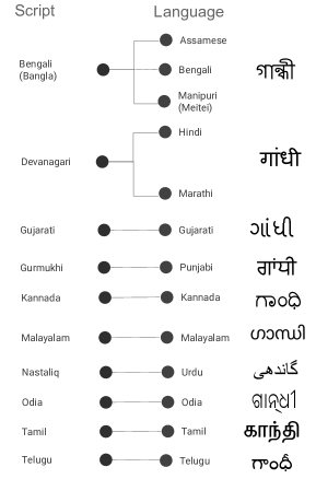
Figure 1. We study printed text recognition of 13 Indian languages (10 different scripts). Although these languages essentially use a common alphabet, script used to write these languages are different except for few languages that share common script such as Hindi and Marathi. In the last column we show how the name “Gandhi” is written in all the 10 scripts.

The challenges in text recognition varies based on the language/script the text is written in, how the text is rendered (handwritten, printed, or typewritten) and the way the document is imaged (scanned, captured using a mobile device, or born-digital). This work deals with recognition of text printed in Indian languages. Our focus is on text recognition alone. That is, we assume that cropped word or line images are provided. The 2011 official census of India (cen, [n. d.]) lists 30 Indian languages that have more than a million native speakers. 22 of them are granted official language status. These 22 languages belong to three different language families; Indo-European, Dravidian and Sino-Tibetan. Our work deals with text recognition in 13 of these 22 official languages of India. The languages are Assamese, Bangla, Gujarati, Hindi, Kannada, Malayalam, Manipuri, Marathi, Odia, Punjabi, Tamil, Telugu and Urdu. Many of these languages share common linguistic and grammatical structures. But script remain very different except for few languages. Among the 13 languages, Hindi and Marathi use Devanagari script and Bangla, Assamese and Manipuri use Bangla script.Others have their own unique scripts. Thus our study deals with printed text recognition of 13 Indian languages that use 10 different scripts Figure 1 shows how the name Gandhi is written in the 10 scripts. Though there have been many attempts in developing ocrs for Indian scripts from the 1970s to the beginning of this decade (Sinha and Mahabala, 1979; Chaudhuri and Pal, 1998; Arya et al., 2011), methods that can scale across languages and yield reasonable results over a wide variety of documents were not devised. Inherent challenges with the scripts and languages and lack of large-scale annotated data hindered the development of Indian language ocr for decades. Following the success of Connectionist Temporal Classification (CTC) for speech transcription, the same has been adapted for recognition of handwritten text (Graves et al., 2009), printed text (Thomas M. Breuel and Adnan Ul-Hasan and Mayce Ibrahim Ali Al Azawi and Faisal Shafait, 2013; Sankaran and Jawahar, 2012) and scene text (Su and Lu, 2014; Shi et al., 2015). Most popular open source OCR tools such as Tesseract (Tesseract developers, 2021), Easyocr (jaidedAI, 2022) and ocropy (ocropus, 2022) use a CTC based model for text recognition. The primary reasons for popularity of this approach is that word or line images can be recognized without the need for sub-word segmentation.

Segmenting a word into sub-word units is much more difficult for Indian languages compared to English (Sankaran and Jawahar, 2013). Another challenge in development of recognizers for Indian languages is the complex relationships between atomic units of the script (visual), language (text) and the machine representation. In a script, the atomic unit is an isolated symbol (a glyph), and from the language perspective atomic unit is an akshara or an orthographic syllable. And for the machine representation of text, atomic unit is a Unicode point. An akshara can be a combination of multiple glyphs in the script. Similarly an akshara is often represented by a sequence of multiple Unicodes. Akshara wise splitting of the text and mapping from akshraras to the corresponding Unicode sequence require knowledge of the language and script (Sankaran and Jawahar, 2013; Mathew et al., 2016). For these reasons, approaching text recognition as a sequence modelling problem using CTC has become the de-facto choice for OCR of Indian languages(Sankaran and Jawahar, 2013; Adnan Ul-Hasan and Saad Bin Ahmed and Sheikh Faisal Rashid and Faisal Shafait and Thomas M. Breuel, 2013; Krishnan et al., 2014). This approach can directly map a sequence of features from the word or line image to a target Unicode sequence, and an explicit alignment between feature sequence and the output Unicode sequence is not required during training. .

In this work we present a comprehensive empirical study of the the various design choices involved in building a CTC based printed text recognition model for Indian languages.

Our contributions are the following:

• For 13 Official languages of India, we empirically compare performance of four types of CTC-based text recognition that differ in terms of feature extraction and sequence encoding. We also compare word-level and line-level recognition models.

• Investigate the effectiveness of synthetic data as an alternative to training data, especially since lack of large-scale annotated data has always been a problem for Indian languages.

• Combining our best text recognition model for each language with existing line and word segmentation tools we build en-to-end page OCRs and compare their performance against Tesseract 5 and Google Cloud Vision OCR. Two of our page OCR pipelines perform better than the aforementioned OCR tools for 8 out of the 13 languages.

• We release a new public dataset for text recognition in 13 Indian languages. The dataset has cropped line segments and corresponding ground truth for 13 languages and cropped word segments and corresponding GT for all the 13 except Urdu. The dataset has more than 1.2 million annotated word images in total. To the best of our knowledge this is the largest dataset for text recognition in Indian languages.

2. Previous Works in Printed text recognition for Indian scripts

This section summarizes previous works related to printed text recognition for Indian scripts. We organize the section in three subsections, that reflect the evolutionary progress made in this space over the years.

2.1. First generation OCRs [1970 - 2000]

The first generation OCRs (Sinha and Mahabala, 1979; Chaudhuri and Pal, 1998) for Indian languages follow template matching style approach for character matching and use intuitive features such as shape and water reservoir. Pal and Chaudhuri (Pal and Chaudhuri, 2004) provides an excellent summary of methods developed in this period.

Sinha and Mahabala (Sinha and Mahabala, 1979) uses a syntactic pattern analysis system with an embedded picture language for recognition of Devanagari script. Here structural representations for each symbol of the Devanagari script is stored beforehand in terms of primitives and its relationships. The input word is digitized, cleaned, thinned ad segmented ( segmented to symbols) and labelled ( local feature extraction process). Recognition involves a search for primitives on the labelled pattern based on the stored description. Contextual constraints are also used to arrive at the correct recognition.

A complete ocr system for printed Bangla script is presented by Chaudhuri and Pal (Chaudhuri and Pal, 1998). In this work they use stroke based features to design a tree based classifier. These classifiers are used specifically to recognize compound characters. This is followed by a template matching approach to improve accuracy. The character unigram statistics is used to make the the tree classifier efficient. Several heuristics are also used to speed up the template matching approach. A dictionary-based error-correction scheme has been integrated where separate dictionaries are compiled for root word and suffixes that contain Morphy’s-syntactic information as well.

Antani and Agnihotri (S. Antanani and L. Agnihotri, 1999) created a dataset of Gujarati from scanned images and various sources in internet. They use invariant moments and raw (regular) moments as features. Image pixel values were used as features creating 600 dimensional binary feature space. For classification a K- Nearest Neighbour (k-nn) classifier along with a minimum hamming distance classifier is used. Negi et al. (Negi et al., 2001) use connected component analysis to extract isolated symbols from Telugu words. The segmented symbols are then matched against a stored template bank using fringe distance as the distance measure to perform the classification. Pal and Sarkar (U. Pal and A. Sarkar, 2003) propose a system to recognize Urdu script using a combination of topological, contour and water reservoir concept based features and a tree based classifier.

Lehal and Singh (G S Lehal and C Singh, 2000) developed a Gurumukhi script recognition system during the same period. They use connected component analysis to extract sub-word components from word images. They use two feature sets: primary features like number of junctions, number of loops, and their positions and secondary features like number of endpoints and their locations, nature of pro-files of different directions. A multistage classifications scheme is used by combining binary tree and nearest neighbour classifier. They supplement the recognizer with post-processor for Gurmukhi Script where statistical information of Panjabi language syllable combinations, corpora look-up and certain heuristics have been considered.

2.2. Second generation OCRs [2000 - 2012]

Second generation of OCRs started using more statistical, data driven features like Discrete Cosine Transform (DCT) and Principal Component Analysis (PCA) and Machine learning based approaches to classification like Support Vector Machines (SVM) and Artifical Neural Networks (ANN). A comparison and evaluation of state-of-the-art ocr systems developed during this period is presented in (Arya et al., 2011).

A Tamil and English bilingual text recognition system introduced by Aparna et al. (Aparna and Ramakrishnan, 2002) use geometric moments and dct coefficients to classify sub-word symbols. A nearest neighbour classifier with Euclidean distance as the distance measure is used.

Recognition of Kannada script using SVM has been proposed by Ashwin and Sastry (Ashwin and Sastry, 2002). To capture the shapes of the Kannada characters, they extract structural features that characterizes the distribution of foreground pixels in the radial and angular directions. In another work dealing with Kannada OCR, Kumar and Ramakrishnan (B. Vijay Kumar and A. G. Ramakrishnan, 2002) use coefficients of the DCT Discrete Wavelet Transform (DWT), and Karhunen-Louve Transform as features. Apart from the classic pattern classification technique of nearest neighbour, ANN based classifiers like Back Propagation and Radial Basis Function (RBF) Networks are studied. Kunte and Samuel (Sanjeev Kunte and Sudhaker Samuel, 2007) in a later work develop a Kannada ocr to recognize basic characters (vowels and consonants). Hu’s invariant moments and Zernike moments are used to extract the features of the characters. They use an RBF neural network as the classifier.

Jawahar et al. (C. V. Jawahar, MNSSK Pavan Kumar and S. S. Ravikiran, 2003) use PCA followed by an SVM classifier to classify Hindi and Telugu characters. Authors evaluate performance of the recognition process on approximately 200K characters for Hindi and Telugu and report a classification accuracy of 96.7%. Motivated by the success of Hidden Markov Models (HMMs) for continuous speech recognition, BBN BYBLOS OCR systems were introduced in the late 1990s (Makhoul et al., 1996; Lu et al., 1999). The HMM-based approach followed in BBN BYBLOS system does not require word or character level segmentation and training is language independent. Natarajan et al. (Natarajan et al., 2005) extended this approach to Devanagari. This work probably is the first approach to a segmentation free (without the need for sub-word segmentation) OCR of an Indian script. Ghosh et al. (Ghosh, Subhankar and Bora, P. K. and Das, Sanjib and Chaudhuri, B. B., 2012) modified an existing Bangla OCR model to recognize Assamese characters. Their model uses an SVM classifier followed by a spell checker. Rasagna et al. (Venkat Rasagna, Jinesh K.J. and C.V. Jawahar, 2011) develops a multi-font Telugu OCR using HOG features and SVM classifier. Experiments are conducted using a dataset that has more than 145 thousand Telugu character samples in 359 classes and 15 fonts. On this data set, authors report more than 96% character accuracy.

Neeba and Jawahar (N.V. and Jawahar, 2009) have performed an empirical evaluation of different character classification schemes. They study performance for a wide array of features such as moment based features and different types of classifiers. Classifiers studied in this work are nearest neighbour classifier, decision trees, Multilayer Perceptron ( MLP), Convolutional Neural Network (CNN) and SVM.

2.3. Third generation OCRs [2012 -]

Third generation OCRs for Indian scripts are primarily driven by segmentation free approaches that directly generate a sequence of labels given a word or line image. Sankaran et al. (Sankaran and Jawahar, 2012) were the first to adopt CTC based sequence modelling for the problem of printed text recognition of an Indian language. They use a Recurrent Neural Network (RNN) encoder and CTC transcription to map from a sequence of features extracted from a Devanagari word image (i.e., recognition unit is a word) to a sequence of class labels. Handcrafted profile-based features (Toni M. Rath and R. Manmatha, 2003) computed from A 25 x 1 sliding window are used as the features. The model uses aksharas as the output classes. Hence this model employs a rule based akshara to Unicode mapping. They extend this approach in (Sankaran and Jawahar, 2013) wherein feature sequence from the word image is directly mapped to the Unicode sequence avoiding the need for a rule based mapping from aksharas to Unicode. The CTC based transcription approach came as a boon for Indic scripts since sub-word segmentation has always been a challenge for most of the Indic scripts. In addition to it, transcribing the word image directly to machine readable form (Unicode sequence) avoided the need to write language specific rules to map from latent output classes (for example classes corresponding to the possible set of aksharas used in (Sankaran and Jawahar, 2012)) to a valid sequence of Unicodes.

Similar to the works discussed above, Hasan et al. (Adnan Ul-Hasan and Saad Bin Ahmed and Sheikh Faisal Rashid and Faisal Shafait and Thomas M. Breuel, 2013) use an RNN+CTC model to recognize printed text in Urdu. This work directly output Unicode sequence given an image of a text line (i.e., recognition unit is a line). Raw pixels extracted from a 30 x 1 sliding window manner forms the input feature sequence. Krishnan et al. (Krishnan et al., 2014) use profile based features and CTC-based model similar to the one in (Sankaran and Jawahar, 2013) fo recognition of 7 Indian langauges. They evaluate their approach on a test set comprising thousands of document images per language. The results demonstrate that a unified framework that uses CTC transcription works well for recognition of multiple Indian languages without the need for any language/script specific modules. Our own previous work (Mathew et al., 2016), proposes a two-step multilingual OCR system that can recognize text in 12 Indian languages and English (Mathew et al., 2016). A new dataset is presented in this work that has page level ground truth text annotations for 100 Hindi document images. We demonstrated that our CTC based OCR outperforms other free and commercial OCR solutions on the new dataset.

Chavan et al. (Chavan et al., 2017) conducts a comparative study by evaluating performance of an RNN and a multidimensional RNN (MDRNN) (Graves et al., 2007) encoders when used with CTC transcription. They use HOG (Histogram of Gradients) features with the RNN encoder and raw pixels for the MDRNN. This study concludes that MDRNN encoder performs better compared to the RNN encoder. An RNN+CTC transcription model is proposed for recognition of Bengali script in (Paul and Chaudhuri, 2019). This work reports 99%+ character/symbol accuracy for a test set that has word images rendered using more than 20+ fonts. Kundaikar and Pawar (Kundaikar and Pawar, 2020) study robustness of CTC based Devanagari OCR to font and font size variations. Dwivedi et al. (Dwivedi et al., 2020) use an encoder-decoder model for recognition of Sanskrit. The proposed solution achieve under 3% character/symbol error rate on a test set of Sanskrit line images that has much longer words compared to Latin or other Indian languages.

Most of the word or line based recognition models for Indian languages that we discuss above rely on CTC transcription. In this work we conduct a comprehensive empirical study of this approach for both line and word recognition by comparing different types of encoders and features.

3. Datasets

In this section, details of the datasets used in this study are presented. We use three datasets: i) an internal dataset that has nearly 1000 pages per language for the empirical study, ii) a new public dataset of cropped words and lines and the corresponding ground truth transcriptions, and iii) a dataset of synthetic word images for the experiments involving synthetic data.

3.1. Internal dataset

Language	Train				Test
	Books	Pages	Lines	Words	Books	Pages	Lines	Words
Assamese	14	901	23811	186471	5	98	3038	33636
Bangla	11	900	24490	199890	2	100	3120	26307
Gujarati	17	899	23591	186555	8	99	3141	32626
Hindi	27	899	23752	195111	6	101	2416	26131
Kannada	22	899	24270	184323	5	101	3448	17269
Malayalam	24	900	24383	183462	7	100	3054	14796
Manipuri	22	897	23466	183304	3	101	2890	25834
Marathi	17	898	23982	191496	3	102	3140	26709
Odia	14	898	24054	192494	3	102	2959	30582
Punjabi	24	899	23725	194900	8	101	2683	32158
Tamil	18	900	24129	181238	5	100	2869	14638
Telugu	24	899	23596	181083	4	101	2791	16748
Urdu	8	866	23250	-	1	93	1829	-

Table 1. Statistics of the internal dataset used in our study. This dataset has 1000 pages. Each page is annotated with word and line bounding boxes and the corresponding ground truth text transcriptions. For Urdu word level annotations are not available.

Our internal dataset comprises 1000 document images per language. The pages are taken from multiple books and scanned using a flatbed scanner. The pages are scanned in 300 in ppi for Assamese, Manipuri and Urdu and in 600 ppi for the rest. The pages mostly contain a single column of text arranged in paragraphs in simple layouts. For 12 out of the 13 languages, the pages are annotated with word and line bounding boxes and corresponding text transcription for the lines and words. For Urdu, only line level annotations are available. For each language the pages are split approximately in 80:10:10 ratio into train, validation and test splits. The splits are made in such a way that no two splits have pages from the same book. Statistics of the dataset is presented in Table 1

Language	Train		Validation		Test
	Lines	Words	Lines	Words	Lines	Words
Assamese	9566	79959	1196	9945	1196	10146
Bangla	7579	80113	948	9787	947	10113
Gujarati	8632	79910	1080	10016	1079	10090
Hindi	6525	79762	816	10114	816	10173
Kannada	13462	80085	1683	10088	1683	9838
Malayalam	15112	80146	1889	9893	1889	9980
Manipuri	9765	79691	1221	10254	1221	10061
Marathi	8380	80151	1048	10005	1048	9855
Odia	8260	79945	1033	10089	1033	9994
Punjabi	6726	79931	841	10036	841	10038
Tamil	16074	80022	2010	10021	2009	9974
Telugu	12722	80337	1591	9811	1590	9876
Urdu	9100	-	1138	-	1137	-

Table 2. Statistics of the new Mozhi dataset. It is a public dataset for printed text recognition of cropped words and lines. It has more than 1.2 million words annotated in total. For Urdu , only cropped lines are annotated.

3.2. Mozhi dataset

To the best of our knowledge, there are no large-scale public datasets for the problem of printed text recognition of Indian languages. Most of the early works in this space use a dataset of cropped characters or isolated symbols since these works deal with classification of disjoint characters (Sanjeev Kunte and Sudhaker Samuel, 2007; C. V. Jawahar, MNSSK Pavan Kumar and S. S. Ravikiran, 2003). Later works that make use of line or word level annotated data use either internal collections (Sankaran and Jawahar, 2012; Krishnan et al., 2014; Mathew et al., 2016; Chavan et al., 2017; Jain et al., 2017) or large-scale synthetically generated samples (Dwivedi et al., 2020; Kundaikar and Pawar, 2020; Adnan Ul-Hasan and Saad Bin Ahmed and Sheikh Faisal Rashid and Faisal Shafait and Thomas M. Breuel, 2013) to train their models. Some of the recent works including ours have introduced public datasets for Indian languages like Hindi and Urdu. They contain limited number of samples meant only for evaluation of the models (Mathew et al., 2016; Jain et al., 2017). Although these existing datasets serve as public benchmarks for evaluating different text recognition methods, training data used by these methods vary and hence a fair comparison of the methods is difficult.

In an attempt to address the scarcity of annotated data, to train printed text recognition models for Indian languages, we introduce a new public dataset named Mozhi (meaning “language” or “word” in Tamil and Malayalam) for all the 13 languages we study in this work. The dataset contains both line and word level annotations. For all the 13 languages, cropped line images and their corresponding ground truth text annotations are provided. Word images cropped from these text lines and the corresponding word level ground truths are also included for all languages except Urdu. The dataset has 1.2 million word annotations in total ( 100,000 per language), making it the largest ever public dataset of real word images, for text recognition in Indian languages. For each language, the line level data is split randomly in 80:10:10 ratio to train, validation and test splits respectively. Words that are cropped from line images in train split of lines forms the train split for words. Similarly for validation and test splits.

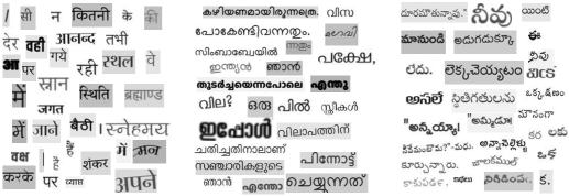
Figure 2. Samples of synthetic word images created for Hindi, Malayalam and Telugu.

3.3. Synthetic dataset

With the advent of deep learning based data driven methods, reliance on large-scale data to build machine learning models has only increased(Deng et al., 2009; Everingham et al., 2010; Krizhevsky et al., 2012). Deeper networks have more number of parameters and hence need large amounts of data to generalize well. Manually annotating data to train these models is often a tedious task. An alternative to using real training data is to generate synthetic training samples. Over the recent years this approach has successfully been used for many Computer Vision problems (Jaderberg et al., 2014; Rozantsev et al., 2015; Ros et al., 2016). Successful adaption of modern machine learning models for the problem of text recognition would not have been possible without large-scale synthetic datasets (Sankar et al., 2010; Rodríguez-Serrano et al., 2009; Jaderberg et al., 2014; Sabbour and Shafait, 2013; Mathew et al., 2017; Krishnan and Jawahar, 2016). Synthetic samples generated by font rendering have been used in many works including ours that deal with OCR of Indian languages. (Sabbour and Shafait, 2013; Adnan Ul-Hasan and Saad Bin Ahmed and Sheikh Faisal Rashid and Faisal Shafait and Thomas M. Breuel, 2013; Kundaikar and Pawar, 2020; Dwivedi et al., 2020; Mathew et al., 2017)

In this work, we investigate the effectiveness of synthetic data as an alternative to real data for training a text recognition model. To this end, we render synthetic word images for the same set of words that make up the train split of the internal dataset for the specific languag. We compare the performances when the recognition model is trained on real and synthetic datasets. We conduct this study for three languages — Hindi, Telugu and Malayalam. Freely available Unicode fonts are used to render the synthetic word images . The number of unique fonts used for Hindi, Malayalam and Telugu are are 97, 19, and 62 respectively. For rendering text onto images we use convert tool of ImageMagick (The ImageMagick Development Team, [n. d.]), Pango (Owen Taylor and Behdad Esfahbod, [n. d.]) and Cairo (Cairo developers, [n. d.]). In order to mimic the typical document images, we generate images whose background is always lighter (higher intensity) compared to the foreground. Each word is rendered as an image using a random font. Font size, font styling such as bold and italic, foreground and background intensities, kerning and skew are varied for each image to generate a diverse set of samples. A random one fourth of the images are smoothed using a Gausssian filter with a standard deviation($\sigma$) of 0.5. Finally, all the images are resized to a height of 32, while keeping the original aspect ratio. Samples from our synthetic dataset are shown in Figure 2 .

4. Text recognition using CTC transcription

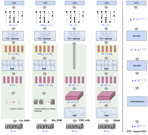
Figure 3. We study four CTC based text recognition approaches — Col_RNN, Win_RNN, CNN_only and CRNN, that differ in terms of the features extracted and the kind of sequence encoding used. $W$ and $H$ are width and height of the input image $I$ respectively. $|L^{\prime}|$ is the number of class labels including the blank label. $Hid_{j}$ denotes the number of hidden units in the last layer of the RNN. For the Win_RNN, $W_{W}$ and $S_{W}$ are width and step size of the sliding window respectively.

Given an input image $I$ of a word or a line, the task of text recognition aims to output the text present on the image in machine readable form. We model the task as a sequence modelling problem using CTC. Input is a sequence of features $\mathbf{x}=x_{1},x_{2},...,x_{T}$ where $x_{t}\in\mathbb{R}^{D}$ are extracted from the image $I$. Output is is a sequence of class labels $\mathbf{l}=l_{1},l_{2},...,l_{N}$, where $l_{n}\in{L}$, where $L$ is the output alphabet, i.e., the set of unique class labels. In our case, ${L}$ is the set of all Unicode code points that we are interested in recognizing.

For the below discussion, we use an encoder-decoder style interpretation of the CTC as given in (Hannun, 2017).

4.1. Extracting feature sequence

Graves et al. (Graves et al., 2006) first used CTC to transcribe speech to text. In their work, features are extracted , along the time axis of the speech signal, in a sliding window manner. They use a window of size 10 milli seconds (ms) and a step size of 5 ms. A feature vector of fixed size is extracted at each instance of the sliding window. Each individual unit of the input sequence are referred to as a ‘time-step’ or a ‘frame’. Unlike a 1D, time varying signal like speech, a grey-scale image is a 2D scalar valued spatial signal. Therefore, in order to form a 1D sequence of features, methods that use CTC to transcribe text from images, conventionally extract features along the horizontal axis of the image(Sankaran and Jawahar, 2013; Adnan Ul-Hasan and Saad Bin Ahmed and Sheikh Faisal Rashid and Faisal Shafait and Thomas M. Breuel, 2013; Shi et al., 2015). We follow the same approach. That is, feature vectors in the input sequence $\mathbf{x}$, correspond to a sequence of horizontal segments of the given image. Similar to the original work (Graves et al., 2006), an instance of the input sequence are referred to as a ‘time-step’ or a ‘frame’. The horizontal extent of a frame varies based on how the features are extracted. The feature sequence, $\mathbf{x}$ is extracted in the same direction as the script is written. That is, for all the languages except Urdu features are extracted from left to right, and for Urdu features are extracted in the opposite direction.

In summary given an image $I\in\mathbb{R}^{W\times H}$ (we work with grey scale images), a feature sequence is extracted as follows:

(1) $$\mathbf{x}\in\mathbb{R}^{T\times D}=FeatureExtract(I)$$

4.2. Encoder

The job of the sequence encoder is to take the input sequence $\mathbf{x}$ and map to encoded representation $\mathbf{x^{\prime}}\in\mathbb{R}^{T\times D^{\prime}}$ where $D^{\prime}$ is the encoding size; i.e., the fixed size to which each feature vector is encoded into.

i.e.,

(2) $$\mathbf{x^{\prime}}\in\mathbb{R}^{T\times D^{\prime}}=Encoder(\mathbf{x})$$

4.3. Feature and encoder configurations

Below we discuss 4 different types of feature and encoder combinations we study in this work.

Col_RNN: In this case , a frame of the input correspond to a single column of the image. Features are nothing but normalized pixel values (normalized in 0–1 range) of each column. This approach has been used in our previous works that deal with printed text recognition of Indian languages (Mathew et al., 2016; Krishnan et al., 2014). From the given image $I\in\mathbb{R}^{W\times H}$, feature sequence $\mathbf{x}\in\mathbb{R}^{W\times H}$ is extracted and a RNN is used to encode $\mathbf{x}$ to $\mathbf{x^{\prime}}\in\mathbb{R}^{W\times D^{\prime}}$ .

Win_RNN: Win_RNN uses an approach similar to the original work (Graves et al., 2006), to extract features in a sliding window manner. A sliding window of size $W_{w}\times H$ is moved across the image and at each step $t$, pixel values of the columns in the window are stacked to form the feature vector $x_{t}$. If the sliding window is moved with a step size $S_{w}$, then $\mathbf{x}$ will be of shape $\lfloor W/{S_{w}}\rfloor\times(H\cdot{W_{w}})$. Further $\mathbf{x}$ is encoded using a RNN to $\mathbf{x^{\prime}}\in\mathbb{R}^{\lfloor W/{S_{w}}\rfloor\times D^{\prime}}$. Col_RNN is in fact a Win_RNN with $W_{w}=S_{w}=1$.

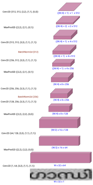
Figure 4. Architecture of the CNN used in CNN_only and CRNN configurations. This architecture is same as the one used in original CRNN paper (Shi et al., 2015). Written below the image or feature maps is the size in ${width}\times{height}\times{num.ofchannels}$ format. Conv2D, MaxPool2D and BatchNorm2D denote 2D convolution, 2D max pooling and 2d Batch Normalization operations respectively. The parameters for these operations are shown in the same format as the one used in PyTorch.

CNN_only: Unlike the above two approaches that uses pixel intensities as features, a CNN is used to extract features. Given an image $I$, CNN outputs a feature map $F\in\mathbb{R}^{W^{\prime}\times H^{\prime}\times C^{\prime}}$. $F$ is reshaped to $W^{\prime}\times(H^{\prime}\cdot C^{\prime})$ to form the sequence of features $\mathbf{x}$. In other words, from the feature map $F$, a sequence of $W^{\prime}$ feature vectors each of size $H^{\prime}\cdot C^{\prime}$ are formed. In this configuration, there is no dedicated sequence encoder. Or the encoder is an identity mapping. That is, in this configuration $\mathbf{x^{\prime}}=\mathbf{x}$.

CRNN: In this configuration, features are extracted using a CNN and an RNN is used to encode the sequence of features. This approach called ”CRNN”, was proposed by Shi et al. (Shi et al., 2015) for English scene text recognition. Similar to the CNN_only configuration, a CNN is used to obtain a feature sequence $\mathbf{x}\in W^{\prime}\times(H^{\prime}\cdot C^{\prime})$. $\mathbf{x}$ is then encoded using an RNN to form the final encoded sequence $\mathbf{x^{\prime}}\in\mathbb{R}^{W^{\prime}\times D^{\prime}}$.

All configurations we discuss above but CNN_only, use a RNN at the encoder and the size of the encoding $D^{\prime}$ depends on the number of units in the last recurrent layer. If a $J$ layer bi-directional RNN is used, then $D^{\prime}=2\cdot{Hid}_{J}$, where ${Hid}_{J}$ is the size of the hidden state of the last layer of the RNN.

The RNN encoder used in the above configurations is essentially encoding a 1D sequence of features. Or in other words, the RNN captures long term dependencies along the horizontal axis only. Graves et al. (Graves et al., 2007) proposed a multi-dimensional RNN (MDRNN) (Graves et al., 2007) that can model dependencies in more than one spatio-temporal dimensions. Although MDRNN has been proven successful for text recognition tasks (Alex Graves and Jürgen Schmidhuber, 2008), a later study by Puigcerver argued that computationally expensive MDRNNs are not essential for obtaining similar performances. He showed that the features extracted by MDRNN layers are visually similar to those extracted by a CNN. They further argue that two dimensional long term dependencies that are modelled by MDRNN layers may not be essential for the problem of text recognition. Motivated by the results of Puigcerver’s, study we do not experiment with MDRNNs in this work . Instead our CNN_only and CRNN configurations discussed above use convolutional layers to model dependencies along both dimensions of an image.

4.4. Decoder

The encoded features $\mathbf{x^{\prime}}$ are projected to the size equivalent to the number of the output classes using a linear projection layer followed by Softmax normalization. This step can be viewed as the decoding part of the CTC as interpreted in (Hannun, 2017). The original output alphabet $L$ is augmented by adding an extra label   for blank. That is, $L^{\prime}={L}\cup\sim$. Blank label corresponds to the the case when we want to assign no label for an input. The result of Softmax normalization at a time-step can be interpreted as class conditional probabilities at the time-step. Or in other words, Softmax yields the posterior distribution over the classes.

In summary. given the sequence of encoded features,

(3) $$\mathbf{y}\in\mathbb{R}^{T\times L^{\prime}}=Decoder(\mathbf{x^{\prime}})$$

where each $y_{t}\in R^{L^{\prime}}$ represent activations at time step $t$. Thus ${y}_{t}^{k}$ is a score indicating the probability of $k^{th}$ label at time step $t$.

4.5. Transcription using CTC

Objective of CTC transcription is to find the most probable sequence of class labels, given $\mathbf{y}$. Let ${L^{\prime}}^{T}$ be the set of sequences of length over the alphabet $L^{\prime}$. A element of ${L^{\prime}}^{T}$ is called a path and denoted by $\pi$. CTC makes an assumption that the target label sequence’s length is always shorter or equal to the length of the input sequence ($T$). This is the reason why we consider all length $T$ sequences over alphabet $L^{\prime}$.

If we assume that network prediction at a particular time step is independent of the predictions at other timesteps, probability of a path is the product of probabilities of individual labels in the path , at respective time steps. That is, Probability of a path $\pi$ , given input sequence $\mathbf{x}$ is

(4) $$p(\pi|x)=\prod_{t=1}^{T}y_{t}^{\pi^{t}}$$

where $y_{t}^{\pi^{t}}$ is the probability of $t$^th label of the path $\pi$.

A many to one, sequence to sequence mapping $\boldsymbol{\mathcal{B}}$ is defined from the set of all possible paths to the set of all possible labellings whose length is at most $T$ . i.e., $\boldsymbol{\mathcal{B}}:{L^{\prime}}^{T}\mapsto L^{\leq{T}}$. Note that the paths are defined over the augmented alphabet $L^{\prime}$ and the labellings are defined over the original alphabet $L$. $\boldsymbol{\mathcal{B}}$ maps a path $\pi$ to a labelling $\mathbf{l}$ by removing the blank labels and the repeated labels. For example the path “g$\sim\sim$aa$\sim$nd$\sim$hh$\sim\sim$ii” is mapped to the labelling “gandhi”.

Given an input feature sequence $\mathbf{x}$, the conditional probability of a labelling $\mathbf{l}$ is the sum of probabilities of all paths in ${L^{\prime}}^{T}$ that maps to $\mathbf{l}$. That is,

(5) $$p(\mathbf{l}|\mathbf{x})=\sum_{\pi\in{\boldsymbol{\mathcal{B}}^{-1}(\mathbf{l})}}p(\pi|\mathbf{x})$$

Explicitly computing the summation in Equation 5 is difficult since there are a large number of paths that map to a given labelling. Inspired by the forward-backward algorithm for HMMs (Rabiner, 1989), Graves et al. (Graves et al., 2006) proposed a dynamic programming algorithm for the efficient computation of Equation 5.

4.6. Training

Let the training dataset be $S=\{I_{i},\mathbf{l}_{i}\}$ where $I_{i}$ is a word or line image and and $\mathbf{l}_{i}$ is the corresponding ground truth labelling. The objective function for training the encoder-decoder neural network for CTC transcription is based on the principle of Maximum Likelihood. Minimizing the objective function must maximize the log likelihoods of the ground truth labelling. Therefore the objective function used is,

(6) $$\mathbb{O}=-\sum_{I_{i},\mathbf{l}_{i}\in S}\log p(\mathbf{l}_{i}|\mathbf{y}_{i})$$

where $y_{i}$ is the decoder output for the i^th sample. The above objective function can be optimized using gradient descent and backpropagation.

4.7. Inference

At the time of inference, given an input sequence $\mathbf{x}$, our CTC based classifier need to output the labelling $\mathbf{l}^{*}$ that has the highest probability as defined in Equation 5. Thus the CTC based classifier can be expressed a function $h(\mathbf{x}$, where

(7) $$h(\mathbf{x})=\underset{\mathbf{l}\in{L}^{\leq T}}{\arg\max}\,{p}(\mathbf{l}|\mathbf{x})$$

Similar to the HMMs, this step where the most probable labelling is found, is called decoding. But there is no tractable algorithm for finding the labelling $\mathbf{l}$ that maximizes $p(\mathbf{l}|\mathbf{x})$. Graves et al. (Graves et al., 2006) proposed two approximate methods instead — best path decoding and prefix search decoding. In this work we use the former. ‘Best path decoding’ as the name suggests output the labelling corresponding to the most probable path as the most probable sequence. i.e.,

(8) $$h(\mathbf{x})\approx\boldsymbol{\mathcal{B}}(\pi^{*})$$

where $\pi^{*}$ is a path formed by concatenating the most probable labels in each time step. Note that best path decoding is an approximation and there is no guarantee that it will always yield the most probable labelling.

5. Experimental setup

Details of the steps taken to pre-process the data, hyper parameters of the encoder and decoder and specifics of the network training are presented in this section. We also summarize the evaluation metrics we use to evaluate the text recognition performance in both recognition-only and end-to-end settings.

5.1. Implementation details

In all experiments, input images of cropped words or lines are converted to grey scale and resized to a height of 32 pixels while keeping the original aspect ratio. There is no separate validation split for the internal dataset. Therefore, for all languages, we form a validation split by taking random 5% pages from each of the books in the train split. Thus validation split of the internal dataset has pages similar to the pages in train split, and the test split has pages from a different set of books.

While training our models on word or line samples from the internal dataset, the output alphabet $L$ for a language is the set of unique Unicode points found in the respective train split for that language. Similarly, while working with Mozhi dataset, the output alphabet for a language is the set of Unicode points in the train split for that language in the Mozhi dataset. For any language, the alphabet used for the line recognition model will have only one extra label — the label corresponding to white space — compared to the alphabet used for word recognition model of the same language. Word images in synthetic dataset for a language (see subsection 3.3) are rendered using the same set of words in the train split for that language in the internal dataset. Therefore the output alphabet used while training on synthetic data for a language is same as the alphabet used for the language while training on internal dataset.

For Win_RNN, the sliding window width $W_{W}$ is $20$ and step size $W_{S}$ is $5$. The RNN we use in Col_RNN, Win_RNN and CRNN has number of layers $J=2$. We use a bi-directional LSTM with 256 hidden units per direction, in each layer. Therefore the size of output of the RNN, at a time step is $2$ times $256$. The CNN block in CNN_only and CRNN models has the exact same architecture as in the original CRNN paper (Shi et al., 2015). The full architecture of the CNN is shown in Figure 4. Our models are implemented in PyTorch (Paszke et al., 2019). We build on an existing third party implementation of CRNN architecture (Holmeyoung, 2019). All our models are trained on a single Nvidia GeForce 1080 Ti GPU. While training on the internal dataset, we train all the models for 15 epochs and the CRNN models trained on the Mozhi dataset are trained for 30 epochs. A batch size of 64 and 16 is used for word and line recognition models respectively. We use RMSProp (Hinton, 2012) as the optimizer. For Col_RNN and Win_RNN a learning rate of $10e-03$ is used. For CNN_only and CRNN variants a slower learning rate of $10e-04$ was found to be better for faster convergence. The checkpoint that yields the highest Character Accuracy (refer subsection 5.2) on the respective validation data is saved for evaluation on test split.

5.2. Evaluation

We require to evaluate text recognition in three scenarios, i) word OCR : recognition of a cropped word image, ii ) line OCR: recognition of a cropped line image and iii) page OCR: end-to-end text recognition where input is a document image. In all the three cases, our primary evaluation metric is Character Accuracy (CA), which is based on Levenshtein distance between predicted and ground truth strings.

For a formal definition of CA, let us denote the predicted text for a word/line/page as $l_{i}$ and the corresponding ground truth as $g_{i}$. If there are $N$ such samples, CA is defined as

(9) $$CA=\frac{\sum_{i}len(g_{i})-\sum_{i}LD(l_{i},g_{i})}{\sum_{i}len(g_{i})}\times 100$$

where $len$ is a function that returns the length of the given string and $LD$ is a function that computes the Levenshtein distance between the given pair of strings. Note that Character Error Rate (CER) which is another commonly used metric for OCR evaluation is essentially $100-CA$.

For word OCR and line OCR, in addition to CA, we report Sequence Accuracy (SA). It is the percentage of samples for which the prediction is fully correct (i.e. $LD(l_{i},g_{i})=0$). In case of a word recognition model SA is same as ‘word accuracy’ or ’accuracy’ as used in scene text recognition literature.

For page OCR, where input is a document image, we use a standard OCR evaluation toolkit. A modern port (Santos, 2019) of the original ISRI Analytic Tools for OCR Evaluation (Rice and Nartker, 1996) is used. Using the ISRI toolkit, we report Character Accuracy (CA) and Word Accuracy (WA). In ISRI toolkit, CA is computed in the same manner as given in Equation 9. Word accuracy is computed by aligning the sequence of words in the prediction $l_{i}$ and sequence of words in ground truth $g_{i}$, and finding the Longest Common Sub-sequence (LCS) of the two. For a set of pages,

(10) $$WA=\frac{\sum_{i}{len(LCS(l_{i},g_{i}))}}{\sum_{i}len(g_{i})}\times 100$$

where $len$ returns the number of words in a given sequence of words.

6. Experiments and Results

In this section we present the details of the experiments we conduct and report and discuss the results.

6.1. Comparing different feature + encoder configurations

Language	Word								Line
	Col_RNN		Win_RNN		CNN_only		CRNN		Col_RNN		Win_RNN		CNN_only		CRNN
	CA	SA	CA	SA	CA	SA	CA	SA	CA	SA	CA	SA	CA	SA	CA	SA
Assamese	98.6	95.4	97.6	92.9	98.3	96.0	99.0	96.5	99.1	78.8	98.1	65.5	99.0	73.8	99.2	80.8
Bangla	99.1	97.0	98.3	94.5	99.2	97.3	99.4	97.9	99.1	73.7	98.4	59.6	99.2	73.9	99.4	79.7
Guajrati	96.2	92.4	95.1	89.5	96.2	90.9	96.5	93.9	96.5	66.3	94.6	49.9	96.0	62.2	96.9	67.4
Hindi	97.6	95.1	96.3	92.3	97.4	94.2	98.2	96.3	98.8	64.9	97.8	48.8	98.8	64.3	98.9	66.9
Kannada	97.4	88.9	96.4	84.7	96.7	85.8	97.7	90.7	97.4	49.2	96.4	38.2	97.0	42.9	97.5	49.4
Malayalam	99.5	96.6	99.3	95.6	98.0	83.7	99.7	97.7	99.5	84.8	99.3	80.5	98.5	49.7	99.7	86.9
Manipuri	98.6	95.4	97.8	92.8	98.2	93.1	99.0	96.9	99.4	79.9	98.7	67.6	99.4	79.2	99.5	80.9
Marathi	99.0	96.2	98.5	94.2	98.9	95.0	99.2	96.9	99.1	71.2	98.4	55.0	99.0	67.1	99.1	71.7
Odia	96.8	93.5	95.7	90.8	96.9	93.7	97.2	94.8	97.9	73.9	96.8	60.2	97.9	70.5	98.1	74.2
Punjabi	99.1	97.7	98.4	96.4	99.2	97.8	99.5	98.7	99.1	76.6	98.3	62.5	99.2	78.7	99.3	79.9
Tamil	97.9	91.0	97.4	88.4	97.3	87.2	98.0	91.8	96.3	43.8	95.9	40.7	96.2	41.2	96.5	45.0
Telugu	96.3	91.4	95.3	86.8	96.4	92.0	96.8	93.6	96.5	68.9	95.2	50.5	96.7	68.4	97.0	75.0
Urdu	-	-	-	-	-	-	-	-	93.9	23.2	75.8	4.2	91.9	17.0	93.5	24.1

Table 3. Recognition-only results on the validation splits of internal dataset. The left half shows results when recognition unit is a word (word OCR) and the other half shows results of the line OCR setting. Note that we train a separate model for each language in each setting. In both settings, we report Character Accuracy (CA) and Sequence Accuracy (SA) for all the four model configurations. The numbers shown in bold are the best CA and SA among the four feature + encoder configurations.

’

Language	Word		Line
	CA	SA	CA	SA
Assamese	99.1	96.9	99.4	73.3
Bangla	98.9	96.7	98.7	75.4
Guajrati	97.2	93.0	97.5	53.1
Hindi	97.4	94.0	98.0	51.2
Kannada	94.2	86.5	93.7	49.8
Malayalam	99.3	94.8	99.3	77.7
Manipuri	98.1	93.7	98.7	63.2
Marathi	99.6	97.9	99.5	81.7
Odia	97.8	94.8	98.0	61.4
Punjabi	99.0	97.8	99.2	78.8
Tamil	95.4	84.5	95.9	41.2
Telugu	99.0	94.7	98.9	69.4
Urdu	-	-	93.5	7.5

Table 4. Recognition-only performance using CRNN on the test splits of internal dataset. Here we use the CRNN checkpoint that yielded the highest CA on validation split.

We evaluate performance of the 4 different feature + encoder configurations (see subsection 4.3) on the internal dataset for word and line recognition performance. Results of this experiment are shown in Table 3. Models are trained on the train split and evaluated on the validation split of the respective language.

Note that each CA and SA pair in Table 3 correspond to a CTC-based network that was trained separately for a certain combination of language, recognition unit (line or word) and feature + encoder configuration (Col_RNN, Win_RNN, CNN_only or CRNN). In all cases except for Urdu line recognition, CRNN performs the best among 4 configurations. CRNN performing better than Col_RNN and Win_RNN substantiate the superiority of features learnt using a CNN compared to handcrafted features like normalized pixel values.

Similarly, improved performance for CRNN compared to CNN_only configuration validates the need for modelling long term dependencies. Unlike fully connected networks, neurons in successive layers in a CNN ‘sees’ only a local region of the input feature map. In order to build a CNN, where a neuron in the last layer has receptive filed covering the entire input, we need to stack a large number convolutional layers. The 7 layer CNN we use is not deep enough to model long term dependencies along the horizontal axis. Thi is compensated by the use of a sequence encoder (a bi-directional LSTM) that efficiently models long term dependencies in both directions, along the horizontal axis of the input.

Since CRNN works the best except for Urdu line level recognition, we only evaluate the CRNN configuration on the test set. These results are reported in Table 4. The Col_RNN configuration that performs the best for Urdu line recognition on the validation split, yields a CA of 92.0 and SA of 3.6 Urdu test split.

6.2. Page OCR evaluation on the Internal dataset

Language	End-to-end OCR tools				GT detection + our CRNN				Automatic detection + our CRNN
	Tesseract		Google		GT word		GT line		Tesseract word		Tesseract line		Google word		Google line		Scale space line
	CA	SA	CA	SA	CA	SA	CA	SA	CA	SA	CA	SA	CA	SA	CA	SA	CA	SA
Assamese	92.7	91.2	90.0	86.0	99.3	97.0	99.4	97.2	94.4	94.5	96.8	94.5	94.6	92.0	98.7	95.7	98.6	96.5
Bangla	93.5	96.2	84.0	91.3	99.1	97.3	99.0	96.8	97.7	96.2	98.6	96.3	91.8	92.0	96.3	92.5	96.4	94.9
Gujarati	96.9	92.4	93.0	95.2	98.0	93.7	97.7	91.9	91.7	81.9	93.6	88.4	88.6	74.3	93.1	79.6	75.2	67.7
Hindi	95.0	93.3	95.2	97.3	98.1	96.0	98.0	95.6	94.6	91.5	95.5	93.2	92.4	87.6	95.7	92.3	96.1	93.7
Kannada	94.9	85.1	85.7	84.6	95.6	89.2	95.9	86.4	70.0	61.1	70.6	62.1	72.5	63.9	72.2	64.2	67.2	64.6
Malayalam	96.2	78.7	88.0	74.8	99.4	98.0	99.3	97.9	98.1	91.6	98.8	96.7	96.3	83.2	97.7	91.9	98.2	96.3
Manipuri	90.9	80.6	85.7	77.4	98.4	94.7	98.7	94.9	95.9	89.2	97.4	93.7	86.9	64.0	96.4	87.5	98.0	93.8
Marathi	97.9	97.4	98.3	98.4	99.6	98.2	99.5	98.0	96.3	96.1	97.2	96.2	97.4	93.2	98.1	95.6	86.5	82.9
Odia	94.0	83.6	92.6	90.0	98.6	95.4	98.0	94.5	95.4	89.2	96.9	93.3	86.6	67.1	96.0	89.5	98.3	94.8
Punajbi	93.2	89.8	92.7	96.7	99.2	98.3	99.3	97.9	94.7	91.6	96.0	95.1	91.5	85.0	97.6	95.3	96.5	95.7
Tamil	79.3	42.4	92.5	93.1	96.1	85.6	96.5	85.4	92.4	80.0	93.6	83.4	88.0	60.6	93.7	79.1	93.3	82.0
Telugu	93.7	79.3	94.2	89.2	99.1	95.1	98.9	94.0	89.3	83.2	89.2	83.5	91.4	71.9	96.3	86.0	83.8	79.9
Urdu	68.3	26.2	92.7	85.7	-	-	94.7	81.5	-	-	88.9	74.4	-	-	90.0	68.8	56.4	45.5

Table 5. Performance of our page OCR pipelines compared to other public OCR tools. In this setting we evaluate text recognition in end-to-end manner on the test split of the internal dataset. Since the focus of this work is on text recognition, for end-to-end setting, for text detection, either gold standard word/line bounding boxes or automatic text detection tools are used. Under ‘End-to-end OCR tools’ we show results of Tesseract (Tesseract developers, 2021) and Google Cloud Vision OCR (Google, 2021a). Given a document image these tools output a transcription of the page along with the bounding boxes of the lines and words detected. Under ‘GT detection + our CRNN’ we show results of end-to-end pipeline where gold standard word and line detections are used. For instance, ’GT Word’ means we used ground truth (GT) word bounding boxes and the CRNN model trained for recognizing words, for that particular language. Under ‘Automatic detection + our CRNN’ we show results of the following end-to-end pipelines: i) Tesseract word detections + our CRNN word model, ii) Tesseract line detections + our CRNN line model, iii) Google OCR word detections + our CRNN word model, iv) Google OCR line detections + our CRNN line model and v) Scale space (Manmatha and Srimal, 1999) line detections + our CRNN line model.

In page OCR setting, input to the OCR is a document image and the expected output is the transcription of the textual content in the image. For a page OCR, typical approach is to use a page segmentation step that detects lines or words followed by a word or line level text recognition model. Finally, text transcriptions for individual lines or words are combined to form a page level transcription. In a typical scenario, end-to-end OCR involves layout analysis to identify different document layout objects and techniques to identify the reading order. This work’s focus is on text recognition (i.e., recognize text present in a given word or line image). Detecting words or lines on document images is beyond the scope of this work. Therefore we build end-to-end page OCR pipeline where text detection is done using existing method(s) or tool(s) and recognition of words or lines is done using our CRNN models. Once we have transcriptions for individual words or lines, we concatenate them in the same reading order as found by the page segmentation tool. In order to assess the upper bound on the end-to-end text recognition performance of our CRNN model, we evaluate an end-to-end pipeline where gold standard line or word detections are used. We further compare results of our end-to-end OCR with two publicly available OCR tools.

We use two public OCR tools. Tesseract (Tesseract developers, 2021) and Google cloud vision OCR (Google, 2021a). The former is an open-source OCR while the latter is a commercial, cloud-based solution. Tesseract version $5.1.4$ is used. We used page segmentation mode (psm) 3 of Tesseract that does automatic page segmentation but without automatic script detection. We used trained models provided in the official Tesseract repository (Google, 2021b). For Manipuri, since there is no trained models available, we used the model trained for Bengali. With the Google cloud vision we use the DOCUMENT_TEXT_DETECTION feature that is specifically designed for document images. At the time we used Google cloud vision OCR, Manipuri was not supported and Urdu and Odia OCRs were in experimental stage. From the results we could see that, automatic language detection of the DOCUMENT_TEXT_DETECTION identified most of the Manipuri text blocks as either Bengali or Assamese.

While building end-to-end pipelines that uses our recognition model with automatic text detection, we try out text detections from from the following: i) line and word detections from Tesseract, ii) line and word detections from Google cloud vision OCR and iii) line detections using scale space method proposed by Manmatha et al. (Manmatha and Srimal, 1999), The Tesseract and Google OCR that we use for text detections here is exactly same as the ones we use for end-to-end OCR (see the previous paragraph). Along with the text transcriptions these tools provide the bounding boxes of lines and words that were detected. These detections are used with our recognition model to build an end-to-end OCR. For the scale space approach, we use a third-party implementation (Scheidl, 2021). We use the text lines detected by this method and the text on these line segments are recognized using the line level CRNN model trained on the internal dataset for the respective language. We found the word detections using this method is highly noisy with many under segmentation cases. Hence we do not try out an end-to-end pipeline that use word detections from the scale space method. We set the parameters for the scale space algorithm as instructed in (Scheidl, 2021). We use different parameter values for document images in different languages. Values of the parameters are determined based on the average height and aspect ratio of the text lines in the train split. This approach simply sorts the detections in the default reading order. The default order may not be correct in case of complex layouts and multi column text. Since most document images in our internal dataset contain single column text without any non text elements, using default reading order is sufficient in most cases.

Results of all the end-to-end evaluations are reported in Table 5.

Model	Trained on	Fine tuned on	Hindi		Malayalam		Telugu
			CA	SA	CA	SA	CA	SA
real-only	real	NA	97.4	94.0	99.3	94.8	99.0	94.7
synth-only	synthetic	NA	93.3($\Downarrow 4.2\%$)	84.9($\Downarrow 9.7\%$)	98.2($\Downarrow 1.1\%$)	88.4($\Downarrow 6.7\%$)	95.5($\Downarrow 3.5\%$)	80.0($\Downarrow 15.5\%$)
synth + 0.1 real	synthetic	10% real	96.9($\Downarrow 0.5\%$)	92.8($\Downarrow 1.2\%$)	99.2($\Downarrow 0.1\%$)	94.2($\Downarrow 0.6\%$)	98.7($\Downarrow 0.3\%$)	93.1($\Downarrow 1.6\%$)
synth + 0.5 real	synthetic	50% real	97.4($\Updownarrow 0.0\%$)	94.0($\Updownarrow 0.0\%$)	99.3($\Updownarrow 0.0\%$)	94.7($\Downarrow 0.1\%$)	99.0($\Updownarrow 0.0\%$)	94.7($\Updownarrow 0.0\%$)

Table 6. Synthetic to real transfer learning Results.. ‘real-only’ and ‘synth-only’ are models trained exclusively on real and synthetic samples respectively. We fine tune the synth-only models using varying amounts of real data. synth + 0.1 real is the case when the synth-only model is fine tuned with a random $10\%$ of the real samples. Similarly synth + 0.5 real is a model where the synth-only model is fine tuned with half of the real training data. The values shown in brackets next to accuracy values are relative gain or drop in accuracy compared to the corresponding accuracy for real-only model. $\Downarrow$ indicate drop in accuracy and $\Updownarrow$ is used when there is no change in accuracy. For all languages, synth-only model can be fine tuned for performance on par with the real-only model by fine-tuning the real-only model on half of the real training data.

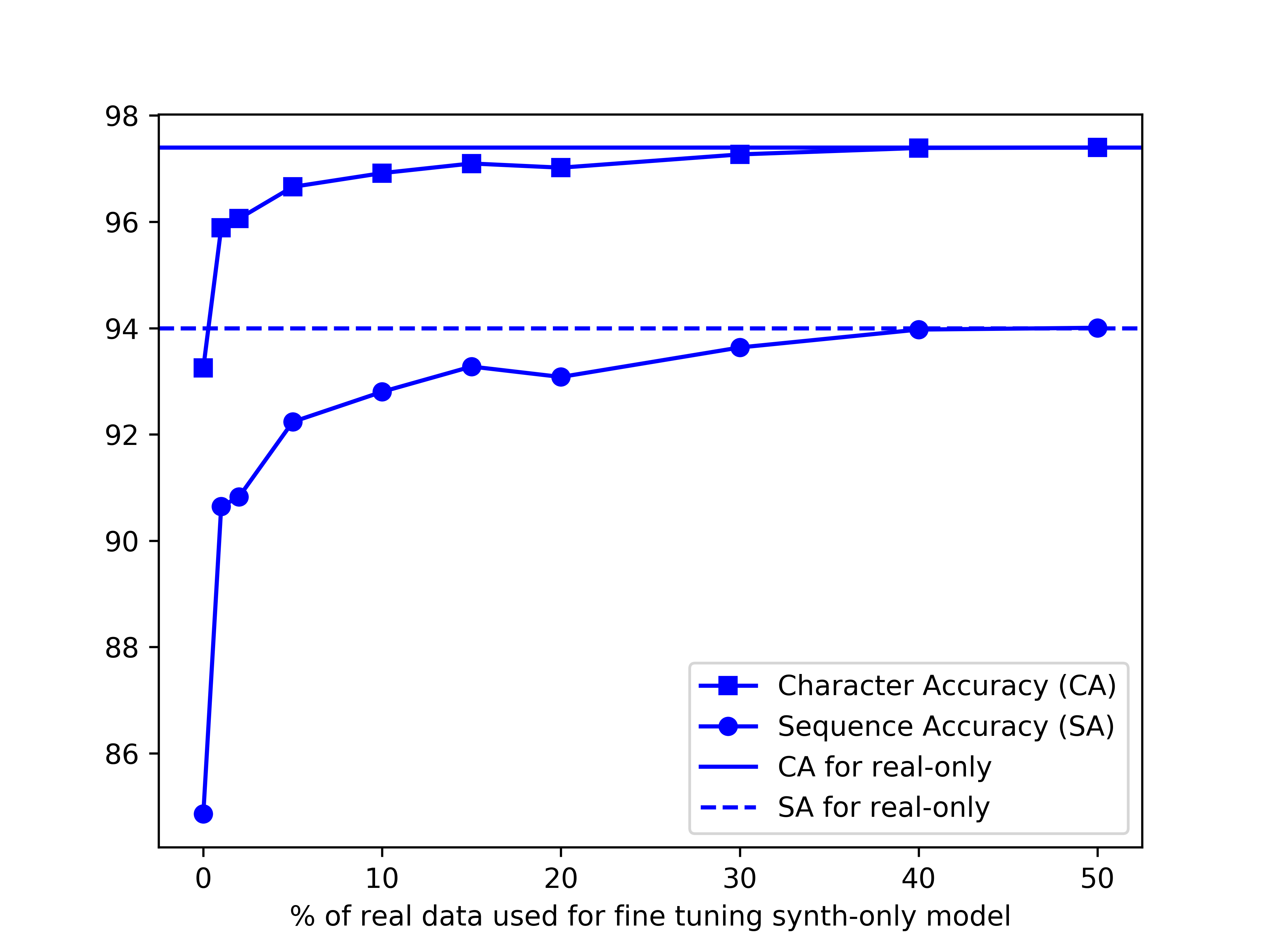
Figure 5. Transfer learning from real to synth by finetuning the synth-only model. The plot shown above is for Hindi. The model that uses $0\%$ real data for fine tuning is the synth-only model that is trained purely on synthetic data. This model is then fine tuned with real data, that is randomly sampled from the train split of the internal dataset. With finetuning on just $1\%$ of the real data, the CA jumps from 93.3 to 95.9 and the SA jumps from 84.9 to 90.6. With 40% or more real data, performance gain from the finetuning starts saturating and matches performance of the real-only model

6.3. Transfer learning from synthetic to real

In this section we report results of our experiments involving synthetically trained word samples. We investigate the effectiveness of synthetic data for training word recognition models. Results of these experiments are reported in Table 6. For three languages—Hindi, Malayalam and Telugu—we train word level CRNN models, on the respective synthetic datasets (see  subsection 3.3). These models are called ’synth-only’ since they are trained purely on synthetic data. The validation data used for these experiments is same as the validation data used for the respective languages for training word level models on the internal dataset. The model checkpoint that yields the best CA on the validation data is saved for evaluation on the test split. We evaluate these models on real samples in the test split for the respective language in the internal dataset. In Table 6 a ’real-only’ model for a language is a CRNN model that is trained on the word samples in the train split of the internal dataset for the language. Thus the results of real-only models we report in  Table 6 are same as the numbers we report for the three languages for word-level CRNN on validation and test splits in Table 3 and Table 4 respectively. As expected, For all languages, the synth-only has lower performance than real-only model. But the drop in performance is not large. The relative drop in CA, compared to the corresponding real-only model is not more than $5\%$ for any language. With finetuning on only 10% of the real data, the synth-only models reach CA levels comparable to that of the real-only models. And with finetuning on $50\%$ of the real data, the CA is same as that of the real-only models for all languages. The SA (or the word accuracy since these are word recognition models) for synth + 0.5 real is same as the SA for real-only models for Hindi and Telugu. In Figure 1 we show how increasing the amount of real data used for fine tuning improves the performance of the synth-only model for Hindi. Both CA and SA saturate and matches the performance of the real-only model with $40\%$ of the real data.

We conduct transfer learning experiments where we fine tune the synth-only models using real data. The results of these experiments are shown in the last two rows of Table 6. ‘synth + 0.1 real’ is the model where we fine tune the synth-only model using a random $10\%$ of the real word samples from the internal dataset. Similarly synth + 0.5 real is fine tuned with half of the samples in the real word samples that are randomly sampled from the train split of the internal dataset.

6.4. Evaluating CRNN on Mozhi dataset

The results of word and line recognition on the new Mozhi benchmark dataset using CRNN are reported in Table 7. For a language, for both word and line, we train a CRNN from scratch on the respective train split of the Mozhi dataset.

The numbers reported for the validation set are the best CA we obtain and the SA we get using the same checkpoint. We then evaluate the same checkpoint on the Test split.

Language	Validation				Test
	Word		Line		Word		Line
	CA	SA	CA	SA	CA	SA	CA	SA
Assamese	98.0	95.1	98.7	76.9	98.9	96.2	99.2	76.8
Bangla	99.2	97.0	98.4	69.5	99.0	96.9	98.1	68.4
Guajrati	98.3	95.3	97.8	61.4	98.0	94.9	97.4	63.1
Hindi	98.2	95.9	98.8	61.8	98.1	95.5	98.8	63.5
Kannada	96.6	88.4	97.1	53.2	97.1	88.7	97.5	53.9
Malayalam	99.6	97.2	99.5	86.0	99.5	97.3	99.5	87.3
Manipuri	98.4	95.8	99.1	80.3	98.4	95.9	99.2	79.4
Marathi	99.2	96.7	99.2	73.5	99.3	97.0	99.3	73.8
Odia	98.1	85.2	98.9	74.4	97.5	94.3	98.8	73.1
Punjabi	99.4	98.6	99.4	81.9	99.2	98.2	99.3	79.7
Tamil	98.2	92.0	98.5	70.1	98.0	91.6	98.3	68.1
Telugu	99.2	96.1	98.9	74.2	99.1	95.4	98.9	71.7
Urdu	-	-	93.6	26.5	-	-	93.8	24.2

Table 7. CRNN evaluation on Mozhi dataset.. For each language train both word and line level CRNN models on the respective train split of the Mozhi dataset. The models are trained from scratch. We use neither internal not synthetic data to train these models.

7. Conclusion

We conduct an empirical study of different CTC-based based models for word and line recognition, for 13 Indian languages. Our study concludes that CRNN, that uses a CNN for feature representation and a dedicated RNN-based sequential encoder works the best. Using existing text detection tools and our recognition models, we build page OCR pipelines and show that our approach works better than two popular OCR tools for most of the languages. We create font rendered synthetic word image samples and train word recognition models for 3 languages. We conduct a transfer learning experiment where we analyze how the performance of models trained purely on synthetic data improves, when fine-tuned on real data. Our results show that models pretrained on synthetic data and then fine tuned with half of the real training data perform equally well as the models trained on whole of the real data. The results suggests that, font rendered synthetic samples is a good alternative to real data to train text recognition models for low resource languages. We also introduce a new public dataset for cropped word/line recognition in 13 Indian languages, that has more than 1.2 million annotated words in total. We believe our our study and the Mozhi dataset will encourage research on OCR of Indian languages.

- (1)
- abb ([n. d.]) [n. d.]. ABBYY FineReader. http://www.abbyy.com/
- cen ([n. d.]) [n. d.]. Census 2011. https://censusindia.gov.in/2011-Common/CensusData2011.Html.
- ocr ([n. d.]) [n. d.]. The OCRopus(tm) open source document analysis and OCR system. http://code.google.com/p/ocropus/
- Adnan Ul-Hasan and Saad Bin Ahmed and Sheikh Faisal Rashid and Faisal Shafait and Thomas M. Breuel (2013) Adnan Ul-Hasan and Saad Bin Ahmed and Sheikh Faisal Rashid and Faisal Shafait and Thomas M. Breuel. 2013. Offline Printed Urdu Nastaleeq Script Recognition with Bidirectional LSTM Networks. In ICDAR.
- Alex Graves and Jürgen Schmidhuber (2008) Alex Graves and Jürgen Schmidhuber. 2008. Offline Handwriting Recognition with Multidimensional Recurrent Neural Networks. In NIPS.
- Aparna and Ramakrishnan (2002) K.G Aparna and A.G. Ramakrishnan. 2002. A complete Tamil Optical Character Recognition System. In Document Analysis System.
- Arya et al. (2011) Deepak Arya, Tushar Patnaik, Santanu Chaudhury, C V Jawahar, B.B.Chaudhuri, A.G.Ramakrishna, Chakravarty Bhagvati, and G. S. Lehal. 2011. Experiences of Integration and Performance Testing of Multilingual OCR for Printed Indian Scripts. In J-MOCR Workshop,ICDAR .
- Ashwin and Sastry (2002) T.V Ashwin and P. S. Sastry. 2002. A font and size independent OCR system for printed Kannada documents using Support Machines. Sadhana (2002).
- B. Vijay Kumar and A. G. Ramakrishnan (2002) B. Vijay Kumar and A. G. Ramakrishnan. 2002. Machine Recognition of Printed Kannada Text. In Document Analysis Systems V.
- C. V. Jawahar, MNSSK Pavan Kumar and S. S. Ravikiran (2003) C. V. Jawahar, MNSSK Pavan Kumar and S. S. Ravikiran. 2003. A Bilingual OCR system for Hindi-Telugu Documents and its Applications. In International Conference on Document Analysis and Recognition(ICDAR).
- Cairo developers ([n. d.]) Cairo developers. [n. d.]. Cairo. https://www.cairographics.org/
- Chaudhuri and Pal (1998) Bidyut Baran Chaudhuri and U. Pal. 1998. A complete printed Bangla OCR system. Pattern Recognition 31 (1998), 531–549.
- Chavan et al. (2017) Vishal Chavan, Abhijit Malage, Kapil Mehrotra, and Manish Kumar Gupta. 2017. Printed text recognition using BLSTM and MDLSTM for Indian languages. In International Conference on Image Information Processing (ICIIP).
- Deng et al. (2009) J. Deng, W. Dong, R. Socher, L.-J. Li, K. Li, and L. Fei-Fei. 2009. ImageNet: A Large-Scale Hierarchical Image Database. In CVPR09.
- developers ([n. d.]) Tesseract developers. [n. d.]. Tesseract OCR. https://opensource.google.com/projects/tesseract. Accessed on 10 November 2021.
- Dwivedi et al. (2020) Agam Dwivedi, Rohit Saluja, and Ravi Kiran Sarvadevabhatla. 2020. An OCR for Classical Indic Documents Containing Arbitrarily Long Words. In CVPR Workshops.
- Everingham et al. (2010) M. Everingham, L. Van Gool, C. K. I. Williams, J. Winn, and A. Zisserman. 2010. The Pascal Visual Object Classes (VOC) Challenge. International Journal of Computer Vision (2010).
- G Nagy (1992) G Nagy. 1992. At the frontiers of OCR. In Proceedings of IEEE.
- G S Lehal and C Singh (2000) G S Lehal and C Singh. 2000. A Gurumukhi Script Recognition System. In Inernational Conference on Pattern Recognition (ICPR).
- Ghosh, Subhankar and Bora, P. K. and Das, Sanjib and Chaudhuri, B. B. (2012) Ghosh, Subhankar and Bora, P. K. and Das, Sanjib and Chaudhuri, B. B. 2012. Development of an Assamese OCR Using Bangla OCR. In Proceeding of the Workshop on Document Analysis and Recognition.
- Google (2021a) Google. 2021a. Google Cloud Vision OCR. https://cloud.google.com/vision/docs/ocr. Accessed on 10 November 2021.
- Google (2021b) Google. 2021b. tessdata. https://github.com/tesseract-ocr/tessdata. Accessed on 10 November 2021.
- Graves et al. (2006) Alex Graves, Santiago Fernández, Faustino J. Gomez, and Jürgen Schmidhuber. 2006. Connectionist temporal classification: labelling unsegmented sequence data with recurrent neural networks. In ICML.
- Graves et al. (2007) Alex Graves, Santiago Fernández, and Jürgen Schmidhuber. 2007. Multi-dimensional Recurrent Neural Networks. In ICANN.
- Graves et al. (2009) Alex Graves, Marcus Liwicki, S. Fernandez, Roman Bertolami, Horst Bunke, and Jurgen Schmidhuber. 2009. A Novel Connectionist System for Unconstrained Handwriting Recognition. IEEE Trans. Pattern Anal. Mach. Intell. (2009).
- Hannun (2017) Awni Hannun. 2017. Sequence Modeling with CTC. Distill (2017). https://doi.org/10.23915/distill.00008 https://distill.pub/2017/ctc.
- Hinton (2012) Hinton. 2012. Neural Networks for Machine Learning, Lecture 6. http://www.cs.toronto.edu/~tijmen/csc321/slides/lecture_slides_lec6.pdf. Accessed on 10 November 2021.
- Holmeyoung (2019) Holmeyoung. 2019. crnn-pytorch. https://github.com/Holmeyoung/crnn-pytorch. Accessed on 3 February 2021.
- Jaderberg et al. (2014) M. Jaderberg, K. Simonyan, A. Vedaldi, and A. Zisserman. 2014. Synthetic Data and Artificial Neural Networks for Natural Scene Text Recognition. In NeurIPS Deep Learning Workshop.
- jaidedAI (2022) jaidedAI. 2022. EasyOCR. https://github.com/JaidedAI/EasyOCR
- Jain et al. (2017) Mohit Jain, Minesh Mathew, and C. V. Jawahar. 2017. Unconstrained OCR for Urdu using Deep CNN-RNN Hybrid Networks. In ACPR. 6.
- Krishnan and Jawahar (2016) Praveen Krishnan and C. V. Jawahar. 2016. Generating Synthetic Data for Text Recognition. arXiv:1608.04224 [cs.CV]
- Krishnan et al. (2014) Praveen Krishnan, Naveen Sankaran, Ajeet Kumar Singh, and C. V. Jawahar. 2014. Towards a Robust OCR System for Indic Scripts. In DAS.
- Krizhevsky et al. (2012) Alex Krizhevsky, Ilya Sutskever, and Geoffrey E. Hinton. 2012. ImageNet Classification with Deep Convolutional Neural Networks. In NIPS.
- Kundaikar and Pawar (2020) Teja Kundaikar and Jyoti D. Pawar. 2020. Multi-font Devanagari Text Recognition Using LSTM Neural Networks. In International Conference on Sustainable Technologies for Computational Intelligence.
- Lu et al. (1999) Zhidong Lu, Richard M. Schwartz, Premkumar Natarajan, Issam Bazzi, and John Makhoul. 1999. Advances in the BBN BYBLOS OCR System. In ICDAR.
- Makhoul et al. (1996) John Makhoul, Richard Schwartz, Christopher Raphael Christopher Lapre, and Issam Bazzi. 1996. Language-Independent and Segmentation-Free Techniques for Optical Character Recognition. In Document Analysis Systems II, Jonathan J Hull and Suzanne L Taylor (Eds.). 67–82.
- Manmatha and Srimal (1999) R. Manmatha and Nitin Srimal. 1999. Scale Space Technique for Word Segmentation in Handwritten Documents. In SCALE-SPACE.
- Mathew et al. (2017) Minesh Mathew, Mohit Jain, and C. V. Jawahar. 2017. Benchmarking Scene Text Recognition in Devanagari, Telugu and Malayalam. In MOCR Workshop, ICDAR.
- Mathew et al. (2016) Minesh Mathew, Ajeet Kumar Singh, and C. V. Jawahar. 2016. Multilingual OCR for Indic Scripts. In DAS.
- Natarajan et al. (2005) Premkumar Natarajan, Ehry MacRostie, and Michael Decerbo. 2005. The BBN Byblos Hindi OCR system. In DRR.
- Negi et al. (2001) Atul Negi, Chakravarthy Bhagavati, and B Krishna. 2001. An OCR system for Telugu. In ICDAR.
- N.V. and Jawahar (2009) Neeba N.V. and C.V. Jawahar. 2009. Emperical Evaluation of Character Classification Schemes. In International Conference on Advances in Pattern Recognition.
- ocropus (2022) ocropus. 2022. ocropy. https://github.com/ocropus/ocropy
- Owen Taylor and Behdad Esfahbod ([n. d.]) Owen Taylor and Behdad Esfahbod. [n. d.]. Pango), url = https://pango.gnome.org/, version = 1.40.14-1ubuntu0.1, date = 2022-01-08.
- Pal and Chaudhuri (2004) U. Pal and B. B. Chaudhuri. 2004. Indian Script Character Recognition: A Survey . In Pattern Recognition.
- Paszke et al. (2019) Adam Paszke, Sam Gross, Francisco Massa, Adam Lerer, James Bradbury, Gregory Chanan, Trevor Killeen, Zeming Lin, Natalia Gimelshein, Luca Antiga, Alban Desmaison, Andreas Kopf, Edward Yang, Zachary DeVito, Martin Raison, Alykhan Tejani, Sasank Chilamkurthy, Benoit Steiner, Lu Fang, Junjie Bai, and Soumith Chintala. 2019. PyTorch: An Imperative Style, High-Performance Deep Learning Library. In Advances in Neural Information Processing Systems 32.
- Paul and Chaudhuri (2019) Debabrata Paul and Bidyut. B. Chaudhuri. 2019. A BLSTM Network for Printed Bengali OCR System with High Accuracy. ArXiv abs/1908.08674 (2019).
- Rabiner (1989) Lawrence R. Rabiner. 1989. A tutorial on hidden Markov models and selected applications in speech recognition. Proc. IEEE 77 (1989). https://doi.org/10.1109/5.18626
- Rice and Nartker (1996) Stephen V. Rice and Thomas A. Nartker. 1996. The ISRI Analytic Tools for OCR Evaluation Version 5.1.
- Rodríguez-Serrano et al. (2009) José A. Rodríguez-Serrano, Florent Perronnin, Josep Lladós, and Gemma Sánchez. 2009. A similarity measure between vector sequences with application to handwritten word image retrieval. In CVPR.
- Ros et al. (2016) German Ros, Laura Sellart, Joanna Materzynska, David Vazquez, and Antonio M Lopez. 2016. The SYNTHIA Dataset: A Large Collection of Synthetic Images for Semantic Segmentation of Urban Scenes. In CVPR.
- Rozantsev et al. (2015) Artem Rozantsev, Vincent Lepetit, and Pascal Fua. 2015. On rendering synthetic images for training an object detector. CVIU (2015).
- S. Antanani and L. Agnihotri (1999) S. Antanani and L. Agnihotri. 1999. Gujarati Character Recognition. In Inernational Conference on Document Analysis and Recognition (ICDAR).
- S Mori and C.Y Suen and K Yamamoto (1992) S Mori and C.Y Suen and K Yamamoto. 1992. Historical review of OCR research and development. In Proceedings of IEEE.
- Sabbour and Shafait (2013) Nazly Sabbour and Faisal Shafait. 2013. A Segmentation Free Approach to Arabic and Urdu OCR. Proceedings of SPIE - The International Society for Optical Engineering 8658 (2013).
- Sanjeev Kunte and Sudhaker Samuel (2007) R. Sanjeev Kunte and R.D. Sudhaker Samuel. 2007. A simple and efficient optical character recognition system for basic symbols in printed Kannada text. Sadhana 32, 5 (2007).
- Sankar et al. (2010) K. Pramod Sankar, C. V. Jawahar, and Raghavan Manmatha. 2010. Nearest Neighbor based Collection OCR. In Document Analysis Systems.
- Sankaran and Jawahar (2012) Naveen Sankaran and C.V Jawahar. 2012. Recognition of Printed Devanagari Text Using BLSTM Neural Network, In ICPR. International Conference on Advances in Pattern Recognition.
- Sankaran and Jawahar (2013) Naveen Sankaran and C V Jawahar. 2013. Devanagari Text Recognition:A Transcription Based Formulation. In ICDAR.
- Santos (2019) Eddie Antonio Santos. 2019. OCR evaluation tools for the 21st century. In Workshop on the Use of Computational Methods in the Study of Endangered Languages.
- Scheidl (2021) Harald Scheidl. 2021. WordDetector. https://github.com/githubharald/WordDetector. Accessed on 10 November 2021.
- Shi et al. (2015) Baoguang Shi, Xiang Bai, and Cong Yao. 2015. An End-to-End Trainable Neural Network for Image-based Sequence Recognition and Its Application to Scene Text Recognition. CoRR (2015).
- Sinha and Mahabala (1979) R. M. K. Sinha and H. Mahabala. 1979. Machine recognition of Devnagari script. In IEEE Trans. on Systems, Man and Cybernetics.
- Su and Lu (2014) Bolan Su and Shijian Lu. 2014. Accurate Scene Text Recognition Based on Recurrent Neural Network.. In ACCV.
- Tesseract developers (2021) Tesseract developers. 2021. Tesseract. https://github.com/tesseract-ocr/tesseract Accessed on 20 November 2021.
- The ImageMagick Development Team ([n. d.]) The ImageMagick Development Team. [n. d.]. ImageMagick. https://imagemagick.org
- Thomas M. Breuel and Adnan Ul-Hasan and Mayce Ibrahim Ali Al Azawi and Faisal Shafait (2013) Thomas M. Breuel and Adnan Ul-Hasan and Mayce Ibrahim Ali Al Azawi and Faisal Shafait. 2013. High-Performance OCR for Printed English and Fraktur Using LSTM Networks. In ICDAR.
- Toni M. Rath and R. Manmatha (2003) Toni M. Rath and R. Manmatha. 2003. Features for Word Spotting in Historical Manuscripts. In ICDAR.
- U. Pal and A. Sarkar (2003) U. Pal and A. Sarkar. 2003. Recognition of printed Urdu script. In ICDAR.
- Venkat Rasagna, Jinesh K.J. and C.V. Jawahar (2011) Venkat Rasagna, Jinesh K.J. and C.V. Jawahar. 2011. On Multifont Character Classification in Telugu. In International Conference on Information Systems for Indian Languages (ICISIL).