On Fekete Points for a Real Simplex

Abstract

We survey what is known about Fekete points/optimal designs for a simplex in $\mathbb{R}^{d}.$ Several new results are included. The notion of Fejér exponenet for a set of interpolation points is introduced.

Dedicated to Prof. Jaap Korevaar on the occasion of his 100th birthday!

In one variable, as is well known, the Chebyshev points provide an excellent set of points for polynomial interpolation of functions defined on the interval $K=[-1,1].$ In several variables the problem of finding analogues of such near optimal interpolation points is much more difficult and each underlying set $K\subset\mathbb{R}^{d}$ must be analyzed indvidually. One general approach, that turns out to be rather fruitful, is to consider the so-called Fekete points (see Definition 0.1 below). These turn out to be strongly related to statistical Optimal Designs (cf. Definition 0.3) and to a property proved first by Fejér [7] (cf. Defintion 0.2)in the interval case. In this work we survey what is known about Fekete points for the case of $K\subset\mathbb{R}^{d},$ a simplex. Some new results are obtained and we introduce the notion of Fejér exponent for a set of interpolation points. We remark that also in the univariate complex case, $K\subset\mathbb{C},$ Fekete points and their properties have been much studied, including by Prof. J. Korevaar [11], (and the references therein), to whom this paper is dedicated.

Consider then a set of $d+1$ points $X_{d}:=\{{\bf V}_{1},\cdots,{\bf V}_{d+1}\}\subset\mathbb{R}^{d}$ in general position, and let $S_{d}:=\hbox{conv}(X_{d})$ be the simplex generated from the vertices $X_{d}.$

We note that the dimension of the polynomials of degree at most $n$ in $d$ real variables is

$${\rm dim}({\cal P}_{n}(\mathbb{R}^{d}))=N_{n}(=N):={n+d\choose d}.$$

For a basis $\{p_{1},\cdots,p_{N}\}$ of ${\cal P}_{n}(\mathbb{R}^{d})$ and $N$ points ${\bf x}_{1},\cdots,{\bf x}_{N}$ in $S_{d}$ we may form the Vandermonde determinant

$${\rm vdm}({\bf x}_{1},\cdots,{\bf x}_{N}):={\rm det}([p_{j}({\bf x}_{i})]_{1\leq i,j\leq N}).$$

In case the vandermonde determinant is non-zero, the problem of interpolation at these points by polynomials of degree at most $n$ is regular, and we may, in particular, construct the fundamental Lagrange polynomials $\ell_{i}({\bf x})$ of degree $n$ with the property that

$$\ell_{i}({\bf x}_{j})=\delta_{ij}.$$

Definition 0.1.

A set $F\subset S_{d}$ of $N$ distinct points is said to a set of Fekete points of degree $n$ if they maximize $|{\rm vdm}({\bf x}_{1},\cdots,{\bf x}_{N})|$ over $S_{d}^{N}.$

Definition 0.2.

A set $F\subset S_{d}$ of $N_{d}$ distinct points is said to be a Fejèr set if

$$\max_{x\in S_{d}}\sum_{i=1}^{N_{n}}\ell_{i}^{2}(x)=1.$$

More generally, we may consider for a probability measure

$$\mu\in{\cal M}(S_{d}):=\{\mu\,:\,{\rm a\,\,probability\,\,measure\,\,supported\,\,on}\,\,S_{d}\},$$

the associated Gram matrix

$$G_{n}(\mu):=[\int_{S_{d}}p_{i}(x)p_{j}(x)d\mu]\in\mathbb{R}^{N\times N}.$$

Definition 0.3.

A measure $\mu\in{\cal M}(S_{d})$ for which ${\rm det}(G_{n}(\mu)$ is a maximum is said to be D-optimal.

By the Kiefer-Wolfowitz equivalence theorem [9] a measure is D-optimal if and only if it is G-optimal

Definition 0.4.

A measure $\mu\in{\cal M}(S_{d})$ for which the diagonal of the reproducing kernel

$$K_{n}({\bf x},{\bf x}):=\sum_{i=1}^{N}P_{i}^{2}({\bf x})$$

where $\{P_{1},\cdots,P_{N}\}$ is any orthonormal basis for ${\cal P}_{n}(K)$ with respect to the inner product induced by $\mu,$ is such that

$$\max_{{\bf x}\in S_{d}}K_{n}({\bf x})$$

is a minimum, is said to be G-optimal. In which case $\max_{{\bf x}\in S_{d}}K_{n}({\bf x})=N$ and this maximum is attained at all points in the support of $\mu.$

For short, we will refer to either a D-optimal or G-optimal measure as an optimal probability measure, or optimal design,for degree $n.$

The interested reader may find more about the theory of optimal designs in the monographs [8] and [6]. The asymptotics of such measures as $n\to\infty$ is discussed in [2].

Proposition 0.5.

Consider discrete probablity measures of the form

$$\mu=\sum_{{\bf a}\in F}w_{{\bf a}}\delta_{{\bf a}},\quad w_{{\bf a}}>0$$

supported on a set $F\subset S_{d}$ of cardinality $N.$ Then $\mu$ is an optimal measure for degree $n$ if and only if it is equallly weighted, i.e., $w_{{\bf a}}=1/N,\,\,\forall\,{\bf a}\in F,$ and $F$ is a Fejèr set.

Proof. For a set of cardinality $N$ it is easily seen that the associated Lagrange polynomials $\ell_{\bf a}({\bf x})/\sqrt{w_{{\bf a}}}$ are orthonormal with respect to the measure $\mu.$ Hence

$$K_{n}({\bf x})=\sum_{{\bf a}\in F}\frac{\ell_{\bf a}^{2}({\bf x})}{w_{\bf a}}.$$

Now suppose first that $\mu$ is optimal. Then by G-optimality, for all ${\bf b}\in F,$

$$N =K_{n}({\bf b})$$

$$=\sum_{{\bf a}\in F}\frac{\ell_{\bf a}^{2}({\bf b})}{w_{\bf a}}$$

$$=\frac{\ell_{\bf b}^{2}({\bf b})}{w_{\bf b}}$$

$$=\frac{1}{w_{\bf b}}$$

and so the measure is equally weighted with $w_{\bf a}=1/N,$ $\forall{\bf a}\in F.$ Further, by G-optimality, we must also have $K_{n}({\bf x})\leq N,$ ${\bf x}\in S_{d}.$ Hence

$$N \geq K_{n}({\bf x})$$

$$=N\sum_{{\bf a}\in F}\ell_{\bf a}^{2}({\bf x}),$$

i.e.,

$$\sum_{{\bf a}\in F}\ell_{\bf a}^{2}({\bf x})\leq 1,\quad{\bf x}\in S_{d}$$

and so $F$ is a Fejèr set.

Conversely suppose that $F$ is a Fejèr set and that

$$\mu=\frac{1}{N}\sum_{{\bf a}\in F}\delta_{{\bf a}}$$

is equally weighted. Then

$$K_{n}({\bf x})=N\sum_{{\bf a}\in F}\ell_{\bf a}^{2}({\bf x})\leq N\times 1,\quad{\bf x}\in S_{d}$$

and equal to $N$ at the points of $F.$ Hence the equally weighted measure $\mu$ is G-optimal. $\square$

Proposition 0.6.

A set of Fejèr points $F$ is always also a set of Fekete points.

Proof. The equally weighted measure supported on $F,$

$$\mu=\frac{1}{N}\sum_{{\bf a}\in F}\delta_{{\bf a}}$$

is by the previous proposition G-optimal, and hence by the Kiefer-Wolfowitz equivalence theorem, also D-optimal, i.e., it maximizes the determinant of the Gram matrix for polynomials of degree at most $n$ among all probability measures. But for an equally weighted discrete measure, $\nu,$ supported on $N$ points ${\bf x}_{1}\cdots,{\bf x}_{N},$ it is easy to confirm that

$$G_{n}(\nu)=\frac{1}{N}V_{n}^{t}V_{n}$$

where $V_{n}:=[p_{i}(x_{j})]_{1\leq i\leq n}$ is the Vandermonde matrix. Hence ${\rm det}(G_{n}(\nu))=(1/N^{N})({\rm det}(V_{n}))^{2}$ and so maximizing the Vandermonde determinant is equivalent to maximizing the Gram matrix over all equally weighted measures supported on $N$ points in $S_{d}.$ Since the measure supported on a set of Fejèr points is optimal among all probability measures, it is also best among equally weighted measures, and hence $F$ is also a set of Fekete points. $\square$

Remark 0.7.

It is not in general true that Fekete points by themselves are always Fejèr points; see [4] for a discussion of this problem. $\square$

Remark 0.8.

Since a Lagrange polynomial may be written as a ratio of Vandermonde determinants

$$\ell_{i}({\bf x})=\frac{{\rm vdm}({\bf x}_{1},\cdots,{\bf x}_{i-1},{\bf x},{\bf x}_{i+1},\cdots,{\bf x}_{N})}{{\rm vdm}({\bf x}_{1},{\bf x}_{2}\cdots,{\bf x}_{N})}$$

it is necessarily the case that, for Fekete points, the Lagrange polynomials are bounded by 1 on $S_{d}$ or, in other words,

$$\|{\bm{\ell}}({\bf x})\|_{\infty}\leq 1,\quad{\bf x}\in S_{d}$$

where

$${\bm{\ell}}({\bf x})=[\ell_{1}({\bf x}),\cdots,\ell_{N}({\bf x})]\in\mathbb{R}^{N}$$

denotes the vector of the Lagrange polynomials. Note however that this boundedness condition is not sufficient to be a Fekete set. Indeed, consider for degree 1 the simplex (triangle) $S_{2}$ in $\mathbb{R}^{2},$ degree 1 and the three edge midpoints, $(V_{1}+V_{2})/2,$ $(V_{1}+V_{3})/2$ and $(V_{2}+V_{3})/2.$ It is easy to confirm that the associated Lagrange polynomials are $1-2\lambda_{3},$ $1-2\lambda_{2}$ and $1-2\lambda_{1},$ respectively. As $\lambda_{j}\in[0,1],$ each of these Lagrange polynomials takes values in $[-1,1],$ i.e., is bounded by 1 in absolute value. However, the three edge midpoints do not form a Fekete set, as their Vandermonde determinant is $1/2\times{\rm area}(S_{2})$ whereas the Vandermonde determinant for the three vertices is $2\times{\rm area}(S_{2}).$ $\square$

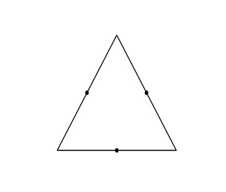
Figure 1: Three Edge Midpoints

We will now proceed to discuss the degrees 1 through 5 situations, based on sets of points introduced in [3]. The idea is to place a maximal number of points on the boundary of the simplex in $\mathbb{R}^{d}$, in such a way that restricted to a lower dimensional face of dimension $0\leq d^{\prime}<d$ we obtain the prescribed set of points for the simplex in $\mathbb{R}^{d^{\prime}}.$ On any edge, i.e. , a one dimensional face, we place the univariate Fekete points, which are known to be the zeros of $(x^{2}-1)P_{n}^{\prime}(x),$ where $P_{n}(x)$ is the $n$th classical Legendre polynomial.

1 Degree One

For degree one the dimension of the polynomials is $d+1.$

Proposition 1.1.

(cf. [3]) The set $F_{1}=X_{d}\subset S_{d}$ is a set of Fejèr points of degree one for all dimensions $d.$

Proof. The Lagrange polynomial for the $i$th vertex $V_{i}$ is just $\ell_{i}=\lambda_{i},$ in barycentric coordinates. Now, for $x\in S_{d},$ $\lambda_{i}\geq 0,$ $1\leq i\leq d+1$ and hence

$$\sum_{i=1}^{d+1}\ell_{i}^{2} =\sum_{i=1}^{d+1}\lambda_{i}^{2}$$

$$\leq\left(\sum_{i=1}^{d+1}\lambda_{i}\right)^{2}$$

$$=1.$$

$\square$

2 Degree Two

Let $F_{2}\subset S_{d}$ be the set consisting of the $d+1$ vertices together with the ${d+1\choose 2}$ edge midpoints. Note that

$$(d+1)+{d+1\choose 2}={d+2\choose 2}=N_{2}.$$

Proposition 2.1.

(cf. [3]) The set $F_{2}$ is a Fejèr set for all dimensions $d.$

Proof. It is easy to confirm that the Lagrange polynomial for vertex $V_{i}$ is $\lambda_{i}(2\lambda_{i}-1)$ while for the midpoint $(V_{i}+V_{j})/2$ it is $4\lambda_{i}\lambda_{j}.$

We make use of the symmetric power functions

$$p_{r}({\bm{\lambda}}):=\sum_{i=1}^{d+1}\lambda_{i}^{r}.$$

Note that for barycentric coordinates $p_{1}({\bm{\lambda}})=1,$ and hence

$$1-K_{2}({\bm{\lambda}}) =p_{1}^{4}-\sum_{i=1}^{d+1}\lambda_{i}^{2}(2\lambda_{i}-p_{1})^{2}-16\sum_{1\leq i<j\leq d+1}\lambda_{i}^{2}\lambda_{j}^{2}$$

$$=p_{1}^{4}-\sum_{i=1}^{d+1}\bigl{\{}4\lambda_{i}^{4}-4\lambda_{i}^{3}p_{1}+\lambda_{i}^{2}p_{1}^{2}\bigr{\}}-8(p_{2}^{2}-p_{4})$$

$$=p_{1}^{4}-\bigl{\{}4p_{4}-4p_{1}p_{3}+p_{1}^{2}p_{2}\bigr{\}}-8(p_{2}^{2}-p_{4})$$

$$=p_{1}^{4}+4p_{4}+4p_{1}p_{3}-p_{1}^{2}p_{2}-8p_{2}^{2}.$$

It can be shown, by brute force calculus, that this is always positive on the simplex $S_{d}.$

However, a perhaps more elegant solution is to notice, after some computation, that

$$1-K_{2}({\bm{\lambda}}) =6\sum_{j<k}\lambda_{j}\lambda_{k}(\lambda_{j}-\lambda_{k})^{2}+10\sum_{i<j<k}\lambda_{i}\lambda_{j}\lambda_{k}(\lambda_{i}+\lambda_{j}+\lambda_{k})$$

$$+24\sum_{i<j<k<m}\lambda_{i}\lambda_{j}\lambda_{k}\lambda_{m}$$

$$\geq 0,\quad{\bf x}\in S_{d}.$$

$\square$

Remark 2.2.

It is worthwhile noting that $1-K_{2}({\bf x})$ can also be analyzed using Schur functions. Indeed, for a partition ${\bm{\mu}}\in\mathbb{Z}_{+}^{m}$ with

$$\mu_{1}\geq\mu_{2}\geq\cdots\geq\mu_{m}\geq 0$$

one defines (cf. the monograph by Macdonald [12]), for ${\bf x}\in\mathbb{R}^{m},$

$$s_{\bm{\mu}}({\bf x})={\rm det}([x_{i}^{\mu_{j}+m-j}]_{1\leq i,j\leq m})/\prod_{1\leq i<j\leq m}(x_{i}-x_{j}).$$ (2.1)

The Schur functions are symmetric polynomials and indeed the Schur polynomials $s_{\bm{\mu}}(x_{1},\cdots,x_{m})$ with $|{\bm{\mu}}|=n,,$ form a $\mathbb{Z}$-basis for the homogeneous symmetric polynomials of degree $n$ with integer coefficients in $m$ variables.

In particular we may express $1-K_{2}({\bm{\lambda}})$ in terms of Schur polynomials, and indeed one may verify that in dimension $d$ with ${\bm{\lambda}}\in\mathbb{R}^{d+1},$

$$1-K_{2}=6s_{[3,1,0^{d-1}]}-18s_{[2,2,0^{d-1}]}+16s_{[2,1,1,0^{d-2}]}-6s_{[1,1,1,1,0^{d-3}]}.$$ (2.2)

Now it can also be verified that

$$\sum_{i<j}\lambda_{i}\lambda_{j}(\lambda_{i}-\lambda_{j})^{2}=s_{[3,1,0^{d-1}]}-3s_{[2,2,0^{d-1}]}+s_{[2,1,1,0^{d-2}]}$$

and so, in particular,

$$s_{[3,1,0^{d-1}]}-3s_{[2,2,0^{d-1}]}+s_{[2,1,1,0^{d-2}]}\geq 0.$$

Hence by (2.2),

$$1-K_{2} =6(s_{[3,1,0^{d-1}]}-3s_{[2,2,0^{d-1}]}+s_{[2,1,1,0^{d-2}]})+10s_{[2,1,1,0^{d-2}]}-6s_{[1,1,1,1,0^{d-3}]}$$

$$\geq 10s_{[2,1,1,0^{d-2}]}-6s_{[1,1,1,1,0^{d-3}]}.$$

We claim that the last expression is non-negative. To see this we use the inequality on normalized Schur functions given by Sra [13]. Specifically, write

$${\bm{\mu}}_{1}\succeq{\bm{\mu}}_{2}\,\,\iff\,\,\sum_{j=1}^{k}({\bm{\mu}_{1}})_{j}\geq\sum_{j=1}^{k}({\bm{\mu}}_{2})_{k},\,\,k=1,2\cdots.$$

Then, in case ${\bm{\mu}}_{1}\succeq{\bm{\mu}}_{2},$ for ${\bm{x}}\in\mathbb{R}_{+}^{m},$

$$\frac{s_{{\bm{\mu}}_{1}}({\bf x})}{s_{{\bm{\mu}}_{1}}(1^{m})}\geq\frac{s_{{\bm{\mu}}_{2}}({\bf x})}{s_{{\bm{\mu}}_{2}}(1^{m})}.$$ (2.3)

We may compute

$$s_{[2,1,1,0^{d-2}]}(1^{d+1})=3{d+2\choose 4},\,\,\,s_{[1,1,1,1,0^{d-3}]}(1^{d+1})={d+1\choose 4}.$$

Consequently,

$$s_{[2,1,1,0^{d-2}]}\geq 3\frac{d+2}{d-2}\times s_{[1,1,1,1,0^{d-3}]}$$

from which our claim follows easily. $\square$

3 Degree Three

Let $F_{3}\subset S_{d}$ be the set consisting of the $d+1$ vertices together with the $2{d+1\choose 2}$ edge points $tV_{i}+(1-t)V_{j},$ $i\neq j,$ $t=(1+1/\sqrt{5})/2,$ together with the ${d+1\choose 3}$ barycentres of each two-dimensional face.

Note that

$$(d+1)+2{d+1\choose 2}+{d+1\choose 3}={d+3\choose 3}=N_{3}.$$

We conjecture that $F_{3}$ is a Fejèr set for all dimensions, but can only prove this for dimensions up to 28.

Proposition 3.1.

(cf. [3]) $F_{3}$ is a Fejèr set for dimensions $1\leq d\leq 28.$

Proof. The $d=1$ case is a special case of Fejèr’s original theorem [7]. Otherwise, we note (as given in [3]) that for the vertex $V_{i},$

$$\ell_{i}=(\lambda_{i}/2)(12\lambda_{i}^{2}-12\lambda_{i}+3-S_{2})$$

where $S_{k}:=\sum_{i=1}^{d+1}\lambda_{i}^{k};$ while for the face midpoint $(V_{i}+V_{j}+V_{k})/3,$ $i<j<k,$

$$\ell_{ijk}=27\lambda_{i}\lambda_{j}\lambda_{k},$$

and for the edge points $tV_{i}+(1-t)V_{j},$ $i\neq j,$

$$\ell_{ij}=5\lambda_{i}\lambda_{j}((1+t\sqrt{5})\lambda_{i}+(2-t\sqrt{5})\lambda_{j}-1).$$

The $d=2$ case is special, as there is a single point, in the interior of $S_{2}$ (at the barycentre). We let, for simplicity’s sake, $x,y,z$ denote the three barycentric coordinates and compute

$$K(x,y,z) :=\sum_{i=1}^{10}\ell_{i}^{2}(x,y,z)$$

$$={z}^{6}-6\,y\,{z}^{5}-6\,x\,{z}^{5}+87\,{y}^{2}\,{z}^{4}+24\,x\,y\,{z}^{4}+87\,{x}^{2}\,{z}^{4}-112\,{y}^{3}\,{z}^{3}$$

$$-68\,x\,{y}^{2}\,{z}^{3}-68\,{x}^{2}\,y\,{z}^{3}-112\,{x}^{3}\,{z}^{3}+87\,{y}^{4}\,{z}^{2}-68\,x\,{y}^{3}\,{z}^{2}$$

$$+912\,{x}^{2}\,{y}^{2}\,{z}^{2}-68\,{x}^{3}\,y\,{z}^{2}+87\,{x}^{4}\,{z}^{2}-6\,{y}^{5}\,z+24\,x\,{y}^{4}\,z-68\,{x}^{2}\,{y}^{3}\,z$$

$$-68\,{x}^{3}\,{y}^{2}\,z+24\,{x}^{4}\,y\,z-6\,{x}^{5}\,z+{y}^{6}-6\,x\,{y}^{5}+87\,{x}^{2}\,{y}^{4}-112\,{x}^{3}\,{y}^{3}$$

$$+87\,{x}^{4}\,{y}^{2}-6\,{x}^{5}\,y+{x}^{6}$$

so that

$$H(x,y,z) :=1-K(x,y,z)$$

$$=(x+y+z)^{6}-K(x,y,z)$$

$$=12\,y\,{z}^{5}+12\,x\,{z}^{5}-72\,{y}^{2}\,{z}^{4}+6\,x\,y\,{z}^{4}-72\,{x}^{2}\,{z}^{4}+132\,{y}^{3}\,{z}^{3}$$

$$+128\,x\,{y}^{2}\,{z}^{3}+128\,{x}^{2}\,y\,{z}^{3}+132\,{x}^{3}\,{z}^{3}-72\,{y}^{4}\,{z}^{2}+128\,x\,{y}^{3}\,{z}^{2}$$

$$-822\,{x}^{2}\,{y}^{2}\,{z}^{2}+128\,{x}^{3}\,y\,{z}^{2}-72\,{x}^{4}\,{z}^{2}+12\,{y}^{5}\,z+6\,x\,{y}^{4}\,z$$

$$+128\,{x}^{2}\,{y}^{3}\,z+128\,{x}^{3}\,{y}^{2}\,z+6\,{x}^{4}\,y\,z+12\,{x}^{5}\,z+12\,x\,{y}^{5}$$

$$-72\,{x}^{2}\,{y}^{4}+132\,{x}^{3}\,{y}^{3}-72\,{x}^{4}\,{y}^{2}+12\,{x}^{5}\,y.$$

We are claiming that $H(x,y,z)\geq 0$ for $x,y,z\geq 0,$ $x+y+z=1.$ Certainly this would be the case if all the coefficients were non-negative. However, $H(x,y,z)=0$ at the barycentre and hence it is not possible to have all non-negative coefficients. To overcome this problem we re-express $H$ in terms of the barycentric coordinates for the subtriangle with vertices $V_{1},$ $V_{2}$ and the barycentre $(V_{1}+V_{2}+V_{3})/3.$ If $H\geq 0$ on this subtriangle then, by symmetry, it will be non-negative on the whole simplex.

Let therefore $(u,v,w)$ be the barycentric coordinates with repsect to this subtriangle. Then

$$x=u+w/3,\,\,y=v+w/3,\,\,z=w/3$$

and $H$ becomes

$$H(u,v,w) =\frac{2}{81}\{131\,{v}^{2}\,{w}^{4}-131\,u\,v\,{w}^{4}+131\,{u}^{2}\,{w}^{4}+312\,{v}^{3}\,{w}^{3}+318\,u\,{v}^{2}\,{w}^{3}$$

$$+318\,{u}^{2}\,v\,{w}^{3}+312\,{u}^{3}\,{w}^{3}-81\,{v}^{4}\,{w}^{2}+1566\,u\,{v}^{3}\,{w}^{2}+1215\,{u}^{2}\,{v}^{2}\,{w}^{2}$$

$$+1566\,{u}^{3}\,v\,{w}^{2}-81\,{u}^{4}\,{w}^{2}+324\,{v}^{5}\,w-1053\,u\,{v}^{4}\,w+3186\,{u}^{2}\,{v}^{3}\,w$$

$$+3186\,{u}^{3}\,{v}^{2}\,w-1053\,{u}^{4}\,v\,w+324\,{u}^{5}\,w+486\,u\,{v}^{5}-2916\,{u}^{2}\,{v}^{4}$$

$$+5346\,{u}^{3}\,{v}^{3}-2916\,{u}^{4}\,{v}^{2}+486\,{u}^{5}\,v\}.$$

Then

$$H= \frac{262\,\left({v}^{2}-u\,v+{u}^{2}\right)\,{w}^{4}}{81}+12\,u\,v\,\left({v}^{2}-3\,u\,v+{u}^{2}\right)^{2}+\frac{2w}{27}\{104\,{v}^{3}\,{w}^{2}$$

$$+106\,u\,{v}^{2}\,{w}^{2}+106\,{u}^{2}\,v\,{w}^{2}+104\,{u}^{3}\,{w}^{2}-27\,{v}^{4}\,w+522\,u\,{v}^{3}\,w$$

$$+405\,{u}^{2}\,{v}^{2}\,w+522\,{u}^{3}\,v\,w-27\,{u}^{4}\,w+108\,{v}^{5}$$

$$-351\,u\,{v}^{4}+1062\,{u}^{2}\,{v}^{3}+1062\,{u}^{3}\,{v}^{2}-351\,{u}^{4}\,v+108\,{u}^{5}\}.$$

To show that $H\geq 0$ for $u,v,w\geq 0,$ $u+v+w=1,$ we note that as the first two terms above are both positive, it suffices to show that the expression in the brace brackets is also positive. Let $E$ denote this expression.

However,

$$(u+v+w)^{4}E =104\,{v}^{3}\,{w}^{6}+106\,u\,{v}^{2}\,{w}^{6}+106\,{u}^{2}\,v\,{w}^{6}+104\,{u}^{3}\,{w}^{6}$$

$$+389\,{v}^{4}\,{w}^{5}+1362\,u\,{v}^{3}\,{w}^{5}+1253\,{u}^{2}\,{v}^{2}\,{w}^{5}+1362\,{u}^{3}\,v\,{w}^{5}$$

$$+389\,{u}^{4}\,{w}^{5}+624\,{v}^{5}\,{w}^{4}+3513\,u\,{v}^{4}\,{w}^{4}$$

$$+7302\,{u}^{2}\,{v}^{3}\,{w}^{4}+7302\,{u}^{3}\,{v}^{2}\,{w}^{4}+3513\,{u}^{4}\,v\,{w}^{4}+624\,{u}^{5}\,{w}^{4}$$

$$+686\,{v}^{6}\,{w}^{3}+3508\,u\,{v}^{5}\,{w}^{3}+14320\,{u}^{2}\,{v}^{4}\,{w}^{3}+22996\,{u}^{3}\,{v}^{3}\,{w}^{3}$$

$$+14320\,{u}^{4}\,{v}^{2}\,{w}^{3}+3508\,{u}^{5}\,v\,{w}^{3}+686\,{u}^{6}\,{w}^{3}+644\,{v}^{7}\,{w}^{2}$$

$$+1476\,u\,{v}^{6}\,{w}^{2}+11522\,{u}^{2}\,{v}^{5}\,{w}^{2}+31694\,{u}^{3}\,{v}^{4}\,{w}^{2}$$

$$+31694\,{u}^{4}\,{v}^{3}\,{w}^{2}+11522\,{u}^{5}\,{v}^{2}\,{w}^{2}+1476\,{u}^{6}\,v\,{w}^{2}+644\,{u}^{7}\,{w}^{2}$$

$$+405\,{v}^{8}\,w+306\,u\,{v}^{7}\,w+3663\,{u}^{2}\,{v}^{6}\,w+18378\,{u}^{3}\,{v}^{5}\,w$$

$$+29232\,{u}^{4}\,{v}^{4}\,w+18378\,{u}^{5}\,{v}^{3}\,w+3663\,{u}^{6}\,{v}^{2}\,w+306\,{u}^{7}\,v\,w$$

$$+405\,{u}^{8}\,w+108\,{v}^{9}+81\,u\,{v}^{8}+306\,{u}^{2}\,{v}^{7}+3636\,{u}^{3}\,{v}^{6}+8973\,{u}^{4}\,{v}^{5}$$

$$+8973\,{u}^{5}\,{v}^{4}+3636\,{u}^{6}\,{v}^{3}+306\,{u}^{7}\,{v}^{2}+81\,{u}^{8}\,v+108\,{u}^{9}$$

which is positive as each term has a positive coefficient.

For $d\geq 3$ there are no longer interior points and there is a simple algebraic procedure to verify that $1-K_{3}\geq 0$ on the simplex. We proceed by induction. Assuming that $F_{3}$ is a Fejèr set for dimension $d-1$ one calculates $1-K_{3}$ in homogenized form

$$\Bigl{(}\sum_{j=1}^{d+1}\lambda_{j}\Bigr{)}^{6}-K_{3}({\bm{\lambda}})$$

and then considers this on the sub-simplex with vertices

$$V_{1},\cdots,V_{d},(V_{1}+\cdots+V_{d+1})/(d+1).$$

If we let $\mu_{1},\cdots,\mu_{d+1}$ be the barycentric coordinates for the sub-simplex, then it is easy to see that

$$\lambda_{j}=\mu_{j}+\mu_{d+1}/(d+1),\,\,1\leq j\leq d,\quad\lambda_{d+1}=\mu_{d+1}/(d+1).$$ (3.1)

Let $H({\bm{\mu}})$ be $1-K_{3}$ restricted to this sub-simplex, i.e.,

$$H({\bm{\mu}})=\Bigl{(}\sum_{j=1}^{d+1}\lambda_{j}\Bigr{)}^{6}-K_{3}({\bm{\lambda}})$$

with ${\bm{\lambda}}$ given by (3.1). It is sufficient to prove that $H({\bm{\mu}})\geq 0$ for $\mu_{j}\geq 0,$ $1\leq j\leq(d+1)$ for which it is, in turn, sufficient to show that

$$H({\bm{\mu}})-H(\widehat{{\bm{\mu}}},0)\geq 0,\quad\widehat{{\bm{\mu}}}:=(\mu_{1},\mu_{2},\cdots,\mu_{d})$$

as the term $H(\widehat{{\bm{\mu}}},0)$ is the restriction of $H$ to the face $\mu_{d+1}=\lambda_{d+1}=0$ and hence is positive by the induction hypothesis.

For positivity it is sufficient that, for some integer $r\geq 0,$ all the coefficients of

$$\Bigl{(}\sum_{j=1}^{d+1}\mu_{j}\Bigr{)}^{r}(H({\bm{\mu}})-H(\widehat{{\bm{\mu}}},0))$$

are non-negative. This has been verified by means of computer algebra for degrees up to 28 with $r=8$ for dimension $d=3,$ $r=5$ for $d=4,$ $r=3$ for $d=5,6$ and $r=2$ otherwise. Appendix A gives Matlab code using its Symbolic Toolbox for this purpose. $\square$

Remark 3.2.

Multiplying a polynomial in barycentric coordinates by one in the form of $\sum_{j=1}^{d+1}\mu_{j}$ is known as degree elevation. The minimal $r$ necessary to have all non-negative coefficients is connected to the so-called Bernstein degree of a polynomial which is positive on a simplex. $\square$

4 Degree Four

Let $F_{4}\subset S_{d}$ be the set of points introduced in [3] consisting of

• the ${d+1\choose 4}$ centres of each three dimesnional face:

  $$\frac{1}{4}(V_{i}+V_{j}+V_{k}+V_{\ell}),\,\,i<j<k<\ell$$

• the $3{d+1\choose 3}$ vertices of a triangle in the interior of each two dimensional face:

  $$\frac{4+\sqrt{5}}{11}V_{i}+\frac{7-\sqrt{5}}{22}(V_{j}+V_{k}),\,\,i\neq j,k,\,\,j<k$$

• the $3{d+1\choose 2}$ points with 3 points on each edge (1 dimensional face):

  $$\frac{1-\sqrt{3/7}}{2}V_{i}+\frac{1+\sqrt{3/7}}{2}V_{j},\,\,i\neq j,$$

  $$\frac{1}{2}(V_{i}+V_{j}),\,\,i<j$$

• the $d+1$ vertices $V_{i}.$

We note that the cardinality of $F_{4}$ is

$${d+1\choose 4}+3{d+1\choose 3}+3{d+1\choose 2}+(d+1)={d+4\choose 4}=N_{4}.$$

The associated Lagrange polynomials are also given in [3], which, for the sake of completeness, we reproduce here:

• $\ell_{ijk\ell}=256\lambda_{i}\lambda_{j}\lambda_{k}\lambda_{\ell}$

• $\displaystyle{\ell_{ijk}=\frac{73+\sqrt{5}}{2}\lambda_{i}\lambda_{j}\lambda_{k}\Bigl{\{}(1+\sqrt{5})\lambda_{i}+\frac{3-\sqrt{5}}{2}(\lambda_{j}+\lambda_{k})-1\Bigr{\}}}$

• $$\ell_{ij} =\frac{49}{6}\lambda_{i}\lambda_{j}\Bigl{\{}\bigl{(}\frac{61+7\sqrt{5}}{22}-\sqrt{3/7}\frac{7+\sqrt{5}}{2}\bigr{)}\lambda_{i}^{2}$$

  $$+\frac{3+9\sqrt{5}}{11}\lambda_{i}\lambda_{j}+\bigl{(}\frac{61+7\sqrt{5}}{22}+\sqrt{3/7}\frac{7+\sqrt{5}}{2}\bigr{)}\lambda_{j}^{2}$$

  $$+\bigl{(}\sqrt{3/7}\frac{5+\sqrt{5}}{2}-\frac{41+13\sqrt{5}}{22}\bigr{)}\lambda_{i}$$

  $$-\bigl{(}\sqrt{3/7}\frac{5+\sqrt{5}}{2}+\frac{41+13\sqrt{5}}{22}\bigr{)}\lambda_{i}$$

  $$+\frac{8+2\sqrt{5}}{11}-\frac{7-\sqrt{5}}{11}S_{2}\Bigl{\}}$$

• $$\ell_{ij} =\frac{4}{33}\lambda_{i}\lambda_{j}\Bigl{\{}(100-8\sqrt{5})(\lambda_{i}^{2}+\lambda_{j}^{2})+(672-96\sqrt{5})\lambda_{i}\lambda_{j}$$

  $$+(62\sqrt{5}-302)(\lambda_{i}+\lambda_{j})+(82-40\sqrt{5})S_{2}\Bigr{\}}$$

• $$\ell_{i} =2\lambda_{i}\Bigl{\{}\frac{101+17\sqrt{5}}{11}\lambda_{i}^{3}-(13+2\sqrt{5})\lambda_{i}^{2}+\frac{130+27\sqrt{5}}{22}\lambda_{i}$$

  $$-\frac{259+51\sqrt{5}}{264}+S_{2}\bigl{(}\frac{9+\sqrt{5}}{8}-\frac{24+17\sqrt{5}}{22}\lambda_{i}\bigr{)}$$

  $$+S_{3}\bigl{(}\frac{45+3\sqrt{5}}{44}-\frac{5}{3}\bigr{)}\Bigr{\}}.$$

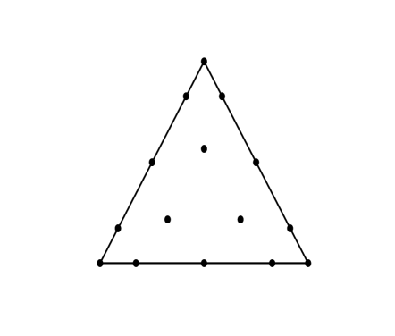
Figure 2: The 15 Points for Degree 4

It is shown in [3] that for $d=2,$ $F_{4}$ is a Fejèr set.

Proposition 4.1.

In dimension $d=2$ we have, for the set $F_{4},$

$$\sum_{i=1}^{N}\ell_{i}^{2}({\bf x})\leq 1,\,\,{\bf x}\in S_{2}.$$

Extensive numerical calculations indicate that this is also the case in dimension $d=3.$

Conjecture 4.2.

In dimension $d=3$ we have, for the set $F_{4},$

$$\sum_{i=1}^{N}\ell_{i}^{2}({\bf x})\leq 1,\,\,{\bf x}\in S_{3}.$$

However, it is not the case in dimension $d=4.$ Indeed, by direct calculation we see that for ${\bf x}=(V_{1}+V_{2}+V_{3}+V_{4}+V_{5})/5,$ the centroid of $S_{4},$

$$\sum_{i=1}^{N}\ell_{i}^{2}({\bf x})=\frac{80243\sqrt{5}+9298842}{9453125}=1.00266...>1.$$

We nevertheless conjecture

Conjecture 4.3.

The sets $F_{4}$ are Fekete sets for all dimensions $d=1,2,\cdots.$

As evidence for this conjecture we can prove that for dimensions $d=3,4,5,6,7$ the Lagrange polynomials for $F_{4}$ satisfy the necessary (but not sufficient) condition that they are all bounded by 1. Indeed, somewhat more is true.

Proposition 4.4.

The Lagrange polynomials for the centroids of each 3-face,

$$\ell_{ijk\ell}=256\lambda_{i}\lambda_{j}\lambda_{k}\lambda_{\ell}=256\lambda_{i}\lambda_{j}\lambda_{k}\lambda_{\ell}$$

are bounded by 1 in absolute value on $S_{d}$ for any dimension ($d\geq 3$). Further, the sum of all the other Lagrange polynomials squared is bounded by 1 on $S_{d}$ for $d=3,4,5,6,7.$

Proof. The first statement amounts to showing that $256xyzw\leq 1$ for $x,y,z,w\geq 0$ and $x+y+z+w\leq 1,$ but this is an elementary verification.

For the second statement, we calculate, just as in the proof of Prop. 3.1, the sum of the stated Lagrange polynomials squared and again reduce to the sub-simplex with vertices $V_{1},\cdots,V_{d}$ and the centroid $\displaystyle{\frac{1}{d+1}\sum_{j=1}^{d+1}V_{j}.}$ Letting $\mu_{j},$ $1\leq j\leq(d+1)$ denote the barycentric coordinates of this sub-simplex, we then have

$$\lambda_{j} =\mu_{j}+\frac{1}{d+1}\mu_{d+1},\,\,1\leq j\leq d,$$ (4.1)

$$\lambda_{d+1} =\frac{1}{d+1}\mu_{d+1}.$$ (4.2)

Let $H({\bm{\mu}})$ be $1-K_{4}$ restricted to this sub-simplex, i.e.,

$$H({\bm{\mu}})=\Bigl{(}\sum_{j=1}^{d+1}\lambda_{j}\Bigr{)}^{8}-K_{4}({\bm{\lambda}})$$

with ${\bm{\lambda}}$ given by (4.1). It is sufficient to prove that $H({\bm{\mu}})\geq 0$ for $\mu_{j}\geq 0,$ $1\leq j\leq(d+1)$ for which it is, in turn, sufficient to show that

$$H({\bm{\mu}})-H(\widehat{{\bm{\mu}}},0)\geq 0,\quad\widehat{{\bm{\mu}}}:=(\mu_{1},\mu_{2},\cdots,\mu_{d})$$

as the term $H(\widehat{{\bm{\mu}}},0)$ is the restriction of $H$ to the face $\mu_{d+1}=\lambda_{d+1}=0$ which we may assume to be positive by induction.

For positivity it is again sufficient that, for some integer $r\geq 0,$ all the coefficients of

$$\Bigl{(}\sum_{j=1}^{d+1}\mu_{j}\Bigr{)}^{r}(H({\bm{\mu}})-H(\widehat{{\bm{\mu}}},0))$$

are non-negative. This has been verified by means of computer algebra for degrees up to 7 with $r=11$ for dimension $d=3,$ $r=8$ for $d=4,$ $r=7$ for $d=5,6$ and $r=8$ for $d=7.$ $\square$

Remark 4.5.

One could of course continue this procedure dimension by dimension, but a general proof is much to be preferred. $\square$

Numerical computations indicate that, at least for dimensions $d=3,4,5,$ the sum of the fourth powers of the Lagrange polynomials is bounded by 1.

Conjecture 4.6.

For all dimensions $d\geq 1,$ we have

$$\sum_{j=1}^{N}\ell_{j}^{4}({\bf x})\leq 1,\,\,{\bf x}\in S_{d}$$

or, in other words,

$$\|{\bm{\ell}}({\bf x})\|_{4}\leq 1,\,\,{\bf x}\in S_{d}.$$

Remark 4.7.

We use the fourth power in order to remain in the domain of polynomials. However, numerical computations indicate that there is a smaller exponent

$$r\approx 2.00217448$$

such that

$$\|{\bm{\ell}}({\bf x})\|_{r}\leq 1,\,\,{\bf x}\in S_{d},\,\,d=4,5.$$

This leads us to formulate the following definition

Definition 4.8.

Suppose that $X\subset S_{d}$ is a subset of $N_{n}$ points for which $\|{\bm{\ell}}({\bf x})\|_{\infty}\leq 1,$ ${\bf x}\in S_{d}.$ We define the Fejér exponent of $X$ to be that $r\in[2,\infty]$ for which

$$\|{\bm{\ell}}({\bf x})\|_{r}\leq 1,\,\,{\bf x}\in S_{d}$$

and for which for $r^{\prime}<r,$

$$\max_{{\bf x}\in S_{d}}\|{\bm{\ell}}({\bf x})\|_{r^{\prime}}>1.$$

$\square$

We speculate that the Fekete points have minimal Fejér exponent.

5 Degree Five

For degree 5 we are able to give explicit formulas for the points on the edges but can express the points in the interior of the 2-faces only in terms of the roots of a certain polynomial. Consequently this section will be largely numerical.

We describe first the set of points $F_{5}$ in $\mathbb{R}^{2}.$ The dimension of the space of polynomials of degree at most five in two variables is $N_{2}={5+2\choose 2}=21.$ $F_{5}$ will consist of the 3 vertices together with 4 additional points on each of the 3 edges, leaving 21-15=6 points to be placed in the interior of the triangle. The 4 interior edge points are just the interior univariate Fekete points of degree 5, i.e., the zeros of $P_{5}^{\prime}(x),$ the derivative of the Legendre polynomial of degree 5. Now

$$P_{5}(x)=\frac{1}{8}\bigl{(}63x^{5}-70x^{3}+15x\bigr{)}$$

and hence

$$P_{5}^{\prime}(x)=\frac{15}{8}\bigl{(}21x^{4}-14x^{2}+1\bigr{)}$$

with zeros

$$z=\pm\sqrt{\frac{7\pm 2\sqrt{7}}{21}}$$

with barycentric coordinates

$$\Bigr{(}\frac{1-z}{2},\frac{1+z}{2}\Bigr{)}.$$

For the 6 interior points, we assume that these are symmetric and have barycentric coordinates

$$(u,u,1-2u),\,\,(u,1-2u,u),\,\,(1-2u,u,u)$$

$$(v,v,1-2v),\,\,(v,1-2v,v),\,\,(1-2v,v,v)$$

for some parameters $u,v\in(0,1).$ Now, the polynomials of degree 5 of the form $\lambda_{1}\lambda_{2}\lambda_{3}q({\bm{\lambda}}),$ for some quadrtic $q,$ are all zero at the boundary points. Hence the Vandermonde determinant of all 21 points will decouple into a factor depending on the boundary points (given) and the Vandermonde determinant for the 6 interior points with basis $\lambda_{1}\lambda_{2}\lambda_{3}q({\bm{\lambda}})$ for

$$q\in\{\lambda_{1}^{2},\lambda_{2}^{2},\lambda_{3}^{2},\lambda_{1}\lambda_{2},\lambda_{1}\lambda_{3},\lambda_{2}\lambda_{3}\}.$$

(See e.g. [5] for a discussion of this kind of factorization for Vandermonde determinants). We obtain therefore that there is some constant $C$ such that

$${\rm vdm}=C(u^{2}(1-2u))^{3}(v^{2}(1-2v))^{3}\times$$

$$\left|\begin{array}[]{cccccc}u^{2}&u^{2}&(1-2u)^{2}&u^{2}&u(1-2u)&u(1-2u)\cr u^{2}&(1-2u)^{2}&u^{2}&u(1-2u)&u^{2}&u(1-2u)\cr(1-2u)^{2}&u^{2}&u^{2}&u(1-2u)&u(1-2u)&u^{2}\cr v^{2}&v^{2}&(1-2v)^{2}&v^{2}&v(1-2v)&v(1-2v)\cr v^{2}&(1-2v)^{2}&v^{2}&v(1-2v)&v^{2}&v(1-2v)\cr(1-2v)^{2}&v^{2}&v^{2}&v(1-2v)&v(1-2v)&v^{2}\end{array}\right|$$

$$=C(u^{2}(1-2u))^{3}(v^{2}(1-2v))^{3}\times$$

$$(u-v)^{3}(3u-1)^{2}(3v-1)^{2}(3(u+v)-2)$$

after a short calculation.

Hence we wish to maximize

$$p(u,v):=(u-v)^{3}u^{6}v^{6}(2u-1)^{3}(2v-1)^{3}(3u-1)^{2}(3v-1)^{2}(3(u+v)-2).$$

The partial derivatives are

$$\frac{\partial p}{\partial u} =6(u-v)^{2}u^{5}v^{6}(2v-1)^{3}(3v-1)^{2}(2u-1)^{2}(3u-1)\times$$

$$\,\,\,\bigl{(}45u^{4}+6u^{3}v-59u^{3}-33u^{2}v^{2}+17u^{2}v+24u^{2}+21uv^{2}-13uv-3u-3v^{2}+2v\bigr{)}$$

$$\frac{\partial p}{\partial v} =6(u-v)^{2}u^{6}v^{5}(2u-1)^{3}(2v-1)^{2}(3u-1)^{2}(3v-1)\times$$

$$\,\,\,\bigl{(}33u^{2}v^{2}-21u^{2}v+3u^{2}-6uv^{3}-17uv^{2}+13uv-2u-45v^{4}+59v^{3}-24v^{2}+3v\bigr{)}.$$

We seek to find the critical points given by the common zeros of the factors

$$q_{1}(u,v) =45u^{4}+6u^{3}v-59u^{3}-33u^{2}v^{2}+17u^{2}v+24u^{2}+21uv^{2}-13uv-3u-3v^{2}+2v,$$

$$q_{2}(u,v) =33u^{2}v^{2}-21u^{2}v+3u^{2}-6uv^{3}-17uv^{2}+13uv-2u-45v^{4}+59v^{3}-24v^{2}+3v.$$

Upon calculating a Groebner basis of these polynomials one finds that these common zeros are determined by the univariate polynomial

$$q(v) =2737800v^{10}-8660340v^{9}+11981963v^{8}-9523289v^{7}$$

$$\,\,\,+4800577v^{6}-1598001v^{5}+354286v^{4}-51415v^{3}+4649v^{2}-235v+5$$

whose roots may be calculated to any precision desired. By trial and error we find that the roots near

$$u =0.148019471315134,$$

$$v =0.420825539292557$$

give the largest determinant, and we use these.

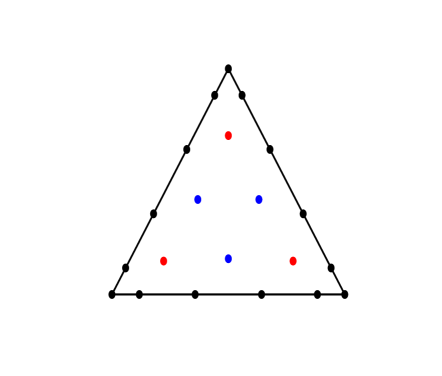
Figure 3: The 21 Points for Degree 5

Remark 5.1.

Although the 6 interior points appear visually to all be on an interior triangle, close inspection of the coordinates reveals that this is not the case. $\square$

Numerical Example 5.2.

For dimension $d=2,$ the set $F_{5}$ of the 21 points defined above do not form a Fejér set. Indeed,

$$\max_{{\bf x}\in S_{2}}\sum_{i=1}^{21}\ell_{i}^{2}({\bf x})\approx 1.2246$$

which is attained at the centroid $(1/3,1/3,1/3).$

However, we do believe that they are Fekete points. Indeed it’s Fejér exponent is

$$r\approx 2.2513.$$

In particular, all the Lagrange polynomials are bounded by 1 in absolute value on $S_{2}.$ $\square$

We now proceed to dimension $d=3.$ Here the dimension of the space of polynomials of degree at most 5 is

$$N_{5}={5+3\choose 3}=56.$$

The set $F_{5}$ is such that restricted to any 2-face we obtain its two-dimensional version, i.e., we place 1 point at each of the 4 vertices, 4 interior points on each of the 6 edges and 6 interior points on each of the 4 2-faces, for a total of $4+4\times 6+6\times 4=52$ boundary points. This leaves $56-52=4$ points to be placed in the interior of the simplex. By symmetry we assume that these are

$$(1-3w,w,w,w)$$ (5.1)

$$(w,1-3w,w,w),$$ (5.2)

$$(w,w,1-3w,w),$$ (5.3)

$$(w,w,w,1-3w)$$ (5.4)

for some parameter $w\in(0,1/3).$

The polynomials of the form

$$\lambda_{1}\lambda_{2}\lambda_{3}\lambda_{4}q({\bm{\lambda}}),\,\,{\rm deg}(q)\leq 1$$

are all zero on the boundary. Hence (cf. [5]) the Vandermonde determinant for the 56 points will factor into a constant (depending on the boundary points) times the Vandermonde determinant for the 4 points (5.1) with basis

$$\lambda_{1}\lambda_{2}\lambda_{3}\lambda_{4}\{\lambda_{1},\lambda_{2},\lambda_{3},\lambda_{4}\}$$

i.e.,

$$(w^{3}(1-3w))^{4}\,\,\left|\begin{array}[]{cccc}1-3w&w&w&w\cr w&1-3w&w&w\cr w&w&1-3w&w\cr w&w&w&1-3w\end{array}\right|$$

$$=(w^{3}(1-3w))^{4}(1-4w)^{3}.$$

The derivative of this expression with respect to $w$ is

$$12w^{11}(1-3w)^{3}(1-4w)^{2}(19w^{2}-9w+1)$$

with non-extraneous crtical points

$$w=\frac{9\pm\sqrt{5}}{38}.$$

Now, it turns out that the critical point $(9+\sqrt{5})/38$ is a local maximum for the absolute value of the determinant and $(9-\sqrt{5})/38$ the global maximum. Hence we take

$$w=\frac{9-\sqrt{5}}{38}.$$ (5.5)

Numerical Example 5.3.

There is a curious behaviour here. For both choises of $w=(9\pm\sqrt{5})/38,$ the Lagrange polynomials are all bounded by one in absoliute value, i.e.,

$$\|{\bm{\ell}}({\bf x})\|_{\infty}\leq 1,\,\,{\bf x}\in S_{3}.$$

However, the choice of $w=(9-\sqrt{5})/38$ produces a strictly larger Vandermonde determinant and hence only with this choice of $w$ can $F_{5}$ be a Fekete set, which we conjecture to be the case.

It is also interesting to note that with $w=(9+\sqrt{5})/38,$ the Fejér exponent is $>4,$ wheras for $w=(9-\sqrt{5})/38,$ the Fejér exponent remains, as in dimension $d=2,$

$$r\approx 2.2513.$$

$\square$

Moving to dimension $d=4,$

$$N_{5}={5+4\choose 4}=126.$$

We again place points on the boundary so that restricted to any 3-face we have $F_{5}$ for dimension 3. In this way we have 5 vertex points, 4 interior points on each of the ${5\choose 2}=10$ edges, 6 interior points on each of the ${5\choose 3}=10$ 2-faces and 4 interior points on each of the ${5\choose 4}=5$ 3-faces, for a total of $5+4\times 10+6\times 10+4\times 5=125$ boundary points so that there is but $1=126-125$ to be placed in the interior of the simplex. We put this point at the centroid $(1/5,1/5,1/5,1/5,1/5).$

Numerical Example 5.4.

We conjecture that the set $F_{5}$ of 126 points so constructed is a Fekete set. Indeed it remains the case that the Fejér exponent is

$$r\approx 2.2513$$

and so, in particular, all the Lagrange polynomials are bounded by 1 in absolute value. $\square$

In general we let $F_{5}$ be the set of points consisting of

• the ${d+1\choose 5}$ centres of each four dimesnional face:

  $$\frac{1}{5}(V_{i}+V_{j}+V_{k}+V_{\ell}+V_{m}),\,\,i<j<k<\ell<m$$

• the $4{d+1\choose 4}$ vertices of the simplex in the interior of each three dimensional face:

  $$(1-3w)V_{i}+wV_{j}+wV_{k}+wV_{\ell},$$

  $$wV_{i}+(1-3w)V_{j}+wV_{k}+wV_{\ell},$$

  $$wV_{i}+wV_{j}+(1-3w)V_{k}+wV_{\ell},$$

  $$wV_{i}+wV_{j}+wV_{k}+(1-3w)V_{\ell}$$

  for $i<j<k<\ell$ and $w=(9-\sqrt{5})/38.$

• the $6{d+1\choose 3}$ points in each 2-face:

  $$(1-2u)V_{i}+uV_{j}+uV_{k},$$

  $$uV_{i}+(1-2u)V_{j}+uV_{k},$$

  $$uV_{i}+uV_{j}+(1-2u)V_{k},$$

  $$(1-2v)V_{i}+vV_{j}+vV_{k},$$

  $$vV_{i}+(1-2v)V_{j}+vV_{k},$$

  $$vV_{i}+vV_{j}+(1-2v)V_{k}$$

  for $i<j<k$ and $u,v$ two of the roots of

  $$q(v) =2737800v^{10}-8660340v^{9}+11981963v^{8}-9523289v^{7}$$

  $$\,\,\,+4800577v^{6}-1598001v^{5}+354286v^{4}-51415v^{3}+4649v^{2}-235v+5$$

  near $u=0.148019471315134,$ $v=0.420825539292557.$

• the $4{d+1\choose 2}$ interior edge points:

  $$\lambda V_{i}+(1-\lambda)V_{j}$$

  for $i<j$ and $\lambda=(1-z)/2,$ $\displaystyle{z=\pm\sqrt{\frac{7\pm 2\sqrt{7}}{21}}}$

• the $(d+1)$ vertices $V_{i}.$

We note that the cardinality of $F_{5}$ is

$$\#(F_{5}) ={d+1\choose 5}+4{d+1\choose 4}+6{d+1\choose 3}+4{d+1\choose 2}+{d+1\choose 1}$$

$$={d+1\choose 5}$$

$$=N_{5}.$$

Appendix A

⬇

1%

2% test the positivity of 1-K_3 on the d-dimensional sub-simplex

3% with vertices V_1,…V_d and the barycentre (V_1+…V_{d+1})/(d+1)

4% of the simplex with vertices V_1,…V_{d+1} in R^d

5%

6clear all

7syms K t s1 s2

8d=input(’Desired dimension: ’)

9x=sym(’x’,[d+1 1]); % barycentric coordinates for the whole simplex

10y=sym(’y’,[d+1 1]); % barycentric coordinates for the sub-simplex

11%

12% find K, the sum of the squares of the Lagrange polynomials on the simplex

13%

14t=(1+1/sym(sqrt(5)))/2;

15s1=sum(x);

16s2=sum(x.^2);

17K=0;

18for i=1:(d+1)

19 K=K+(x(i)/2*(12*x(i)^2-12*x(i)*s1+3*s1^2-s2))^2;

20end

21for i=1:(d+1)

22 for j=1:(i-1)

23 K=K+(5*x(i)*x(j)*((1+sym(sqrt(5))*t)*x(i)+(2-sym(sqrt(5))*t) …

24 *x(j)-s1))^2;

25 K=K+(5*x(i)*x(j)*((1+sym(sqrt(5))*t)*x(j)+(2-sym(sqrt(5))*t) …

26 *x(i)-s1))^2;

27 end

28end

29for i=1:(d+1)

30 for j=1:(i-1)

31 for k=1:(j-1)

32 K=K+(27*x(i)*x(j)*x(k))^2;

33 end

34 end

35end

36K=expand(K);

37f=expand(s1^6-K); % want this to be positive

38%

39% change to barycentric coordinates on the sub-simplex

40% x_j=y_j+y_{d+1}/(d+1), j=1…d, x_{d+1}=y_{d+1}/(d+1)

41%

42g=f;

43for j=1:d, g=subs(g,x(j),y(j)+y(d+1)/(d+1)); end

44g=expand(subs(g,x(d+1),y(d+1)/(d+1)));

45g1=g;

46%

47% now subtract off the part corresponding to the face y_{d+1}=x_{d+1}=0

48% which can be assumed to be positive by induction

49%

50g=expand(g-subs(g,y(d+1),0));

51%

52% we now test that this remainder is positive on the sub-simplex

53% by raising its degree (multiplying by the sum of the coordinates to a

54% power, and verifying that all the coefficents are non-negative

55%

56r=input(’Raise the degree by: ’)

57h=expand((sum(y))^r*g);

58mm=min(coeffs(h)); % if this is positive all coefficients are non-negative

59disp(’Minimum (non-zero) coefficient’)

60mm

References

• [1]
• [2] Bloom, T., Bos, L., Levenberg, N. and Waldron, S. (2010). On the Convergence of Optimal Measures, Constructive Approx., 32, 59 – 179.
• [3] L. Bos, Bounding the Lebesgue Function for Lagrange Interpolation in a Simplex, J. Approx. Theory, 38 (1983), 43 – 59.
• [4] Bos, L., Some Remarks on the FejΓ©r Problem for Lagrange Interpolation in Several Variables, J. Approx. Theory, Vol. 60, No. 2 (1990), 133 – 140.
• [5] Bos, L., On certain configurations of points in $\mathbb{R}^{n}$ which are unisolvent for polynomial interpolation, J. Approx. Theory 64 (1991), no. 3, 271 –- 280.
• [6] Dette, H. and Studden, W.J., The Theory of Canonical Moments with Applications in Statistics, Probability and Analysis, Wiley Interscience, New York, 1997.
• [7] FejΓ¨r, L.,Bestimmung derjenigen Abszissen eines Intervalles fur welche die Quadratsumme der Grundfunktionen der Lagraneschen interpolation im Intervalle ein moglischst kleine Maximum besitzt, Ann. Scula Norm. Sup. Pisa Sci. Fis. Mat. Ser. II 1 (1932), 263 – 276.
• [8] Karlin, S. and Studden, W.J., Tchebycheff Systems: With Applications in Analysis and Statistics, Wiley Interscience, New York, 1966.
• [9] Kiefer, J. and Wolfowitz, J., The equivalence of two extremum problems, Canad. J. Math. 12 (1960), 363 – 366.
• [10] Klimek, M., Pluripotential Theory, Oxford U. Press, 1991.
• [11] Korevaar, J. and Monterie, M.A., Fekete Potential and Polynomials for Continua, J. Approx. Theory, Vol. 109, Issue 1, (2001), 110 – 125.
• [12] Macdonald, I.G., Symmetric Functions and Hall Polynomials, 2nd edition, Oxford U. Press, 1995.
• [13] Sra, S.,On inequalities for normalized Schur functions, European Journal of Combinatorics Vol. 51 (2016), 492 – 494.