Thermalization of interacting quasi-one-dimensional systems

Abstract

Many experimentally relevant systems are quasi-one-dimensional, consisting of nearly decoupled chains. In these systems, there is a natural separation of scales between the strong intra-chain interactions and the weak interchain coupling. When the intra-chain interactions are integrable, weak interchain couplings play a crucial part in thermalizing the system. Here, we develop a Boltzmann-equation formalism involving a collision integral that is asymptotically exact for any interacting integrable system, and apply it to develop a quantitative theory of relaxation in coupled Bose gases in the experimentally relevant Newton’s cradle setup. We find that relaxation involves a broad spectrum of timescales. We provide evidence that the Markov process governing relaxation at late times is gapless; thus, the approach to equilibrium is generally non-exponential, even for spatially uniform perturbations.

The dynamics of thermalization—the approach to equilibrium of a quantum system initialized far from equilibrium—is a central theme in contemporary many-body physics D’Alessio et al. (2016). This dynamics is particularly rich in one dimension, since many paradigmatic models, such as the Hubbard, Heisenberg, and Lieb-Liniger models, are integrable Takahashi (2005). Integrable models do not thermalize in the conventional sense, since they have extensively many local conserved densities; rather, they approach generalized Gibbs ensembles Rigol et al. (2008); Ilievski et al. (2015); Langen et al. (2015) that can have strikingly different properties (e.g., persistent charge and heat currents) from the standard Gibbs ensemble. Realistic experiments, especially in solid-state systems such as spin chains, never involve perfectly one-dimensional systems; the typical situation is that of a quasi-one-dimensional geometry of weakly coupled chains. One does not expect the system of coupled chains to be integrable; nevertheless, quasi-one-dimensional systems can feature a wide separation of scales between the intra-chain interactions—which generate the short-time dynamics—and the interchain interactions, which break integrability and thermalize the system. When this separation of scales is well-developed (as in cold atoms Tang et al. (2018); Kao et al. (2021), as well as solid-state magnets Scheie et al. (2021)), the short-time dynamics is that of the integrable system, and at late times one sees a crossover to thermalization driven by the inter-chain couplings.

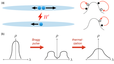
Figure 1: (a) Depiction of two tubes coupled by the perturbation $H^{\prime}$. The leading contribution to thermalization comes from collisions among three quasiparticles, which rearranges the rapidity distribution (sketched on the right side of the figure). (b) Schematic for the evolution of the rapidity distribution under the experimental protocol, which consists of a Bragg pulse followed by thermalization.

In the present work we address thermalization in such weakly coupled interacting integrable chains, initialized in arbitrary (but spatially uniform) nonequilibrium states. In this sense our work is complementary to the generalized hydrodynamics (GHD) program, which focuses on the relaxation of initially nonuniform states Castro-Alvaredo et al. (2016); Bertini et al. (2016); Bulchandani et al. (2018); Panfil and Pawełczyk (2019); Doyon (2020); Schemmer et al. (2019); Malvania et al. (2021); Møller et al. (2021). We study the dynamics of thermalization via the time-evolution of the quasiparticle rapidity distribution, which is experimentally measurable through time-of-flight experiments Wilson et al. (2020). The rapidity distribution evolves according to a Boltzmann equation, with a collision integral for which we develop an efficient, quantitatively accurate computational scheme. Finding such explicit collision integrals has been one of the persistent challenges in the study of nearly integrable models: collision integrals that are similar to the one we derive were previously proposed in the literature Caux et al. (2019); Friedman et al. (2020); Bastianello et al. (2020a, b); Durnin et al. (2021); Bastianello et al. (2021); Lopez-Piqueres et al. (2021); De Nardis et al. (2021), but have not been used to study relaxation from physically relevant nonequilibrium initial states. (For complementary approaches to the problem of weak integrability breaking see Refs. Bertini et al. (2015); Ristivojevic and Matveev (2016); Mallayya et al. (2019); Bulchandani et al. (2021); Pandey et al. (2020); Hutsalyuk and Pozsgay (2021); LeBlond et al. (2021).) Here, we apply our collision integral to characterize the relaxation of coupled Bose gases initialized in the experimentally relevant “Newton’s cradle” setup Kinoshita et al. (2006) (Fig. 1). In an (idealized) Newton’s cradle experiment, a gas is prepared in a low-temperature equilibrium state, and is then subjected to a pulse that boosts the momenta of half the atoms by $p$ and the other half by $-p$. When the dynamics is not exactly integrable Tang et al. (2018), this nonequilibrium state slowly relaxes to a higher-temperature equilibrium state (Fig. 1b).

Our main result is a quantitative description of how the quasiparticle distribution evolves during this relaxation process. From the quasiparticle distribution, we can also straightforwardly compute the evolution of charge and energy currents, and of the entire hierarchy of charges that are strictly conserved in the integrable limit Ilievski et al. (2015); Ilievski and De Nardis (2017). For the far-from-equilibrium initial state we focus on, this relaxation is a complex multiple-scale process that we can only solve numerically. However, assuming the system thermalizes, then at late times it is near equilibrium and one can linearize the Boltzmann equation. We present evidence that the spectrum of the resulting linear operator is gapless and spans several orders of magnitude. The late-time approach to equilibrium is thus not governed by a single characteristic timescale. This is true, remarkably, even though the initial state is spatially uniform, so the quench does not directly couple to any hydrodynamic-scale density fluctuations.

Model—We consider an array of one-dimensional bosonic gases (“tubes”), oriented along the $x$ axis, each governed by the Lieb-Liniger Hamiltonian

$$H_{\mathrm{LL},i}=\int dx\,\hat{\psi}_{i}^{\dagger}(x)\left[-\frac{1}{2m}\partial_{x}^{2}+c\hat{\rho}_{i}(x)\right]\hat{\psi}_{i}(x).$$ (1)

Here, $i$ indexes the tubes, $m$ is the microscopic mass of the bosons, $\hat{\rho}_{i}(x)\equiv\hat{\psi}^{\dagger}_{i}(x)\hat{\psi}_{i}(x)$ is the density operator, and $c$ is a coupling constant. The tubes are coupled to one another by density-density interactions of the form

$$H^{\prime}=V_{0}\sum_{ij}\int dxdx^{\prime}A_{ij}(|x-x^{\prime}|)\hat{\rho}_{i}(x)\hat{\rho}_{j}(x^{\prime}).$$ (2)

We will leave $A_{ij}(|x-x^{\prime}|)$ generic for now, but we are primarily interested in the case of dipole-dipole interactions, where $A_{ij}=(1-3\cos^{2}(\theta_{ij}))/(|x-x^{\prime}|^{2}+|\mathbf{r}_{i}-\mathbf{r}_{j}|^{2})^{3/2}$. Here, $\mathbf{r}_{i}\equiv(y_{i},z_{i})$ is the position of the $i$th tube in the array, and $\theta_{ij}$ is the angle between the separation $\mathbf{r}_{i}-\mathbf{r}_{j}$ and the orientation of the dipoles (which is fixed in the experiment by applying a magnetic field).

For simplicity we anticipate that $A_{ij}$ falls off fast enough with distance between tubes that it is sufficient to consider nearest-neighbor interactions between tubes. Thus each tube interacts with $z$ neighbors. With the Newton’s cradle experiment in mind, we also assume in what follows that the tubes have identical quasiparticle distributions in the nonequilibrium initial state. Under these assumptions, it suffices to consider the effects of the integrability-breaking perturbation acting on a pair of neighboring tubes; we thus drop the indices on the interaction shape $A(x)$.

Boltzmann equation for two tubes—We assume a separation of scales between the fast dynamics due to $H_{\mathrm{LL}}$ and slow dynamics due to $H^{\prime}$. Without loss of generality we pick tube 1 as the “system” tube (whose rapidity distribution is being measured) and tube 2 as a “bath” tube. On timescales that are long compared with the fast dynamics, the state of each tube can be characterized by a generalized Gibbs ensemble Ilievski et al. (2015); Caux and Konik (2012); Mossel and Caux (2012), or equivalently by its quasiparticle distribution function $\rho_{p}(\lambda)$, where $\lambda$ is the “rapidity”. The rapidity labels particles in interacting integrable models in an analogous way to momentum in free theories. The distribution $\rho_{p}(\lambda)$ evolves in general as

$$\partial_{t}\rho_{p,1}(\lambda)=\tau^{-1}Q[\rho_{p,1},\rho_{p,2}](\lambda).$$ (3)

We emphasize that the right-hand side (the so-called “collision integral”) is a nontrivial functional of the density distributions in the two tubes. For the present, we restrict to the case where the density distributions are initially identical, and thus stay identical at all times (at our level of analysis). The time scale for the evolution follows from the Fermi’s golden rule and is set by $\tau^{-1}\equiv 16E_{F}/(\hbar\pi^{2})\times\gamma_{\rm inter}^{2}$, where $E_{F}$ is the Fermi energy of the single tube and $\gamma_{\rm inter}\equiv V_{0}m/(n_{\rm 1D}\hbar^{2})$ is the dimensionless coupling between the two tubes with $n_{\rm 1D}$ the one-dimensional density of the gas. The full derivation of the collision integral, including the case of different distributions in the two tubes, is presented in the Supplemental Material, Section $2$. Here we discuss in details the ingredients of the resulting expression.

The population at rapidity $\lambda$ may change for two reasons: either because a particle directly scatters into or out of that rapidity, or indirectly due to interactions. (As an example, in a finite system, changing the rapidity of one particle alters the quantization condition for all the others, via the Bethe equations.) In the thermodynamic limit, this “backflow” effect can be taken into account through the relation $Q[\rho_{p}](\lambda)=\int d\mu R[\rho_{p}](\lambda,\mu)Q_{0}[\rho_{p}](\mu)$, where $Q_{0}$ is the direct scattering rate given by Fermi’s Golden Rule, and $R$ is an integral operator (which is purely a property of the integrable dynamics) that captures the influence of this scattering process elsewhere in rapidity-space, see . Henceforth we will drop the $\rho_{p}$ argument, noting that all quantities of interest are functionals of the full distribution. A physical choice of $Q_{0}$ must conserve particle number in each tube, as well as total momentum and energy in the full array. In our setup, since the tubes are identical, momentum and energy will be also conserved on ‘average’ (in a temporal sense) in each tube.

We now turn to computing $Q_{0}$. We write $Q_{0}=\sum_{n,m}Q_{0}^{(n,m)}$, where $Q_{0}^{(n,m)}$ is a scattering process involving $n$ particle-hole excitations in the system tube and $m$ particle-hole excitations in the bath tube. We can write $Q_{0}^{n,m}(\lambda)$ so that the focus is on the n-particle-hole excitations in the system tube. Let these be indexed by $\{(p_{i},h_{i})\}^{n}_{i=1}$. We want to consider all possible distinct particle-hole combinations such that the rapidity $\lambda$ is equal to $p_{i}$ or $h_{i}$ for some i. The scattering event, $\{(p_{i},h_{i})\}^{n}_{i=1}$, will change the system tube’s energy/momentum by $(\omega,k)$. By energy-momentum conservation the $m-$particle-hole process in the bath tube must change by $(-\omega,-k)$. The ability of the bath tube to support such an excitation complex is encoded in the spectral density of the bath tube, a quantity we denote as $S^{m}_{2}(k,\omega)$. The scattering processes in both tubes are governed by matrix elements of the density operator (as the interaction between tubes is density-density). We write the matrix element for the system tube as $F^{\rho_{1}}(\{p_{i},h_{i}\}^{m}_{i=1})=\langle\rho_{p}|\hat{\rho}_{1}(x)|\rho_{p};\{h_{i}\}\to\{p_{i}\}\rangle$. The contribution of the particle-hole combination $\{(p_{i},h_{i})\}^{n}_{i=1}$ in the system tube to $Q_{0}^{n,m}$ is controlled by the particle and hole densities, $\rho_{p1}$/$\rho_{h1}$ and so is proportional to $\prod_{i=1}^{n}\rho_{p_{1}}(h_{i})\rho_{h_{1}}(p_{i})$. Putting these features together allows us to write $Q_{0}^{n,m}$ as

$$Q^{(n,m)}_{0}(\lambda) = \frac{n}{(n!)^{2}}\int\prod_{i=1}^{n}dp_{i}dh_{i}\delta(\lambda-p_{1})A^{2}(k)\left|F^{\rho_{1}}(\{p_{i},h_{i}\})\right|^{2}\left[\rho_{p1}(h_{i})\rho_{h1}(p_{i})S_{2}^{m}(-k,-\omega)-({h_{i}}\leftrightarrow{p_{i}})\right].$$ (4)

We derive this form more concretely in .

To make further progress with Eq. (4) we must evaluate the $m$-particle-hole matrix elements $F^{\rho}$ and the $m$-particle-hole contribution to the dynamic structure factor. In general, processes with any $(n,m)$ contribute comparably to relaxation and one must sum over these processes, which is evidently intractable. However under the assumption that the intertube interactions are varying smoothly with the distance the relaxation is dominated by processes transferring small momenta. This implies that higher particle-hole processes that involve higher powers of the momentum transfer (see Appendix A), can be neglected. Another regime dominated by few-particle processes is the $c\to\infty$ (Tonks-Girardeau) limit in which processes involving $n-$particle-holes are suppressed by $c^{-2n}$.

The simplest interaction process is governed by $Q_{0}^{(1,1)}$, i.e., by two-particle scattering. However, the kinematics of one-dimensional two-body scattering is too restrictive to lead to thermalization; indeed, if the distributions in the two tubes are initially the same, $Q_{0}^{(1,1)}$ has no nontrivial dynamical effects. Thus, the leading processes that do contribute are $Q_{0}^{(1,2)}$ and $Q_{0}^{(2,1)}$: i.e., diffractive three-body scattering processes involving two particles in one tube and one in the other .

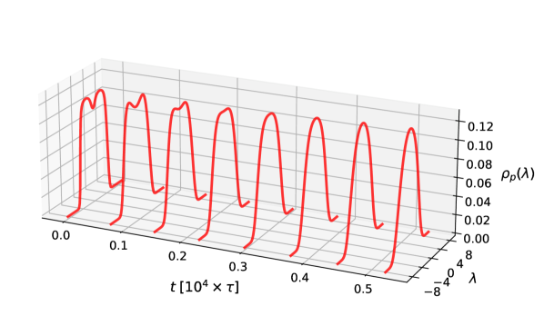
Figure 2: Evolution of the quasiparticle distribution in one of the tubes for the nonequilibrium protocol described in the main text. The evolution is characterized by a quick washing out of the two Bragg peaks followed by a relatively slower approach to the final equilibrium distribution, as further shown in Fig. 3(a).

The scattering rates $Q_{0}^{(1,2)}$ and $Q_{0}^{(2,1)}$ can be evaluated in the limit of small momentum transfer, using recently developed expressions for the form factors $F^{\rho}(p_{;}h)$ and $F^{\rho}(p_{1},p_{2};h_{1},h_{2})$ above a generalized Gibbs state Nardis and Panfil (2015, 2016); De Nardis and Panfil (2018); Nardis et al. (2019a); Cortés Cubero and Panfil (2019); Cortes Cubero and Panfil (2020); Panfil (2021). The dynamic structure factor can also be expressed in terms of these same form factors by means of a spectral representation Essler and Konik (2005). One of the challenges in employing form factors in computing the scattering rates and structure factors is to make sense of the non-integrable singularities they introduce Konik (2003); Essler and Konik (2009, 2008). In order to tackle this problem we use the Hadamard regularization , the method used earlier in computing response functions at finite energy density as well as in the context of diffusion in generalized hydrodynamics, Refs. Pozsgay and Takács, 2010; Nardis et al., 2019b; Cortés Cubero and Panfil, 2019; Panfil, 2021.

Results—

We study now in details the time evolution of the system prepared in the following initial state motivated by the recent experiments Tang et al. (2018). Initially, the two tubes are in thermal equilibrium at temperature $T_{0}$ and with the chemical potential $h_{0}$. The corresponding quasiparticle distribution is $\rho_{T_{0},h_{0}}(\lambda)$. We imagine now performing a Bragg pulse effectively boosting each cloud of atoms by $\pm p$ such that $\rho_{pi}(\lambda,0)=(\rho_{T_{0},h_{0}}(\lambda+p)+\rho_{T_{0},h_{0}}(\lambda-p))/2$. The system then evolves according to (3). As discussed above, for the distributions in both tubes are identical the leading processes are $(1,2)$ and $(2,1)$. To be specific we fix the interaction parameter $c=4$ which corresponds to a strongly correlated regime of the Lieb-Liniger model. For the initial state we choose system at $k_{B}T=1$ and unit density $n_{\rm 1D}=1$ and set $p=2.3$. In Fig. 2 we show the resulting time evolution and in Fig. 3(a) we compare the initial distribution and the distribution at late time. This clearly shows the thermalization with the thermal distribution fixed by the particle density and the energy right after the Bragg pulse. Additionally the thermalization process can be witnessed by observing the diagonal entropy production Polkovnikov (2011) as we discuss in more details in the Supplementary Material, Section S3).

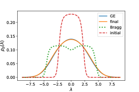
(a)

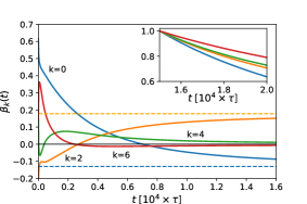
(b)

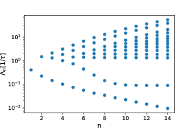
(c)

Figure 3: (a) Initial, post Bragg-pulse and final (at $t=2\times 10^{4}\tau$) quasiparticle distributions. The final distribution coincides with the thermal equilibrium distribution with $k_{B}T\approx 11.25$ fixed from the energy of the post Bragg-pulse state. (b) Evolution of the generalized chemical potentials $\beta_{k}(t)$ determining the ensemble of the gas as a function of time. We consider truncated GGE of ultra-local charges with first $4$ even charges. The dashed lines are the equilibrium values. In the inset we show that the thermalization rates for different chemical potentials are different. (c) The eigenvalues of the dimensionless linearized and truncated evolution operator $\bar{\mathbf{Q}}_{0}^{(1,2)}$ for the thermal state approached by nonequilibrium evolution and for different values of the truncation order $n$. To simplify the interpretation, while evaluating $\bar{\mathbf{Q}}_{0}^{(1,2)}$, we work in the large $c$ limit, where the dressings are subleading. All the eigenvalues are positive and the smallest and largest eigenvalues differ by few orders of magnitude. The smallest value monotonically decrease upon increasing the truncation order $n$ and conjecturally approaches zero.

The instantaneous states of the system can be described by the generalized Gibbs ensemble (GGE). The GGE involves, beside particle number and total energy, also all other local conserved charges $Q_{k}$ present in uncoupled Lieb-Liniger model. The GGE density matrix takes then the form $\hat{\rho}\sim\exp(-\sum_{k}\beta_{k}Q_{k})$. The distribution $\rho_{\rm p}(\lambda)$ is in one-to-one correspondence with the chemical potentials $\beta_{k}$ (see Appendix B). The dynamics of $\rho_{\rm p}(\lambda)$ can be then translated in the time dependence of the chemical potentials $\beta_{k}(t)$. This is a convenient way to explore thermalization: in the thermal state only $\beta_{0}$ and $\beta_{2}$ are not zero, so all other $\beta_{n}(t)$ should decay to zero. The initial distribution is an even function of the rapidity and the time evolution does not modify that and therefore only even chemical potentials are potentially non-zero. In Fig. 3(b) we plot first few chemical potentials. We observe that $\beta_{k}(t)$ for $k>2$ approach at large times zero signalling again the thermalization. In the inset we consider $(\beta_{k}(t)-\beta_{k}^{\rm th})$ for large times and normalized by the values at specific time $t^{*}$ such that each line starts at $1$. This shows that the system does not display a single timescale for thermalization. Instead the thermalization rate depends on the generalized chemical potential considered with the one corresponding to the particle number and energy evolving the slowest.

At very late times, we can assume the system is near a thermal state, allowing us to linearize the Boltzmann equation about the thermal state. The process of thermalization is then determined by the spectrum of the resulting linear operator $\mathbf{Q}_{0}$ . This operator further decomposes into contributions $\mathbf{Q}_{0}^{(n,m)}$ analogously to the full dynamics. The two leading processes $(1,2)$ and $(2,1)$ lead then to a symmetric operator $\bar{\mathbf{Q}}_{0}^{(1,2)}=\mathbf{Q}_{0}^{(1,2)}+\mathbf{Q}_{0}^{(2,1)}$ whose spectrum we now analyse.

The spectrum of this operator has three zero modes, corresponding to energy, particle number, and momentum conservation. The rate of approach to the steady state is set by the smallest-magnitude nonzero eigenvalue. To learn about its spectrum we truncate the infinite-dimensional operator $\bar{\mathbf{Q}}_{0}^{(1,2)}$ to a finite-dimensional space spanned by the lowest ultra local conserved charges not contained in its kernel. The spectrum of this truncated operator is plotted in Fig. 3(c) as a function of the truncation order. We find that the magnitude of the lowest nonzero eigenvalue rapidly decreases with increasing truncation order. Our numerical results suggest (though we cannot prove) that the operator is gapless: thus, there is a spectrum of relaxation times going all the way out to infinity, and the approach to the steady state is non-exponential. This feature is unexpected: usually, power-law relaxation in nonintegrable systems is associated with the hydrodynamics of long-wavelength density fluctuations, but the initial states we consider are translation-invariant and do not have such fluctuations. Understanding the origin of this gapless spectrum—and whether it is generic—is an interesting question for future work.

Summary—In this work we addressed a central challenge in the study of nearly integrable systems: we developed a Boltzmann equation with a microscopically derived collision integral, to describe the relaxation of the system to equilibrium. This Boltzmann equation is quantitatively accurate for perturbations that fall off slowly in space, e.g., dipolar interactions between integrable chains. This Boltzmann equation applies to arbitrary initial states, though for simplicity we assumed translation invariance. Our main result is that relaxation from the Newton’s cradle setup is a process that involves many different timescales: indeed, our numerical results on the linearized Boltzmann equation suggest that relaxation is non-exponential even at the latest times. An important future direction would be to extend our results to spatially inhomogeneous initial states and systems confined in harmonic traps: this would involve combining our Boltzmann equation (applied locally) with the nontrivial evolution of the quasiparticle distributions under generalized hydrodynamics, including space-time inhomogeneities Bastianello et al. (2019). In experimental setups the gas is confined in a 3D trap. This leads to a new integrability breaking perturbation through virtual excitations into higher radial modes Ristivojevic and Matveev (2016). In the case considered here where the dynamics are dominated by low momenta particle-hole excitations, virtual excitations involving higher radial modes are suppressed by a high power of momentum  Ristivojevic and Matveev (2016) and so presumably are subdominant. Nonetheless, it would be valuable to understand the effects of such integrability breaking on dynamics in more general scenarios. We are also interested in applying the formalism developed herein to the problem of thermalization in spin chain materials Scheie et al. (2021) including rare earth variants Wu et al. (2016); Gannon et al. (2019); Nikitin et al. (2020) placed out of equilibrium and probed by neutron and resonant inelastic x-ray scattering.

Acknowledgments— M.P. acknowledges the support from the National Science Centre, Poland, under the SONATA grant 2018/31/D/ST3/03588. S.G. acknowledges support from NSF DMR-1653271. R.M.K. was supported by the U.S. Department of Energy, Office of Basic Energy Sciences, under Contract No. DE-SC0012704.

Appendix A—

In this appendix we analyze the dependence of the scattering integral on the momentum $k$ transferred between the tubes. To this end, the integration over $(p_{i},h_{i})$ in (4) can be transformed into an integration over $(k_{i},\omega_{i})$ where

$$k_{i}=k(p_{i})-k(h_{i}),\qquad\omega_{i}=\omega(p_{i})-\omega(h_{i}).$$ (5)

The Jacobian of the $J$ transformation is

$$J^{-1}=\prod_{j=1}^{n}k^{\prime}(p_{i})k^{\prime}(h_{i})|v^{\rm eff}(p_{i})-v^{\rm eff}(h_{i})|.$$ (6)

We assume that in the small momentum limit the relevant excitations take the form of small particle-hole excitations, $p_{i}\sim h_{i}$. For small particle-hole excitations, we have that $J\sim\prod_{i=1}^{n}|k_{i}|^{-1}$. Therefore each integration over $k_{i}$ and $\omega_{i}$, including the presence of the Jacobian, gives a factor $k_{i}$ (we assume the energy is linear in $k_{i}$). The Dirac $\delta$-function reduces the number of integrals by one and effectively decreases the order in $k$ by $1$. Therefore, the phase space of the excitations scales like $k^{n-1}$.

We use now that the form-factors are, in the leading order, momentum independent and that for $\omega\sim k$, $S^{m}(k,\omega)\sim|k|^{m-2}$ Panfil (2021). Finally, because $\rho_{p1}(h_{i})\rho_{h1}(p_{i})-({h_{i}}\leftrightarrow{p_{i}})\sim k$, there is an additional power of $k$ coming from the particle-hole distributions. For symmetric potential $A(k)=A(-k)$ the leading term vanishes and collecting the factors we find $Q_{0}^{(n,m)}\sim k^{n+m-1}$.

Appendix B—

To read off the chemical potentials $\beta_{k}$ from a given distribution $\rho_{\rm p}(\lambda)$ we invert the usual procedure of computing the distribution from the knowledge of the chemical potentials Caux and Konik (2012). In practice we first compute $\rho_{\rm tot}(\lambda)$ from the defining integral equation Korepin et al. (1993),

$$\rho_{\rm tot}(\lambda)=\frac{1}{2\pi}+\!\int\!{\rm d}\mu\,T(\lambda-\mu)\rho_{\rm p}(\mu),\;T(\lambda)=\frac{c}{\pi}\frac{1}{\lambda^{2}+c^{2}}.$$ (7)

This gives us an access to the filling function $n(\lambda)=\rho_{\rm p}(\lambda)/\rho_{\rm tot}(\lambda)$. The filling function is expressed through the pseudo-energy $\epsilon(\lambda)$ as $n(\lambda)=[1+\exp(\epsilon(\lambda))]^{-1}$. The pseudo-energy itself is related to the bare pseudo-energy $\epsilon_{0}(\lambda)$ through the integral relation,

$$\epsilon(\lambda)=\epsilon_{0}(\lambda)-\int{\rm d}\mu\,T(\lambda-\mu)\log\left(1+e^{-\epsilon(\mu)}\right).$$ (8)

Finally, the bare pseudo-energy is expressed through the chemical potentials as $\epsilon_{0}(\lambda)=\sum_{k}\beta_{k}\lambda^{k}$, where $\lambda^{k}$ is the single particle contribution to the charge $Q_{k}$, namely

$$Q_{k}=\int{\rm d}\lambda\;\lambda^{k}\rho_{\rm p}(\lambda).$$ (9)

References

- D’Alessio et al. (2016) L. D’Alessio, Y. Kafri, A. Polkovnikov, and M. Rigol, Advances in Physics 65, 239 (2016).
- Takahashi (2005) M. Takahashi, Thermodynamics of One-Dimensional Solvable Models (2005).
- Rigol et al. (2008) M. Rigol, V. Dunjko, and M. Olshanii, Nature 452, 854 (2008).
- Ilievski et al. (2015) E. Ilievski, J. De Nardis, B. Wouters, J.-S. Caux, F. H. L. Essler, and T. Prosen, Phys. Rev. Lett. 115, 157201 (2015).
- Langen et al. (2015) T. Langen, S. Erne, R. Geiger, B. Rauer, T. Schweigler, M. Kuhnert, W. Rohringer, I. E. Mazets, T. Gasenzer, and J. Schmiedmayer, Science 348, 207 (2015).
- Tang et al. (2018) Y. Tang, W. Kao, K.-Y. Li, S. Seo, K. Mallayya, M. Rigol, S. Gopalakrishnan, and B. L. Lev, Phys. Rev. X 8, 021030 (2018).
- Kao et al. (2021) W. Kao, K.-Y. Li, K.-Y. Lin, S. Gopalakrishnan, and B. L. Lev, Science 371, 296 (2021).
- Scheie et al. (2021) A. Scheie, N. Sherman, M. Dupont, S. Nagler, M. Stone, G. Granroth, J. Moore, and D. Tennant, Nature Physics 17, 726 (2021).
- Castro-Alvaredo et al. (2016) O. A. Castro-Alvaredo, B. Doyon, and T. Yoshimura, Phys. Rev. X 6, 041065 (2016).
- Bertini et al. (2016) B. Bertini, M. Collura, J. De Nardis, and M. Fagotti, Phys. Rev. Lett. 117, 207201 (2016).
- Bulchandani et al. (2018) V. B. Bulchandani, R. Vasseur, C. Karrasch, and J. E. Moore, Phys. Rev. B 97, 045407 (2018).
- Panfil and Pawełczyk (2019) M. Panfil and J. Pawełczyk, SciPost Phys. Core 1, 002 (2019).
- Doyon (2020) B. Doyon, SciPost Physics Lecture Notes , 018 (2020).
- Schemmer et al. (2019) M. Schemmer, I. Bouchoule, B. Doyon, and J. Dubail, Phys. Rev. Lett. 122, 090601 (2019).
- Malvania et al. (2021) N. Malvania, Y. Zhang, Y. Le, J. Dubail, M. Rigol, and D. S. Weiss, Science 373, 1129 (2021).
- Møller et al. (2021) F. Møller, C. Li, I. Mazets, H.-P. Stimming, T. Zhou, Z. Zhu, X. Chen, and J. Schmiedmayer, Phys. Rev. Lett. 126, 090602 (2021).
- Wilson et al. (2020) J. M. Wilson, N. Malvania, Y. Le, Y. Zhang, M. Rigol, and D. S. Weiss, Science 367, 1461 (2020).
- Caux et al. (2019) J.-S. Caux, B. Doyon, J. Dubail, R. Konik, and T. Yoshimura, SciPost Physics 6, 070 (2019).
- Friedman et al. (2020) A. J. Friedman, S. Gopalakrishnan, and R. Vasseur, Phys. Rev. B 101, 180302 (2020).
- Bastianello et al. (2020a) A. Bastianello, J. De Nardis, and A. De Luca, Phys. Rev. B 102, 161110 (2020a).
- Bastianello et al. (2020b) A. Bastianello, A. De Luca, B. Doyon, and J. De Nardis, Phys. Rev. Lett. 125, 240604 (2020b).
- Durnin et al. (2021) J. Durnin, M. J. Bhaseen, and B. Doyon, Phys. Rev. Lett. 127, 130601 (2021).
- Bastianello et al. (2021) A. Bastianello, A. De Luca, and R. Vasseur, Journal of Statistical Mechanics: Theory and Experiment 2021, 114003 (2021).
- Lopez-Piqueres et al. (2021) J. Lopez-Piqueres, B. Ware, S. Gopalakrishnan, and R. Vasseur, Phys. Rev. B 103, L060302 (2021).
- De Nardis et al. (2021) J. De Nardis, S. Gopalakrishnan, R. Vasseur, and B. Ware, Phys. Rev. Lett. 127, 057201 (2021).
- Bertini et al. (2015) B. Bertini, F. H. L. Essler, S. Groha, and N. J. Robinson, Phys. Rev. Lett. 115, 180601 (2015).
- Ristivojevic and Matveev (2016) Z. Ristivojevic and K. A. Matveev, Phys. Rev. B 94, 024506 (2016).
- Mallayya et al. (2019) K. Mallayya, M. Rigol, and W. De Roeck, Phys. Rev. X 9, 021027 (2019).
- Bulchandani et al. (2021) V. B. Bulchandani, D. A. Huse, and S. Gopalakrishnan, “Onset of many-body quantum chaos due to breaking integrability,” (2021).
- Pandey et al. (2020) M. Pandey, P. W. Claeys, D. K. Campbell, A. Polkovnikov, and D. Sels, Phys. Rev. X 10, 041017 (2020).
- Hutsalyuk and Pozsgay (2021) A. Hutsalyuk and B. Pozsgay, Phys. Rev. E 103, 042121 (2021), arXiv:2012.15640 [cond-mat.quant-gas] .
- LeBlond et al. (2021) T. LeBlond, D. Sels, A. Polkovnikov, and M. Rigol, Phys. Rev. B 104, L201117 (2021).
- Kinoshita et al. (2006) T. Kinoshita, T. Wenger, and D. S. Weiss, Nature 440, 900 (2006).
- Ilievski and De Nardis (2017) E. Ilievski and J. De Nardis, Phys. Rev. Lett. 119, 020602 (2017).
- Caux and Konik (2012) J.-S. Caux and R. M. Konik, Phys. Rev. Lett. 109, 175301 (2012), arXiv:1203.0901 [cond-mat.quant-gas] .
- Mossel and Caux (2012) J. Mossel and J.-S. Caux, J. Phys. A: Math. Theor. 45, 255001 (2012).
- Note (1) Please see Section S2 of the Supplementary Material.
- Note (2) Please see Section S2.2-S2.3 of the Supplementary Material.
- Note (3) These two processes are physically different: in , the quasiparticle with rapidity scatters to a new state while causing a two-particle rearrangement in the other tube; in this quasiparticle is involved in a two-body scattering process.
- Nardis and Panfil (2015) J. D. Nardis and M. Panfil, J. Stat. Mech. Theor. Exp. 2015, P02019 (2015).
- Nardis and Panfil (2016) J. D. Nardis and M. Panfil, SciPost Phys. 1, 015 (2016).
- De Nardis and Panfil (2018) J. De Nardis and M. Panfil, Journal of Statistical Mechanics: Theory and Experiment 3, 033102 (2018), arXiv:1712.06581 [cond-mat.quant-gas] .
- Nardis et al. (2019a) J. D. Nardis, D. Bernard, and B. Doyon, SciPost Phys. 6, 49 (2019a).
- Cortés Cubero and Panfil (2019) A. Cortés Cubero and M. Panfil, Journal of High Energy Physics 2019, 104 (2019), arXiv:1809.02044 [hep-th] .
- Cortes Cubero and Panfil (2020) A. Cortes Cubero and M. Panfil, SciPost Physics 8, 004 (2020).
- Panfil (2021) M. Panfil, Journal of Statistical Mechanics: Theory and Experiment 2021, 013108 (2021).
- Essler and Konik (2005) F. H. L. Essler and R. M. Konik, in From Fields to Strings: Circumnavigating Theoretical Physics (World Scientific, 2005) pp. 684–830.
- Konik (2003) R. M. Konik, Phys. Rev. B 68, 104435 (2003).
- Essler and Konik (2009) F. H. L. Essler and R. M. Konik, Journal of Statistical Mechanics: Theory and Experiment 2009, P09018 (2009).
- Essler and Konik (2008) F. H. L. Essler and R. M. Konik, Phys. Rev. B 78, 100403 (2008).
- Note (4) Please see Section S5 of the Supplementary Material.
- Pozsgay and Takács (2010) B. Pozsgay and G. Takács, Journal of Statistical Mechanics: Theory and Experiment 2010, P11012 (2010).
- Nardis et al. (2019b) J. D. Nardis, D. Bernard, and B. Doyon, SciPost Physics 6 (2019b), 10.21468/scipostphys.6.4.049.
- Polkovnikov (2011) A. Polkovnikov, Annals of Physics 326, 486 (2011), arXiv:0806.2862 [cond-mat.stat-mech] .
- Note (5) Please see Section S4 of the Supplementary Material.
- Bastianello et al. (2019) A. Bastianello, V. Alba, and J.-S. Caux, Phys. Rev. Lett. 123, 130602 (2019).
- Wu et al. (2016) L. S. Wu, W. J. Gannon, I. A. Zaliznyak, A. M. Tsvelik, M. Brockmann, J.-S. Caux, M. S. Kim, Y. Qiu, J. R. D. Copley, G. Ehlers, A. Podlesnyak, and M. C. Aronson, Science 352, 1206 (2016).
- Gannon et al. (2019) W. J. Gannon, I. A. Zaliznyak, L. S. Wu, A. E. Feiguin, A. M. Tsvelik, F. Demmel, Y. Qiu, J. R. D. Copley, M. S. Kim, and M. C. Aronson, Nature Communications 10 (2019), 10.1038/s41467-019-08715-y.
- Nikitin et al. (2020) S. E. Nikitin, T. Xie, A. Podlesnyak, and I. A. Zaliznyak, Phys. Rev. B 101, 245150 (2020).
- Korepin et al. (1993) V. E. Korepin, N. M. Bogoliubov, and A. G. Izergin, Quantum Inverse Scattering Method and Correlation Functions, Cambridge Monographs on Mathematical Physics (Cambridge University Press, 1993).