In-medium polarization tensor in strong magnetic fields (II):
Axial Ward identity at finite temperature and density

Abstract

We investigate the axial Ward identity (AWI) for massive fermions in strong magnetic fields. The divergence of the axial-vector current is computed at finite temperature and/or density with the help of a relation between the polarization and anomaly diagrams in the effective (1+1) dimensions realized in the lowest Landau level (LLL). We discuss delicate interplay between the vacuum and medium contributions that determines patterns of the spectral flow in the adiabatic limit and, more generally, the diabatic chirality production rate. We also establish an explicit relation between the AWIs from the LLL approximation and from the familiar triangle diagrams in the naive perturbative series with respect to the coupling constant.

I Introduction

In this series of papers, we investigate the polarization effects of the medium particles at finite temperature and/or density as well as of the vacuum fluctuations in strong magnetic fields. In the first paper Hattori and Itakura (2022), which is referred to as Paper I, we have provided the explicit forms of the vacuum and medium contributions to the one-loop polarization tensor in the lowest Landau level (LLL) approximation and discussed magneto-birefringence as a physical application, that is, the polarization-dependent photon dispersion relation induced by the strong magnetic fields. We have inspected delicate interplay between the vacuum and medium contributions.

In the second paper of the series, we discuss another application of the polarization tensor to the axial-charge generation. Although the polarization tensor is a current correlator of the vector-vector type, one can apply it to the induction of the axial-vector current because there is an identity between the vector and axial-vector currents expanded with the eigenstates of the Landau levels. This identity is an analogue of that in the (1+1)-dimensional QED and the physical reason behind this identity is the chirality-momentum locking in the spin eigenstates (see Sec. II for more details).

Mechanisms of the axial-charge generation have attracted much attention over the last decade since a nonzero axial charge implies a parity-odd environment and induces transport phenomena that do not occur in parity-even environments. One of the prominent examples is induction of an electric current in magnetic fields, which is known as the chiral magnetic effect (CME) Kharzeev et al. (2008); Fukushima et al. (2008). The anomalous transport phenomena have been intensively investigated in the contexts of quark-gluon plasma created by relativistic heavy-ion collisions Kharzeev et al. (2016); Skokov et al. (2017); Hattori and Huang (2017) and of the Weyl and Dirac semimetals in condensed matter physics Burkov (2015); Gorbar et al. (2018); Armitage et al. (2018). The chiral magnetic effect, together with Ampère’s law, further implies an exponential growth of the magnetic-field strength driven by a positive feedback cycle when the magnetic field is lifted to a dynamical field. This is called the chiral plasma instability Akamatsu and Yamamoto (2013) and is expected to be possible mechanisms for generation of the strong magnetic fields during supernova explosions Yamamoto (2016); Yamamoto and Yang (2020) and of the primordial magnetic field in the early universe Turner and Widrow (1988); Carroll et al. (1990); Garretson et al. (1992); Joyce and Shaposhnikov (1997); Giovannini (2004); Laine (2005). Those hot situations, including the very recent CME search by isobaric collisions Abdallah et al. (2022), motivate us to investigate the axial-charge generation. Although the CME conductivity is given by a universal form stemming from chiral anomaly, it is also proportional to the magnitude of the axial chemical potential that is a thermodynamic conjugate quantity to the axial-charge density and depends on dynamics in individual systems. To name a few, the axial-charge dynamics was investigated in Refs. Tanji et al. (2016); Mueller et al. (2016); Hou and Lin (2018); Tanji (2018); Copinger et al. (2018); Taya (2020); Müller and Yang (2022); Yang (2021) for relativistic heavy-ion collisions, Refs. Grabowska et al. (2015); Gorbar and Shovkovy (2021) for neutron-star physics, and Refs. Domcke et al. (2020); Boyarsky et al. (2021) for cosmology.

We investigate the axial-charge generation from a fundamental point of view in terms of the divergence of the axial-vector current. QED contains chiral anomaly Adler (1969); Bell and Jackiw (1969), giving rise to the anomalous nonvanishing term in the divergence of the axial-vector current. A finite fermion mass explicitly breaks the chiral symmetry, and gives rise to another nonvanishing term in the divergence of the current. In case of (3+1)-dimensional QED, the well-known triangle diagrams yield both of those two nonvanishing contributions when the loop diagrams are composed of massive fermions.

There is, however, a significant difference between those two pieces of the same diagrams. The anomalous term does not receive radiative corrections Adler and Bardeen (1969); The anomalous term stems from the (superficial) ultraviolet divergence of the triangle diagrams, so that, without modifications of the divergent pole, there is no correction to the anomalous term. This means that there is no correction from the fermion mass or other external parameters such as temperature or density that do not modify the divergent pole Itoyama and Mueller (1983). In contrast, the mass-dependent part does not involve an ultraviolet divergence and can come with temperature and/or density corrections. The whole non-conservation equation of the axial-vector current, which we call the axial Ward identity (AWI), is controlled by the balance between the anomalous and mass-dependent terms that arise from the divergent and finite pieces of the loop integral.

Since the mass-dependent part in the AWI is not anomalous in nature, it does not exhibit simple behaviors in general when one varies magnitudes of relevant parameters such as the external photon momenta, fermion mass, temperature and/or density. Therefore, the AWI as a whole is not simply governed by the anomalous term and, moreover, the two terms can be comparable in magnitude, implying that the axial-vector current could be effectively conserved in some parameter regimes. Thus, we investigate the whole AWI with explicit computations.

Relevant processes for the axial-charge generation can be classified into adiabatic and diabatic processes according to the magnitude of energy transfer from the external photon fields (see Sec. IV.1 for a more precise definition). The adiabatic processes can be understood as the spectral flow that is a collective flow of the occupied states along the fermion dispersion relation Nielsen and Ninomiya (1983); Ambjorn et al. (1983) (see also Ref. Creutz (2001) for a review). The adiabatic flows occur when there is no energy transfer from the photon fields to the fermions and are only the processes for which one can get simple results. One should notice that the spectral flow occurs on the thermally occupied positive-energy states as well as on the negative-energy states beneath the Dirac sea, and induces the helicity flip at the bottom of the parabolic dispersion relation for massive fermions. In the other cases, i.e., the diabatic processes, nonzero energy transfer can induce intricate excitations that ruin the ordered collective flows. Such information is all encoded in the mass-dependent part. We provide a more detailed summary of the results in Sec. IV.1.

Incidentally, we also explicitly show a connection between the AWIs from the triangle diagrams and from the polarization tensor in the LLL approximation. Chiral anomaly is often explained as a product of the (1+1)-dimensional chiral anomaly and the Landau degeneracy factor on the basis of the effective dimensional reduction in the LLL Nielsen and Ninomiya (1983). The explicit computation of the LLL contribution, however, does not exactly reproduce the result from the triangle diagrams due to an extra Gaussian factor that stems from the fermion wave function in the LLL. This is simply because the wave function of the LLL fermion is not exactly (1+1) dimensional one, but has an extension in perpendicular to the magnetic field. The Gaussian factor reduces to unity in the homogeneous electric-field limit and/or the strong magnetic field limit such that the electric field does not resolve the transverse extension of the cyclotron orbits. As for the mass-dependent part, the LLL approximation reproduces that from the triangle diagrams when the constant magnetic field limit is taken for the triangle diagrams, again up to the Gaussian factor.

This paper is organized as follows. In Sec. II, we provide basic formulas for the induction of the vector and axial-vector currents by a single two-point correlator in the LLL approximation. In Sec. III, we summarize the explicit expressions of the polarization tensor from Paper I for readers’ convenience. Then, we discuss the AWI in detail in Sec. IV. In appendices, we clarify the quantum numbers characterizing the fermions in the LLL and perform an explicit computation of the divergence of the axial current composed of a massive Dirac fermion in the LLL, reproducing the expression from the polarization tensor. Finally, we discuss a connection between the AWIs computed from the LLL approximation and the triangle diagrams in Appendix C.

As in Paper I, we focus on a single-flavor Dirac fermion with an electric charge $q_{f}$ for simplicity, and introduce a single chemical potential conjugate to its number density. We also assume that a constant magnetic field is applied along the third spatial direction without loosing generality, i.e., ${\bm{B}}=(0,0,B)$. Accordingly, we use metric conventions $g^{\mu\nu}={\rm diag}(1,-1,-1,-1)$, $g_{\parallel}^{\mu\nu}={\rm diag}(1,0,0,-1)$, and $g_{\perp}^{\mu\nu}=(0,-1,-1,0)$ and associated notations $q_{\parallel}^{2}:=q_{\mu}q_{\nu}g_{\parallel}^{\mu\nu}$ and $q_{\perp}^{2}:=q_{\mu}q_{\nu}g_{\perp}^{\mu\nu}=-|{\bm{q}}_{\perp}|^{2}$ for four vectors $q^{\mu}$.

II Vector and axial Ward identities

The retarded polarization tensor serves as a linear response function with respect to electromagnetic perturbations. In this paper, we discuss induction of the currents transported by the LLL fermions

$$j_{V}^{\mu} = q_{f}\bar{\psi}_{\rm LLL}\gamma^{\mu}\psi_{\rm LLL}\,,$$ (1a)

$$j_{A}^{\mu} = \bar{\psi}_{\rm LLL}\gamma^{\mu}\gamma^{5}\psi_{\rm LLL}\,.$$ (1b)

The fermion spinor $\psi_{\rm LLL}$ in the LLL is an eigenstate of the spin projection operator ${\mathcal{P}}_{+}=(1+is_{f}\gamma^{1}\gamma^{2})/2$ with the sign function $s_{f}={\rm sgn}(q_{f}B)$. By the use of an identity among the gamma matrices $\gamma_{\parallel}^{\mu}\gamma^{5}{\mathcal{P}}_{\pm}=\mp s_{f}\epsilon_{\parallel}^{\mu\nu}\gamma_{\parallel\nu}{\mathcal{P}}_{\pm}$, we find a relation between the LLL contributions to the vector and axial-vector currents along the magnetic field

$$q_{f}j_{A}^{\mu}=-s_{f}\epsilon_{\parallel}^{\mu\nu}j_{V\nu}\,,$$ (2)

where we introduced an antisymmetric tensor $\epsilon_{\parallel}^{\mu\nu}$ which only has two non-vanishing components, $\epsilon_{\parallel}^{03}=-\epsilon_{\parallel}^{30}=1$. This relation is an analogue of the well-known relation in the (1+1) dimensional QED (see, e.g., a standard textbook Peskin and Schroeder (1995)) and is understood as a consequence of the effective dimensional reduction. Equation (2) relates the vector–vector (VV) correlator $\Pi^{\mu\nu}_{R}$, that we inspected in Paper I, to the vector–axial-vector (VA) correlator

$$\langle j_{A}^{\mu}j_{V}^{\nu}\rangle_{R}=-s_{f}\epsilon_{\parallel\,\rho}^{\mu}q_{f}^{-1}\Pi^{\rho\nu}_{R}\,.$$ (3)

The above vector and axial-vector currents are induced in response to an external $U(1)$ gauge field $A^{\mu}$. This is an external gauge field with an arbitrary frequency and wavelength, superimposed on top of the constant magnetic field. When the polarization tensor has a gauge-invariant tensor structure [see Eq. (5)], the vector and axial Ward identities read

$${\rm F.T.}\ \partial_{\mu}j_{V}^{\mu}=-iq_{\mu}\Pi^{\mu\nu}_{R}A_{\nu}=0\,,$$ (4a)

$${\rm F.T.}\ \partial_{\mu}j_{A}^{\mu}=-iq_{\mu}\langle j_{A}^{\mu}j_{V}^{\nu}\rangle_{R}A_{\nu}=s_{f}q_{f}^{-1}\Pi_{\parallel}\tilde{E}_{\parallel}(q)\,,$$ (4b)

where F.T. stands for the Fourier transform and $\tilde{E}_{\parallel}(q)=-i\epsilon_{\parallel}^{\mu\nu}q_{\mu}A_{\nu}$ is the parallel (or antiparallel) component of an electric field along the magnetic field. We put tilde on the electric field to emphasize that it is the Fourier spectrum, while the magnetic field $B$ (and ${\bm{B}}$ appearing below) is the constant magnitude throughout this paper. The vector Ward identity (4a) is a consequence of the gauge invariance in QED. However, the axial current is not conserved if the right-hand side in Eq. (4b) is nonzero. The magnitude of the nonvanishing divergence is controlled by the scalar function $\Pi_{\parallel}$ from the polarization tensor. In the next section, we provide the explicit form of $\Pi_{\parallel}$ from the vacuum and medium contributions.

III Polarization tensor

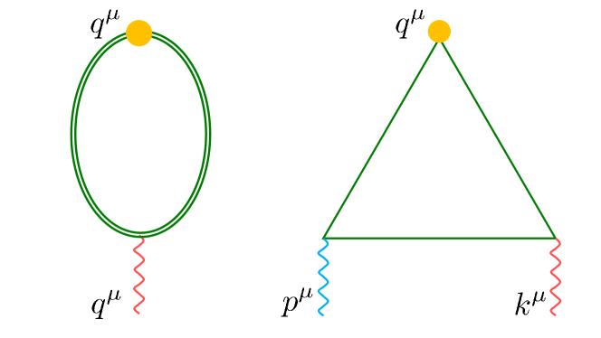
Figure 1: One-loop polarization tensor in strong magnetic fields [left] and the triangle diagram (with an exchange diagram not shown) [right]. The double lines show the fermion propagators in the LLL approximation that have insertions of the magnetic-field lines (not shown).

In Paper I, we provided detailed accounts on the computation of the polarization tensor in the LLL approximation (cf. the left panel in Fig. 1). Here, we briefly summarize its explicit form for readers’ convenience.

In the LLL approximation, one obtains the polarization tensor

$$\Pi^{\mu\nu}=m_{B}^{2}e^{-\frac{|{\bm{q}}_{\perp}|^{2}}{2|q_{f}B|}}\tilde{\Pi}_{\parallel}{\mathcal{P}}_{\parallel}^{\mu\nu}\,,$$ (5)

where $m_{B}^{2}=|q_{f}B|/(2\pi)\cdot q_{f}^{2}/\pi$. The gauge-invariant tensor structure is given as

$${\mathcal{P}}_{\parallel}^{\mu\nu}=g^{\mu\nu}_{\parallel}-\frac{q_{\parallel}^{\mu}q_{\parallel}^{\nu}}{q_{\parallel}^{2}}\,,$$ (6)

with the photon momentum $q^{\mu}$. Note that this tensor structure cannot be split into the longitudinal and transverse components with respect to the spatial photon momentum, because of its dimensionally reduced form. Therefore, this is the unique gauge-invariant tensor structure within the LLL approximation. There are some other tensor structures when the higher Landau levels contribute (see, e.g., Refs. Hattori and Itakura (2013); Hattori and Satow (2018)). The polarization function $\tilde{\Pi}_{\parallel}$ contains both the vacuum and medium contributions

$$\tilde{\Pi}_{\parallel}=\tilde{\Pi}_{\parallel}^{\rm vac}(q_{\parallel}^{2})+\tilde{\Pi}_{\parallel}^{\rm med}(\omega,q_{z})\,.$$ (7)

The medium contribution $\tilde{\Pi}_{\parallel}^{\rm med}(\omega,q_{z})$ depends on the photon energy $\omega$ and momentum $q_{z}$ separately, because the presence of medium breaks the Lorentz-boost invariance. Note also that we apply a constant magnetic field ${\bm{B}}$ in the medium rest frame. Configurations composed of constant magnetic fields in other Lorentz frames are not equivalent to the present configuration.

The explicit diagram computation provides the vacuum contribution (see the appendix in Paper I)

$$\tilde{\Pi}_{\parallel}^{\rm vac}(q_{\parallel}^{2})=1-I\big{(}\frac{q_{\parallel}^{2}}{4m^{2}}\big{)}\,.$$ (8)

Since the overall factor of $m_{B}^{2}$ is a dimension-two quantity in Eq. (5), the $I$ function can only be a function of a dimensionless variable:

$$I(x+i\omega\epsilon)=\left\{\begin{array}[]{ll}\frac{1}{2}\frac{1}{\sqrt{x(x-1)}}\ln\frac{\sqrt{x(x-1)}-x}{\sqrt{x(x-1)}+x}&x<0\\ \frac{1}{\sqrt{x(1-x)}}\arctan\frac{x}{\sqrt{x(1-x)}}&0\leq x<1\\ \frac{1}{2}\frac{1}{\sqrt{x(x-1)}}\left[\,\ln\frac{x-\sqrt{x(x-1)}}{x+\sqrt{x(x-1)}}+i\,{\rm sgn}(\omega)\pi\,\right]&1\leq x\end{array}\right.\,.$$ (12)

We took the retarded prescription $\omega\to\omega+i\epsilon$ that yields an infinitesimal displacement $q_{\parallel}^{2}\to q_{\parallel}^{2}+i\omega\epsilon$. The advanced and causal correlators can be computed in the same manner. One can find two limiting behaviors

$$I(0)=1\,,\quad I(\infty)=0\,.$$ (13)

Therefore, in the infinite-mass limit $q_{\parallel}^{2}/m^{2}\to 0$, we simply find that $\tilde{\Pi}_{\parallel}^{\rm vac}\to 0$ because the fermion excitations are suppressed. In the massless limit $q_{\parallel}^{2}/m^{2}\to\infty$, we have

$$\tilde{\Pi}_{\parallel}^{\rm vac}(q_{\parallel}^{2}) = 1\,.$$ (14)

The factor of $|q_{f}B|/(2\pi)$ in $m_{B}^{2}$ is called the Landau degeneracy factor. The remaining factor $q_{f}^{2}/\pi$ is known as the Schwinger mass in the (1+1) dimensional massless QED Schwinger (1962a, b) that provides a photon mass in the gauge-invariant way.

The medium contribution is obtained as (see Ref. Fukushima et al. (2016) and Paper I)

$$\tilde{\Pi}_{\parallel}^{{\rm med}}(\omega,q_{z})=\pi m^{2}\!\!\int_{-\infty}^{\infty}\frac{dp_{z}}{2\pi\epsilon_{p}}\frac{(q_{\parallel}^{2}+2q_{z}p_{z})\,[n_{+}(\epsilon_{p})+n_{-}(\epsilon_{p})]}{q_{\parallel}^{2}(p_{z}-\frac{1}{2}q_{z})^{2}-\frac{\omega^{2}}{4}(q_{\parallel}^{2}-4m^{2})}\,,$$ (15)

where the fermion energy and distribution function are given as $\epsilon_{p}=\sqrt{p_{z}^{2}+m^{2}}$ and $n_{\pm}(\epsilon_{p})=[e^{(\epsilon_{p}\mp\mu)/T}+1]^{-1}$, respectively. Notice that the medium contribution is proportional to the fermion mass and does not exist in the strictly massless case. The integrand has two poles at

$$p^{\pm}_{z}:=\frac{1}{2}\big{(}\,q_{z}\pm\omega\sqrt{1-4m^{2}/q_{\parallel}^{2}}\ \big{)}\,.$$ (16)

Thus, the integrand in Eq. (15) can be rearranged as

$$\tilde{\Pi}_{\parallel}^{{\rm med}}(\omega,q_{z})=\frac{2\pi m^{2}}{q_{\parallel}^{2}\sqrt{1-4m^{2}/q_{\parallel}^{2}}}\int_{-\infty}^{\infty}\frac{dp_{z}}{2\pi\epsilon_{p}}[n_{+}(\epsilon_{p})+n_{-}(\epsilon_{p})]\Big{(}\frac{\epsilon_{p}^{+}s_{+}}{p_{z}-p_{z}^{+}}-\frac{\epsilon_{p}^{-}s_{-}}{p_{z}-p_{z}^{-}}\Big{)}\,,$$ (17)

where we defined

$$s_{\pm}={\rm sgn}\Big{(}\omega\pm q_{z}\sqrt{1-4m^{2}/q_{\parallel}^{2}}\Big{)}={\rm sgn}(\omega)\,\theta(q_{\parallel}^{2}-4m^{2})\pm\theta(-q_{\parallel}^{2})\,,$$ (18a)

$$\epsilon_{p}^{\pm}=\sqrt{(p^{\pm}_{z})^{2}+m^{2}}=\frac{1}{2}\Big{|}\omega\pm q_{z}\sqrt{1-4m^{2}/q_{\parallel}^{2}}\ \Big{|}\,,$$ (18b)

for $1-4m^{2}/q_{\parallel}^{2}\geq 0$ and

$$s_{\pm}=1\,,$$ (19a)

$$\epsilon_{p}^{\pm}=\frac{1}{2}\Big{(}\omega\pm iq_{z}\sqrt{|1-4m^{2}/q_{\parallel}^{2}|}\ \Big{)}\,,$$ (19b)

for $1-4m^{2}/q_{\parallel}^{2}<0$.

Lastly, we give some comments on the imaginary part of the polarization tensor. The imaginary part in Eq. (12) indicates occurrence of a fermion-antifermion pair creation when the photon momentum satisfies the threshold condition $q_{\parallel}^{2}\geq(2m)^{2}$ that is the invariant mass of a pair in the LLL states (cf. Paper I). In the massless limit (14), an imaginary part only comes from the $q_{\parallel}^{2}$ pole in Eq. (6). The imaginary part is thus proportional to $\delta(q_{\parallel}^{2})$, meaning that there is no invariant energy transfer from a photon to a fermion-antifermion pair. Such a pair creation does not usually happen in (3+1) dimensions since a hole state in the Dirac sea needs to be created by a diabatic transition of a particle from the negative- to positive-energy branches. The pair creation in an adiabatic process can occur only because the positive- and negative-energy states are directly connected with each other in the (1+1)-dimensional gapless dispersion relation. Namely, the massless pair creation here can be interpreted as the spectral flow along the linear dispersion relation that occurs independently in the right- and left-handed sectors, leading to chiral anomaly. There is no medium correction in the massless case. The medium contribution (17) acquires imaginary parts in the massive case when the fermion and antifermion pair takes the energy $\epsilon_{p}^{\pm}$ and momentum $p^{\pm}_{z}$ as we inspected in Paper I. The created massive pairs posses nonzero axial charges.

IV Axial Ward identity in strong magnetic fields

IV.1 Summary of the results

In the following, we find that the AWI (4b) takes various forms depending on the scalar function $\Pi_{\parallel}$ stemming from the polarization tensor. Such behaviors crucially depend on whether fermions are massive or massless and whether there is the medium contribution or not. We provide summary of the characteristic behaviors before going into detailed discussions. The reasons/interpretations leading to those results are given in the following subsections.

In the strictly massless case, it is well-known that the divergence of the axial current is saturated by the anomalous term proportional to the pseudoscalar inner product of the electromagnetic field. It is thus useful to take this case as a reference result to other limits. Inserting the polarization tensor (14) into Eq. (4b), one finds the AWI

$${\rm F.T.}\ \partial_{\mu}j_{A}^{\mu}=s_{f}\rho_{B}\frac{q_{f}}{\pi}\tilde{E}_{\parallel}(q)\,e^{-\frac{|{\bm{q}}_{\perp}|^{2}}{2|q_{f}B|}}=\frac{q_{f}^{2}}{2\pi^{2}}\tilde{\bm{E}}(q)\cdot{\bm{B}}\,e^{-\frac{|{\bm{q}}_{\perp}|^{2}}{2|q_{f}B|}}\,.$$ (20)

Remember that $\tilde{E}_{\parallel}$ is the component of the electric field automatically projected in the magnetic-field direction in Eq. (4b) and depends on $q^{2}_{\parallel}$ and $|{\bm{q}}_{\perp}|^{2}$ in general, while $B$ is a constant strength. The same structure arises repeatedly below. This AWI (20) reproduces the chiral anomaly in the (3+1) dimensions up to the Gaussian factor. We will discuss the Gaussian factor below and put it aside at this moment.

Notice that both the divergence of the axial current and the product of the electromagnetic fields are dimension-four quantities. Therefore, the remaining factor in Eq. (20) is just a constant which is sometimes referred to as the anomaly coefficient. The same applies to the general form of $\Pi_{\parallel}$ in Eq. (4b). Since $\Pi_{\parallel}$ always has the overall factor of $q_{f}B$ from the Landau degeneracy factor, the remaining part has to be only a function of dimensionless quantities. Including all the contributions to $\Pi_{\parallel}$ obtained in Eq. (17), we find that

$${\rm F.T.}\ \partial_{\mu}j_{A}^{\mu}=w(\omega,q_{z})\frac{q_{f}^{2}}{2\pi^{2}}\tilde{\bm{E}}(q)\cdot{\bm{B}}\,e^{-\frac{|{\bm{q}}_{\perp}|^{2}}{2|q_{f}B|}}\,,$$ (21a)

$$w(\omega,q_{z}):=1-I\big{(}\frac{q_{\parallel}^{2}}{4m^{2}}\big{)}+m^{2}\int_{-\infty}^{\infty}\frac{dp_{z}}{\epsilon_{p}}\frac{n_{+}(\epsilon_{p})+n_{-}(\epsilon_{p})}{q_{\parallel}^{2}\sqrt{1-4m^{2}/q_{\parallel}^{2}}}\Big{(}\frac{\epsilon_{p}^{+}s_{+}}{p_{z}-p_{z}^{+}}-\frac{\epsilon_{p}^{-}s_{-}}{p_{z}-p_{z}^{-}}\Big{)}\,.$$ (21b)

The first term in $w(\omega,q_{z})$ is the same anomalous term as in the massless case (20), so that a deviation of $w(\omega,q_{z})$ from unity quantifies both the vacuum and medium contributions for massive fermions. It may be appropriate to call Eq. (21) the axial Ward identity (AWI) rather than the anomaly equation or something of this sort, because the right-hand side now has the terms other than the anomalous term. Those additional terms are identified with matrix elements of the pseudoscalar condensate, i.e., $2im\langle\bar{\psi}\gamma^{5}\psi\rangle$. In Appendix B, we confirm this statement with an explicit computation of the axial-vector correlator.

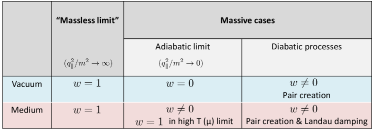
Figure 2: Summary of the limiting behaviors of $w(\omega,q_{z})$ that show relative magnitudes to the anomalous term. The high-$T$ limit refers to $m/T\to 0$ and $T/\mu\gg 1$, while the high-$\mu$ limit $m/\mu\to 0$ and $T/\mu\ll 1$.

We summarize the limiting behaviors defined by the dimensionless combinations below and in Table 2.

• “Massless” limit $q_{\parallel}^{2}/m^{2}\to\infty$: There is no medium correction in this limit, and the result is the same as in vacuum with massless fermions. This limit needs to be defined with a finite value of $q_{\parallel}^{2}$ that requires a nonzero energy $\omega$ and/or momentum $q_{z}$ of the electric field $\tilde{E}_{\parallel}$ along the magnetic-field direction. The absence of temperature corrections to the anomalous term was shown in the strictly massless case to all orders in the coupling constant Itoyama and Mueller (1983).

• Adiabatic limit $q_{\parallel}^{2}/m^{2}\to 0$ in vacuum: As explicitly shown in Sec. C, this limit corresponds to constant electric fields. The axial current is conserved in vacuum since a massive fermion and antifermion pair cannot be created in an adiabatic process Ambjorn et al. (1983).

• Adiabatic limit $q_{\parallel}^{2}/m^{2}\to 0$ in medium: The spectral flow occurs to the medium particles and gives rise to a nonzero divergence of the axial current. This is because acceleration by electric fields induces a momentum flip and thus a helicity flip when the spectral flow goes through the bottom of the parabolic dispersion relation. We will find that, in the high-temperature or density limit ($m/T,\ m/\mu\to 0$), the nonzero divergence takes the same form as the anomalous term in vacuum, though it arises from the mass-dependent part instead of the anomalous term.

• Diabatic processes: A nonzero energy $\omega$ and/or momentum $q_{z}$ of the electric field $\tilde{E}_{\parallel}$ allows for an axial-charge creation in diabatic processes only if fermions are massive. The relevant processes are a fermion and antifermion pair creation from a single photon and the Landau damping that is a scattering of a medium particle off a space-like photon.

Overall, one can only get simple results in the adiabatic limit which can be understood with the spectral flow. However, the flow pattern depends on the fermion mass, temperature and density. Once diabatic processes are activated, fermions do not follow the ordered collective flow. Then, one needs to investigate the frequency and wavelength dependences of the AWI with the explicit form of the response function, which do not exhibit universal behaviors. The AWI takes the simple universal form in the massless case only because those diabatic processes are kinematically prohibited. The massless nature strongly restricts possible processes to those that occur in the right- and left-handed sectors independently [see comments below Eq. (19)].

IV.2 Vacuum contributions

We discuss the vacuum processes that create axial charges and find that massless and massive fermions behave quite differently.

IV.2.1 Massless case

The AWI (20) reproduces the chiral anomaly in (3+1) dimensions up to the Gaussian factor. The numerical factor is reproduced as a product of the Landau degeneracy factor $\rho_{B}$ and the anomaly coefficient in the (1+1) dimensions, i.e., ${\rm F.T.}\ \partial_{\mu}j_{A}^{\mu}=(q_{f}/\pi)E$ (see, e.g., Ref. Peskin and Schroeder (1995)). This is a natural consequence of the effective dimensional reduction in the LLL. The total current is given by sum of the copies of the (1+1)-dimensional currents; Degenerate states in the momentum space correspond to the center positions of cyclotron motion in the coordinate space.

However, the wave function of the LLL has a finite extension in the transverse plane that is of the order of the cyclotron radius $1/\sqrt{|q_{f}B|}$. The extra Gaussian factor is a manifestation of this finite extension, and is a function of the ratio of the cyclotron radius to the transverse resolution scale $1/|{\bm{q}}_{\perp}|$. The Gaussian factor reduces to unity in the low-resolution limit $|{\bm{q}}_{\perp}|^{2}/|q_{f}B|\to 0$. We discuss the relation between the AWIs from the LLL approximation and from the familiar triangle diagrams more explicitly in Appendix C.

As well-known, the above axial-charge creation can be interpreted with the spectral-flow picture Nielsen and Ninomiya (1983); Ambjorn et al. (1983) (see, e.g., Ref. Peskin and Schroeder (1995); Creutz (2001) for pedagogical discussions). The spectral flow refers to an adiabatic shift of the filled states along the dispersion curve in response to external electric fields, as shown in Fig. 3 for massless fermions in vacuum.

To further apply the spectral-flow picture to the massive and/or in-medium cases, we remind the readers of two simple but crucial points. The spectral flow occurs along the dispersion relation of fermions and it occurs only when the states on the dispersion relation are occupied. Note that the fermion mass enters the dispersion relation, while temperature and/or density enters the fermion distribution function. Below, we will see that those parameters control patterns of the spectral flow and even determine whether or not the axial-vector current is effectively conserved.

In case of the strictly massless case, the dispersion relations of the right- and left-handed fermions are represented with the diagonal lines in Fig. 3. Independent spectral flows occur along the two dispersion relations since there is no chirality mixing in the massless case. While the spectral shifts do not change the occupation number in the bottomless Dirac sea due to the infinity, a finite difference manifests itself in the infrared regime in the form of the chirality production.

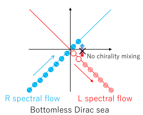
Figure 3: Spectral flows of right- and left-handed massless fermions in vacuum.

IV.2.2 Massive case

Next, we show that the paths of the spectral flows are changed for massive fermions (cf. Fig. 4), giving rise to a drastic change in the AWI. Also, we point out that chirality mixing by a finite mass term allows for a diabatic axial-charge creation.

The massive polarization function $\Pi_{\parallel}$ in Eq. (8) provides the AWI

$${\rm F.T.}\ \partial_{\mu}j_{A}^{\mu}=\frac{q_{f}^{2}}{2\pi^{2}}\tilde{\bm{E}}(q)\cdot{\bm{B}}\Big{[}\,1-I\big{(}\frac{q_{\parallel}^{2}}{4m^{2}}\big{)}\,\Big{]}e^{-\frac{|{\bm{q}}_{\perp}|^{2}}{2|q_{f}B|}}\,.$$ (22)

The unit term in the brackets is the same anomalous term as in the massless case (20). As explicitly identified in Appendix B, the other term is the matrix element of the pseudoscalar condensate $2im\langle\bar{\psi}\gamma^{5}\psi\rangle$, which automatically arises from computation of the massive fermion loop. In terms of the classical equation of motion, the origin of this term is easily identified with the explicit symmetry breaking by the fermion mass term in the Lagrangian. Nevertheless, the matrix element needs a one-loop diagram with insertion of the external photon field to take a nonzero value.

Notice that the anomalous term itself is independent of the mass scale since it originates from the ultraviolet regularization of the bottomless Dirac sea. In other words, the spectral flow from the bottom of the Dirac sea is always there. However, the magnitude of the axial-current generation, the manifestation of chiral anomaly in the infrared regime, depends on the relative magnitude to the pseudoscalar-condensate term that depends on the fermion mass.

One can discuss the adiabatic limit such that $q_{\parallel}^{2}/m^{2}\to 0$, where there is no invariant energy transfer from the electric field. This configuration corresponds to a constant electric field that is time-independent and homogeneous along the magnetic-field direction (see Appendix C for more explicit explanations). Note that the electric field can still have an inhomogeneity in the transverse plane when $|{\bm{q}}_{\perp}|$ is finite, giving the Gaussian factor. In the adiabatic limit, we have $I(0)=1$, so that the axial current is conserved, i.e.,

$$\lim_{q_{\parallel}^{2}/m^{2}\to 0}{\rm F.T.}\ \partial_{\mu}j_{A}^{\mu}=0\,.$$ (23)

This is a natural result because the weak electric field, perturbatively applied in Eq. (4b), cannot create massive on-shell fermions in an adiabatic process. Any finite value of mass corresponds to the “infinite mass” limit in the relative sense $q_{\parallel}^{2}/m^{2}\to 0$. This explains why the above result is independent of the fermion mass; Unity $(=m^{2}/m^{2})$ is the only one possible dimensionless combination when $q_{\parallel}^{2}\to 0$. The massless limit should be taken with a finite value of $q_{\parallel}^{2}$ as $q_{\parallel}^{2}/m^{2}\to\infty$, reproducing the massless limit (20) with $I(\infty)=0$.

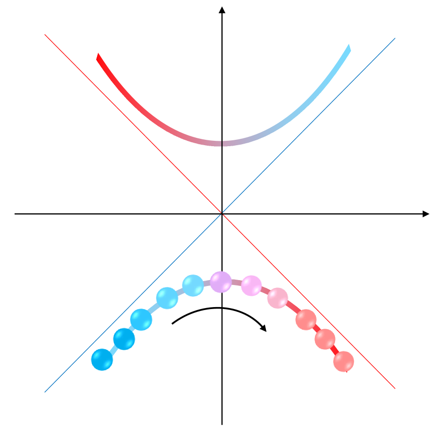
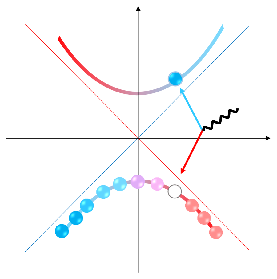
Figure 4: Adiabatic spectral flow of massive fermions in vacuum (left) and diabatic massive pair creation from a single photon in vacuum (right).

As clear in the above derivation (cf. Appendix B as well), the conservation of the axial current (23) simply means that a far-off-shell fermion loop vanishes when the fermion mass is much larger than any of external momenta, $q_{\parallel}^{2}/m^{2}\to 0$. Also, one can understand the conservation of the axial current in terms of the spectral flow along the parabolic curve in Fig. 4 (left). Since the positive- and negative-energy states are separated by the mass gap, the adiabatic spectral flow turns back to the bottom of the Dirac sea, creating no axial charge Ambjorn et al. (1983); Smilga (1992). This flow pattern is in a clear contrast to the massless case in Fig. 3. Below, we find that the medium contribution gives rise to an additional spectral flow.

In diabatic processes, a finite axial charge can be created with a finite energy transfer ($q_{\parallel}^{2}/m^{2}\not=0$) from non-constant electric fields. Remember that a fermion and antifermion pair can be created from a single photon in strong magnetic fields as discussed in Paper I. This process is possible only for massive fermions because the created pair has the same helicity along the magnetic field, requiring a chirality mixing at the vertex (see Appendix A for summary of the quantum numbers that specify the LLL fermions and antifermions). Once the process occurs, the created pair carries a net helicity, giving rise to a nonzero contribution to the AWI.

Figure 4 (right) exhibits a pair creation from a single photon. The chirality mixing by a finite fermion mass is expressed with a color gradient from red to blue. The mixing strength is maximum at $p_{z}=0$, and the fermion wave function approaches the chirality eigenstate in the large momentum regime $|p_{z}|/m\gg 1$. Therefore, when a created fermion is right-ish (left-ish) in chirality, an antiparticle can be left-ish (right-ish), creating a finite axial charge. The back-to-back kinematics is only allowed for massive fermions with this chirality mixing, and the diabatic pair creation is prohibited in the massless case. A similar prohibition mechanism is known as the “helicity suppression” in the leptonic decay of charged pions Donoghue et al. (1992); Zyla et al. (2020).

IV.3 Medium contributions

IV.3.1 Spectral flow in medium

Next, we consider the medium contributions. In contrast to the vacuum case, even a soft photon can perturb the systems when medium fermions are populated in the positive-energy states above the mass gap at finite temperature and/or density. In this case, the axial current will not be conserved if scatterings with single photons induce helicity flips. Including the medium contribution to $\Pi_{\parallel}$ obtained in Eq. (17), we find the AWI (21). Again, there is no correction to the anomalous term itself since the medium corrections do not change the (superficial) UV divergence. The medium part, proportional to the fermion mass, can be identified with the medium correction to the matrix element of the pseudoscalar condensate. Namely, including the medium correction, the pseudoscalar condensate in the LLL reads

$$2im\langle\bar{\psi}\gamma^{5}\psi\rangle = \frac{q_{f}^{2}}{2\pi^{2}}\tilde{\bm{E}}(q)\cdot{\bm{B}}\,e^{-\frac{|{\bm{q}}_{\perp}|^{2}}{2|q_{f}B|}}\left[w(\omega,q_{z})-1\right]\,,$$ (24)

with $w(\omega,q_{z})$ defined in Eq. (21). Those terms vanish in the massless limit, i.e., $w(\omega,q_{z})\to 1$, and the AWI (21) goes back to that in the massless limit (20).

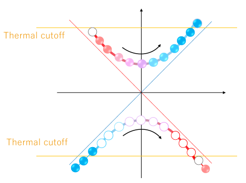
Figure 5: Spectral flows of massive fermions and antifermions (shown as holes) in medium.

We first discuss a drastic change in the spectral flow. In contrast to the vacuum case where the spectral flow of massive fermions does not generate an axial charge [cf. Eq. (23)], the spectral flows of medium particles can create axial charges as illustrated in Fig. 5. Notice that the Fermi-Dirac distribution function works as a finite cutoff to the loop momentum. This makes a big difference from the vacuum spectral flow beneath the bottomless Dirac sea (see Fig. 4 and the discussions there).

In the presence of the thermal cutoff, a state just above the thermal cutoff is filled after the spectral flow on the positive-energy branch and a previously occupied state just below the thermal cutoff is removed on the other wing of the parabolic dispersion curve (cf. Fig. 5). This process of course does not change the total particle number, but changes the helicity. What happens during this process is a momentum flip, and thus a helicity flip, across the “valley” of the parabolic dispersion curve. The same occurs in the positive-energy antiparticle branch, creating a net axial charge. This axial-charge creation is not anomalous in the sense that its origin is not related to the concept of infinity known with the “Hilbert hotel” Gamow (1988).

Indeed, the above axial-charge creation originates not from the anomalous term but from the mass-dependent pseudoscalar condensate term. Remarkably, the result will turn out to have the same form as the anomalous term in the adiabatic and high-temperature limits (or in the adiabatic and high-density limits). This is simply because the axial-charge imbalance appears near the thermal cutoff instead of the infrared regime, so that effects of the finite curvature along the dispersion curve is negligible in the high-temperature or high-density limit defined as $m/T,\ m/\mu\to 0$.

To verify the above statements, we examine the zero frequency and momentum limits. Though the results turn out to be independent of the ordering of the limits, one can consider the following two orderings:

$$\lim_{\omega/m\to 0}\lim_{q_{z}/m\to 0}{\rm F.T.}\ \partial_{\mu}j_{A}^{\mu} = \frac{q_{f}^{2}}{2\pi^{2}}\tilde{\bm{E}}(q)\cdot{\bm{B}}\,e^{-\frac{|{\bm{q}}_{\perp}|^{2}}{2|q_{f}B|}}\lim_{\omega/m\to 0}2m^{2}{\mathcal{P}}\int_{-\infty}^{\infty}\frac{dp_{z}}{\epsilon_{p}}\frac{n_{+}(\epsilon_{p})+n_{-}(\epsilon_{p})}{(2\epsilon_{p})^{2}-\omega^{2}}\,,$$

$$\lim_{q_{z}/m\to 0}\lim_{\omega/m\to 0}{\rm F.T.}\ \partial_{\mu}j_{A}^{\mu} = \frac{q_{f}^{2}}{2\pi^{2}}\tilde{\bm{E}}(q)\cdot{\bm{B}}\,e^{-\frac{|{\bm{q}}_{\perp}|^{2}}{2|q_{f}B|}}\lim_{q_{z}/m\to 0}\left(-\frac{m^{2}}{q_{z}}\right){\mathcal{P}}\int_{-\infty}^{\infty}\frac{dp_{z}}{\epsilon_{p}}\frac{n_{+}(\epsilon_{p})+n_{-}(\epsilon_{p})}{p_{z}-\frac{1}{2}q_{z}}\,,$$

where ${\mathcal{P}}$ denotes the principal value. The vacuum contribution vanishes in these limits according to Eq. (13). We have encountered the same integrals in Sec. IV of Paper I when computing the photon masses, where the orderings do matter. The distribution functions can be simply replaced by the upper and lower boundaries of the integrals in the high-$T$ or high-$\mu$ limit, leading to simple results

$$\lim_{\Lambda/m\to\infty}\lim_{\omega/m\to 0}2m^{2}{\mathcal{P}}\int_{-\Lambda}^{\Lambda}\frac{dp_{z}}{\epsilon_{p}}\frac{1}{(2\epsilon_{p})^{2}-\omega^{2}}=1\,,$$ (26a)

$$\lim_{\Lambda/m\to\infty}\lim_{q_{z}/m\to 0}\left(-\frac{m^{2}}{q_{z}}\right){\mathcal{P}}\int_{-\Lambda}^{\Lambda}\frac{dp_{z}}{\epsilon_{p}}\frac{1}{p_{z}-\frac{1}{2}q_{z}}=1\,,$$ (26b)

where $\Lambda=T$ or $\mu$. Note that a hierarchy $T/\mu\gg 1$ ($T/\mu\ll 1$) needs to be satisfied for the above replacement, in addition to the high-temperature limit $m/T\to 0$ (high-density limit $m/\mu\to 0$). Plugging the above integrals into Eq. (25), one finds the AWI in the adiabatic and high-temperature (or high-density) limits

$$\lim_{\omega/m\to 0}\lim_{q_{z}/m\to 0}{\rm F.T.}\ \partial_{\mu}j_{A}^{\mu}=\lim_{q_{z}/m\to 0}\lim_{\omega/m\to 0}{\rm F.T.}\ \partial_{\mu}j_{A}^{\mu} = \frac{q_{f}^{2}}{2\pi^{2}}\tilde{\bm{E}}(q_{\perp})\cdot{\bm{B}}\,e^{-\frac{|{\bm{q}}_{\perp}|^{2}}{2|q_{f}B|}}\,.$$ (27)

Notice that the medium contribution to the pseudoscalar condensate results in the same form as the anomalous term. This mechanism is rather similar to the “chiral anomaly” in lattice models; The approximate linear dispersion relations are connected with each other as segments of the periodic dispersion relations, forming a valley similar to Fig. 5. In short, we have explicitly seen that the axial charge is generated by the spectral flow of thermally populated fermions even when the spectral flow beneath the Dirac sea cannot contribute at all.

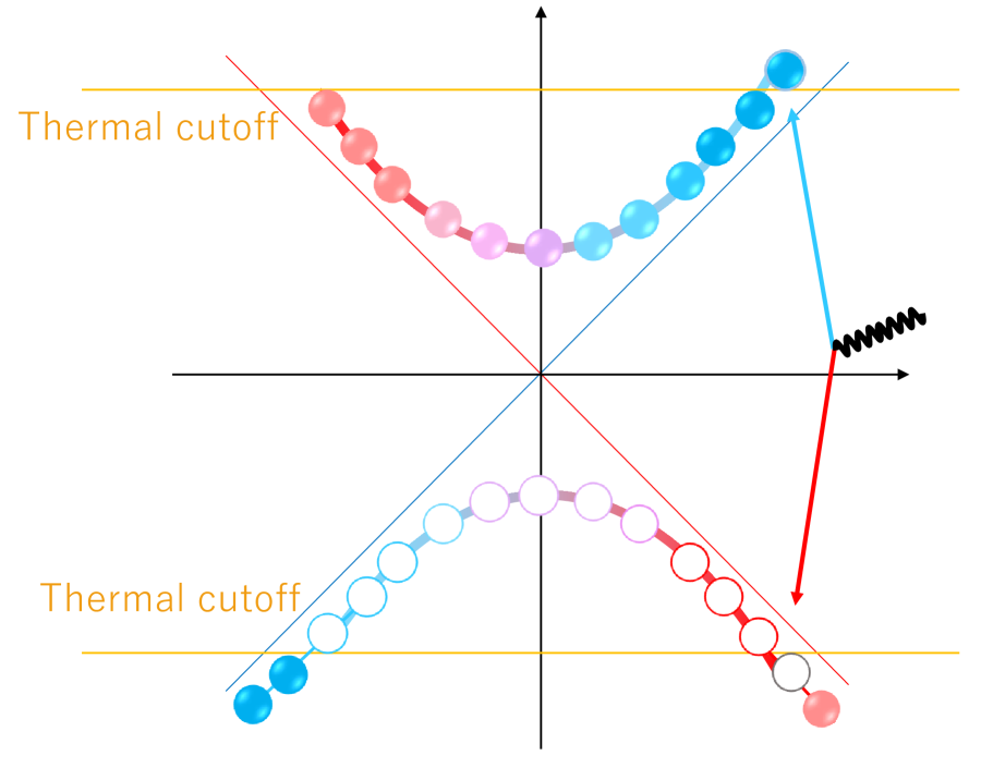
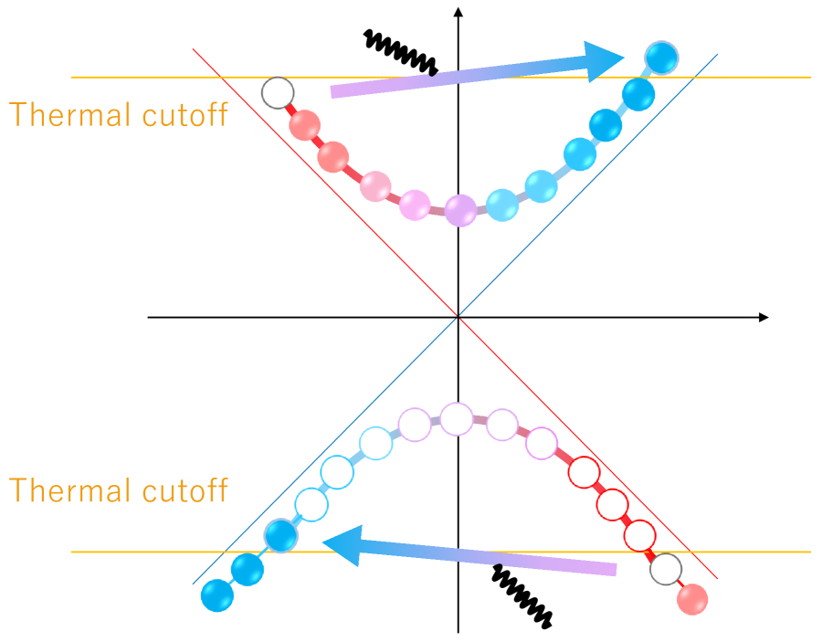
Figure 6: Axial-charge creation from the pair creation (left) and the Landau damping (right).

IV.3.2 Diabatic processes

When the electric field has a finite frequency $\omega$, the pair creation and the Landau damping can contribute to the integral in Eq. (24). The electric field can be both external one and of a dynamical photon as long as its magnitude is perturbatively weak. According to the optical theorem, nonzero rates of those reactions are directly captured by the imaginary part of the polarization tensor that gives a real part of the induced axial current just like electric currents are expressed by imaginary parts of the retarded correlators according to the Kubo formula. The real part of the polarization tensor also exhibits peak structures originating from those reactions (see Sec. III. B in Paper I); The real and imaginary parts are related to each other via the dispersion integral, and are two sides of the same coin.

Kinematics in the relevant processes are shown in Fig. 6. We have discussed the contribution from the pair creation in Sec. IV.2.2 in vacuum case. The medium correction should suppress the pair creation due to the Pauli-blocking effect in the final state when the photon energy is smaller than the temperature and/or density scale. On the other hand, the Landau damping is a pure medium effect in which a medium fermion is scattered off an off-shell photon. The scatterings from one side to the other side of the parabolic dispersion relation is accompanied by a helicity flip. We have inspected those reactions in Paper I by performing the same integral as that in Eq. (24).

To understand basic behaviors of $w(\omega,q_{z})$ defined in Eq. (21), we consider the homogeneous limit ($q_{z}\to 0$)

$$\lim_{q_{z}/m\to 0}w(\omega,q_{z})=1-I\big{(}\frac{\omega^{2}}{4m^{2}}\big{)}+2m^{2}{\mathcal{P}}\int_{-\infty}^{\infty}\frac{dp_{z}}{\epsilon_{p}}\frac{n_{+}(\epsilon_{p})+n_{-}(\epsilon_{p})}{(2\epsilon_{p})^{2}-\omega^{2}}\,,$$ (28)

where the electric field may still have a transverse inhomogeneity $|{\bm{q}}_{\perp}|\not=0$. The left panel in Fig. 7 shows the real and imaginary parts of $w(\omega)$ with blue and red lines, respectively. The colored dashed lines show the vacuum contributions. The adiabatic limit corresponds to the interception at $\omega=0$ that vanishes in vacuum as discussed above, but takes finite values in medium. We compare the low- and high-temperature cases with $T/m=0.5$ (darker color) and $T/m=1.5$ (lighter color) at zero density $\mu/m=0$. As we increase temperature, the real part approaches the constant value $w(\omega)=1$ in the massless limit. The imaginary part above the threshold, on the right of the dashed vertical line, gives the contribution from the pair creation. The imaginary part diverges as $\omega$ approaches the threshold from above. Correspondingly, the real part also diverges as $\omega$ approaches the threshold from below. Those behaviors are typical threshold behaviors in (1+1) dimensions and manifest themselves here because of the effective dimensional reduction in the strong magnetic fields. The sign of the real part depends on $\omega$, which is due to a phase lag in response to time-dependent electric fields.

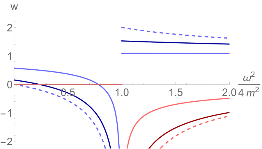
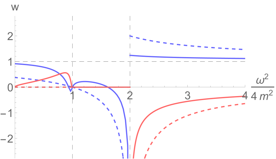
Figure 7: $w(\omega,q_{z})$ for the AWI at $q_{z}=0$ in the homogeneous limit [left] and at $q_{z}/(2m)=1$ [right]. The blue and red lines show the real and imaginary parts, respectively. We take temperature scales $T/m=0.5$ (the darker colors) and $T/m=1.5$ (the lighter colors) at zero density $(\mu=0)$, while the vacuum contribution is shown with dashed lines.

In the right panel of Fig. 7, we show the AWI at a finite value of momentum $q_{z}/(2m)=1$. We take $T/m=1.5$ and $\mu/m=0$ as in the left panel. When $\omega$ is small, there is a spatial region $\omega^{2}-q_{z}^{2}<0$ on the leftmost side of the dashed vertical lines. In this region, the imaginary part, shown with the red line, solely stems from the Landau damping. In the adiabatic or stationary limit ($\omega\to 0$), the imaginary part, however, vanishes for any value of $q_{z}$ since imaginary parts of retarded correlators are odd functions of $\omega$ on the general ground. There appears a negative peak structure in the real part corresponding to the peak structure in the imaginary part. Qualitative behaviors in the other regions are common to the left panel at $q_{z}=0$. Both the real and imaginary parts go through the point $w(\omega=q_{z},q_{z})=0$ where $q_{\parallel}^{2}=0$.

Finally, we show the AWI at zero temperature and a finite chemical potential $\mu/m=2$ in Fig. 8. We take $q_{z}/(2m)=1$ as in Fig. 7. Remarkably, the diverging threshold behavior at $q_{\parallel}^{2}=4m^{2}$ shifts to a higher energy. This is due to the Pauli-blocking effect; Since the positive-energy states are occupied up to the sharp Fermi surface, the pair creation can only occur in vacant states above the Fermi surface, requiring a larger energy of the order of the chemical potential. The singular behaviors at the threshold is now logarithmic and the threshold position splits into this one and a higher one that is outside the plot region (see Paper I for more discussions). The Landau damping also gives rise to step singularities in the imaginary part since it brings one occupied state below the sharp Fermi surface to a vacant state above the Fermi surface. Finite-temperature effects make vacancy below the Fermi surface, so that the threshold position goes back to $q_{\parallel}^{2}=4m^{2}$ at finite temperature.

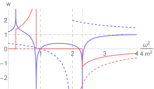
Figure 8: $w(\omega,q_{z})$ for the AWI at zero temperature and a finite chemical potential $\mu/m=2$. We take $q_{z}/(2m)=1$ as in Fig. 7.

V Summary and discussions

In this paper, we investigated the AWI in the LLL approximation that is composed of the anomalous and pseudoscalar-condensate terms. The AWI is saturated by the anomalous term in the massless case irrespective of the presence or absence of the medium. The polarization tensor, the central quantity in this series of papers, describes the medium corrections to the pseudoscalar condensate which, therefore, should be proportional to the fermion mass. We showed how the AWI as a whole behaves when we vary temperature and/or density as well as the fermion mass and the external photon momentum. We classified the mechanisms of the axial-charge generation into the adiabatic and diabatic processes.

For the adiabatic processes, we further classified the patterns of the spectral flows putting an emphasis on two simple points, that is, the shape of dispersion relation and whether or not the states on the dispersion relation are occupied. The spectral flows take the paths along the dispersion relations, and thus there is a qualitative difference between the massless and massive cases. A nonzero axial charge could only stem from the spectral flow of the positive-energy states in the massive case since the anomalous term is offset by the vacuum part of the pseudoscalar condensate in the adiabatic limit. Therefore, a nonzero axial charge is generated by the helicity flip on the medium particles and does not contain a contribution from the anomalous term; The AWI is dominated by the medium contribution. It is remarkable that the medium contribution, nevertheless, agrees with the anomalous term in the high-temperature or high-density limit as compared to the fermion mass, where the curvature of the parabolic dispersion relation is negligible. We showed those limiting behaviors in an analytic way and would like to add that there are possible contributions from the higher Landau levels in such limits, which needs to be investigated in the future works.

We also investigated the diabatic contributions to the axial-charge generation which can be finite only for massive fermions. The relevant physical processes are the pair creation from a single photon and the Landau damping. Those processes are not anomalous in the sense that they are nothing to do with the ultraviolet divergence. Thus, there are possible higher-order radiative corrections. Such corrections in QED may be small in many of relevant applications in vacuum. However, when scatterings with medium particles happen so frequently in high-energy-density states, such corrections can be significant even in weak-coupling theories. In addition, there are possible contributions from the higher Landau levels. Remember that the AWIs from the LLL approximation and the triangle diagrams only agree with each other in the homogeneous limit $|{\bm{q}}_{\perp}|^{2}/|q_{f}B|\to 0$ as explicitly shown in Appendix C. The discrepancy needs to be compensated by contributions from the higher Landau levels, and can be significant when the higher Landau levels are excited at the temperature and/or density scale comparable to the magnetic-field strength. Such environments can be realized in relativistic heavy-ion collisions, neutron star, and the early universe depending on detailed situations. We leave those points and applications as future works.

Studying the axial-charge dynamics provides implications for various systems. The amount of the created axial charge determines the magnitude of the CME currents induced in relativistic heavy-ion collisions Kharzeev et al. (2016); Skokov et al. (2017); Hattori and Huang (2017); Abdallah et al. (2022) and the Weyl and Dirac semimetals Burkov (2015); Gorbar et al. (2018); Armitage et al. (2018). The axial-charge dynamics even plays a crucial role when the magnetic fields are dynamical and are subject to the chiral plasma instability that has been discussed as a possible origin of the strong magnetic fields in the early universe and neutron stars/magnetars Turner and Widrow (1988); Carroll et al. (1990); Garretson et al. (1992); Joyce and Shaposhnikov (1997); Giovannini (2004); Laine (2005); Akamatsu and Yamamoto (2013, 2014). The time evolution of the axial-charge density should be tracked consistently coupled to the amplification of the magnetic fields. In addition to those CME-induced phenomena, one can study the axial-charge dynamics revealing itself in the optical activities. Such directions have been pursued with the Weyl and Dirac semimetals Zhou et al. (2015); Behrends et al. (2016); Tabert et al. (2016); Yang et al. (2018); Sonowal et al. (2019); Song et al. (2016); Rinkel et al. (2017); Hui et al. (2019); Yuan et al. (2020); Almutairi et al. (2020); Gao and Zhang (2021); Singh and Carbotte (2021); Long et al. (2018); Tse and MacDonald (2010); Liang et al. (2021); Kargarian et al. (2015); Tokman et al. (2020). It is interesting to investigate possible optical signals form the quark-gluon plasma and from the outer space as well.

There is another implication for the production of axion or any hypothetical pseudoscalar particles via the Primakoff effect Sikivie (1983, 1985); Raffelt (1986); Raffelt and Stodolsky (1988); Raffelt (1990). This mechanism can be understood as a mixing process between a single photon and the single pseudoscalar particle in strong magnetic fields of stars or galaxies. The similar idea leads to the light-shining-through-wall experiment in laboratories (see, e.g., Refs. Gies (2009); Redondo and Ringwald (2011) for reviews). The two-point function between the axial and vector currents studied in this paper determines the mixing strength with the inclusion of the screening effect in medium. The screening effect can be important in stars and galaxies, giving rise to the nontrivial peak structures in the photon-energy and -momentum dependences shown in this paper. This deserves further studies in fundamental physics.

Acknowledgments.— KH thanks Patrick Copinger, Kenji Fukushima, Yoshimasa Hidaka, Xu-Guang Huang, Hidetoshi Taya, and Di-Lun Yang for discussions. This work is supported in part by JSPS KAKENHI under grant Nos. 20K03948 and 22H02316.

Appendix A Massless fermions and antifermions in the LLL

We summarize the quantum numbers characterizing the LLL fermions and antifermions to clarify somewhat confusing terminologies. For clarity, we here assign the following terminologies.

“Chirality” is an eigenvalue of $\gamma^{5}$ that specifies the handedness of the spinor $\psi_{R/L}$, i.e., $\gamma^{5}\psi_{R/L}=\pm\psi_{R/L}$ with the upper/lower signs for $R/L$. “Axial charge” is the difference between the number densities $j_{A}^{0}=n_{R}-n_{L}$ created by the spinors $\psi_{R/L}$. Since antiparticles are counted in the net number densities with negative signs, they contribute to the axial charge with opposite signs to the particle contributions. Those correspondences are summarized in Table 1.

“Helicity” is defined by the relative direction between spin and momentum as $h=S_{z}p_{z}/|p^{0}|$ with the spin operator $S_{z}=i\gamma^{1}\gamma^{2}/2$. The correspondence to chirality is made clear if one refers to the Dirac operator. The fermion spinor $\psi_{\rm LLL}$ for the LLL should satisfy the following Dirac equation (see Paper I)

$$(p^{0}-s_{f}p_{z}\gamma^{5})\psi_{\rm LLL}=0\,,$$ (29)

where we used the fact that the LLL spinor is an eigenfunction of the spin operator $2S_{z}\psi_{\rm LLL}=(i\gamma^{1}\gamma^{2})\psi_{\rm LLL}=s_{f}\psi_{\rm LLL}$. Therefore, one finds that

$$h\,\psi_{\rm LLL}=\frac{1}{2}{\rm sgn}(p^{0})\gamma^{5}\psi_{\rm LLL}\,,$$ (30)

where $(\gamma^{5})^{2}=1$. The relative sign between the chirality and the helicity depends on the sign of the energy. Therefore, $\psi_{\rm LLL}^{R}$ ($\psi_{\rm LLL}^{L}$) contains the right-handed helicity particles and left-handed helicity antiparticles (the left-handed helicity particles and right-handed helicity antiparticles). The particles and (positive-energy) antiparticles should have opposite helicities because they move in the same directions but have opposite spin directions due to the Zeeman effect. Helicity is independent of the sign function $s_{f}$, because both the spin and momentum directions depend on $s_{f}$.

Massive fermions are none of those eigenstates, and are the mixed states of them as shown in Figs. 4 and 5 with the color gradient. Some scattering processes require such chirality mixing to occur with finite amplitudes.

Table 1: Quantum numbers that specify the massless LLL fermions and antifermions. The upper and lower signs are for the right- and left-handed chirality sectors, respectively.

	Spin $(S_{z})$	Chirality $(\gamma^{5})$	Axial charge $(j_{A}^{0})$	Momentum $(p_{z})$	Helicity $(S_{z}p_{z}/|p_{z}|)$
Particles	$+s_{f}\frac{1}{2}$	$\pm 1$	$\pm 1$	$\pm s_{f}$	$\pm\frac{1}{2}$
Antiparticles	$-s_{f}\frac{1}{2}$	$\pm 1$	$\mp 1$	$\pm s_{f}$	$\mp\frac{1}{2}$

Appendix B Chiral anomaly diagram with massive LLL fermions

In this Appendix, we directly compute the anomaly diagram with massive fermions in the LLL and demonstrate that it splits into the anomalous term and the matrix element of the pseudoscalar condensate. One can also explicitly confirm that the anomalous term is independent of the fermion mass, while the latter is proportional to the fermion mass required by the chirality mixing in the pseudoscalar fermion bilinear.

We examine the two-point function composed of the LLL fermion loop:

$$\int d^{4}x\,e^{-iqx}\langle k|\partial_{\mu}j_{A}^{\mu}(x)|0\rangle=\rho_{B}e^{-\frac{|{\bm{q}}_{\perp}|^{2}}{2|q_{f}B|}}(2\pi)^{2}\delta^{(2)}(k_{\parallel}-q_{\parallel})iq_{\mu}\Pi_{1+1(A)}^{\mu\nu}(q_{\parallel})\epsilon^{\ast}_{\nu}(q)\,.$$ (31)

The Landau degeneracy factor and the Gaussian come from the transverse-momentum integral as in the computation of the vector-current correlator (cf. Paper I). The residual (1+1)-dimensional longitudinal part is given as

$$iq_{\mu}\Pi_{1+1(A)}^{\mu\nu}(q_{\parallel})=(-1)(-iq_{f})\int\!\!\frac{d^{2}p_{\parallel}}{(2\pi)^{2}}\frac{{\rm tr}[\,\not{q}_{\parallel}\gamma^{5}i(\not{p}_{\parallel}+m){\mathcal{P}}_{+}\gamma_{\parallel}^{\nu}i(\,(\not{p}_{\parallel}+\not{q}_{\parallel})+m\,){\mathcal{P}}_{+}\,]}{(p_{\parallel}^{2}-m^{2})(\,(p_{\parallel}+q_{\parallel})^{2}-m^{2}\,)}\,.$$ (32)

The two-dimensional integral has a (superficial) logarithmic divergence, and we use the dimensional regularization.

It is important to make sure the properties of the $\gamma^{5}$ to apply the dimensional regularization. The $\gamma^{5}$ is extended in such a way that $\{\gamma^{5},\gamma^{\mu}\}=0$ for $\mu=0,1,2,3$ and $[\gamma^{5},\gamma^{\mu}]=0$ for the other extra components. The extra components in the momentum is denoted with tilde like $\tilde{\ell}^{\mu}$, which corersponds to $\ell_{\perp}^{\mu}$ in the notations of Ref. Peskin and Schroeder (1995). The external momenta $q^{\mu},k^{\mu}$ have vanishing components in the extra dimensions, $\tilde{q}^{\mu}=\tilde{k}^{\mu}=0$. The extra components of $\gamma^{\mu}$ commute with $\gamma^{5}$, i.e., $[\tilde{\not{\ell}},\gamma^{5}]=0$. Then, one can show an identity

$$\not{q}_{\parallel}\gamma^{5}=\gamma^{5}(\not{p}_{\parallel}-m)+(\not{q}_{\parallel}+\not{p}_{\parallel}-m)\gamma^{5}+2(m-\tilde{\not{p}}_{\parallel})\gamma^{5}\,.$$ (33)

Plugging the identity (33) into the (1+1)-dimensional part, we have

$$iq_{\mu}\Pi_{1+1(A)}^{\mu\nu}(q_{\parallel})\epsilon^{\ast}_{\nu}(q) = q_{f}\epsilon^{\ast}_{\nu}(q)\int\!\!\frac{d^{d}p_{\parallel}}{(2\pi)^{d}}\left[\,\frac{{\rm tr}[\,\gamma^{5}{\mathcal{P}}_{+}\gamma_{\parallel}^{\nu}(\,(\not{p}_{\parallel}+\not{q}_{\parallel})+m\,)\,]}{(p_{\parallel}+q_{\parallel})^{2}-m^{2}}+\frac{{\rm tr}[\,\gamma^{5}{\mathcal{P}}_{+}(\not{p}_{\parallel}+m)\gamma_{\parallel}^{\nu}\,]}{p_{\parallel}^{2}-m^{2}}\,\right]$$ (34)

$$-2q_{f}\epsilon^{\ast}_{\nu}(q)\int\!\!\frac{d^{d}p_{\parallel}}{(2\pi)^{d}}\frac{{\rm tr}[\,\tilde{\not{p}}_{\parallel}\gamma^{5}(\not{p}_{\parallel}+m){\mathcal{P}}_{+}\gamma_{\parallel}^{\nu}(\,(\not{p}_{\parallel}+\not{q}_{\parallel})+m\,){\mathcal{P}}_{+}\,]}{(p_{\parallel}^{2}-m^{2})(\,(p_{\parallel}+q_{\parallel})^{2}-m^{2}\,)}$$

$$+2im\langle\bar{\psi}\gamma^{5}\psi\rangle\,.$$

Each of the two terms in the square brackets vanishes because the integral and trace vanish if one picks up the momentum and mass factors in the trace, respectively. The last term is identified with the matrix element of the pseudoscalar condensate

$$\langle\bar{\psi}\gamma^{5}\psi\rangle=(-1)[-iq_{f}\epsilon^{\ast}_{\nu}(q)]\int\!\!\frac{d^{2}p_{\parallel}}{(2\pi)^{2}}\frac{{\rm tr}[\,\gamma^{5}i(\not{p}_{\parallel}+m){\mathcal{P}}_{+}\gamma^{\nu}_{\parallel}i(\,(\not{p}_{\parallel}+\not{q}_{\parallel})+m\,){\mathcal{P}}_{+}\,]}{(p_{\parallel}^{2}-m^{2})(\,(p_{\parallel}+q_{\parallel})^{2}-m^{2}\,)}\,.$$ (35)

This is the leading nonvanishing contribution from the diagram with one-insertion of the external photon leg. The remaining term in Eq. (34) will result in the anomalous term.

We shall first examine the anomalous term. Introducing the Feynman parameter, one can make a complete square in the denominator $x(p_{\parallel}^{2}-m^{2})+(1-x)(\,(p_{\parallel}+q_{\parallel})^{2}-m^{2})=\{p_{\parallel}+(1-x)q_{\parallel}\}^{2}-\Delta_{\parallel}$ with $\Delta_{\parallel}=m^{2}-x(1-x)q_{\parallel}^{2}$. We then shift the integral variable as $p_{\parallel}^{\prime}=p_{\parallel}+(1-x)q_{\parallel}$ that is allowed after the divergence is regularized. To have a nonvanishing trace, one should pick up $\gamma^{1}\gamma^{2}$ in ${\mathcal{P}}_{+}$. To have a nonvanishing integral for the extra dimension, one needs to pick up one $\not{p}_{\parallel}$ from the propagator. Then, one needs to take the photon momentum $\not{q}_{\parallel}$ in the other fermion propagator to make both the trace and integral nonvanishing. Therefore, assuming the presence of the integral, we have

$${\rm tr}[\,\tilde{\not{p}}_{\parallel}\gamma^{5}(\not{p}_{\parallel}-(1-x)\not{q}_{\parallel}+m){\mathcal{P}}_{+}\gamma_{\parallel}^{\nu}(\,(\not{p}_{\parallel}+x\not{q}_{\parallel})+m\,){\mathcal{P}}_{+}\,]=-2s_{f}q_{\parallel\mu}\epsilon^{\mu\nu 12}\tilde{p}_{\parallel}^{2}\,.$$ (36)

The mass dependence as well as the Feynman parameter go away from the trace. Then, the momentum integral reads

$$\int\!\!\frac{d^{d}p_{\parallel}}{(2\pi)^{d}}\frac{\tilde{p}_{\parallel}^{2}}{(p_{\parallel}^{2}-\Delta_{\parallel})^{2}}=\frac{d-2}{d}\times\frac{(-1)i}{(4\pi)^{d/2}}\frac{d}{2}\frac{\Gamma(-\frac{d-2}{2})}{\Gamma(2)}\Delta_{\parallel}^{\frac{d-2}{2}}=\frac{i}{4\pi}\,,$$ (37)

where we used $(d-2)\Gamma(-\frac{d-2}{2})=-2+{\mathcal{O}}(d-2)$. The integral is finite because of the overall dimensional factor $(d-2)$. All the subleading terms vanish thanks to the same overall factor, and thus the integral is given by the above universal form. Then, we obtain the (1+1) dimensional AWI

$$iq_{\mu}\Pi_{1+1(A)}^{\mu\nu}(q_{\parallel})\epsilon^{\ast}_{\nu}(k)=-\frac{q_{f}}{\pi}\langle k|\tilde{E}_{\parallel}|0\rangle+2im\langle\bar{\psi}\gamma^{5}\psi\rangle\,,$$ (38)

where the momentum conservation in Eq. (31) is understood (with the delta function suppressed). As in Eq. (4), the Fourier spectrum of the electric field is defined as $\tilde{E}_{\parallel}(q)=-i\epsilon^{\mu\nu}_{\parallel}q_{\mu}A_{\nu}$ with $\epsilon^{\mu\nu}_{\parallel}=\epsilon^{\mu\nu 12}$.

Next, we compute the pseudoscalar condensate

$$\langle\bar{\psi}\gamma^{5}\psi\rangle=\frac{s_{f}q_{f}}{2}\epsilon^{\ast}_{\nu}(q)\int_{0}^{1}dx\int\!\!\frac{d^{2}p_{\parallel}}{(2\pi)^{2}}\frac{{\rm tr}[\,\gamma^{5}\gamma^{1}\gamma^{2}(\not{p}_{\parallel}-(1-x)\not{q}_{\parallel}+m)\gamma^{\nu}_{\parallel}(\,(\not{p}_{\parallel}+x\not{q}_{\parallel})+m\,)\,]}{(p_{\parallel}-\Delta_{\parallel})^{2}}\,.$$

The integral is finite. One needs to take $\gamma^{1}\gamma^{2}$ in ${\mathcal{P}}_{+}$ because four gamma matrices are required for a nonzero result of the trace with one $\gamma^{5}$. For the same reason, one needs to pick up one mass term, reflecting the fact that the chirality needs to be flipped. Then, there is no room for $\not{p}_{\parallel}$ to be included so that the integral becomes nonvanishing. Therefore, the trace under the momentum integral reads

$${\rm tr}[\,\gamma^{5}\gamma^{1}\gamma^{2}(\not{p}_{\parallel}-(1-x)\not{q}_{\parallel}+m)\gamma^{\nu}_{\parallel}(\,(\not{p}_{\parallel}+x\not{q}_{\parallel})+m\,)\,]=m{\rm tr}[\,\gamma^{5}\gamma^{1}\gamma^{2}\gamma^{\nu}_{\parallel}\not{q}_{\parallel}\,]\,.$$ (40)

The matrix element of the pseudoscalar condensate is proportional to the fermion mass because the pseudoscalar fermion bilinear mixes the chirality, requiring that the mass term induce chirality mixing odd times on the loop diagram.

The $x$-dependent terms cancel away. The remaining elementary integrals are performed as

$$\int_{0}^{1}dx\int\!\!\frac{d^{2}p_{\parallel}}{(2\pi)^{2}}\frac{1}{(p_{\parallel}-\Delta_{\parallel})^{2}}=\frac{i}{4\pi}\int_{0}^{1}\frac{dx}{m^{2}-x(1-x)q_{\parallel}^{2}}=\frac{i}{4\pi m^{2}}I\left(\frac{q_{\parallel}^{2}}{4m^{2}}\right)\,,$$ (41)

yielding the $I$ function defined in Eq. (12). Thus, the matrix element of the pseudoscalar condensate is given as

$$2im\langle\bar{\psi}\gamma^{5}\psi\rangle=\frac{s_{f}q_{f}}{\pi}\tilde{E}_{\parallel}(q)I\Big{(}\frac{q_{\parallel}^{2}}{4m^{2}}\Big{)}\,.$$ (42)

Combining the anomalous term and pseudoscalar condensate in Eq. (38) reproduces the AWI (22) obtained from the polarization function $\Pi_{\parallel}$ in Eq. (8). Explicitly, we have obtained

$${\rm F.T.}\ \partial_{\mu}j_{A}^{\mu}=\frac{q_{f}^{2}}{2\pi^{2}}\tilde{\bm{E}}(q)\cdot{\bm{B}}\Big{[}\,1-I\Big{(}\frac{q_{\parallel}^{2}}{4m^{2}}\Big{)}\,\Big{]}e^{-\frac{|{\bm{q}}_{\perp}|^{2}}{2|q_{f}B|}}\,.$$ (43)

We emphasize that both the mass-independent anomalous term and the mass-dependent pseudoscalar condensate originate from the same diagram composed of the massive fermion loop. The massive fermion loop vanishes as a whole in the large-mass limit, $\lim_{x\to 0}I(x)=1$. This clearly explains the vanishing behavior observed below Eq. (22).

Appendix C Relation to the triangle diagrams

Finally, we would like to establish an explicit connection between the AWI (22) from the LLL approximation and the perturbative one from the familiar triangle diagrams (cf. Fig 1). The triangle diagrams are perturbatively computed in the linear orders in the electric- and magnetic-field strengths and contains the ABJ anomaly in (3+1) dimensions Bell and Jackiw (1969); Adler (1969). On the other hand, the LLL approximation only appears after the resummation of one-loop diagrams to all orders with respect to insertion of the external legs for the constant magnetic field; The all-order resummation gives the fermion propagator the pole positions at the Landau levels. Thus, the triangle diagrams are contained in the resummed series but does not exactly correspond to the one-loop polarization tensor in the LLL. It is a non-trivial issue how the LLL approximation and the triangle diagrams are connected with each other, though the ABJ anomaly in (3+1) dimensions is often explained as a product of the Landau degeneracy factor and the (1+1) dimensional anomaly in the LLL Nielsen and Ninomiya (1983). In this appendix, we explicitly discuss their connection including the pseudoscalar-condensate term, focusing on zero temperature and density case.

Computing the massive triangle diagrams in Fig. 1, one finds the AWI Adler (1969)

$${\rm F.T.}\ \langle p,k|\partial_{\mu}j^{\mu}_{A}|0\rangle = \frac{q_{f}^{2}}{2\pi^{2}}\cdot\frac{1}{2}[\tilde{\bm{E}}(k)\cdot\tilde{\bm{B}}(p)+\tilde{\bm{B}}(k)\cdot\tilde{\bm{E}}(p)]$$

$$\times\Big{[}\,1+\int_{0}^{1}dx\int_{0}^{1-x}dy\frac{2m^{2}}{x(1-x)k^{2}+y(1-y)p^{2}+2xy\,p\cdot k-m^{2}}\,\Big{]}\,,$$

where $p$ and $k$ are the two photon momenta and are related to that of the axial current as $q^{\mu}=p^{\mu}+k^{\mu}$ according to the momentum conservation. The first and second terms in the brackets are the anomalous term and the matrix element of the pseudoscalar condensate, respectively. The tilde on the field strengths stands for the Fourier spectrum throughout the paper.

We show that the AWIs in Eqs. (22) and (C) exactly agree with each other in a certain limit. This agreement occurs in the limit where one of the photon momentum is zero while the other is finite. We shall take $p^{\mu}\to 0$, and then $q^{\mu}=k^{\mu}$ led by the momentum conservation. Then, the AWI (C) reads

$$\left.{\rm F.T.}\ \langle p,k|\partial_{\mu}j^{\mu}_{A}|0\rangle\right|_{p=0} = \frac{q_{f}^{2}}{2\pi^{2}}\cdot\frac{1}{2}[\tilde{\bm{E}}(q)\cdot\tilde{\bm{B}}(0)+\tilde{\bm{B}}(q)\cdot\tilde{\bm{E}}(0)]\Big{[}\,1-I\Big{(}\frac{q^{2}}{4m^{2}}\Big{)}\,\Big{]}\,.$$ (45)

Remarkably, the integral in Eq. (C) has reduced to the $I$ function (12) involved in the LLL approximation. One can show this reduction as follows. We have

$$\int_{0}^{1}dx\int_{0}^{1-x}dy\frac{2m^{2}}{x(1-x)k^{2}-m^{2}}=\int_{0}^{1}dx\frac{2m^{2}(1-x)}{x(1-x)k^{2}-m^{2}}\,,$$ (46)

and notice the identical transformations

$$\int_{0}^{1}dx\frac{2m^{2}(1-x)}{x(1-x)k^{2}-m^{2}} = \int_{0}^{1}dx\frac{2m^{2}x}{(1-x)xk^{2}-m^{2}}=\frac{1}{2}\int_{0}^{1}dx\frac{2m^{2}}{x(1-x)k^{2}-m^{2}}$$ (47)

$$= -I(k^{2}/4m^{2})\,.$$

The sum of the first two expressions results in the third expression that is nothing but the $I$ function. When one sends the other momentum $k^{\mu}$ to zero and maintains a finite value of $p^{\mu}$, the integral reduces to the $I$ function in the same manner. We consider the case of $\tilde{\bm{E}}(0)=0$. Summing the two contributions from $\tilde{\bm{B}}(p=0)$ and $\tilde{\bm{B}}(k=0)$ in Eq. (C), we obtain

$${\rm F.T.}\ \langle q|\partial_{\mu}j^{\mu}_{A}|0\rangle = \frac{q_{f}^{2}}{2\pi^{2}}\tilde{\bm{E}}(q)\cdot\tilde{\bm{B}}(0)\Big{[}\,1-I\Big{(}\frac{q^{2}}{4m^{2}}\Big{)}\,\Big{]}\,.$$ (48)

Therefore, the AWI (22) in the LLL agrees with Eq. (48) when one further assumes a homogeneity, i.e., $|{\bm{q}}_{\perp}|=0$, in the plane transverse to the magnetic field. In this limit, the Gaussian factor goes away in Eq. (22) and the squared momentum $q^{2}$ reduces to $q_{\parallel}^{2}$.

Now, we show that the vanishing momentum limit corresponds to a constant electromagnetic field (though the gauge field itself depends on the spacetime coordinate). Remember that the LLL contribution is computed in the homogeneous limit. For simplicity, we may consider a parallel electromagnetic field in the third spatial direction. Such a parallel field can be described by a linear gauge configuration

$$A^{\mu}(x)=(-c_{0}zE_{0}({\bm{x}}_{\perp}),-d_{1}yB_{0}(t,z),d_{2}xB_{0}(t,z),-c_{3}tE_{0}({\bm{x}}_{\perp}))\,,$$ (49)

with constants such that $c_{0}+c_{3}=1$ and $d_{1}+d_{2}=1$. One can still let the fields have spacetime dependences within $E_{0}({\bm{x}}_{\perp})$ and $B_{0}(t,z)$. The gauge transformation does not change the following observations, because we examine the strengths of the electric and magnetic fields

$$\tilde{E}_{z}(p) = \tilde{E}_{0}({\bm{p}}_{\perp})[c_{3}\omega\delta^{\prime}(\omega)\delta(p_{z})+c_{0}p_{z}\delta^{\prime}(p_{z})\delta(\omega)]=(2\pi)^{2}\delta(\omega)\delta(p_{z})\tilde{E}_{0}({\bm{p}}_{\perp})\,,$$ (50a)

$$\tilde{B}_{z}(p) = \tilde{B}_{0}(\omega,p_{z})[d_{2}p_{x}\delta^{\prime}(p_{x})\delta(p_{y})+d_{1}p_{y}\delta(p_{x})\delta^{\prime}(p_{y})]=(2\pi)^{2}\delta(p_{x})\delta(p_{y})\tilde{B}_{0}(\omega,p_{z})\,,$$ (50b)

where $\omega=p^{0}$. The prime on the delta function stands for the derivative with respect to the argument. One can read off the Fourier spectra. When the electric field is independent of $t$ and $z$, its Fourier spectrum corresponds to vanishing $\omega$ and $q_{z}$ in spite of the facts that $q^{\mu}$ is the momentum of the gauge field and the gauge field itself depends on $t$ and $z$. In a similar manner, when the magnetic field is independent of $x$ and $y$, its Fourier spectrum corresponds to vanishing $q_{x}$ and $q_{y}$. When the electromagnetic field is independent of all the spacetime coordinates, one gets the four-dimensional delta functions

$$\tilde{E}_{z}(p) = (2\pi)^{4}\delta^{(4)}(p)E\,,$$ (51a)

$$\tilde{B}_{z}(p) = (2\pi)^{4}\delta^{(4)}(p)B\,,$$ (51b)

with $E$ and $B$ being constant strengths. Therefore, the AWIs in Eqs. (22) and (C) exactly agree with one another in the limits of constant magnetic field and of the homogeneous electric field over the extension of cyclotron orbits. As already discussed in Sec. IV.2.1, the absence of the Gaussian factor can be understood intuitively.

It is interesting to extend the above relation to finite temperature and/or density. The AWI in the LLL approximation is already given in Eq. (21). The massive triangle diagrams may be straightforwardly extended to finite temperature and/or density as well. We leave explicit computations as an open issue.

References

- Hattori and Itakura (2022) Koichi Hattori and Kazunori Itakura, “In-medium polarization tensor in strong magnetic fields (I): Magneto-birefringence at finite temperature and density,” (2022), arXiv:2205.04312 [hep-ph] .
- Kharzeev et al. (2008) Dmitri E. Kharzeev, Larry D. McLerran, and Harmen J. Warringa, “The Effects of topological charge change in heavy ion collisions: ’Event by event P and CP violation’,” Nucl.Phys. A803, 227–253 (2008), arXiv:0711.0950 [hep-ph] .
- Fukushima et al. (2008) Kenji Fukushima, Dmitri E. Kharzeev, and Harmen J. Warringa, “The Chiral Magnetic Effect,” Phys. Rev. D78, 074033 (2008), arXiv:0808.3382 [hep-ph] .
- Kharzeev et al. (2016) D. E. Kharzeev, J. Liao, S. A. Voloshin, and G. Wang, “Chiral magnetic and vortical effects in high-energy nuclear collisions—status report,” Prog. Part. Nucl. Phys. 88, 1–28 (2016), arXiv:1511.04050 [hep-ph] .
- Skokov et al. (2017) Vladimir Skokov, Paul Sorensen, Volker Koch, Soeren Schlichting, Jim Thomas, Sergei Voloshin, Gang Wang, and Ho-Ung Yee, “Chiral Magnetic Effect Task Force Report,” Chin. Phys. C41, 072001 (2017), arXiv:1608.00982 [nucl-th] .
- Hattori and Huang (2017) Koichi Hattori and Xu-Guang Huang, “Novel quantum phenomena induced by strong magnetic fields in heavy-ion collisions,” Nucl. Sci. Tech. 28, 26 (2017), arXiv:1609.00747 [nucl-th] .
- Burkov (2015) A. A. Burkov, “Chiral anomaly and transport in Weyl metals,” J. Phys. Condens. Matter 27, 113201 (2015), arXiv:1502.07609 [cond-mat.mes-hall] .
- Gorbar et al. (2018) E. V. Gorbar, V. A. Miransky, I. A. Shovkovy, and P. O. Sukhachov, “Anomalous transport properties of Dirac and Weyl semimetals (Review Article),” Low Temp. Phys. 44, 487–505 (2018), arXiv:1712.08947 [cond-mat.mes-hall] .
- Armitage et al. (2018) N. P. Armitage, E. J. Mele, and Ashvin Vishwanath, “Weyl and Dirac semimetals in three-dimensional solids,” Reviews of Modern Physics 90, 015001 (2018), arXiv:1705.01111 [cond-mat.str-el] .
- Akamatsu and Yamamoto (2013) Yukinao Akamatsu and Naoki Yamamoto, “Chiral Plasma Instabilities,” Phys. Rev. Lett. 111, 052002 (2013), arXiv:1302.2125 [nucl-th] .
- Yamamoto (2016) Naoki Yamamoto, “Chiral transport of neutrinos in supernovae: Neutrino-induced fluid helicity and helical plasma instability,” Phys. Rev. D 93, 065017 (2016), arXiv:1511.00933 [astro-ph.HE] .
- Yamamoto and Yang (2020) Naoki Yamamoto and Di-Lun Yang, “Chiral Radiation Transport Theory of Neutrinos,” Astrophys. J. 895, 56 (2020), arXiv:2002.11348 [astro-ph.HE] .
- Turner and Widrow (1988) Michael S. Turner and Lawrence M. Widrow, “Inflation Produced, Large Scale Magnetic Fields,” Phys. Rev. D37, 2743 (1988).
- Carroll et al. (1990) Sean M. Carroll, George B. Field, and Roman Jackiw, “Limits on a Lorentz and Parity Violating Modification of Electrodynamics,” Phys. Rev. D41, 1231 (1990).
- Garretson et al. (1992) W. Daniel Garretson, George B. Field, and Sean M. Carroll, “Primordial magnetic fields from pseudoGoldstone bosons,” Phys. Rev. D46, 5346–5351 (1992), arXiv:hep-ph/9209238 [hep-ph] .
- Joyce and Shaposhnikov (1997) M. Joyce and Mikhail E. Shaposhnikov, “Primordial magnetic fields, right-handed electrons, and the Abelian anomaly,” Phys. Rev. Lett. 79, 1193–1196 (1997), arXiv:astro-ph/9703005 [astro-ph] .
- Giovannini (2004) Massimo Giovannini, “The Magnetized universe,” Int. J. Mod. Phys. D 13, 391–502 (2004), arXiv:astro-ph/0312614 .
- Laine (2005) M. Laine, “Real-time Chern-Simons term for hypermagnetic fields,” JHEP 10, 056 (2005), arXiv:hep-ph/0508195 .
- Abdallah et al. (2022) Mohamed Abdallah et al. (STAR), “Search for the chiral magnetic effect with isobar collisions at =200 GeV by the STAR Collaboration at the BNL Relativistic Heavy Ion Collider,” Phys. Rev. C 105, 014901 (2022), arXiv:2109.00131 [nucl-ex] .
- Tanji et al. (2016) Naoto Tanji, Niklas Mueller, and Jurgen Berges, “Transient anomalous charge production in strong-field QCD,” Phys. Rev. D93, 074507 (2016), arXiv:1603.03331 [hep-ph] .
- Mueller et al. (2016) Niklas Mueller, Soren Schlichting, and Sayantan Sharma, “Chiral magnetic effect and anomalous transport from real-time lattice simulations,” Phys. Rev. Lett. 117, 142301 (2016), arXiv:1606.00342 [hep-ph] .
- Hou and Lin (2018) De-fu Hou and Shu Lin, “Fluctuation and Dissipation of Axial Charge from Massive Quarks,” Phys. Rev. D98, 054014 (2018), arXiv:1712.08429 [hep-ph] .
- Tanji (2018) Naoto Tanji, “Nonequilibrium axial charge production in expanding glasma flux tubes,” Phys. Rev. D98, 014025 (2018), arXiv:1805.00775 [hep-ph] .
- Copinger et al. (2018) Patrick Copinger, Kenji Fukushima, and Shi Pu, “Axial Ward identity and the Schwinger mechanism – Applications to the real-time chiral magnetic effect and condensates,” Phys. Rev. Lett. 121, 261602 (2018), arXiv:1807.04416 [hep-th] .
- Taya (2020) Hidetoshi Taya, “Dynamically assisted Schwinger mechanism and chirality production in parallel electromagnetic field,” Phys. Rev. Res. 2, 023257 (2020), arXiv:2003.08948 [hep-ph] .
- Müller and Yang (2022) Berndt Müller and Di-Lun Yang, “Anomalous spin polarization from turbulent color fields,” Phys. Rev. D 105, L011901 (2022), arXiv:2110.15630 [nucl-th] .
- Yang (2021) Di-Lun Yang, “Quantum kinetic theory for spin transport of quarks with background chromo-electromagnetic fields,” (2021), arXiv:2112.14392 [hep-ph] .
- Grabowska et al. (2015) Dorota Grabowska, David B. Kaplan, and Sanjay Reddy, “Role of the electron mass in damping chiral plasma instability in Supernovae and neutron stars,” Phys. Rev. D91, 085035 (2015), arXiv:1409.3602 [hep-ph] .
- Gorbar and Shovkovy (2021) E. V. Gorbar and I. A. Shovkovy, “Chiral anomalous processes in magnetospheres of pulsars and black holes,” (2021), arXiv:2110.11380 [astro-ph.HE] .
- Domcke et al. (2020) Valerie Domcke, Yohei Ema, and Kyohei Mukaida, “Chiral Anomaly, Schwinger Effect, Euler-Heisenberg Lagrangian, and application to axion inflation,” JHEP 02, 055 (2020), arXiv:1910.01205 [hep-ph] .
- Boyarsky et al. (2021) A. Boyarsky, V. Cheianov, O. Ruchayskiy, and O. Sobol, “Evolution of the Primordial Axial Charge across Cosmic Times,” Phys. Rev. Lett. 126, 021801 (2021), arXiv:2007.13691 [hep-ph] .
- Adler (1969) Stephen L. Adler, “Axial vector vertex in spinor electrodynamics,” Phys. Rev. 177, 2426–2438 (1969).
- Bell and Jackiw (1969) J. S. Bell and R. Jackiw, “A PCAC puzzle: in the sigma model,” Nuovo Cim. A60, 47–61 (1969).
- Adler and Bardeen (1969) Stephen L. Adler and William A. Bardeen, “Absence of higher order corrections in the anomalous axial vector divergence equation,” Phys. Rev. 182, 1517–1536 (1969).
- Itoyama and Mueller (1983) Hiroshi Itoyama and Alfred H. Mueller, “The Axial Anomaly at Finite Temperature,” Nucl. Phys. B 218, 349–365 (1983).
- Nielsen and Ninomiya (1983) Holger Bech Nielsen and Masao Ninomiya, “The Adler-Bell-Jackiw anomaly and Weyl fermions in a crystal,” Phys. Lett. 130B, 389–396 (1983).
- Ambjorn et al. (1983) Jan Ambjorn, J. Greensite, and C. Peterson, “The Axial Anomaly and the Lattice Dirac Sea,” Nucl. Phys. B221, 381–408 (1983).
- Creutz (2001) Michael Creutz, “Aspects of Chiral Symmetry and the Lattice,” Rev. Mod. Phys. 73, 119–150 (2001), arXiv:hep-lat/0007032 [hep-lat] .
- Peskin and Schroeder (1995) Michael E. Peskin and Daniel V. Schroeder, An Introduction to quantum field theory (1995).
- Hattori and Itakura (2013) Koichi Hattori and Kazunori Itakura, “Vacuum birefringence in strong magnetic fields: (I) Photon polarization tensor with all the Landau levels,” Annals Phys. 330, 23–54 (2013), arXiv:1209.2663 [hep-ph] .
- Hattori and Satow (2018) Koichi Hattori and Daisuke Satow, “Gluon Spectrum in Quark-Gluon Plasma under Strong Magnetic Fields,” Phys. Rev. D97, 014023 (2018), arXiv:1704.03191 [hep-ph] .
- Schwinger (1962a) Julian S. Schwinger, “Gauge Invariance and Mass,” Phys. Rev. 125, 397–398 (1962a).
- Schwinger (1962b) Julian S. Schwinger, “Gauge Invariance and Mass. 2.” Phys. Rev. 128, 2425–2429 (1962b).
- Fukushima et al. (2016) Kenji Fukushima, Koichi Hattori, Ho-Ung Yee, and Yi Yin, “Heavy Quark Diffusion in Strong Magnetic Fields at Weak Coupling and Implications for Elliptic Flow,” Phys. Rev. D93, 074028 (2016), arXiv:1512.03689 [hep-ph] .
- Smilga (1992) Andrei V. Smilga, “Anomaly mechanism at finite temperature,” Phys. Rev. D45, 1378–1394 (1992).
- Donoghue et al. (1992) J. F. Donoghue, E. Golowich, and Barry R. Holstein, “Dynamics of the standard model,” Camb. Monogr. Part. Phys. Nucl. Phys. Cosmol. 2, 1–540 (1992), [Camb. Monogr. Part. Phys. Nucl. Phys. Cosmol.35(2014)].
- Zyla et al. (2020) P.A. Zyla et al. (Particle Data Group), “Review of Particle Physics,” PTEP 2020, 083C01 (2020).
- Gamow (1988) George Gamow, One, two, three–infinity: facts and speculations of science (Courier Corporation, 1988).
- Akamatsu and Yamamoto (2014) Yukinao Akamatsu and Naoki Yamamoto, “Chiral Langevin theory for non-Abelian plasmas,” Phys. Rev. D90, 125031 (2014), arXiv:1402.4174 [hep-th] .
- Zhou et al. (2015) Jianhui Zhou, Hao-Ran Chang, and Di Xiao, “Plasmon mode as a detection of the chiral anomaly in weyl semimetals,” Phys. Rev. B 91, 035114 (2015).
- Behrends et al. (2016) Jan Behrends, Adolfo G. Grushin, Teemu Ojanen, and Jens H. Bardarson, “Visualizing the chiral anomaly in dirac and weyl semimetals with photoemission spectroscopy,” Phys. Rev. B 93, 075114 (2016).
- Tabert et al. (2016) C. J. Tabert, J. P. Carbotte, and E. J. Nicol, “Optical and transport properties in three-dimensional dirac and weyl semimetals,” Phys. Rev. B 93, 085426 (2016).
- Yang et al. (2018) Jinho Yang, Jeehoon Kim, and Ki-Seok Kim, “Transmission and reflection coefficients and faraday/kerr rotations as a function of applied magnetic fields in spin-orbit coupled dirac metals,” Phys. Rev. B 98, 075203 (2018).
- Sonowal et al. (2019) Kabyashree Sonowal, Ashutosh Singh, and Amit Agarwal, “Giant optical activity and kerr effect in type-i and type-ii weyl semimetals,” Phys. Rev. B 100, 085436 (2019).
- Song et al. (2016) Zhida Song, Jimin Zhao, Zhong Fang, and Xi Dai, “Detecting the chiral magnetic effect by lattice dynamics in weyl semimetals,” Physical Review B 94, 214306 (2016).
- Rinkel et al. (2017) Pierre Rinkel, Pedro LS Lopes, and Ion Garate, “Signatures of the chiral anomaly in phonon dynamics,” Physical review letters 119, 107401 (2017).
- Hui et al. (2019) Aaron Hui, Yi Zhang, and Eun-Ah Kim, “Optical signatures of the chiral anomaly in mirror-symmetric weyl semimetals,” Physical Review B 100, 085144 (2019).
- Yuan et al. (2020) Xiang Yuan, Cheng Zhang, Yi Zhang, Zhongbo Yan, Tairu Lyu, Mengyao Zhang, Zhilin Li, Chaoyu Song, Minhao Zhao, Pengliang Leng, et al., “The discovery of dynamic chiral anomaly in a weyl semimetal nbas,” Nature communications 11, 1–7 (2020).
- Almutairi et al. (2020) Sultan Almutairi, Qianfan Chen, Mikhail Tokman, and Alexey Belyanin, “Four-wave mixing in Weyl semimetals,” Phys. Rev. B 101, 235156 (2020).
- Gao and Zhang (2021) Yang Gao and Furu Zhang, “Current-induced second harmonic generation of dirac or weyl semimetals in a strong magnetic field,” Phys. Rev. B 103, L041301 (2021).
- Singh and Carbotte (2021) Ashutosh Singh and J. P. Carbotte, “Temperature effects in tilted weyl semimetals: Dichroism and dynamic hall angle,” Phys. Rev. B 103, 075114 (2021).
- Long et al. (2018) Zhongqu Long, Yongrui Wang, Maria Erukhimova, Mikhail Tokman, and Alexey Belyanin, “Magnetopolaritons in weyl semimetals in a strong magnetic field,” Phys. Rev. Lett. 120, 037403 (2018).
- Tse and MacDonald (2010) Wang-Kong Tse and A. H. MacDonald, “Giant magneto-optical kerr effect and universal faraday effect in thin-film topological insulators,” Phys. Rev. Lett. 105, 057401 (2010).
- Liang et al. (2021) Long Liang, P. O. Sukhachov, and A. V. Balatsky, “Axial magnetoelectric effect in dirac semimetals,” Phys. Rev. Lett. 126, 247202 (2021).
- Kargarian et al. (2015) Mehdi Kargarian, Mohit Randeria, and Nandini Trivedi, “Theory of Kerr and Faraday rotations and linear dichroism in topological Weyl semimetals,” Scientific reports 5, 1–10 (2015).
- Tokman et al. (2020) ID Tokman, Qianfan Chen, IA Shereshevsky, VI Pozdnyakova, Ivan Oladyshkin, Mikhail Tokman, and Alexey Belyanin, “Inverse faraday effect in graphene and weyl semimetals,” Physical Review B 101, 174429 (2020).
- Sikivie (1983) P. Sikivie, “Experimental Tests of the Invisible Axion,” Phys. Rev. Lett. 51, 1415–1417 (1983), [Erratum: Phys.Rev.Lett. 52, 695 (1984)].
- Sikivie (1985) Pierre Sikivie, “Detection Rates for ’Invisible’ Axion Searches,” Phys. Rev. D 32, 2988 (1985), [Erratum: Phys.Rev.D 36, 974 (1987)].
- Raffelt (1986) Georg G. Raffelt, “ASTROPHYSICAL AXION BOUNDS DIMINISHED BY SCREENING EFFECTS,” Phys. Rev. D 33, 897 (1986).
- Raffelt and Stodolsky (1988) Georg Raffelt and Leo Stodolsky, “Mixing of the Photon with Low Mass Particles,” Phys. Rev. D 37, 1237 (1988).
- Raffelt (1990) Georg G. Raffelt, “Astrophysical methods to constrain axions and other novel particle phenomena,” Phys. Rept. 198, 1–113 (1990).
- Gies (2009) Holger Gies, “Strong laser fields as a probe for fundamental physics,” Eur. Phys. J. D 55, 311–317 (2009), arXiv:0812.0668 [hep-ph] .
- Redondo and Ringwald (2011) Javier Redondo and Andreas Ringwald, “Light shining through walls,” Contemp. Phys. 52, 211–236 (2011), arXiv:1011.3741 [hep-ph] .