Interpretable Climate Change Modeling With Progressive Cascade Networks

Abstract

Typical deep learning approaches to modeling high-dimensional data often result in complex models that do not easily reveal a new understanding of the data. Research in the deep learning field is very actively pursuing new methods to interpret deep neural networks and to reduce their complexity. An approach is described here that starts with linear models and incrementally adds complexity only as supported by the data. An application is shown in which models that map global temperature and precipitation to years are trained to investigate patterns associated with changes in climate.

1 Introduction

Deep networks have been used successfully to model many complex relationships in data from a wide variety of domains. Both practice and theory suggest that large, deep networks may generalize better to untrained data samples. This leads to important questions regarding the interpretability of such large networks to understand the limitations and trustworthiness of such models.

In many studies involving measurements of the natural world, domain experts are most familiar with simple statistical analysis, such as linear regression. Therefore, to simplify the interpretability of models, linear models should be the first step. This can also result in a better trust of the modeling effort by the domain experts.

This paper describes such an approach that starts with a simple model consisting of a single-layer, linear network and incrementally grows the complexity of the model. A more complex network is added only if its inclusion reduces the error on a validation set. Each network can be analyzed to determine the patterns in the data that are discovered by the networks to lead to improved modeling results.

The resulting model structure can be viewed as an ensemble of neural networks whose outputs are combined in a cascade structure, shown in Figure 1a. For the regression problem studied in this paper, the top network is a one-layer network of linear units. This network is trained to minimize the mean squared error in its output. After this, a second network of one hidden layer is trained to minimize the error in the first network’s output. This can also be described by defining the output of the second network to be the sum of its output plus the output of the first network, leading to the cascade structure. This second network is only kept in the model if the error on a validation set is reduced, otherwise it is discarded. This process of adding networks continues with networks of more hidden layers.

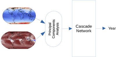
a.	b.

Figure 1: a) Cascade Network. b) Use for climate model data.

2 Models of Climate Change

The sixth phase of the Coupled Model Intercomparison Project [3] (CMIP6) has produced 35 models of earth’s atmosphere from which simulated global temperature and precipitation maps can be obtained for years from 1850 to 2100. This data can be used to investigate spatial and temporal temperature and precipitation patterns that relate to changes in climate. For example, Barnes, et al. [1, 2], used CMIP5 data to map global temperature data to years. They found that linear models predicted the year quite well. They also recast the regression problem as a classification problem in order to use Layerwise Relevance Propagation (LRP) to identify spatial patterns significant to classifying specific decades [5].

Here the regression approach is extended by including temperature and precipitation CMIP6 data and modeling it with a cascade network. We used this data with a spatial resolution of 120 latitudes and 240 longitudes. Not surprisingly, this data has numerous correlations among spatial locations, which was dealt with in prior work by performing ridge regression to limit the magnitude of weights in the first layer of the neural network models [1]. Here we use an alternative approach—Principal Components Analysis (PCA) is used to represent the data with independent factors and to decrease the data dimensionality, illustrated in Figure 1b.

To reveal patterns in the data that relate to the predicted years, a direct approach is used here. Patterns in global temperature and precipitation to which a trained network is most sensitive are determined by reconstructing the original global maps from the the weights in the first layer of a network.

3 Method

Let $x_{i}$ be the $i^{th}$ input sample that is received by all networks. Let $y_{i,j}=f_{j}(x_{i})$ be the output of the $j^{th}$ network for input sample $x_{i}$. For the regression problems considered here, the target value for the $i^{th}$ sample is the scalar $t_{i}$. As shown in Figure 1a, the sum of the outputs, $Y_{i}=\sum_{j=1}^{M}y_{i,j}$ forms the output of the cascaded nets. The objective is to minimize the sum of squared errors $\sum_{i=1}^{N}(t_{i}-Y_{i})^{2}$.

The optimization problem is structured to encourage the simpler nets, higher in the cascade shown in Figure 1, to reduce the error as much as possible before recruiting a more complex network to reduce the error further. To accomplish this, the target value for net $j$ is the original target minus the sum of the outputs of the previous, simpler networks: the target value, $t^{\prime}_{i,j}$, for input $i$ for net $j$ is $t^{\prime}_{i,j}=t_{i}-\sum_{k=1}^{j-1}y_{i,j}$.

The CMIP6 data consists of simulated annual temperature and precipitation from 35 models for 251 years from 1850 through 2100, at 120 latitudes and 240 longitudes. The mean annual temperatures and precipitations across the globe are removed from each sample. This data is divided into training, validation, and testing partitions selected from different years. The training partition was assigned 50% of the data, and the validation and testing partitions were each assigned remaining 25% of the data. Each partition contained data from all 35 atmosphere models, but for different sets of years. The partitioning can be seen in Figures 2 and 3.

Optimization of the networks is performed on the training partition using the Scaled Conjugate Gradient algorithm [4]. PCA is performed by projecting the flattened and concatenated temperature and precipitation maps onto 1 to 500 principal components. The structures of the neural networks in the cascade structure have increasing numbers of hidden layers, each layer containing only two units having the hyperbolic tangent activation functions. This number of units was found to generalize better to validation and testing data than larger numbers of units.

4 Results

The results of the training procedure are shown in the following figures. Figures 2a and b plot the RMSE in predicted year with respect to the number of principal components (PCs). Each of our data samples contain $120\times 240$ values for temperature and also for precipitation, resulting in 57,600 values. During our training experiments, we tested the use of 1 to 500 PCs, a large reduction in dimensionality of the data. More PCs resulted in higher generalization error.

Figure 2a shows that RMSE for the three data partitions are similar, with the best number of PCs, determined by the lowest validation error, was found to be 240. Figure 2b is a plot of the number of neural nets included in the cascade nets for each number of PCs. With a small number of PCs, the cascade keeps up to 7 nets, but as the number of PCs is increased, fewer nets are needed to maintain a low error. Recall that nets increase in complexity (number of hidden layers) but are kept in the cascade only if their inclusion decreases the validation error. The cascade trained with 240 PCs contains two neural nets, one being the linear net, and one with a single hidden layer.

Figure 2c shows the RMSE in predicted year for the best cascade, the one with 240 PCs. The error for a linear network, with 0 hidden layers, 27 to 30 years. When the single hidden layer net is added to the cascade the error is reduced to 20 to 22 years. Figure 2d shows the predicted year versus the actual year. Perfect prediction would result in all points falling along the red diagonal line. The partitioning of the data into training, validation, and testing subsets is clear in this plot. It is clear that data from later years, from 2000 to 2100 is predicted better by the cascade. Is is also apparent that data for the years from 1850 to about 1950 is harder to predict. Perhaps this is due to a lack of information in the temperature and precipitation maps that are related to specific years in this early period.

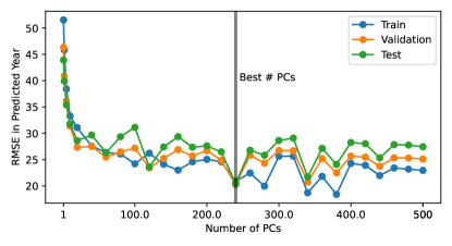
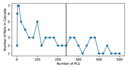
a.	b.
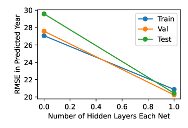
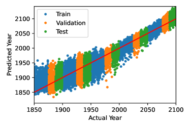
c.	d.

Figure 2: a) RMSE in predicted year versus the number of principal components (PCs). The best number of PCs at 240 is determined by the lowest validation RMSE. b) Number of nets in the cascade model versus number of PCs. c) RMSE in predicted years for the best cascade model due to each of the two nets. d) Predicted year versus the actual year for all samples.

Since the cascade model consists of two networks, one with no hidden layers and one with one hidden layer, an obvious question is whether or not there is a span of years with the second network most helps in predicting the year. Figure 3 shows that the answer is “yes”. This figure shows the RMSE in predicted year versus the actual year for the three data partitions. In each plot the RMSE is shown for just the linear network, then again for the combination of the linear and the nonlinear network with a single hidden layer. The second and third plots, for the validation and test partitions, respectively, show that the addition of the second network with one hidden layer with nonlinear activation functions improves the prediction of the year (decreases the error) for the latest span of years. This suggests that the patterns in the data that the second network have acquired may indicate aspects of the global temperature and precipitation data that distinguish early from late years, and thus help identify climate change indicators.

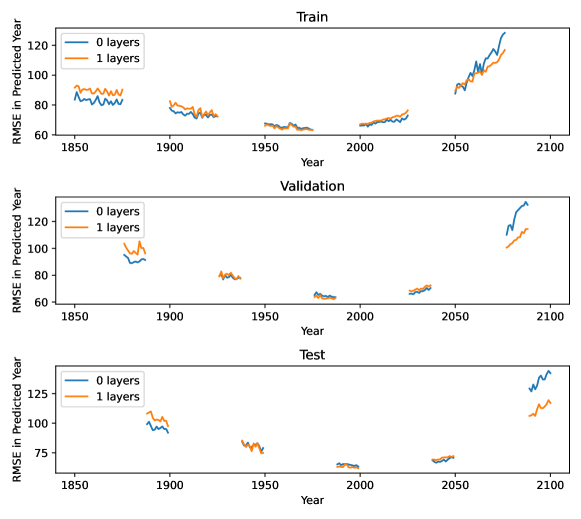
Figure 3: RMSE in predicted year using just the linear network and with the cascade model output that is the combination of the linear network and the one-hidden layer network.

To visualize these patterns, the following procedure was used. The weights in the units of the first layer of a network were used to reconstruct the global temperature and precipitation maps by combining each principal component multiplied by the corresponding weights. Figure 4a shows the result for the linear network. The temperature map is not surprising; indicates that higher temperatures in the arctic are positively related to an increase in year. A closer examination shows that increased temperature in the Barents Sea north of Finland may be more strongly positively related to year. The precipitation map reveals a higher significance in precipitation near the equator as a positive relationship to year.

Figure 4b shows the maps from the two units in the first, and only, hidden layer of the second network. Differences among the temperature maps are not clear, though can be revealed with higher-resolution images. More obvious differences exist in the precipitation maps. It appears that these maps show an asymmetry above and below the equator in positive and negative relationships with year over the Pacific ocean. Another asymmetry appears between precipitation in the Pacific versus the Atlantic oceans. These asymmetries are not apparent in the precipitation map for the linear network. Since the addition of this network lowered the error for the latest years, these maps may reveal key differences in precipitation in late versus early years in the 1850-2100 span.

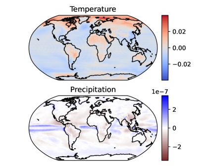
a.

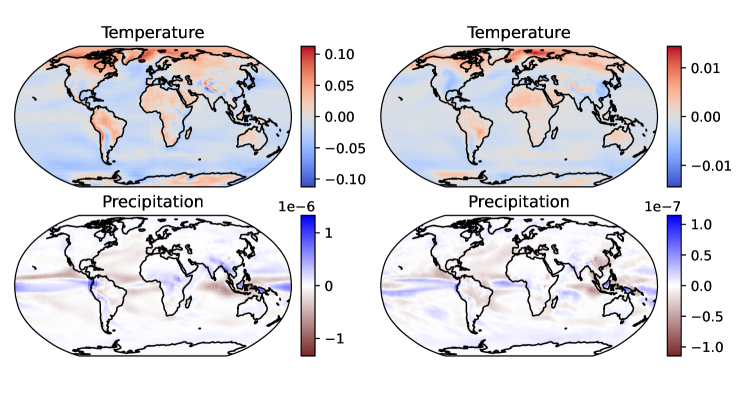
b.

Figure 4: Temperature and precipitation maps related to year. a) Maps from the first linear network. b. Maps from the two units in the single hidden layer of the second network.

5 Conclusion

An ensemble of neural networks is developed in a cascade structure in which simpler networks are trained first and more complex ones, with additional hidden layers, are trained and kept only if they result in lower error on a validation set. The result is a model that can be interpreted by assembling aspects of the data to which each network is learned to be sensitive.

The training of a cascade model of temperature and precipitation changes with respect to year results in correct year prediction with an approximate error of 20 years over the span of 1850 to 2100. The data only supports a single-hidden layer net added to the initial linear net. Additional, more complex nets increase the validation error. Similar increases in validation error occur with larger numbers of principal components used to project the 57,600 to smaller dimensions.

Current experiments with the cascade structure are underway with data sets that contain stronger nonlinearities, and with classification problems.

Acknowledgments

This work was partially funded by NSF Grant #2019758, AI Institute: Artificial Intelligence for Environmental Sciences (AI2ES)

References

- [1] E. A. Barnes, J. W. Hurrell, I. Ebert-Uphoff, C. Anderson, and D. Anderson. Viewing forced climate patterns through an ai lens. Geophysical Research Letters, 46(13):13389–13398, 2019.
- [2] Elizabeth A. Barnes, Benjamin Toms, James W. Hurrell, Imme Ebert-Uphoff, Chuck Anderson, and David Anderson. Indicator patterns of forced change learned by an artificial neural network. Journal of Advances in Modeling Earth Systems, 12(9):e2020MS002195, 2020.
- [3] V. Eyring, S. Bony, G. A. Meehl, C. A. Senior, B. Stevens, R. J. Stouffer, , and K. E. Taylor. Overview of the coupled model intercomparison project phase 6 (cmip6) experimental design and organization. Geosci. Model Dev., 9:1937–1958, 2016.
- [4] M.F. Møller. A scaled conjugate gradient algorithm for fast supervised learning. Neural networks, 6(4):525–533, 1993.
- [5] B. A. Toms, E. A. Barnes, and I. Ebert-Uphoff. Physically interpretable neural networks for the geosciences: applications to earthsystem variability. Journal of Advances in Modeling Earth Systems, 12:e2019MS002002, 2020.