SKYSURF: Constraints on Zodiacal Light and Extragalactic Background Light through Panchromatic HST All-Sky Surface-Brightness Measurements: II. First Limits on Diffuse Light at 1.25, 1.4, and 1.6 microns

Abstract

We present the first results from the HST Archival Legacy project “SKYSURF.” As described in Windhorst et al. (2022), SKYSURF utilizes the large HST archive to study the diffuse UV, optical, and near-IR backgrounds and foregrounds in detail. Here we utilize SKYSURF’s first sky-surface brightness measurements to constrain the level of near-IR diffuse Extragalactic Background Light (EBL) in three near-IR filters (F125W, F140W, and F160W). This is done by comparing our preliminary sky measurements of $>30,000$ images to Zodiacal light models, carefully selecting the darkest images to avoid contamination from stray light. Our sky-surface brightness measurements have been verified to an accuracy of better than $1\%$, which when combined with systematic errors associated with HST, results in sky brightness uncertainties of $\sim 2-4\%\simeq 0.005$ MJy/sr in each image. When compared to the Kelsall et al. (1998) Zodiacal model, an isotropic diffuse background of $\sim 30$ nW m^-2 sr^-1  remains, whereas using the Wright (1998) Zodiacal model results in no discernible diffuse background. Based primarily on uncertainties in the foreground model subtraction, we present limits on the amount of diffuse EBL of 29 nW m^-2 sr^-1 , 40 nW m^-2 sr^-1 , and 29 nW m^-2 sr^-1 , for F125W, F140W, and F160W respectively. While this light is generally isotropic, our modeling at this point does not distinguish between a cosmological origin or a Solar System origin (such as a dim, diffuse, spherical cloud of cometary dust).

1 Introduction

The cosmic optical and near-IR Extragalactic Background Light (EBL), derived from the integrated luminosity of all extragalactic objects over all redshifts, represents a fundamental test of our understanding of extragalactic astronomy (e.g., McVittie & Wyatt, 1959; Partridge & Peebles, 1967a, b; Hauser & Dwek, 2001; Lagache et al., 2005; Kashlinsky, 2005; Finke et al., 2010; Domínguez et al., 2011; Dwek & Krennrich, 2013; Khaire & Srianand, 2015; Driver et al., 2016; Koushan et al., 2021; Saldana-Lopez et al., 2021). If our census of galaxies and their luminosities are truly complete, the total EBL level should equal that of all discrete objects. On the other hand, if the EBL is found to be in excess of predictions from galaxy counts, that suggests that galaxy surveys may be missing some discrete or diffuse sources. Despite the importance of this measurement, direct EBL measurements have yet to arrive at a value that agrees with predictions from galaxy number counts (for a recent review, see Cooray, 2016). Project SKYSURF (Windhorst et al., 2022) aims to study this discrepancy with the vast archive of HST images.

Because of the difficulty of characterizing the foreground signal of Earth’s atmosphere, observational attempts at constraining the EBL level directly are primarily done with space missions, such as COBE (e.g., Puget et al., 1996; Fixsen et al., 1998; Dwek & Arendt, 1998; Hauser et al., 1998; Finkbeiner et al., 2000; Cambrésy et al., 2001; Sano et al., 2020), Spitzer (Dole et al., 2006), HST (Bernstein et al., 2002; Bernstein, 2007), IRTS (Matsumoto et al., 2005, 2011), and AKARI (Matsuura et al., 2011; Tsumura et al., 2013). These observations have large errors and are often discrepant with each other because of the limited number of observations and the difficulty of subtracting the instrumental, Zodiacal, Galactic, and astrophysical foregrounds (Cooray, 2016). Regardless, these direct measurements consistently arrive at EBL levels of $\sim 20-50$ nW/m²/sr, significantly above the predictions from galaxy counts of $\sim 10$ nW/m²/sr (e.g.  Driver et al., 2011; Andrews et al., 2018). Recent advances have been made with the CIBER experiment (Matsuura et al., 2017; Korngut et al., 2022), and Pioneer and New Horizons missions (Matsumoto et al., 2018; Lauer et al., 2021, 2022) that aim to better subtract the Zodiacal foreground, using Ca absorption features and by leaving the solar system, respectively. These observations find EBL levels closer to expectations, but they still identify a significant diffuse signal and represent a relatively small number of measurements. A parallel indirect approach, using observations of attenuated $\gamma$-rays, also finds values in line with predictions from galaxy counts (H. E. S. S. Collaboration et al., 2013).

While the presence of diffuse EBL may diminish as new measurements better constrain foreground levels, many astrophysical sources have been hypothesized as contributing to it. The large population of recently-identified Ultra-Diffuse Galaxies in clusters (Impey et al., 1988; van Dokkum et al., 2015) and the field (Dalcanton et al., 1997; Leisman et al., 2017) represents one possible source of diffuse light, although many more unidentified UDGs would have to be present to contribute significantly to the EBL (Jones et al., 2018). Diffuse light in the outskirts of galaxy halos (IGL) may contribute as well (Conselice et al., 2016), although a number of studies (e.g.  Ashcraft et al., 2018; Borlaff et al., 2019; Cheng et al., 2021) find that halo light, or light in galaxy outskirts, only represents $15\%$ of the luminosity of bright galaxies. Alternatively, significant levels of difficult-to-detect diffuse intracluster (Bernstein et al., 1995) or intragroup light (Mihos et al., 2005) may contribute to the diffuse EBL. More exotic explanations, such as light from reionization (Santos et al., 2002; Cooray et al., 2004; Kashlinsky et al., 2004) have been put forward as well.

The SKYSURF project, introduced in Windhorst et al. (2022), aims to better understand the EBL level with the large volume of archival HST observations using a two-pronged approach. First, it will use HST’s remarkable stability and precision as an absolute photometer to conduct precise sky brightness measurements for over $200,000$ HST images. Second, it will use the depth and large volume probed by those images to search for possible sources of diffuse EBL.

For the full motivation and overview of the SKYSURF project, and an overview of its methods, see Windhorst et al. (2022); we refer to this paper as SKYSURF-1 throughout. In this paper, we describe the first results of SKYSURF surface-brightness measurements at 1.25, 1.4, and 1.6 microns. In Section 1.1 we further outline the diffuse foreground sources necessary to consider for SKYSURF’s EBL constraints, in Section 2, we briefly describe our measurement procedure, Sections 3 presents our results, Section 4 includes a discussion of those results, and Section 5 summarizes our conclusions. Throughout we use Planck cosmology (Planck Collaboration et al., 2016): $H_{0}$  = 66.9 km s^-1 Mpc^-1  , matter density parameter $\Omega_{m}$=0.32 and vacuum energy density $\Omega_{\Lambda}$=0.68. When quoting magnitudes, our fluxes are all in AB-magnitudes (hereafter AB-mag), and our SB-values are in AB-mag arcsec^-2 (Oke & Gunn, 1983) or MJy/sr, using flux densities $F_{\nu}$ = 10${}^{-0.40({\rm AB}-8.90\ {\rm mag})}$ in Jy. Further details on the flux density scales used are given in Fig. 10 and the Table footnotes in § 3.

1.1 Foregrounds

The main goal of SKYSURF is to characterize the components of sky surface brightness present in HST images, including a possible diffuse EBL component, in detail. Below, we summarize the relevant astronomical foregrounds and backgrounds that exist in the SKYSURF images. In summary, they are the following: Zodiacal Light (ZL), Diffuse Galactic Light (DGL), discrete stellar and extragalactic light, and diffuse EBL. The Zodiacal Light (ZL) is the main foreground in most HST images, and SKYSURF will measure and model it as well as possible with available tools. All stars in our galaxy (except the Sun) and all other galaxies are beyond the InterPlanetary Dust Cloud (IPD), so the ZL is thus always referred to as a “foreground”. Similarly, the Diffuse Galactic Light, caused by scattered star-light in our Galaxy, can be a background (to nearby stars), or a foreground (to more distant stars and all external galaxies). Most objects in an average moderately deep (AB$\lesssim$25–26 mag) HST image are faint galaxies close to the peak in the cosmic star-formation history at $z$$\lesssim$$2$ (e.g.  Madau & Dickinson, 2014). Most of the Extragalactic Background Light (EBL) therefore comes from distant galaxies and AGN, and is thus referred to as a “background”.

Before SKYSURF can quantify and model these astronomical foregrounds and backgrounds, it needs to address the main contaminants, which are residual detector systematics, orbital phase-dependent straylight from the Earth, Sun, and/or Moon, and the WFC3/IR Thermal Dark signal. Instrumental and stray light contaminants, as well as the contribution of discrete objects to the SKYSURF EBL constraints, are discussed in SKYSURF-1. Below, we discuss the diffuse Zodiacal, Galactic, and Extragalactic foregrounds in more detail.

1.1.1 Zodiacal Foreground

By far, the brightest component of the sky brightness is Zodiacal Light from the InterPlanetary Dust (IPD) cloud, i.e., from distances less than 5 AU, representing over $95\%$ of the photons with 0.6-1.25 µm wavelengths in the HST archive (see Fig. 10). Given its extremely diffuse nature, as well as its time variability, it has been a challenge to understand in detail; observations with all-sky space missions such as COBE/DIRBE are required to fully model it. For example, the Kelsall et al. (1998) and Wright (1998) Zodiacal models use the COBE/DIRBE data to model the Zodiacal emission, considering multiple dust components scattering sunlight toward Earth. The absence of an all-sky optical survey means that such modeling cannot be done in the optical to a similar extent; most authors simply assume that the Zodiacal spectrum is a Solar, or slightly reddened Solar spectrum (e.g., Leinert et al., 1998). Future SKYSURF studies will utilize its UV-to-optical database to improve constraints on the Zodiacal spectrum, but here we only consider observations with wavelengths similar to COBE/DIRBE wavebands for which a detailed Zodiacal model is obtainable.

1.1.2 Discrete and Diffuse Light from Kuiper Belt Objects

The darkness of the night sky, “Olbers’ Paradox”, was one of astronomy’s oldest mysteries: an infinite and infinitely old Universe full of stars and galaxies would have a sky as bright as the surface of an average star. The resolution of this “paradox” — an expanding Universe of finite age — is, of course, the central tenet of Big Bang cosmology, where the galaxy surface density is a finite integral over the galaxy luminosity function and the cosmological volume element (Driver et al., 1995; Metcalfe et al., 1995; Odewahn et al., 1996; Tyson, 1988). Because of their very steep observed number counts, Kuiper Belt Objects (KBOs) can also appear to violate Olbers’ Paradox, producing an apparently diverging sky integral when the smallest objects are taken into account (e.g., Kenyon & Windhorst, 2001). To not exceed the observed the ZL sky-SB, the counts of KBOs at distances $\gtrsim$40 AU must turn over from the non-converging power-law slope $\gamma$$\simeq$0.6 dex/mag observed for R$\lesssim$27 mag (Fraser et al., 2014) to a converging slope flatter than $\gamma$=0.4 dex/mag at R-band fluxes of AB$\gtrsim$45–55 mag, in combination with a limited volume over which KBOs occur (Kenyon & Windhorst, 2001). Assuming albedos of a few percent (e.g., Kenyon & Luu, 1999) and a physical size distribution of $N(r)\propto\ r^{-\beta}$, such a slope change in the KBO number counts implies that the size-slope of unresolved Solar System debris at $\sim$40 AU must flatten from $\beta$$\simeq$4 for larger objects to $\beta$$\lesssim$3.25–3.5 for objects with sizes $r$$\sim$0.05–5 m. A flattening of the size distribution of the planetesimal population with radii $r$$\gtrsim$10 km from $\beta$$\simeq$4 to $\beta$$\lesssim$3.5 is consistent with simulations for the debris population with $r$$\lesssim$1 km, which suggest that collisions with $r$$\lesssim$100 m objects tend to produce debris rather than larger planetesimals (Kenyon & Luu, 1999; Kenyon & Bromley, 2004, 2020). It is also consistent with ground-based observations of KBOs with $r$$\lesssim$50 km (e.g., Fuentes et al., 2009; Shankman et al., 2013), and with New Horizons (NH) crater counts on Pluto and Charon, which suggest a flattening of the KBO count slope for $r$$\lesssim$1 km (e.g., Singer et al., 2019).

To refine these constraints across the Kuiper Belt, SKYSURF will measure the panchromatic Zodiacal foreground in the ecliptic plane in places where other foregrounds are small. Better SB-limits on the small KBO population may constrain the slope of the KBO counts, and hence the total Kuiper Belt mass at 35–50 AU. Time-tagged monitoring of the sky-SB in the Ecliptic may also yield constraints to the integral of Plutinos in Neptune’s L4 and L5 Lagrange points, which have moved significantly in Ecliptic Longitude ($l^{\rm Ecl}$) during the 32-year HST mission. Kelsall et al. (1998) fit the data from the Cosmic Background Explorer/Diffuse InfraRed Background Experiment (COBE/DIRBE) as a family of 3-D (flaring) disk models of decreasing density with increasing radius and distance from the ecliptic plane. This model accounts for the variation with Solar phase angle for realistic properties of dust grains. Other ZL models and refinements were presented by, e.g., Reach et al. (1997), Leinert et al. (1998), Wright (1998), Wright (2001), Jorgensen et al. (2021), Arendt (2014), and Arendt et al. (2016). Kelsall et al. (1998) adopt an albedo at 1.25 µm wavelength for their Zodiacal “Smooth Cloud”, “Dust Bands”, and “Ring+Blob” components of $a$=0.204$\pm$0.0013. Recent thermal IR observations of Trans-Neptunian Objects (TNOs) with typical sizes of $\sim$20–400 km imply geometric albedo values of $\lesssim$20–30%, whereas TNOs have albedos as large as $\sim$60% (e.g., Duffard et al., 2014; Kovalenko et al., 2017; Vilenius et al., 2012, 2014, 2018), possibly indicating a more icy surface for some TNOs. Possible variation in Solar System objects, and the impact that they may have on our results is discussed further in § 4.

1.1.3 Diffuse Galactic Light

Diffuse Galactic Light (DGL) in the UV–optical is mainly caused by scattered light or reflection nebulae from early-type (O and B) stars, scattered by dust and gas in the Interstellar Medium (ISM). The DGL is thus a strong function of Galactic coordinates ($l^{II}$, $b^{II}$). SKYSURF’s SB-measurements may thus also constrain the DGL at low Galactic latitudes ($b^{\rm II}$ $\lesssim$20–30^∘), although these fields are very likely not useful for background galaxy counts. The All-sky Infrared Astronomical Satellite (“IRAS” Soifer et al., 1984; Helou & Walker, 1985), COBE/DIRBE (Kelsall et al., 1998; Schlegel et al., 1998), Planck (Planck Collaboration et al., 2016), Wide-field Infrared Survey Explorer (WISE; Wright et al., 2010), and AKARI (Tsumura et al., 2013) maps in the near to far-IR help identify Galactic infrared cirrus and regions of likely enhanced Galactic scattered light. Possible high spatial frequency structures in the DGL appear in deep ground-based images of low Galactic latitude at SB-levels of B$\simeq$26–27 mag/arcsec², and at much fainter levels sometimes also at high Galactic latitudes (e.g., Szomoru & Guhathakurta, 1998; Guhathakurta & Tyson, 1989). While not a main goal of SKYSURF, the DGL needs to be estimated and subtracted in order to better estimate the levels of the ZL and the EBL at higher Galactic latitudes, as discussed in § 3. Panchromatic HST constraints on the DGL in the Galactic plane ($|$$b^{II}$$|$$\lesssim$20^∘) are interesting in their own right and are a byproduct of SKYSURF. We refer to § 3.5 for the DGL levels we subtract from any diffuse light levels implied by the comparison between our HST sky-SB measurements and the ZL models.

2 Measurements

An overview of the SKYSURF database and our sky measurement procedure can be found in SKYSURF-1. Further details on the multiple sky measurements procedures, as well as the full results of the sky surface brightness measurements across the entire SKYSURF database will come in O’Brien et. al. (2022, in preparation). For context, we give a brief overview of the database and methods here.

First, the HST archive was searched for images taken with its wide-band filters, excluding grism images, quad/linear ramp or polarizing filters, subarray images, time-series, moving targets, or spatial scans. This resulted in $249,861$ images that made up the initial database. Further cuts on target selection, HST orbital phase, and exposure time will be conducted to avoid possible contamination and minimize measurement errors.

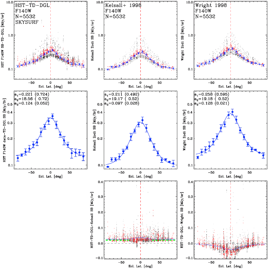
Figure 8: [(a) Top Left]: HST WFC3/IR sky-SB measurements in the F140W filter vs. Ecliptic Latitude after subtracting the best WFC3/IR Thermal Dark signal estimate for each exposure from § 3.3 and the Diffuse Galactic Light (DGL) signal from § 3.5. Black dots indicate all observations from Fig. 2, and red dots only those with Sun Angle SA=90$\pm$10^∘. The COBE/DIRBE data, to which the models were fit, were taken at a comparable SA-range. The blue points indicate the one-sided clipped medians of the SA=90$\pm$10^∘ points in each 10^∘ $b^{\rm Ecl}$-bin, and the blue line indicates the best $sech$-fit to these medians. [(b) Top Middle]: Kelsall et al. (1998) ZL model prediction for the same sky pointings and filters, observing day of the year, and Sun Angles as the HST data in (a) with their medians and best fit $sech$-model. [(c) Top Right]: As in (b), but for the Wright (1998) Zodiacal model prediction. [(d), (e), (f) Middle Row]: The clipped medians for each $b^{\rm Ecl}$-bin from panels (a), (b), (c) are reproduced for clarity, respectively, with their errors plus the best $sech$-fits and their coefficients. [(g) Bottom Middle]: Difference between each (HST–TD–DGL) data point from (a) and its Kelsall et al. (1998) ZL model prediction from (b), with the difference in their $sech$-fits (blue line). The green dashed line indicates the two-sided 1-sigma clipped median for SA=90$\pm$10^∘ and $|$$b^{\rm Ecl}$$|$$\gtrsim$30^∘ (Table 3). [(h) Bottom Right]: As in (g), but for the Wright (1998) Zodiacal model prediction from (c).

To measure the sky background of these images, the SKYSURF team tested multiple sky-measurement algorithms on realistic simulated images to identify the most robust method of estimating the uncontaminated sky background. All algorithms that were tested had an accuracy of better than $0.2\%$ for flat images, and slightly worse for images with gradients (Fig. 8 in SKYSURF-1, ). At this point, it is worth identifying the general philosophy of the SKYSURF program as to identify the Lowest Estimated Sky (LES) value — defined as the lowest sky-SB in an image — as the fiducial sky measurement. While electronic errors within the cameras can introduce either positive or negative errors in sky estimation, errors deriving from contamination (i.e. stray light from nearby bright sources like the Earth and the Sun or thermal emission from the telescope) are more common and more significant. To make full use of our large dataset, we aimed to develop and use algorithms that are the most robust across our database, which contains a wide variety of images. The full results with the most robust algorithms will be presented in O’Brien et. al. (2022, in preparation); here we present the first results using an initial estimation done by fitting a Gaussian to the sigma-clipped image (described as method 2 in O’Brien et. al. (2022, in preparation) and SKYSURF-1).

Combining the sky measurement uncertainties with the systematic uncertainties associated with HST’s detectors, the overall absolute uncertainty on the sky measurements is $\sim 2.7\%$ for the F125W, $\sim 2.8\%$F140W, and $\sim 3.8\%$ for the F160W filter. The systematic uncertainties come from Bias/Darkframe subtraction ($\lesssim 1.0\%$), the global flat field correction ($0.5-2\%$), zeropoint accuracy ($\sim 1.5\%$), and thermal dark subtraction ($\sim 0.2\%$ for F125W, $0.5\%$ for F140W, and $\sim 3.8\%$ for F160W).

3 First SKYSURF Results on Diffuse Near-IR Sky-SB Estimates at 1.25–1.6 µm

For the final analysis of 249,861 SKYSURF images, we expect $\lesssim$50% to be usable for sky-SB measurements. Although these images are not completely randomly distributed on the sky, they on average provide $\sim$4400 sky-SB measurements in each of the 28 broad-band SKYSURF filters. In this section, we will use two complementary analyses of the HST sky-SB estimates to make our first assessment of available Zodiacal Light models, identify any diffuse light that may be present, and check on the consistency of our methods.

The results from both methods will be compared to the Kelsall et al. (1998) and Wright (1998) models, which predict the ZL brightness as a function of sky position and time of the year. Both Kelsall et al. (1998) and Wright (1998) models are fit to COBE/DIRBE measurements at $1.25-2.2\leavevmode\nobreak\ {\micron}$. Kelsall et al. (1998) is a physical model that contains multiple dust components, whereas the Wright (1998) model is a more parametric model normalized at $25$ µm to ensure $0$ residual diffuse light at the ecliptic poles. Because their ZL model predictions are anchored to the COBE/DIRBE 1.25–2.2 µm data, we will limit our analysis in this paper to the SKYSURF WFC3/IR filters F125W, F140W, and F160W. We will deal with the uneven sky-sampling of the HST data by comparing the HST sky-SB data with the corresponding ZL model predictions. Again, our premise throughout is that the lowest estimated sky-SB values measured amongst the HST images in each direction will be the least affected by HST systematics or discrete foreground objects, and therefore be closest to the true sky-SB in that direction.

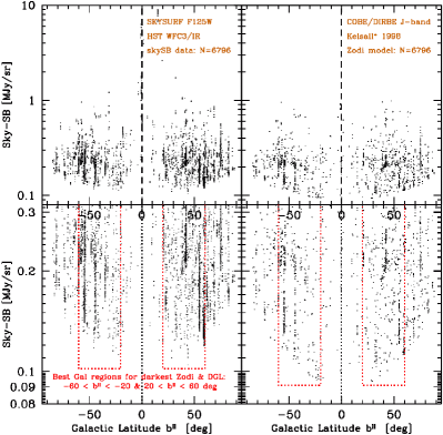
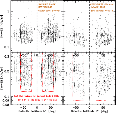
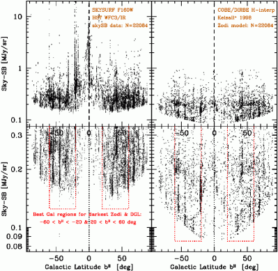
Figure 1: All SKYSURF F125W, F140W, and F160W sky-SB measurements vs. Galactic Latitude for the HST data [left sub-panels] and the Kelsall et al. (1998) COBE/DIRBE models [right sub-panels]. The upper left plot is for F125W, the upper right plot is for F140W, and the lower left plot is for F160W. All bottom sub-panels are enlargements of top sub-panels. Because of the $\sim$60^∘ tilt of the Galactic plane with respect to the Ecliptic, the darkest sky-SB occurs for 20^∘$\lesssim$$|$$b^{II}$$|$$\lesssim$60^∘, highlighted by the red columns in all bottom sub-panels. Fields with $|$$b^{II}$$|$$\lesssim$20^∘ have significant DGL, and are ignored in the final sky-SB analysis.

The first approach uses the Lowest Estimated Sky-SB values from the HST images. Both the HST LES-data and the Kelsall et al. (1998) model predictions are fit with analytic functions as a function of Ecliptic Latitude ($b^{Ecl}$) in the darkest parts of the Galactic sky. These fits will be referred to as the Lowest Fitted Sky-SB (“LFS”) method. To avoid regions with significant DGL, the LFS method will first select the LES-data and model predictions as a function of Galactic Latitude ($b^{II}$), to identify the darkest regions of the Galactic sky.

Next, the LFS method will identify the lowest sky-SB as a function of Ecliptic Latitude ($b^{Ecl}$) to constrain the ZL+EBL sky-SB in each direction (see Fig. 2). For $|$$b^{II}$$|$$\gtrsim$20^∘, where the DGL contribution is lower, the LFS fits provide analytical functions describing the lowest sky-SB as a function of Ecliptic Latitude for both the HST data and the model predictions in the same directions of the sky. The limitation of the LFS method is that not all sky-SB measurements are done at constant Sun Angles (SA; defined as the Sun-HST-target angle), which ranges from SA$\simeq$85–180^∘ at the Ecliptic to SA=90^∘ at the Ecliptic poles. Although many HST observations are scheduled around SA$\sim 90$^∘, many others are done with higher solar elongations for which the Zodiacal sky-SB is lower (the Zodiacal sky-SB reaches a minimum in the Ecliptic at Solar Elongations of 120–150^∘ (Leinert et al., 1998)). This method will thus focus on observations with SA$\sim$150^∘ in the Ecliptic Plane and SA$\sim$90^∘ at the Ecliptic Poles. However, because the analysis is conducted on the Zodiacal models in parallel, this is not expected to bias our results. In particular, this method aligns with the SKYSURF philosophy that most sources of error are positive, and thus the lowest sky values are likely the most accurate.

The second method more closely follows the actual selection of the COBE/DIRBE data, on which both the Kelsall et al. (1998) and Wright (1998) models were based. The COBE/DIRBE data were measured at Sun Angles SA$\simeq$94$\pm$30^∘ (e.g., Leinert et al., 1998). The HST data are observed over a range of Sun Angles, but a significant fraction is also observed at SA$\simeq$90$\pm$10^∘, i.e., over a Sun Angle range similar to, but somewhat narrower than that of the COBE/DIRBE data. Hence, our second method will only select the HST LES-data and COBE/DIRBE-based model predictions in the Sun Angle range of SA$\simeq$90$\pm$10^∘. This “SA90 method” has the advantage of the selected HST data being more directly comparable to the COBE/DIRBE based models, but because of their SA-selection, it may also have somewhat higher levels of (unrecognized) Earthshine. The HST data from the SA90 method may thus be systematically somewhat higher than the minimum Zodiacal sky-SB level that is traced with the LFS-method.

Stated differently, the LFS method fits a ($sech$) function to the lowest sky-SB levels observed at each Ecliptic latitude, and is thus based on fewer data points. The LFS method is therefore more reliable, but statistically less precise than the SA90 method. The SA90 method fits regions with sky-SB more comparable to the COBE/DIRBE SA-range, and thus has better statistics in this SA-range, but also subject to higher straylight levels. A comparison between the two methods will then give us an assessment of the uncertainties in any remaining diffuse light. In this initial analysis, as we are simply looking for a possible diffuse excess above the Kelsall et al. (1998) and Wright (1998) models, these approaches work well. Future SKYSURF analysis will investigate stray-light contamination, as well as the structure of offsets between SKYSURF sky values and model predictions, in more detail.

3.1 HST 1.25–1.6 µm Sky-SB Measurements Compared to COBE/DIRBE Predictions

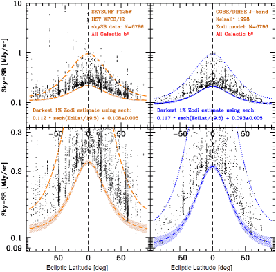
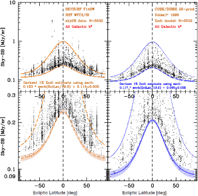
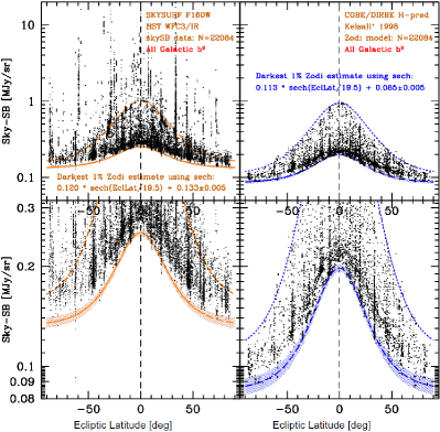
Figure 2: All SKYSURF F125W, F140W, and F160W sky-SB measurements vs. Ecliptic Latitude for HST data (left sub-panels) and the Kelsall COBE/DIRBE models (right sub-panels). The orange and blue $sech$ functions and error wedges outline the darkest $\sim$1% of the sky-SB measurements (magnify the PDF figure as needed to see this). Bottom sub-panels give enlargements of the top sub-panels. As in Figure 1, the upper left plot is for F125W, the upper right plot is for F140W, and the lower left plot is for F160W. The short-dashed blue line represents the upper envelope to the Kelsall et al. (1998) model predictions, and the long-dashed orange line the correspondingly scaled upper envelope to the HST data that does not suffer excessive DGL or straylight, as described in § 3.1 and Table 1.

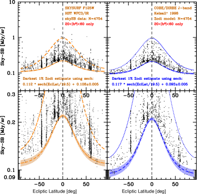
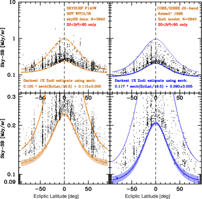
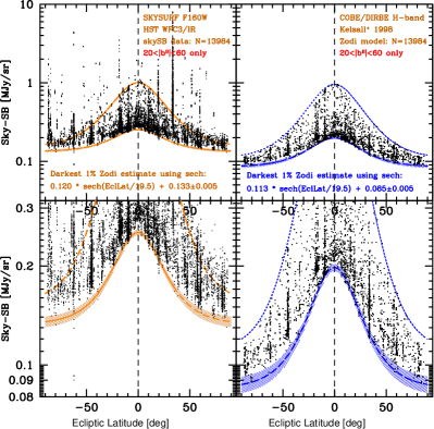
Figure 3: All SKYSURF sky-SB measurements vs. Ecliptic Latitude for HST data (left sub-panels) and the Kelsall COBE/DIRBE models (right sub-panels), but only for the darkest Galactic regions with 20^∘$\lesssim$$|$$b^{II}$$|$$\lesssim$60^∘ (see Fig. 1). As in Figure 1, the upper left plot is for F125W, the upper right plot is for F140W, and the lower left plot is for F160W. The orange and blue $sech$ functions and error wedges outline the darkest $\sim$1% of the sky-SB measurements (magnify the PDF figure as needed to see this). Bottom panels give enlargements of the top panels.

In this section, we present our first SKYSURF results from 34,412 images observed in the WFC3/IR filters F125W, F140W, and F160W. Figs. 1 and 2 show the sky-SB in F125W, F140W, and F160W as a function of Galactic Latitude and Ecliptic Latitude. In these Figures, we simply attempt to find the minimum sky-SB signal in the darkest parts of the sky.

For example, in Fig. 1a the sample of WFC3/IR sky-SB measurements is first plotted vs. Galactic Latitude to find and exclude the regions with significant DGL. Fig. 2 and Fig. 3 then plot the sky-SB vs. Ecliptic Latitude to find in this subset the regions with the lowest LES values of all images in each $b^{\rm Ecl}$-bin. Next, Fig. 1b plots the predictions of the 1.25 µm sky-SB for all HST locations in the sky and at the same Sun Angles at the time of the HST observations as provided by the Zodiacal COBE/DIRBE model of Kelsall et al. (1998). Given the large range in sky-SB values, and the fact that most of the relevant information is at the low-end of the SB-range in all these Figures, the bottom panels in Fig. 1cd provide enlargements of the top panels in Fig. 1ab.

The WFC3/IR ZPs used in the F125W, F140W, and F160W filters are 26.232, 26.450, 25.936 AB-mag, respectively, for an object with 1.000 $e^{-}$/pixel/sec. Fig. 4 shows the HST WFC3/IR F125W  and the COBE/DIRBE J-band total system responses  compared to the Solar spectrum in $F_{\nu}$ (e.g., Arvesen et al., 1969) , which is fairly flat across both these filters. From this, we calculate that for a Solar type spectrum like the ZL that the $\Delta$(HST data–Kelsall COBE/DIRBE model) flux is –0.0061 AB-mag due to the small J-band filter differences. This was calculated three independent ways: using integration in $F_{\lambda}$, pysynphot, and black body interpolation between the two very similar filters, resulting in a scaling factor of HST/Kelsall = 1.00557$\pm$0.0008. That is, for an SED with a Zodiacal spectrum, the HST 1.25 µm fluxes will be $\sim$0.56% brighter than in the COBE/DIRBE J-band filter. Hence, we will multiply the Kelsall et al. (1998) model predictions, which are based on COBE/DIRBE observations, by 1.00557 to bring them onto exactly the same J-band flux scale as the HST WFC3/IR F125W filter for a Solar type spectrum. ZL model predictions for the HST WFC3/IR F140W and F160W filters were derived by interpolation between the Kelsall et al. (1998) COBE/DIRBE J-band and K-band predictions using the slope of the slightly reddened near-IR Zodiacal spectrum of Aldering (2001), with uncertainties that include the errors in the Kelsall et al. (1998) model. While HST and COBE are at different orbits, MSISE-90 Upper Atmospheric models of the Earth  list that the mean atmospheric pressure is 2.27$\times$10^-7 Pa at 540 km and 1.04$\times$10^-8 Pa at 885 km, so it is unlikely that the differences in altitudes between HST and COBE contribute significantly to systematic differences in sky-SB levels between the two missions.

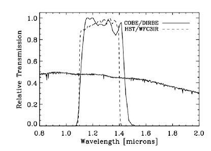
Figure 4: A comparison of the HST F125W and COBE/DIRBE J-band filters, and the to Solar spectrum in $F_{\nu}$, which is fairly flat across these filters. For a Zodiacal spectrum, the expected J-filter flux difference between HST WFC3/IR measurements and the COBE/DIRBE models due to small differences in their respective filter efficiency curves corresponds to –0.0061 AB-mag. We apply this ZP difference to our diffuse light estimates in the Tables of § 3.1. Note that the Geocoronal 1.083 µm He II line is essentially suppressed in the wing of both filters.

Because of the $\sim$60^∘ inclination of the Galactic plane with respect to the Ecliptic, the darkest sky-SB occurs for 20^∘$\lesssim$$|$$b^{II}$$|$$\lesssim$60^∘ and not at the Galactic poles. Fields with $|$$b^{II}$$|$$\lesssim$20^∘ have significant DGL, and are ignored in the analysis of § 3.1–3.4. Fig. 2 shows all HST WFC3/IR F125W, F140W, and F160W sky-SB measurements as in Fig. 1, but now plotted vs. Ecliptic Latitude. The orange and blue sech functions and their error wedges outline the dimmest 1% of the sky-SB measurements as described below. Fig. 3 show the SKYSURF F125W, F140W, and F160W sky-SB values vs. Ecliptic Latitude as in Fig. 2, but only for the darkest Galactic regions with 20^∘$\lesssim$$|$$b^{II}$$|$$\lesssim$60^∘ as selected from Fig. 1.

Natural fits to galaxy disks seen edge-on are $sech$($z$) functions (e.g., van der Kruit, 1988; de Grijs et al., 1997), written as SB in AB-mag vs. vertical distance $z$ from the edge-on disk’s central plane:

$$SB\ =\ a_{4}\ -2.5\ log\ [a_{1}\ sech\ (z/a_{2})\ +\ a_{3}].$$ (1)

According to these authors, the $sech$ model provides a better fit to the vertical or $z$-direction SB-distribution of flattened or ellipsoidal light-distributions seen edge-on than cosine, Gaussian, exponential, single, or squared hyperbolic secant functions. The IPD cloud has a number of modeled components that Kelsall et al. (1998) identify as “Cloud”, “Bands”, and “Ring” around the Sun, within which the Earth orbits. These Zodiacal components have a ratio of their size in the Ecliptic plane to their vertical Ecliptic Height of approximately 4:1, i.e., a rather flattened or “edge-on” distribution as viewed from the Earth. As we will see, $sech$-functions describe the vertical ZL distribution as a function of Ecliptic Latitude as observed from the Earth remarkably well.

Inspired by the work that resulted in Eq. 1, we will use $sech$-type functions to describe the LFS as a function of Ecliptic latitude $b^{\rm Ecl}$. While the actual dependence of ZL brightness with $b^{\rm Ecl}$may be more complicated than Eq. 1 in reality (notably having a significant Sun Angle dependence as discussed below), we find that Eq. 1 is a good description of the dimmest 1% of the sky-SB values for both the HST sky-SB measurements and the Kelsall et al. (1998) model predictions. Furthermore, this fitting procedure allows us to focus on the lower envelope of measurements, which we assume are the least affected by straylight. By repeating the same fitting procedure on the lowest 1% of the Kelsall et al. (1998) model predictions, which predict the ZL brightness for the same direction and at the same time of the year as the HST sky-SB measurements, we can search for any systematic offset between HST measurements and the Kelsall et al. (1998) predictions. This offset could be, an additional unrecognized Thermal Dark component (§ 3.3), a dim spherical or mostly spheroidal Zodiacal component not present in the model, or a dim spherical diffuse EBL component, or some combination of these possibilities.

In the case of HST F125W, F140W, and F160W sky-SB measurements, we use the following $sech$ functions that are simpler than Eq. 1 and linear in flux density to represent the lowest 1% envelope of both the HST data and the Kelsall et al. (1998) models in Fig. 2 & 3. The LFS of the HST data is best represented by:

$$LFS\ (HST)\ =a_{1}(HST)\ sech\ (b_{Ecl}\ /\ a_{2}(HST))\ +\ a_{3}(HST)\ \ \ [MJy/sr],$$ (2)

while the lowest 1% envelope of the COBE model predictions by Kelsall et al. (1998) is best represented by:

$$LFS\ (Kelsall)\ =a_{1}(Kel)\ sech\ (b_{Ecl}\ /\ a_{2}(Kel))\ +\ a_{3}(Kel)\ \ \ [MJy/sr].$$ (3)

Here, $a_{3}$ is the plateau value that the $sech$ function attains when $b^{\rm Ecl}$ reaches $\pm$$\infty$. Next, $a_{1}$ is a constant that captures the maximum vertical amplitude that the $sech$ function reaches at $b^{\rm Ecl}$=0^∘ above this plateau. Last, $a_{2}$$\simeq$19.5^∘ measures the effective thickness of the Zodiacal disk (or “vertical scale height”) as seen edge-on from HST. Coefficient $a_{4}$ in Eq. 1 is a constant that converts the SB in MJy/sr to AB mag arcsec^-2, and is not used in the linear flux density representation of Eq. 2–3. The best estimate parameters of the $sech$ constants $a_{1}$, $a_{2}$, and $a_{3}$ are given in Table 1 for both the lower envelope to the HST data and the Kelsall models at 1.25–1.6 µm. The upper and lower $sech$ envelope $a_{2}$ values are best determined from F160W measurements, which have the best statistics, so we adopt the same $a_{2}$ values and their errors for the F125W and F140W filters in Table 1, which seem to bound the Kelsall et al. (1998) model predictions well for the F125W and F140W measurements. These $sech$ functions are indicated by the bottom orange and blue lines plus their uncertainty wedges in Fig. 2-3, respectively. The main result we are after in Table 1 is the (boldfaced) difference in the bottom envelopes (or $a_{3}$-values) between the HST data and the ZL models. Because the best fit $a_{1}$ and $a_{2}$ values turn out to be very similar in Table 1 for both the HST data and the ZL models, we adopt the differences in $a_{3}$-values as a direct measure of the HST-ZL model differences.

The first four lines of Table 1 also list the same $a_{1}$–$a_{3}$ parameters (and their estimated uncertainties) for the upper envelope to the Kelsall models in the right-most panels, and for the HST data in the left-most sub-panels of Fig. 2-3 (upper blue and orange dashed lines, respectively). The $sech$ upper envelope to the Kelsall et al. (1998) models was directly estimated from the predictions in Fig. 2-3, which show a very good empirical $sech$-type fit to the upper envelope of the Kelsall et al. (1998) model values.

The amplitude of the upper envelope to the HST data was scaled upward using the (HST–Kelsall) difference from the lower envelopes in Fig. 2 and Table 1. The orange dashed lines indicating the upper envelopes to the HST data in Fig. 2a thus provide another way to identify HST exposures with excessive sky-SB, which could be due to several reasons: (a) targets with higher DGL; (b) large nearby galaxy targets, such as the LMC or M31; or (c) exposures with higher straylight levels, including those that got too close to the Earth’s limb. The presence of such images is most noticeable in the F160W filter.

Fig. 5 shows a comparison of SKYSURF’s F125W, F140W, and F160W sky-SB measurements from the HST data to the Kelsall COBE/DIRBE models as a function of Ecliptic Latitude (the top sub-panels show all data, and bottom sub-panels only for the darkest Galactic regions at 20^∘$\lesssim$$|$$b^{II}$$|$$\lesssim$60^∘ as selected from Fig. 1). The left sub-panels give the HST/Kelsall model flux density ratio, while the right sub-panels give the linear flux density difference between the HST data and the Kelsall COBE/DIRBE models for the same subsample. In the top sub-panels of Fig. 5, the orange sech functions in Eq. 2–3, and their error wedges outline the darkest sky-SB measurements from Fig. 2. The bottom sub-panels of Fig. 5 give enlargements of the top sub-panels, and show a significant Ecliptic Latitude dependence of the HST/Kelsall model flux ratios, suggesting that the difference between the bottom envelopes of the HST data and the Kelsall models are not due to a flux density scale issue.

The green wedges in the bottom right panels of Fig. 5 indicate our best estimate of the $\Delta$(HST–Kelsall) offsets. For each filter, these linear flux density differences between the bottom envelopes of the HST data and the Kelsall models are fairly constant for $|$$b^{II}$$|$$\gtrsim$20^∘ and well above zero, suggesting a somewhat wavelength-dependent constant linear offset between the bottom envelopes of the HST data and the Kelsall models. For $|$$b^{II}$$|$$\lesssim$20^∘, the differences between the data and model have more scatter, suggesting that complex and subtle adjustments to the Kelsall model in the ecliptic plane may be required. We thus discard all data with $|$$b^{II}$$|$$\lesssim$20^∘ to estimate the LFS difference between the HST data and Kelsall models.

The LFS values from Fig. 1 are summarized in Table 1. For example, Table 1 shows that the plateau value $a_{3}$ of the $sech$ function in Eq. 2–3 that best captures the LFS values at high Ecliptic Latitudes in the F125W filter amounts to $a_{3}$(HST) = +0.108$\pm$0.005 MJy/sr, which best fits the lowest $\sim$1% of the sky-SB values, while for COBE/DIRBE model predictions for the same sky pointings and filters, observing day of the year, and Sun Angles, the Kelsall et al. (1998) model predicts a lowest $\sim$1% envelope with $sech$ parameter $a_{3}$(COBE) = +0.093$\pm$0.006 MJy/sr. The most likely HST–Kelsall difference from Fig. 5d is thus $\sim$(0.108–0.093*1.0056)$\simeq$+0.0145$\pm$0.008 MJy/sr, which includes the correction for the –0.0061 mag ZP difference between the HST F125W and COBE/DIRBE J-band flux scales. Similar but somewhat larger values are listed in Table 1 for the F140W and F160W filters, where the Kelsall et al. (1998) models were interpolated between the COBE/DIRBE predictions at 1.25 and 2.2 µm following the discussion in § 3.2. This interpolation also results in somewhat larger $a_{3}$ errors for the lower envelope to the Kelsall et al. (1998) model predictions in the F140W and F160W filters in Table 1 (see §3.2), and in somewhat larger errors of $\sim$0.009 MJy/sr in the F140W and F160W HST–Kelsall difference signal listed in Table 1.

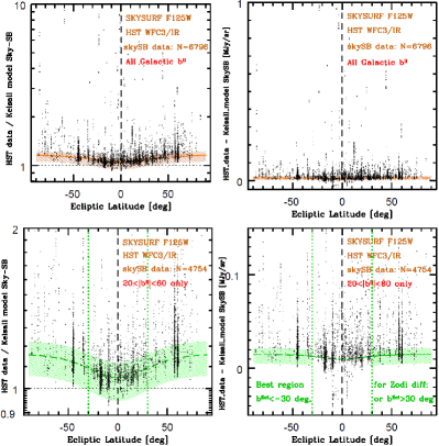
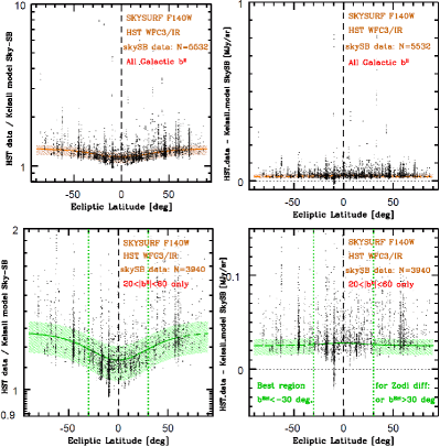
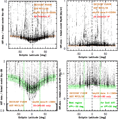
Figure 5: SKYSURF F125W, F140W, and F160W sky-SB measurements from the HST data compared to the Kelsall COBE/DIRBE models [in Myr/sr] vs. Ecliptic Latitude $b^{\rm Ecl}$. Data in the bottom sub-panels is restricted to the darkest Galactic regions with 20^∘$\lesssim$$|$$b^{II}$$|$$\lesssim$60^∘ (see Fig. 1) and zoomed into the most relevant range. Left sub-panels give the HST F125W/Kelsall 1.25 µm model flux density ratio, while the right sub-panels give the linear flux difference between the HST data and the Kelsall COBE/DIRBE models for the same subsample. The orange $sech$ functions and error wedges outline the darkest sky-SB measurements from Fig. 2. The green wedges in the bottom sub-panels illustrate the HST-Kelsall difference between sech fits from Figure 3, highlighting our best estimate of the $\Delta$(HST data – Kelsall COBE/DIRBE model) of 0.0145 $\pm$0.007 MJy/sr for F125W, 0.025 $\pm$0.010 MJy/sr for F140W, and 0.048 $\pm$0.010 for F160W (Table 1). The bottom right sub-panels best capture the linear SB-difference between the HST sky-SB observations and the COBE/DIRBE Kelsall 1.25 µm model (magnify the PDF figure as needed to see the difference).

3.2 Interpolating the Zodiacal Spectrum for F140W and F160W Observations

To estimate Kelsall model predictions for F140W and F160W observations, as well as the thermal modeling described in §3.4.1, a model of how the Zodiacal spectrum behaves in the near-IR is necessary. For short-wavelength IR images (up to 2.2 µm), the sky-SB SED closely resembles a power law in the form of:

$$log(F_{\lambda})\ =\ -17.755-\alpha\ (\lambda-0.61{\micron})\ \ \ \ [erg/cm^{2}/s/\AA/arcsec^{2}]$$ (4)

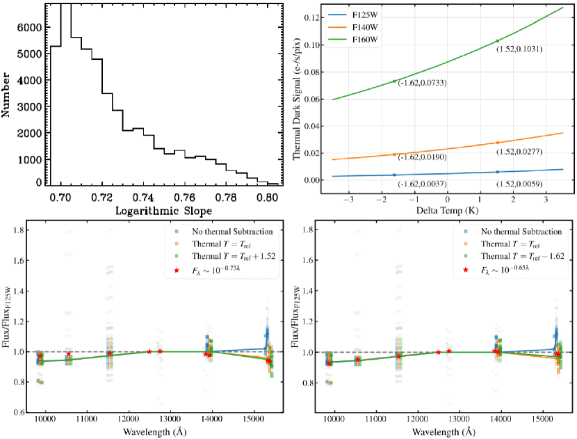
Figure 6: (a) [Top Left]: Spectral index distribution N($\alpha$) when interpolating the Kelsall et al. (1998) Zodiacal sky-SB prediction of SKYSURF F160W pointings in the COBE/DIRBE J and K-band filters. The median power-law spectral index and its 1$\sigma$ range is $\alpha$=0.713$\pm$0.023. (b) [Top Right]: Thermal Dark signal corrections predicted by $synphot$ in the WFC3 F125W, F140W, and F160W filters as a function of the change in telescope ambient temperature $\Delta$T required to provide a best fit to the observed Thermal Dark signals shown in panels (c) and (d). The ($\Delta$T, TD signal) numbers listed bracket the range of temperature and TD signal considered here (see Table 2). (c) [Bottom Left]: Mean Sky-SB values averaged over 500 WFC3/IR exposures in the filters F098M, F105W, F110W, F125W, F127M, F139M, F140W, F159M, and F160W taken in distinct fields, subtracting various different Thermal Dark signal scenarios as a function of ambient temperature $T_{\rm ref}$. The lightly shaded points were affected by the Geocoronal He II 1.083 µm-line (in F105W and F110W), or got too close to the Earth’s limb. The red asterisks show the Zodiacal spectrum of Aldering (2001) at each filter’s effective central wavelength using Eq. 4. All $synphot$ Thermal Dark subtracted scenarios are normalized to the ratio at 1.25 µm, which is by definition unity. Blue squares and their median fit (blue solid line) assume that no Thermal Dark signal needs to be subtracted. The orange squares and green line assume T=$T_{\rm ref}$ as the best fit, which is taken from the reference files. The green squares and green line assume the Aldering (2001) near-IR Zodiacal spectral slope of $\alpha$=0.73 and an HST temperature T=$T_{\rm ref}$ + 1.52 K. (d) [Bottom Right]: As in panel (c), but with the green squares and green line assuming a near-IR Zodiacal spectral slope $\alpha$=0.65 and an HST temperature of T=$T_{\rm ref}$ –1.62 K. The two $\Delta$T cases in panels (b)–(d) bracket the likely range in HST telescope ambient temperatures, which are used to estimate the possible range in F125W–F160W Thermal Dark signal that needs to be subtracted from any diffuse sky-SB signal (§ 3.4).

following Aldering (2001), who adopted a power-law slope $\alpha$=0.730 for wavelengths 0.61$\lesssim$$\lambda$$\lesssim$2.20 µm. Hence, in our analysis, we will use Eq. 4 to represent the Zodiacal spectrum for 0.61$\lesssim$$\lambda$$\lesssim$2.20 µm. Fig. 6a shows the spectral index distribution N($\alpha$) when interpolating the Kelsall et al. (1998) Zodiacal sky-SB prediction in the COBE/DIRBE J and K-band filters for all HST pointings in the F160W filter (which is very similar to the distribution of slopes for all HST pointings in the F140W filter). The resulting median spectral index and its 1$\sigma$ range is $\alpha$=0.713$\pm$0.023, consistent with the value adopted by Aldering (2001)’s power-law approximation of Eq. 4 to within the error. We verified through numerical integration that the power-law interpolation in Eq. 4 produces a $\lesssim$2% error in the prediction of the reddened Zodiacal spectrum at 1.4–1.6 µm wavelengths, compared to the Kelsall et al. (1998) model that was fit to the COBE/DIRBE 1.25 and 2.2 µm data and interpolated to 1.4–1.6 µm. This is folded into the error budget of Table 1, resulting in somewhat larger $a_{3}$ errors for the lower envelope to the Kelsall et al. (1998) model predictions in the F140W and F160W filters.

3.3 Assessment of the WFC3/IR Thermal Dark Signal Levels

Possibly the most significant source of uncertainty regarding our measurement of the near-IR diffuse light is the level of WFC3 Thermal Dark signal. Based on onboard temperature measurements and emissivity calculations, the WFC3 IHB lists the IR Thermal Dark signal levels as 0.052 $e^{-}$/pixel/sec, 0.070 $e^{-}$/pixel/sec, and 0.134 $e^{-}$/pixel/sec for the F125W, F140W, and F160W filters, respectively (Dressel, 2021). However, modest changes in HST component temperatures ($\pm$2.5 K) can impact the TD signal at a level comparable to the diffuse signal. For example, Fig. 6b shows how much changing the overall telescope temperature can affect the TD signal. A sequel paper (Carleton et al.2022b, in preparation), will explore the TD signal as a function of orbital phase and HST component temperatures in more detail. Here, we show a preliminary analysis constraining the TD signal in SKYSURF data by fitting the spectral energy distribution (SED) of the near-IR sky with a Zodiacal component and a temperature-dependent thermal signal.

We queried the HST archive for IR images that were taken of the same target within two days of each other, such that the overall Zodiacal sky-SB level does not change substantially. We further identified image sets where at least one image was in the WFC3/IR F125W filter, and another in either the F098M, F105W, F110W, F125W, F127M, F139M, F140W, F159M, and/or the F160W filter. We then ran the adjusted calibration program for the individual WFC3/IR ramps, as described in SKYSURF-1, and measured the minimum sky-SB levels in these images. Based on the orbital phase-dependent straylight constraints in Fig. 10 of SKYSURF-1, we only selected those WFC3/IR exposures in the above filters that have minimal stray light in order to better estimate the most likely TD levels. This resulted in a sample of over 500 useful images in these filter pairs, predominantly from the BORG pure-parallel program PID 12572 (PI: M. Trenti). By dividing the sky value in each filter’s image by the sky in the associated F125W filter taken in that same direction, we construct a spectral energy distribution of the Zodiacal sky.

The sky-SB levels in the F140W and F160W filters can be significantly elevated due to the foreground Thermal Dark signal. To model this thermal signal, we use the $pysynphot$ package, modeling each component in the optical path as a blackbody with an effective temperature and emissivity. The fiducial temperatures and emissivities are taken from the HST database . Using these fiducial temperatures and emissivities, the $synphot$ model recovers the published TD values. Subtracting this TD signal from the F140W and F160W sky values makes them match the power-law in Eq. 4 better. However, it is unclear if the fiducial temperatures are the ones that best fit all available HST data. To identify the HST temperatures that best fit the data — which we take as more accurately reflecting the real HST temperatures producing the Thermal Dark signal — we take the given effective temperatures as free parameters and allow them to vary as:

$$T\ =\ T_{ref}\ +\ \Delta T\$$ (5)

where $T_{\rm ref}$ is the ambient temperature of components listed in the HST references files, and $\Delta$T is a parameter describing the average change in temperature (compared to $T_{\rm ref}$) of the HST components that is most consistent with the data below. Note that small values of $\Delta$T consistent with onboard measurements can alter the TD signal significantly, especially in the F160W filter, and thereby affect the values of any inferred diffuse light levels: e.g., a $\pm$1 K change in temperature corresponds to a $\pm$0.04 MJy/sr change in the Thermal Dark signal level in F160W. For the above WFC3/IR filter pairs, we define the goodness of fit as:

$$\chi^{2}=\frac{[{\rm Sky_{i}}/{\rm Sky_{j}}{\rm(obs)}-{\rm Sky_{i}}/{\rm Sky_{j}}{\rm(model)}]^{2}}{[\sigma_{\rm i}^{2}/{\rm Sky_{j}}^{2}+\sigma_{\rm j}^{2}{\rm Sky_{i}^{2}}/{\rm Sky_{j}^{4}}]},$$ (6)

where $\sigma$ is the error in the sky-SB measurements, index $j$ indicates the F125W filter and $i$ any of the other available WFC3/IR filters that paired-up with a given F125W observation within two days. Next, we find the best fit model by minimizing $\chi^{2}$. The F105W and F110W exposures with F105W/F125W and F110W/F125W ratios $\gtrsim$1.20 in Fig. 6cd were not used, since they may have significant Geocoronal He II line emission at 1.083 µm that can elevate their sky-SB. Using the data described above, we obtain a formal best fit of $\Delta$T$\simeq$+1.52 K for the Aldering (2001) Zodiacal power-law slope of $\alpha$=0.73 (Fig. 6c). If the slope $\alpha$ is allowed to vary as well, we can obtain temperatures as low as $\Delta$T=–1.62 K for a slope of $\alpha$=0.65 (Fig. 6d). Hence, the best fit $\Delta$T and $\alpha$ are correlated such that somewhat larger $\Delta$T values imply a warmer telescope and therefore larger $synphot$ TD-values primarily in the longer wavelength WFC3/IR filters, which — when subtracted from the above data — imply a Zodiacal spectrum with a somewhat steeper power-law slope in Fig. 6a–6d. The best $\chi^{2}$ fit occurs for $\alpha$=0.66 and $\Delta$T = –1.15 K, which we adopt in the Tables of § 3.4 as our nominal TD case. Non-linearities in the Zodiacal spectrum have a relatively small impact on the implied thermal background. For example, adding a $\sim 7\%$ bump in the spectrum from $1.4-1.6$ microns, similar to what is seen in Matsuura et al. (2017), changes the best fit slope to $0.69$, and the $\Delta$T to –2.72K (which is consistent with our estimated uncertainties of $\sim 2K$).

The results are shown in Fig. 6c–6d for this range of $\Delta$T and $\alpha$-values, with their associated range in Thermal Dark signal values given in Fig. 6b. The cases shown in Fig. 6b–6d bracket the likely range in telescope ambient temperature values (Appendix A). This results in a plausible range of F125W–F160W Thermal Dark signal values, with the most plausible ones subtracted from any diffuse sky-SB signal in § 3.4. The error range resulting from the TD signal predictions is summarized in Fig. 11 and bracket the range of $\Delta$T temperature variations that the above analysis implies (see § 3.4).

3.4 Implications for Limits on Diffuse Light at 1.25–1.6 µm

In Fig. 10 and Fig. 11, we compute and plot our limits to any diffuse light at 1.25-1.6 µm as follows. Summarizing Fig. 5, Table 1 suggests average offsets of the HST LFS-values minus the Kelsall et al. (1998) COBE/DIRBE model predictions of 0.0145, 0.025, and 0.048 MJy/sr at the effective wavelengths of the F125W, F140W, and F160W filters, respectively. Below we will convert these differences to our limits on diffuse light.

3.4.1 The HST WFC3/IR Sky-SB Corrected for Thermal Dark Signal

First, we need to subtract the true WFC3/IR Thermal Dark signal, which has not yet been subtracted in any of the processing. Here, we cannot simply use the F125W thermal foreground of 0.052 $e^{-}$/pixel/sec from Table 7.11 in the WFC3 IHB (Dressel, 2021), as it is larger than our 1.25 µm SB upper limit. The reason that the IHB thermal foreground is higher is that it includes a modeled Thermal Dark signal from the instrument housing, which is subtracted during dark-frame removal. All SKYSURF’s WFC3/IR images have been dark-frame subtracted, and so our modeled Thermal Dark signal values do not contain the instrument housing contribution. The Thermal Dark signals predicted with synphot (in units of $e^{-}$/pixel/sec) for the plausible range in the temperatures of the HST optical and instrument components across a typical orbit are listed in the first set of three columns of Table 2 for the F125W, F140W, and F160W filters, respectively. With the WFC3/IR pixel scale and zeropoints of Sec. 4 of SKYSURF-1, these are converted to equivalent sky-SB values in units of MJy/sr and nW m^-2 sr^-1. The conversion factors needed for these calculations are also given in the footnotes of Table 1–Table 3. These TD values are subtracted from the net HST data–Kelsall model differences listed in boldface on the bottom line of Table 1, which are repeated on the top line of Table 2.

To give a specific example, for the nominal temperature difference of $\Delta$T = (T–$T_{\rm ref}$) = –1.15 K (§ 3.3), the Thermal Dark value in the F125W filter is predicted to be 0.00399 $e^{-}$/pixel/sec, which corresponds to 0.00123 MJy/sr. This value is subtracted from the HST–Kelsall difference of 0.0145 MJy/sr in F125W listed in Table 1 to arrive at the net signal of 0.0133 MJy/sr listed in Table 2 (2nd column for F125W) or 32.1 nW m^-2 sr^-1 (3rd column for F125W). To be conservative, we quote the values derived in the 3rd column for each filter in Table 2 (in nW m^-2 sr^-1) as upper limits, given the uncertainties in the $\Delta$T to be used for the TD subtraction, the absolute errors in the Kelsall et al. (1998) model (footnote $e$ of Table 1), as well as the uncertainties in the discrete eEBL (§ 3.4.2–3.4.3) and the DGL (§ 3.5), which still need to be subtracted.

3.4.2 The iEBL Component Already Subtracted from the Diffuse Light Limits

One of the strengths of the SKYSURF experiment is that it is very effective at removing discrete object light from our diffuse EBL constraint. As discussed in SKYSURF-1, the median SKYSURF exposure is complete down to a limit of $\sim 26$ $m_{\rm AB}$, whereas most discrete extragalactic light comes from galaxies between $17-22$ $m_{\rm AB}$. Here we describe the magnitude of this discrete object light for context with other diffuse EBL measurements.

The J-band sky-SB integral of detected objects over 40 flux bins from AB=10 mag to AB=30 mag amounts to 1.396 $\times$ 10^-26 W/Hz/m²/deg² when extrapolating the converging integral to AB=$\infty$ following Driver et al. (2016) (see also Fig. 2 of SKYSURF-1). Because the sky-integral converges strongly for AB$>$22 mag, integrating to AB=$\infty$ only increases this sum by $\sim$0.7% compared to when integrating to AB=30 mag. In the units of nW m^-2 sr^-1 used in Driver et al. (2016) and Fig. 10 here, this integral corresponds to a total sky-SB in the F125W filter of:

$$\nu.I_{\nu}\simeq 1.396\times 10^{-26}\ W/Hz/m^{2}/deg^{2}\times 10{{}^{9}}\ nW/W\times 2.4246\times 10^{14}\ Hz\times\ 3282.8\ deg^{2}/sr\simeq 11.11\ nW/m^{2}/sr$$ (7)

Similarly, in SKYSURF-1 we find that the F160W sky-SB integral of objects detected to AB$\lesssim$30 mag amounts to a total sky-SB of 1.813 $\times$ 10^-26 W/Hz/m²/deg² or 11.68 nW m^-2 sr^-1. The fraction of these integrals that comes from discrete objects detected to AB$\lesssim$26.5 mag is 10.74 nW m^-2 sr^-1 in the F125W filter, and 11.31 nW m^-2 sr^-1 in the F160W filter, respectively. Hence, to AB$\lesssim$26.5 mag even the average shallow single HST/WFC3 exposures in the F125W and F160W filters already resolve and detect $\gtrsim$96.6–96.8% of the total discrete EBL, respectively.

Many published direct EBL measurements — or upper limits — do include the full discrete iEBL+eEBL signal above, since these methods traditionally measure the total diffuse+discrete galaxy light. By the nature of our SKYSURF methods, we have already removed almost all of the discrete iEBL signal, except for the last $\sim$0.4–0.6 nW m^-2 sr^-1 that comes from unresolved objects with AB$\gtrsim$26.5 mag (see § 3.4.3). Other direct EBL limits should appear higher than our diffuse light limits in part because their values include the discrete EBL signal of 11.11–11.68 nW m^-2 sr^-1 at 1.25–1.6 µm, while our SKYSURF method already has subtracted $\gtrsim$96.7% of the discrete EBL signal from the typical 500 sec HST WFC3/IR exposures.

Table 1: HST Data & Kelsall Model: Zodiacal $Sech$ Parameters using the LFS Method, and Sky-SB Differences

$|$ Filter    $|$	— F125W / J-banda —    $|$			— F140W / JH-band —    $|$			— F160W / H-band —    $|$
$|$ $Sech$-    $|$	$a_{1}$	$a_{2}$	$a_{3}$    $|$	$a_{1}$	$a_{2}$	$a_{3}$    $|$	$a_{1}$	$a_{2}$	$a_{3}$    $|$
$|$ parameter    $|$	(MJy/sr)	(∘)	(MJy/sr)    $|$	(MJy/sr)	(∘)	(MJy/sr)    $|$	(MJy/sr)	(∘)	(MJy/sr)    $|$
HST upper	0.838	17.5c	0.125	0.848	17.5	0.133	0.853	17.5	0.155
	(b)		(0.005)			(0.005)			(0.005)
Kelsall upper	0.846	17.5	0.110	0.846	17.5	0.110	0.846	17.5	0.110
			(0.007)			(0.007)			(0.007)
Fig.d			[Fig. 2]			[Fig. 2]			[Fig. 2]
HST lowest	0.112	19.5	0.108	0.120	19.5	0.115	0.120	19.5	0.133
			(0.005)			(0.005)			(0.005)
Kelsall loweste	0.117	19.5	0.093	0.117	19.5	0.090	0.113	19.5	0.085
			(0.006)			(0.007)			(0.007)
Figs.d			[Fig. 3]			[Fig. 3]			[Fig. 3]
HST–Kelsall			0.0145e			0.025			0.048
LFS (MJy/sr)			(0.008)			(0.009)			(0.009)
Figs.d			[Fig. 5]			[Fig. 5]			[Fig. 5]
HST–Kelsall			35.2f			54.6			94.2
(nW m-2 sr-1)			(19)			(19)			(17)

Table 2: WFC3 Thermal Dark Signal, HST Data–Kelsall Model LFS Summary, and Diffuse Sky-SB Limits

$|$    $|$	$|$	— F125W / J-band —    $|$			— F140W / JH-band —    $|$			— F160W / H-band —    $|$
$|$ $\Delta$Tb    $|$	$\alpha$c    $|$	TDd	[ (HST–TD)–Kelsall ]    $|$		TD	[ (HST–TD)–Kelsall ]    $|$		TD	[ (HST–TD)–Kelsall ]    $|$
$|$ (K)    $|$	Fλ    $|$	e-/pix/s	MJy/sr	nW/m2/sr    $|$	e-/pix/s	MJy/sr	nW/m2/sr    $|$	e-/pix/s	MJy/sr	nW/m2/sr    $|$
Rawa			0.0145	35.2		0.0250	54.6		0.0480	94.2
			(0.008)	(19)		(0.009)	(19)		(0.009)	(17)
+2.44	0.76	0.00678	0.0124	30.1	0.0308	0.0173	37.7	0.1138	0.00254	4.99
+2.0	0.75	0.00636	0.0125	30.4	0.0293	0.0177	38.5	0.1086	0.00464	9.10
+1.84	0.74	0.00621	0.0126	30.5	0.0287	0.0178	38.9	0.1067	0.00538	10.6
+1.19	0.72	0.00564	0.0127	30.9	0.0266	0.0183	40.0	0.0995	0.00826	16.2
+0.90	0.71	0.00541	0.0128	31.1	0.0257	0.0186	40.5	0.0964	0.00949	18.6
+0.48	0.70	0.00509	0.0129	31.3	0.0245	0.0189	41.2	0.0921	0.0112	22.0
+0.0	0.69	0.00474	0.0130	31.6	0.0231	0.0192	41.9	0.0875	0.0131	25.6
–0.30	0.68	0.00453	0.0131	31.7	0.0223	0.0194	42.4	0.0847	0.0142	27.8
–1.15	0.66	0.00399	0.0133	32.1	0.0201	0.0200	43.6	0.0772	0.0172	33.7
–2.0	0.64	0.00351	0.0134	32.5	0.0182	0.0204	44.6	0.0703	0.0199	39.1
–3.19	0.62	0.00293	0.0136	32.9	0.0157	0.0211	46.0	0.0617	0.0234	45.8
Adopte			0.0133	32.1		0.0200	43.6		0.0172	33.7
DGLf			$\gtrsim$0.0009	$\gtrsim$2.1		$\gtrsim$0.0015	$\gtrsim$3.2		$\gtrsim$0.0021	$\gtrsim$4.1
eEBLg			$\sim$0.0002	$\sim$0.6		$\sim$0.0003	$\sim$0.6		$\sim$0.0003	$\sim$0.6
(AB$\gtrsim$26)
Diff.Limh			$\lesssim$0.0122	$\lesssim$29		$\lesssim$0.0182	$\lesssim$40		$\lesssim$0.0148	$\lesssim$29

Table 3: Net HST–Zodiacal Light Model Summary and 1.25–1.6 µm Diffuse Sky-SB Limits using the SA90 Method

$|$        — F125W or J-banda (per sr) —    $|$				— F140W or JH-band (per sr) —    $|$				— F160W or H-band (per sr) —    $|$
$|$  — HST–Kelsall —    $|$		— HST–Wright —    $|$		— HST–Kelsall —    $|$		— HST–Wright —    $|$		— HST–Kelsall —    $|$		— HST–Wright —    $|$
$|$ MJy        nW/m2    $|$		MJy    nW/m2    $|$		MJy       nW/m2    $|$		MJy    nW/m2    $|$		MJy       nW/m2    $|$		MJy      nW/m2    $|$
$\lesssim$0.0148b	$\lesssim$35c	$\lesssim$0	$\lesssim$0	$\lesssim$0.0205	$\lesssim$44	$\lesssim$0	$\lesssim$0	$\lesssim$0.0296	$\lesssim$58	$\lesssim$0.0077	$\lesssim$15
(0.0059)				(0.0060)				(0.0133)
(N=589)				(N=400)				(N=2171)

3.4.3 The eEBL Component Yet to be Subtracted from the Diffuse Light Limits

While the discrete EBL down to $\sim 26$ $m_{\rm AB}$ is already automatically excluded from the diffuse EBL limits, we do need to subtract from the upper limits in Tables 2–3 the expected eEBL sky-integral of galaxies beyond the detection limits of the typical short F125W, F140W and F160W exposures in which the HST sky-SB measurements were made. In SKYSURF-1, we showed that for typical exposure times of $t_{\rm exp}$$\simeq$500 sec the WFC3/IR detection limit is AB $\lesssim$26.5 mag for compact objects in the F125W filter. For similar median exposure times, this detection limit is about 0.3 mag shallower in the F160W filter (see Table 1 and Fig. 10 of Windhorst et al., 2011). Hence, we assume that all objects with $J_{AB}$ $\gtrsim$26.5 mag or $H_{AB}$ $\gtrsim$26.2 mag have been undetected in SKYSURF’s individual $\sim$500 sec WFC3/IR F125W or F160W exposures, respectively, and so their sky-integral is still included in the diffuse sky-SB measurement. We will therefore estimate and subtract it here.

First, we need to correct the total sky-integral values of all objects — including low-SB objects — discussed in § 3.4.2 for the SB-incompleteness that sets in at AB$\gtrsim$22 mag due to the galaxy size distribution. This correction is identified in SKYSURF-1 for the F125W filter and repeated below as Eqn. 8:

$$Incompleteness\ Correction\ =\ 1.0\ +\ [1.00\ +\ 6.184\ (J_{AB}-22.0\ mag)]/100\%.$$ (8)

This incompleteness correction was also applied to the F160W counts, accounting for the fact that the F160W catalogs have $\sim$0.3 mag lower sensitivity per unit time. This is justified by the similarity of the J- and H-band versions of Fig. 11 of SKYSURF-1, and as shown in Fig. 10 of Windhorst et al. (2011). Fig. 2 of SKYSURF-1 showed that 75% of the discrete EBL is already reached for objects with AB$\lesssim$22.0 mag in the F125W filter, so in essence, this procedure corrects the faintest 25% of the EBL integral for SB-incompleteness of objects known to exist in deeper HST images. The potential impact of very low-SB discrete objects that are beyond the SB-limits of all HST images including the HUDF — and thus not captured by Eq. 8 — will be discussed in § 4.

As yet uncorrected for SB-incompleteness, the fraction of the discrete EBL detected to AB$\lesssim$26.5 mag is $\sim$96.8%. When we fold in the SB-incompleteness correction of Eq. 8, this number increases to 99.1%. Hence, while the SB-incompleteness correction to the iEBL for discrete sources missed at AB$\gtrsim$26.5 mag is substantial ($\gtrsim$26% at AB$\gtrsim$26.5 mag; Eq. 8), the actual correction to the iEBL value due to SB-incompleteness from objects known to exist in deeper HST images is small ($\lesssim$3%), since objects at AB$\gtrsim$26.5 mag contribute such a small fraction to the iEBL to begin with.

Corrected for SB-incompleteness, the above discrete EBL integral to AB$\simeq$26.5 mag increases to 1.381$\times$$10^{-26}$ W/Hz/m²/deg² or 10.99 nW m^-2 sr^-1 in the F125W filter, and to 1.793$\times$$10^{-26}$ W/Hz/m²/deg² or 11.55 nW m^-2 sr^-1 in the F160W filter, respectively. Extrapolating Eq. 8 to AB$\gtrsim$30 mag, the converging discrete and extrapolated EBL integral (iEBL+eEBL) — corrected for SB-incompleteness — amounts to 1.451$\times$$10^{-26}$ W/Hz/m²/deg² or 11.55 nW m^-2 sr^-1 in the F125W filter, and to 1.880$\times$$10^{-26}$ W/Hz/m²/deg² or 12.11 nW m^-2 sr^-1 in the F160W filter, respectively. After correction for SB-incompleteness, the total sky-integral of objects detected in typical short HST exposures at AB$\lesssim$26.5 mag is thus still $\gtrsim$95% of the total discrete EBL integral in the F125W and F160W filters, respectively.

We can now estimate the integrated and extrapolated EBL integral for undetected sources with AB$\gtrsim$26.5 mag that is also corrected for missing low-SB sources that we know to exist in deeper HST images. Taking the difference between the above incompleteness-corrected sky-integrals to AB$\lesssim$26.5 mag and AB$\gtrsim$30 mag, we find that the sky-integral for discrete objects with AB$\gtrsim$26.5 mag amounts to $\sim$0.56 nW m^-2 sr^-1 in both the F125W and F160W filters. The amounts are very similar in both filters, simply because the galaxy counts are very similar in the F125W and F160W filters (Windhorst et al., 2011), since both filters sample redwards of the redshifted Balmer or 4000Å breaks for most objects. Hence, the integrated and extrapolated EBL values in J- and H-band filters are also very similar (Driver et al., 2016; Koushan et al., 2021, Fig. 10 here).

We cannot make an estimate of the sky-integral values in the F140W filter from existing data, because this filter is not available in ground-based surveys due to atmospheric water absorption. When project SKYSURF is completed, it will also provide discrete F140W object counts for 17$\lesssim$AB$\lesssim$28 mag (see Appendix C of SKYSURF-1 and Tompkins et al., 2022, in preparation). Given the similarity of the above sky-integral values in both the F125W and F160W filters, we will thus assume that the sky-integral for discrete objects undetected at AB$\gtrsim$26.5 mag in the F140W filter is also $\sim$0.56 nW m^-2 sr^-1.

In conclusion, we subtract $\sim$0.56 nW m^-2 sr^-1 to obtain the diffuse light limits in Table 2–3 to account for the sky integral of discrete objects that remain undetected in typical SKYSURF exposures at AB$\gtrsim$26.5 mag in both the F125W, F140W, and F160W filters. Our diffuse light limits have thus the discrete integrated and extrapolated EBL (iEBL+eEBL), and the Zodiacal model prediction, fully removed from the HST sky-SB data.

3.5 Corrections for Diffuse Galactic Light

The DGL is subtracted using the IPAC IRSA model , as shown in Table 2. The IRSA tool presents a model for the emission from the diffuse interstellar medium of our Galaxy, which uses a combination of the Arendt et al. (1998) Galactic emission and Schlegel et al. (1998) dust maps. These models are anchored to the COBE/DIRBE data at 100 µm wavelength, where the ZL is minimal. This DGL model relies on accurate 100 µm maps and a dust emission model describing the ratio of NIR-to-100 µm emission. COBE/DIRBE galactic maps have zero-point uncertainties of $\sim 3$ nW/m²/sr (Schlegel et al., 1998). Systematic uncertainties related to converting 100 µm emission to our near-IR wavelengths may be up to a factor of $2$ (Onishi et al., 2018) and have a complex Galactic Latitude dependence due to differing amounts of thermal emission and scattered light (Sano & Matsuura, 2017). However, this uncertainty typically corresponds to $\sim 0.002$ MJy/sr, much less than other systematic uncertainties in our analysis. The IRSA tool also includes an estimate of diffuse scattered starlight down to 0.5 µm wavelength based on the Zubko et al. (2004) model integrated with observations of Brandt & Draine (2012). The DGL correction to our HST–Kelsall differences in Fig. 5 is small (typically $<0.003$ MJy/sr) since the darkest Galactic and Ecliptic regions have already been sub-selected. Furthermore, there is no discernible trend between HST-Kelsall and Galactic Latitude, suggesting that our measurements are not sensitive to the uncertainties in DGL described above.

From the HST–Kelsall differences, corrected for the most plausible TD values in Table 2, we plot the resulting upper limits to the amount of diffuse light at 1.25, 1.37, and 1.53 µm as the brown downward arrows in Fig. 10 and Fig. 11. This includes an orange shaded uncertainty wedge in Fig. 11 that captures the TD values predicted for –3.2$\lesssim$$\Delta$T$\lesssim$+2.4 K. Given the uncertainty in the Thermal Dark Signal subtraction (§ 3.3 and Table 2, as well as uncertainties in the ZL models (§3.1), we will quote these values as upper limits, even though in the nominal range of HST component temperatures ($\Delta$T$\lesssim$2K), the remaining TD-subtracted diffuse light signal in the F125W and F140W filters remains significant (Fig. 11).

3.6 Comparison of the (HST–TD–DGL) Estimates vs. the Kelsall and Wright Zodiacal Light models

For the WFC3/IR F125W, F140W, and F160W filters, respectively, the top three panels of Fig. 7–9 show the following comparison. The top left panels show the HST WFC3/IR sky-SB measurements vs. Ecliptic Latitude after subtracting the best WFC3/IR Thermal Dark signal estimate for each exposure from § 3.3, and the Diffuse Galactic Light signal from § 3.5. The top middle panels of Fig. 7–9 show the Kelsall et al. (1998) Zodiacal model prediction for the same observation date and SA as the HST data. The top right panels similarly show the Wright (1998) ZL model prediction with parameters that were updated by Gorjian et al. (2000), as provided by the IRSA tool.

In Fig. 7–9, black dots indicate all observations from Fig. 2, and the red dots are only those with Sun Angle SA=90$\pm$10^∘. Both the Kelsall et al. (1998) and the Wright (1998) ZL models were fit to the COBE/DIRBE data that were taken at a comparable but somewhat wider SA-range (SA=94$\pm$30^∘). The blue-filled circles indicate one-sided clipped medians of the SA=90$\pm$10^∘ points in each 10^∘ $b^{\rm Ecl}$-bin, and the blue line indicates the best $sech$-fit to these medians following Eq. 2–3.

The middle row of panels in Fig. 7–9 shows the clipped medians for each $b^{\rm Ecl}$-bin from the top panels separately for clarity, together with their best-fit $sech$ and its coefficients. The bottom two panels show the difference between each (HST–TD–DGL) data point from the top left panel after subtracting either the Kelsall et al. (1998) ZL model prediction (bottom middle) or the Wright (1998) prediction (bottom right). The difference in the (HST-TD-DGL)–Kelsall or (HST-TD-DGL)–Wright $sech$-fits is indicated by the thin full-drawn blue lines.

The HST–Kelsall sky-SB differences clearly show positive offsets similar to those in Fig. 5, where the best-fit TD and DGL were not yet subtracted. For $|$$b^{\rm Ecl}$$|$$\lesssim$30^∘, the HST–Kelsall differences show a somewhat stronger dependence on Ecliptic Latitude than at higher $|$$b^{\rm Ecl}$$|$-values. Specifically, the HST–Kelsall differences for $|$$b^{\rm Ecl}$$|$$\lesssim$30^∘ are either slightly smaller (in F125W) or slightly larger (in F140W and F160W) than at higher Ecliptic Latitudes. For Ecliptic Latitudes $|$$b^{\rm Ecl}$$|$$\gtrsim$30^∘, these difference plots have an almost straight bottom envelope that is above zero. We therefore quantified these positive net HST–Kelsall offsets for $|$$b^{\rm Ecl}$$|$$\gtrsim$30^∘ as a single constant using a two-sided 1-sigma clipped median for the HST–Kelsall differences at SA=90$\pm$10^∘. These numbers are given in Table 3 and indicated by the thick green dashed lines in the lower-left panels of Fig. 7–9. These offsets are our best estimate for any difference in diffuse light that may remain between the (HST–TD–DGL) sky-SB values and the Kelsall et al. (1998) ZL model predictions using the SA90-method.

Formally, these average (HST–TD–DGL)–Kelsall differences for $|$$b^{\rm Ecl}$$|$$\gtrsim$30^∘ in Table 3 indicate a detection of a positive signal within the quoted errors using the SA90 method. However, the bottom middle panels Fig. 7–9 show some Ecliptic Latitude and wavelength dependence of these differences across all $b^{\rm Ecl}$-values, more so than in Fig. 5 using the LFS method. Since the precise cause of this Ecliptic Latitude or wavelength dependence is not known, we quote the (HST–Kelsall) differences from the SA90 method as upper limits in Table 3. Since the upper limit values from the SA90 method are somewhat larger than those from the LFS method in Table 2 (due to the nature of both methods discussed at the start of § 3), we plot the latter as the upper limits in Fig. 10 and Fig. 11, and the larger values of the former as the upper envelope of the allowed range, which is indicated by the orange wedge in Fig. 11.

The HST–Wright sky-SB differences are mostly negative in both the F125W, F140W, and F160W filters, especially for Ecliptic Latitudes $|$$b^{\rm Ecl}$$|$$\lesssim$30^∘. The ratios of the Wright (1998) and Kelsall et al. (1998) ZL model predictions for all HST observations at their respective observing dates and Sun Angles are as follows: Wright/Kelsall 1.346$\pm$0.05 in F125W, 1.268$\pm$0.05 in F140W, 1.223$\pm$0.05 in F160W, respectively. These ratios are not quite uniform with $b^{\rm Ecl}$, which may suggest some remaining Ecliptic Latitude dependence in the Wright (1998) model, and also some wavelength dependence at 1.25–1.6 µm. In Fig. 7–9, some Latitude dependence remains visible in the HST–Wright sky-SB differences even at high Ecliptic Latitudes of 40^∘$\lesssim$$|$$b^{\rm Ecl}$$|$$\lesssim$90^∘. As noted on the IRSA tool, Wright (1998) and Gorjian et al. (2000) adopted a “strong no-Zodiacal” condition at 25 µm wavelength, which requires that the minimum 25 µm residual at high Galactic latitude after subtraction of a ZL model from the COBE/DIRBE observations has to be zero. At this wavelength, the thermal Zodiacal dust contribution is indeed approximately maximal compared to the Zodiacal scattered Sun-light contribution (brown dot-dashed and green dotted lines in Fig. 10, respectively). Kelsall et al. (1998) do not enforce this condition, and thereby obtain lower values for the ZL intensity, also at shorter wavelengths. In conclusion, the net HST–Wright differences are consistent with being $\lesssim$0 in the F125W and F140W filters, and for $|$$b^{\rm Ecl}$$|$$\lesssim$30^∘, they are at most $\lesssim$0.0077 MJy/sr (or $\lesssim$15 nW m^-2 sr^-1) in the F160W filter. These numbers are also given in Table 3. Based on our preliminary results, these offsets are thus our best current limits to any difference in diffuse light that may exist between the (HST–TD–DGL) sky-SB values and the Wright (1998) ZL model predictions.

We end with a cautionary note that our current near-IR diffuse light limits in Fig. 11 may still contain some residual time-varying WFC3/IR Thermal Dark component as a function of HST temperature and orbital phase. All our diffuse light values in Tables 2–3 and Fig. 11 are derived using average orbital component temperatures, and for this reason (in addition to the uncertainties in ZL model subtraction) our near-IR diffuse light values are listed as upper limits.

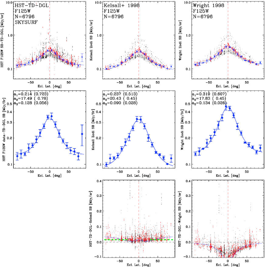
Figure 7: [(a) Top Left]: HST WFC3/IR sky-SB measurements in the F125W filter vs. Ecliptic Latitude after subtracting the best WFC3/IR Thermal Dark signal estimate for each exposure from § 3.3 and the Diffuse Galactic Light (DGL) signal from § 3.5. Black dots indicate all observations from Fig. 2, and red dots only those with Sun Angle SA=90$\pm$10^∘. The COBE/DIRBE data, to which the models were fit, were taken at a comparable SA-range. The blue points indicate the one-sided clipped medians of the SA=90$\pm$10^∘ points in each 10^∘ $b^{\rm Ecl}$-bin, and the blue line indicates the best $sech$-fit to these medians. [(b) Top Middle]: Kelsall et al. (1998) ZL model prediction for the same sky pointings and filters, observing day of the year, and Sun Angles as the HST data in (a) with their medians and best fit $sech$-model. [(c) Top Right]: As in (b), but for the Wright (1998) Zodiacal model prediction. [(d), (e), (f) Middle Row]: The clipped medians for each $b^{\rm Ecl}$-bin from panels (a), (b), (c) are reproduced for clarity, respectively, with their errors plus the best $sech$-fits and their coefficients. [(g) Bottom Middle]: Difference between each (HST–TD–DGL) data point from (a) and its Kelsall et al. (1998) ZL model prediction from (b), with the difference in their $sech$-fits (blue line). The green dashed line indicates the two-sided 1-sigma clipped median for SA=90$\pm$10^∘ and $|$$b^{\rm Ecl}$$|$$\gtrsim$30^∘ (Table 3). [(h) Bottom Right]: As in (g), but for the Wright (1998) Zodiacal model prediction from (c).

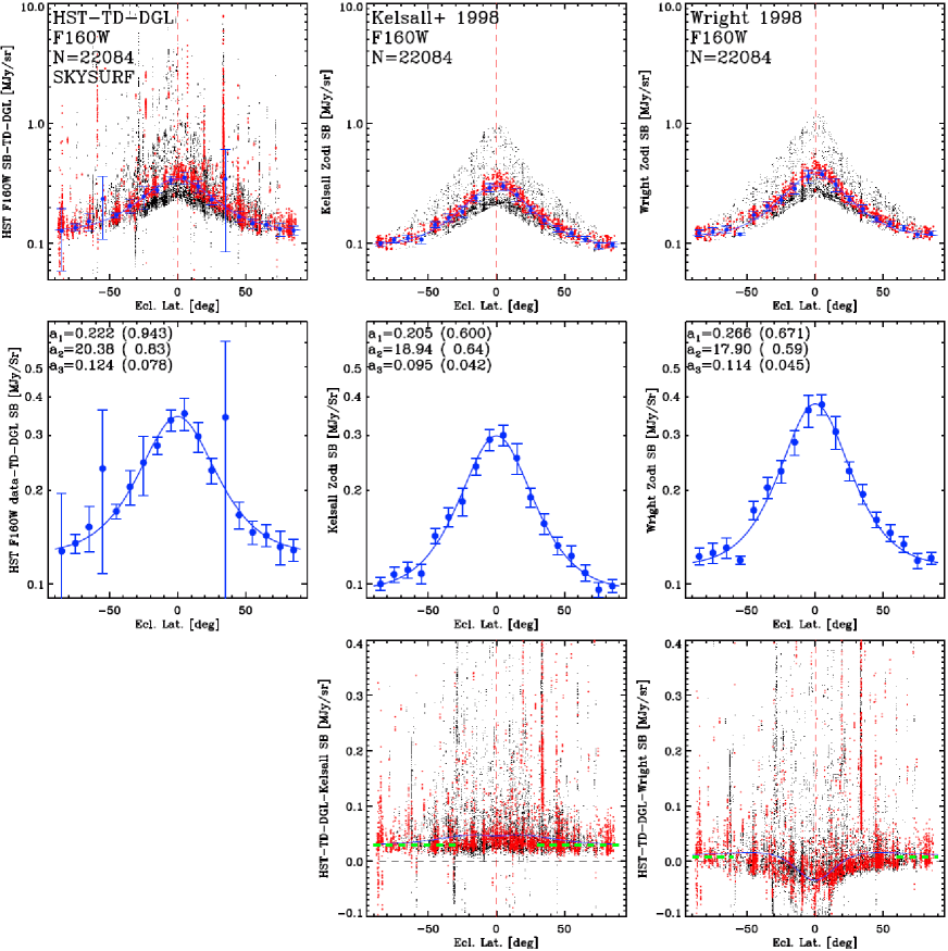
Figure 9: [(a) Top Left]: HST WFC3/IR sky-SB measurements in the F160W filter vs. Ecliptic Latitude after subtracting the best WFC3/IR Thermal Dark signal estimate for each exposure from § 3.3 and the Diffuse Galactic Light (DGL) signal from § 3.5. Black dots indicate all observations from Fig. 2, and red dots only those with Sun Angle SA=90$\pm$10^∘. The COBE/DIRBE data, to which the models were fit, were taken at a comparable SA-range. The blue points indicate the one-sided clipped medians of the SA=90$\pm$10^∘ points in each 10^∘ $b^{\rm Ecl}$-bin, and the blue line indicates the best $sech$-fit to these medians. [(b) Top Middle]: Kelsall et al. (1998) ZL model prediction for the same sky pointings and filters, observing day of the year, and Sun Angles as the HST data in (a) with their medians and best fit $sech$-model. [(c) Top Right]: As in (b), but for the Wright (1998) Zodiacal model prediction. [(d), (e), (f) Middle Row]: The clipped medians for each $b^{\rm Ecl}$-bin from panels (a), (b), (c) are reproduced for clarity, respectively, with their errors plus the best $sech$-fits and their coefficients. [(g) Bottom Middle]: Difference between each (HST–TD–DGL) data point from (a) and its Kelsall et al. (1998) ZL model prediction from (b), with the difference in their $sech$-fits (blue line). The green dashed line indicates the two-sided 1-sigma clipped median for SA=90$\pm$10^∘ and $|$$b^{\rm Ecl}$$|$$\gtrsim$30^∘ (Table 3). [(h) Bottom Right]: As in (g), but for the Wright (1998) Zodiacal model prediction from (c).

4 Discussion of SKYSURF’s First Results

In conclusion, the HST data–Kelsall et al. (1998) model allows for a diffuse light component of $\lesssim$29–40 nW m^-2 sr^-1 at 1.25–1.6 µm wavelength (Table 2). Given the relatively constant values of these HST–Kelsall offsets at most Ecliptic Latitudes (Fig. 7–9), these values may indicate a very dim, possibly spherical or ellipsoidal component of diffuse light in the net HST data that is not present in the Kelsall et al. (1998) model. This diffuse light level could be due to a number of causes: (a) a remaining HST orbital phase and temperature-dependent TD component, which may need to include a thermal Earthshine component; (b) a dim (nearly) spherical component missing in the Kelsall et al. (1998) Zodiacal Light model; (c) a spherical diffuse EBL component (Sano et al., 2020); or (d) some combination of these possibilities. The Wright (1998) model leaves little or no room for diffuse light after subtracting the Thermal Dark signal and DGL in Fig. 7–9 and Table 3. In this context, we compare our HST results with the following recent results by other groups:

(1) Matsuura et al. (2017) analyze CIBER rocket spectra, and find that the sky-SB of diffuse light at 1.4 µm wavelength is $\sim$42.7${}^{+11.7}_{-10.3}$ nW m^-2 sr^-1 compared to the Kelsall et al. (1998) model. After subtraction of a 1.4 µm iEBL+eEBL signal of $\sim$11.8 nW m^-2 sr^-1 (§ 3.4.3), this would correspond to a net diffuse light signal of $\sim$31 nW m^-2 sr^-1. They find no significant excess in diffuse light compared to the Wright (1998) model. They suggest that compared to the Kelsall et al. (1998) model their results may require “a new diffuse light component, such as an additional foreground or an excess EBL with a redder spectrum than that of the ZL.” Korngut et al. (2022) use subsequent CIBER spectra to estimate the Equivalent Width (EW) of the Ca triplet around 8542 Å, and suggest a simple modification to the Kelsall et al. (1998) model that adds a constant (spherical) component of 46$\pm$19 nW m^-2 sr^-1 to best fit their inferred Zodiacal level at 1.25 µm. The Korngut et al. (2022) CIBER experiment directly estimates the depth of the Ca triplet Fraunhofer lines in the Zodiacal spectrum, so it is plausible that much of this excess diffuse light is of Zodiacal origin. Within the errors, our 1.25–1.4 µm HST–Kelsall differences of $\lesssim$29–40 nW m^-2 sr^-1 are consistent with the diffuse light signal suggested by both Matsuura et al. (2017) and Korngut et al. (2022). Given that the lower envelopes of our 1.25–1.6 µm HST data–Kelsall model differences are rather constant at all higher Ecliptic Latitudes, it is thus possible that a dim, large, and largely spherical component may need to be added to the Kelsall et al. (1998) model with an amplitude of $\lesssim$29–40 nW m^-2 sr^-1 at 1.25–1.6 µm as seen from Low Earth Orbit.

Korngut et al. (2022) discuss that the heliocentric isotropic IPD distribution in the inner Solar System at 10–25 AU may be supplied by debris from long-period Oort Cloud Comets (OCC; Oort, 1950, see also, e.g., Nesvorný et al., 2010 and Poppe, 2016), and suggest that such a component may need to be added to the Kelsall et al. (1998) model with possibly a 5% amplitude. Our upper limits to the 1.25–1.6 µm sky-SB of $\lesssim$29–40 nW m^-2 sr^-1 in Table 2 and Fig. 10 suggest that any diffuse light is $\lesssim$10% of the Zodiacal sky-SB at these wavelengths. Hence, if most of this light were due to a missing component in the Kelsall et al. (1998) ZL model, such a component must be dim and extend to high Ecliptic latitudes. Future work is needed to add such a component to the Kelsall et al. (1998) model and match it to the SKYSURF observations. Revised models may need to include (a) collisional processes in the Solar System that can make the Zodiacal dust smaller over time, and (b) Solar radiation pressure that may drive these smaller dust particles further out into the Solar System, perhaps forming a tenuous ellipsoidal or more spherical cloud of dust around the Sun compared to the known Zodiacal IPD cloud.

The Kelsall et al. (1998) model includes IPD model uncertainties and lists possible changes that could improve the IPD modeling. Quoting their paper, one of their suggested improvements is: “7. Permit a variation of the albedo for the shorter wavelength bands to accommodate the clues in the observations that point to a variation with (Ecliptic) latitude, which may well result from the differences in the dust contributed by comets as compared to that coming from asteroids.” Table 2 of Kelsall et al. (1998) adopt an albedo at 1.25 µm wavelength for their Zodiacal components of $a$=0.204$\pm$0.0013. Recent thermal IR observations of TNOs imply geometric albedos of $\lesssim$20–30%, while some have albedos as large as $\sim$60% (e.g., Duffard et al., 2014; Kovalenko et al., 2017; Vilenius et al., 2012, 2014, 2018), possibly indicating a more icy surface for some TNOs. The four small satellites of Pluto have albedos ranging from 55%–85% (Weaver et al., 2016). While the nature of any OCC dust component at higher Ecliptic latitudes may be substantially different from that of TNOs and their collision or scattering products, these results suggest that albedos higher than the $a$$\simeq$0.2 value adopted by Kelsall et al. (1998) are possible. Future improvements of Zodiacal IPD models may therefore need to consider a different albedo distribution for any additional OCC dust component at higher Ecliptic latitudes, including albedos as appropriate for a larger fraction of dust particles with icy surfaces. For example, Sano et al. (2020) analyze DIRBE results, and find that the observed Sun Angle dependence of the mid-IR and near-IR background is consistent with an additional diffuse isotropic component with an amplitude of $\sim 5\%$ of the Kelsall et al. (1998) IPD cloud.

(2) Lauer et al. (2021) present 0.6 µm object counts from New Horizons images of 7 fields taken around Pluto’s distance, where the Zodiacal sky-SB is substantially lower than in LEO. They suggest a possible excess diffuse signal of unknown origin with an amplitude in the range (8.8–11.9)$\pm$4.6 nW m^-2 sr^-1 at 0.6 µm. These data are plotted with their two quoted error ranges as the blue points in Fig. 10 and Fig. 11. Lauer et al. (2022) add a single new NH field with lower DGL contribution, which has a similar 0.6 µm excess diffuse signal with a smaller error bar: 8.1 $\pm$ 1.9 nW m^-2 sr^-1(shown as the dark blue point in Fig 10-11). While their number of NH fields is limited, their images do provide a 0.6 µm diffuse light sky-SB estimate in the very dark sky environment at a distance of 43–51 AU from the Sun. Fig. 10 and 11 suggest their 0.6 µm upper value at 43–51 AU is about 8–10 nW m^-2 sr^-1 above the integrated and extrapolated discrete EBL of Driver et al. (2016) and Koushan et al. (2021), respectively, while our HST WFC3/IR 1.25–1.6 µm upper limits in Fig. 11 are about 29–40 nW m^-2 sr^-1 above the discrete EBL values at 1.25–1.6 µm.

The possible origin of 8–10 nW m^-2 sr^-1 of cosmological diffuse light remains an open question. For example, Conselice et al. (2016) and Lauer et al. (2021) suggested that some missing light could be caused by the galaxy counts rapidly steepening at V$\gtrsim$24 mag, because existing surveys are missing a substantial population of low-SB objects. Given the decreasing abundance of low-surface brightness objects with AB$\sim$24 and large sizes (e.g., Greene et al., 2022; Zaritsky et al., 2022), as well as recent limits on the abundance of low-surface brightness galaxies (e.g., Jones et al., 2018), it is hard to imagine that a factor of two or more in sky-SB comes from faint, undetected low-SB objects at V$\gtrsim$24 mag. Accounting of this diffuse light from even fainter galaxies becomes more difficult because they would have to be even more abundant to account for their corresponding faintness (e.g., Fig. 2 of SKYSURF-1). Further investigation of this possibility, as well as a more detailed analysis of the impact of surface brightness and confusion-based completeness on EBL estimations will be conducted with future SKYSURF analyses (e.g. Kramer et al. 2022, in preparation).

Any missing diffuse EBL would then also need to be present in our HST–Kelsall comparison, which allows for $\lesssim$29–40 nW m^-2 sr^-1 of diffuse light at 1.25–1.6 µm. If for instance $\lesssim$10 nW m^-2 sr^-1 of our HST–Kelsall difference were due to truly diffuse EBL of cosmological origin (i.e., very faint, low-SB objects), then the Kelsall et al. (1998) model would only need $\sim$20 nW m^-2 sr^-1 of additional uniform Zodiacal component. However, our HST data–Wright model comparison does not require this, and, in fact, leaves little or no room for any additional diffuse light components, neither an unrecognized HST Thermal Dark signal component, nor an additional Zodiacal component, nor a diffuse EBL component.

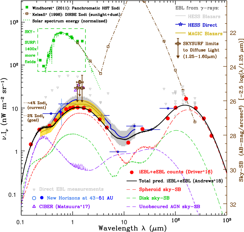
Figure 10: Summary of astrophysical foreground and background energy relevant to SKYSURF, along with the first SKYSURF measurements at $1.25$, $1.37$, and $1.53$ microns. The left scale indicates the total energy $\nu$.$I_{\nu}$ in nW m^-2 sr^-1, and the right scale the corresponding sky-SB in AB-mag arcsec^-2 at 1.25 µm (which can be scaled to other wavelengths as indicated). The discrete measurements of D16 from integrated and extrapolated galaxy counts (iEBL+eEBL) (red-filled circles) and other published data are shown. Grey triangles indicate the total EBL measurements (Puget et al., 1996; Fixsen et al., 1998; Dwek & Arendt, 1998; Hauser et al., 1998; Lagache et al., 1999; Finkbeiner et al., 2000; Dole et al., 2006; Bernstein et al., 2002; Bernstein, 2007; Cambrésy et al., 2001; Matsumoto et al., 2005; Matsuura et al., 2011; Matsumoto et al., 2011; Tsumura et al., 2013; Sano et al., 2020). Also shown are more recent results from the CIBER experiment (purple triangles; Matsuura et al. 2017), Pioneer (light blue points without errors; Matsumoto et al. 2018), and New Horizons (medium and dark-blue points with errors; Lauer et al. 2021 and Lauer et al. 2022, which is offset for clarity) that aim to more accurately subtract the Zodiacal foreground. All of these measurements require accurate modeling of foreground DGL, and, except for Pioneer and New Horizons points, ZL. For a more direct comparison with SKYSURF diffuse-light limits, the iEBL level (taken from the respective references) has been subtracted from the CIBER and New Horizons points. Green squares are panchromatic HST sky-SB measurements compared to the Solar spectrum. Brown squares indicate the COBE/DIRBE data and the Zodiacal dust model of Kelsall et al. (1998). The grey and orange wedges and blue stars are $\gamma$-ray Blazar EBL constraints from the MAGIC and HESS TeV experiments (MAGIC Collaboration et al., 2008; H. E. S. S. Collaboration et al., 2013). The black line is the sum of the Andrews et al. (2018) EBL models for star-formation in spheroids (red), disks (green), and unobscured AGN (purple). The currently achieved calibration+zeropoint accuracy in the 1.25–1.6 µm HST sky-SB estimates is $\sim$4% of the Zodiacal sky-SB (Windhorst et al., 2022), as indicated. SKYSURF’s goal is a $\lesssim$2%-accurate sky-SB model across the sky at 0.2-1.6 µm wavelengths to address the discrepancy between the total EBL and the discrete iEBL+eEBL. The brown points are the SKYSURF diffuse light limits, which implicitly subtract discrete iEBL, identified in Table 1. These limits are lower than previous analyses, but still leave room for an isotropic diffuse light component, whether in the Solar System or at cosmological distances.

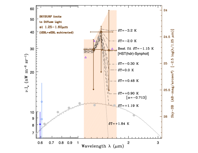
Figure 11: SKYSURF on the level of diffuse light compared with limits on diffuse light. As in Fig. 10, purple triangles and blue open and filled circles are from Matsuura et al. (2017), Lauer et al. (2021), and Lauer et al. (2022) respectively. Also shown for context are iEBL estimates from Koushan et al. (2021) as the grey points, and the Driver et al. (2016) model fit to those measurements as the grey line. The large open orange circles with their error ranges are the SKYSURF diffuse light upper limits in the WFC3/IR filters F125W, F140W, and F160W, as discussed in § 3.1–3.6, Figs. 5–9 and Table 1–3, from which the iEBL+eEBL has already been subtracted. The shaded orange wedge indicates our diffuse light limits given the current best knowledge of the HST temperature range and its resulting WFC3/IR Thermal Dark signal, and the subtracted discrete iEBL+eEBL signal (§ 3). The $synphot$ HST component temperature predictions can vary by $\Delta$T$\simeq$$\pm$2 K from those in the HST engineering data and FITS headers. The best $\chi^{2}$ -fit occurs for an average ($pysynphot$–HST-header) difference of $\Delta$T=–1.15 K. The $\Delta$T value that is most consistent with the 1–2 µm Kelsall slope of the Zodiacal spectrum ($\alpha$=0.713; see § 3.4) is also indicated, and occurs for (HST-header–$synphot$) temperature difference of $\Delta$T=+0.90 K. Therefore, while our limits to the F125W and F140W diffuse light are a factor $\sim$3 above the best available discrete EBL counts of Koushan et al. (2021), any diffuse signal in the F160W filter could be fainter still, as indicated by the orange wedge. The upper limits of the orange wedge correspond to the limits derived from the SA90 method. Details are given in § 3–4. At 1.25 and 1.4 microns, the detection of diffuse light is not very dependent on the assumed thermal dark signal. While our fiducial F160W results are consistent with the F125W and F140W limits, the F160W limit depends much more strongly on the assumed thermal dark signal.

In conclusion, the darkest $\sim$1% of our 34,000 HST WFC3/IR 1.25–1.6 µm images closely follow the shape of the Kelsall et al. (1998) model, and suggest that the Kelsall et al. (1998) model may need an additional (nearly spherical) component of $\lesssim$29–40 nW m^-2 sr^-1, while HST shows no such excess over the Wright (1998) model. A possible explanation is that the Kelsall model may be missing $\lesssim$29–40 nW m^-2 sr^-1 of high albedo OCC dust as seen from 1 AU, which Wright (1998) included by default, because of his assumed strong no-Zodiacal condition at 25 µm wavelength.

Through the “Sungrazer” project (Sekanina & Kracht, 2013) , orbiting Solar observatories like SOHO and STEREO have found thousands of comets since 1995 that are getting in close proximity of the Sun. Silsbee & Tremaine (2016) have modeled the nearly isotropic comet population that are expected to show up in very large numbers — also at larger distances from the Sun — with the Rubin Telescope . Hence, updated Zodiacal IPD models may be able to include a more spherical component from such cometary dust left behind in the inner solar system.

HST studies of KBO’s at $\sim$10–100 AU show remarkably blue colors in the WFC3/IR medium-band filters F139M–F153M (e.g., Fraser & Brown, 2012; Fraser et al., 2015), which have similar central wavelengths but are narrower than our F140W and F160W filters. While it remains to be seen that OCC dust in the outer Solar System has similar blue near-IR colors and high reflectance, scattering models of icy particles (including amorphous and crystalline H₂O ice) do suggest that high albedos with a near-IR wavelength dependence are possible. ZL model refinements may need to include such considerations in more detail to better match the LFS envelopes of the HST data at all Ecliptic latitudes. We consider this in future papers when the full panchromatic SKYSURF database has been processed including all the UV–optical and remaining near-IR filters. Once Zodiacal Light models have been updated to fully match the panchromatic SKYSURF data, this may result in firmer limits to, or estimates of, the amount of diffuse light that can come from beyond our Solar System, including diffuse EBL.

5 Summary and Conclusions

In this paper, we present the first results from the Hubble Space Telescope Archival project “SKYSURF”, first outlined in (SKYSURF-1). Sky surface brightness measurements conducted on HST data are confirmed to be stable and precise, in line with the $\sim 2-4\%$ errors estimated in SKYSURF-1. By comparing measured HST sky-surface brightness measurements with predictions describing Zodiacal and Galactic foregrounds, we place competitive limits on the presence of an isotropic diffuse light component, either within the Solar System or at cosmological distances.

$\bullet$ (1) Without having reprocessed the entire HST imaging Archive for SKYSURF as yet, we illustrate our methods and first results from 34,412 images in the HST Wide Field Camera 3 IR filters F125W, F140W, and F160W. Compared to the COBE/DIRBE 1.25 µm and K-band Zodiacal sky-SB predictions of Kelsall et al. (1998), our darkest WFC3 F125W, F140W, and F160W sky-SB measurements appear to be on average $\sim$15–55% higher (or $\sim$0.0145$\pm$0.008, 0.025$\pm$0.009, and 0.048$\pm$0.009 MJy/sr, respectively) than the Kelsall et al. (1998) model predictions. With both taken at face value, this places an upper limit of $\lesssim$29–40 nW m^-2 sr^-1 on any 1.25–1.6 µm diffuse light in excess of the Kelsall et al. (1998) ZL model components.

$\bullet$ (2) The largest uncertainty in our darkest HST WFC3/IR sky-SB measurements comes from the WFC3/IR Thermal Dark signal subtraction at 1.6 µm. From multi-wavelength WFC3/IR images, we assess and subtract the WFC3/IR Thermal Dark signal for a range of HST orbital temperatures (–3$\lesssim$$\Delta$T$\lesssim$3 K). In the F160W filter, the Thermal Dark signal may be as large as the value of our upper limit to any remaining diffuse light if HST were to run hotter than nominal by $\gtrsim$+2 K, leaving in that case little room for a significant diffuse light component. However, for the best-fit $\Delta$T=–1.15 K below the HST reference temperature, the nominal F160W Thermal Dark signal is $\sim$0.077 e^-/pix/sec (or $\sim$0.031 MJy/sr), resulting in a fairly consistent net diffuse light signal in all three HST filters less than 29–40 nW m^-2 sr^-1 over the Kelsall et al. (1998) model predictions that were made for the same sky pointings and filters, observing day of the year, and Sun Angle.

$\bullet$ (3) Compared to the Wright (1998) ZL model, HST appears to detect no significant 1.25–1.6 µm diffuse light within the current uncertainties. The lower envelope of the HST data–Wright model values suggests no remaining signal in the F125W and F140W filters or perhaps a slightly negative one. In the F160W filter, the HST data–Wright model values suggest a remaining diffuse signal of at most $\sim$0.0077 MJy/sr (15 nW m^-2 sr^-1). Hence, if the Wright (1998) model best represents the ZL, this model would leave little or no room for additional diffuse light components.

$\bullet$ In conclusion, given our Lowest Fitted Sky-SB measurements in the HST WFC3/IR F125W, F140W, and F160W filters, an update of the Kelsall et al. (1998) ZL model may be needed to better understand and constrain any additional diffuse light components that may come from the outer Solar System. Once those are modeled in more detail and over a wider range of wavelengths, better constraints may also be obtained on any remaining diffuse light component, including diffuse EBL. This will be addressed in future SKYSURF papers.

Appendix A Thermal Behavior of HST

Temperatures of the HST components are monitored through various thermal sensors throughout the telescope and WFC3. The HST component temperatures utilized as reference temperatures in §3.4.1 were taken from tables in https://www.stsci.edu/hst/instrumentation/reference-data-for-calibration-and-tools/synphot-throughput-tables, and are summarized below in Table 4. Here, we also reproduce some representative values of relevant telescope components directly from the STScI HST telescope group (private communication), which are not all directly available through the HST image FITS headers, $ima$- or or jit-files. The $T_{\rm ref}$ values are generally consistent with temperatures measured by sensors on the telescope to a few degrees C.

Table 4: $T_{\rm ref}$ of HST optical components

Component    $|$	Temperature (∘C)
Primary Mirror	15.15
Mirror Pads	15.15
Secondary Mirror	17.15
Pick of Mirror	14.75
IR Chanel Select Mechanism	0.15
Fold Mirror	0.15
WFC3IR Mirror 1	0.15
WFC3IR Mirror 2	0.15
WFC3IR Refractive Corrector Plate	-35.85
WFC3IR Filter	-35.85

HST’s thermal variations across each orbit will matter the most for WFC3/IR, as the IR detector is most sensitive for measurable thermal variations at wavelengths $\lambda$$\gtrsim$1.4 µm. (To avoid excessive Thermal Dark signal in the H-band, the WFC3/IR detector was therefore designed to cut-out all wavelengths $\lambda$$\gtrsim$1.73 µm, so that the WFC3/IR F160W filter therefore is really a “short H-band” filter with $\lambda_{eff}$ $\simeq$1.53 µm). During 2020, typical temperatures measured were (working backwards from the IR detector; all in units of degrees C): IR Detector = –127.8 C; IR Shield = –100.2 C (the black inner housing surrounding the detector); Outer IR Detector Housing = –48.75 C; Housing of the IR Filter Select Mechanism (FSM) = –55 C; Refractive Corrector Plate (RCP) = –33.62 C; and the WFC3/IR Cold Enclosure (CE) = –33.6 C. These are the temperatures of the components seen by the WFC3/IR detector directly, and can vary by a couple degrees C.

When the (aluminum) Blank is selected for Dark Current measurements in the WFC3/IR FSM, it blocks the detector’s view of the WFC3/IR RCP, so only indirect illumination from the CE is possible. This Blank has higher emissivity than the WFC3/IR filters, so a measured Dark Current frame looking at the aluminum Blank will contain additional Thermal Dark signal and have a somewhat higher amplitude than the dark frame that is applicable to most filters. WFC3 does not have a temperature sensor on the FSM filters and the Blank, but their temperatures are likely somewhere between the FSM Housing at –55 C and the RCP at –33.6 C. All of this thermal emission comes from the entire passband of the IR detector (i.e., 0.6–1.73 µm). Therefore, when a WFC3/IR dark frame is taken to form a Dark Current calibration file to be subtracted in the WFC3 pipeline, only the thermal sources between the Blank and the detector listed above plus the actual detector generated Dark Current are measured.

The WFC3/IR filters have very high transmission and will also transmit some Thermal Dark signal from the camera and the telescope, which are at different temperatures but come from much smaller solid angles. The Dark Current calibration required thus does depend upon which filter was used for the science observation. With a WFC3/IR filter in place, we see the RCP, four mirrors within the WFC3 optical bench cold-enclosure, and the WFC3 Pick-Off Mirror (POM) in the OTA Hub Area. Temperatures of these are somewhat less precisely known due to the lack of close temperature sensors. The POM picks up more thermal radiation from the Earth during occultation, which subsequently cools off when the observations start during the next darker part of an orbit. The four mirrors inside the WFC3 enclosure are at temperatures of about 0–4 C. They are all silver coated and thus have fairly low emissivity within the IR filter passbands, slightly lower than that of gold.

The WFC3 optical bench and all of its associated baffles provide an environment kept colder than +4 C, but with higher emissivity. The cold mask at the location of the RCP has about the same temperature as the RCP and should block all direct views of these high emissivity surfaces, i.e., the WFC3 detector only has a direct view of HST’s mirrors. The WFC3 POM consists of a MgF₂ flat substrate overcoated with aluminum to ensure excellent near-UV performance. Its temperature is less certain, because of the lack of nearby temperature sensors, but the arm to which it is attached is at +12.5 C, and the “snout” leading into the WFC3 optical bench is at +7.9$\pm$0.7 C. The POM sees the illuminated Earth during most orbits and therefore fluctuates in temperature. It is unknown by exactly how much, as this depends on the Earth scenes transiting during bright time, but it is likely that the POM varies between 10–15 degrees C. The OTA primary and secondary mirrors, and their associated baffles are also typically at 10–17 C, although the baffles will not matter much for Thermal Dark signal estimates.

All these surfaces with their measured or estimated temperatures and approximate geometries have been modeled using simple black-body approximations in the $pysynphot$ tool and the appropriate emissivities and solid angles as seen from the detector. Given the incomplete knowledge of exact temperatures and their ranges, as well as of all the precise geometries inside WFC3 and HST, these $pysynphot$ predictions of the WFC3/IR Thermal Dark signal will have their limitations. Hence, in § 3.3 we present the best available $pysynphot$ estimates of the WFC3/IR Thermal Dark signal based on these average temperatures in order to analyze our WFC3/IR sky-SB measurements, including a plausible temperature range of HST’s main components as modeled in $pysynphot$. We refer to Carleton et al. (2022b, in preparation) for a detailed analysis of the most likely Thermal Dark signal for each WFC3/IR exposure in the SKYSURF database.

Appendix B Acronyms Used in SKYSURF

Acronym	Explanation
AB-mag	–2.5 log (Object-Flux / Zeropoint-Flux)
ACS	Advanced Camera for Surveys
AGN	Active Galactic Nucleus
APT	Astronomers Proposal Tool
ASU	Arizona State University
AWS	Amazon Web Services
CCD	Charged Coupled Device
CDM	Cold Dark Matter
CERES	Clouds and the Earth’s Radiant Energy System
CIB	Cosmic Infrared Background
COB	Cosmic Optical Background
COBE	Cosmic Background Explorer
COS	HST’s Cosmic Origins Spectrograph
CR	Cosmic Ray
CTE	Charge Transfer Efficiency
CV	Cosmic Variance
CVZ	Continuous Viewing Zone
DC	(Electronic) Dark Current
DGL	Diffuse Galactic Light
DIRBE	Diffuse Infra-Red Background Experiment
EBL	Extragalactic Background Light
dEBL	diffuse Extragalactic Background Light
eEBL	extrapolated Extragalactic Background Light
iEBL	integrated Extragalactic Background Light
ERS	(HST WFC3) Early Release Science program
FOC	HST’s Faint Object Camera
FOS	HST’s Faint Object Spectrograph
FOV	Field of View
FWHM	Full-Width Half-Maximum
GDC	Geometrical Distortion Corrections
GOODS	Great Orbiting Observatories Deep Survey
$H_{AB}$	H-band (1.6 µm) AB-mag
HDF	Hubble Deep Field
HLA	Hubble Legacy Archive
HLC	Hubble Legacy Catalog
HST	Hubble Space Telescope
HUDF	Hubble UltraDeep Field
HWHM	Half Width Half Maximum (=0.5$\times$FWHM)
ICL	Intra-Cluster Light
IEF	Illuminated Earth Fraction

ACRONYMS USED IN SKYSURF (continued)

Acronym	Explanation
IGL	Intra-Group Light
IPD	InterPlanetary Dust
IRAF	Image Reduction and Analysis Facility
ISM	Interstellar Medium
$J_{AB}$	J-band (1.25 µm) AB-mag
Jy	Jansky or Flux Density unit (=10-26$W\ m^{-2}\ Hz^{-1}$)
KBOs	Kuiper Belt Objects
LA	Earth’s Limb Angle
LEO	Low Earth Orbit
LES	Lowest Estimated Sky-SB
LFS	Lowest Fitted Sky-SB
MA	Moon Angle
MAST	Mikulski Archive for Space Telescopes
NED	NASA Extragalactic Database
NEP	North Ecliptic Pole
NICMOS	Near-Infrared Camera and Multi-Object Spectrograph
OCC	Oort Cloud Comets
OTA	Optical Telescope Assembly
PAM	Pixel Area Map
PSF	Point Spread Function
QSOs	Quasi Stellar Objects
RA	HST Roll Angle
R.A.	Right Ascension
RC3	Third Reference Catalog of Bright Galaxies
SAA	South Atlantic Anomaly
SA	Sun Angle
SB	Surface Brightness
SDSS	Sloan Digital Sky Survey
SED	Spectral Energy Distribution
SEP	South Ecliptic Pole
SFR	Star-Formation Rate
SF	Star-Forming
SM	Servicing Mission
STIS	Space Telescope Imaging Spectrograph
STScI	Space Telescope Science Institute
TD	Thermal Dark signal
TNOs	Trans-Neptunian Objects
UVIS	WFC3 UV–Visual channel
UV	Ultraviolet ($\sim$0.1–0.3 µm)
WFC3	HST’s Wide Field Camera 3
WFPC2	HST’s Wide Field Planetary Camera 2
WF/PC	HST’s Wide Field/Planetary Camera
ZL	Zodiacal Light

References

- Aldering (2001) Aldering, G. 2001, LBNL report, LBNL-51157, 1
- Andrews et al. (2018) Andrews, S. K., Driver, S. P., Davies, L. J. M., Lagos, C. d. P., & Robotham, A. S. G. 2018, MNRAS, 474, 898
- Arendt (2014) Arendt, R. G. 2014, AJ, 148, 135
- Arendt et al. (2016) Arendt, R. G., Kashlinsky, A., Moseley, S. H., & Mather, J. 2016, ApJ, 824, 26
- Arendt et al. (1998) Arendt, R. G., Odegard, N., Weiland, J. L., et al. 1998, ApJ, 508, 74
- Arvesen et al. (1969) Arvesen, J. C., Griffin, Roy N., J., & Pearson, B. Douglas, J. 1969, Appl. Opt., 8, 2215
- Ashcraft et al. (2018) Ashcraft, T. A., Windhorst, R. A., Jansen, R. A., et al. 2018, PASP, 130, 064102
- Astropy Collaboration et al. (2013) Astropy Collaboration, Robitaille, T. P., Tollerud, E. J., et al. 2013, A&A, 558, A33
- Astropy Collaboration et al. (2018) Astropy Collaboration, Price-Whelan, A. M., Sipőcz, B. M., et al. 2018, AJ, 156, 123
- Bernstein et al. (1995) Bernstein, G. M., Nichol, R. C., Tyson, J. A., Ulmer, M. P., & Wittman, D. 1995, AJ, 110, 1507
- Bernstein (2007) Bernstein, R. A. 2007, ApJ, 666, 663
- Bernstein et al. (2002) Bernstein, R. A., Freedman, W. L., & Madore, B. F. 2002, ApJ, 571, 56
- Bertin & Arnouts (1996) Bertin, E., & Arnouts, S. 1996, A&AS, 117, 393
- Borlaff et al. (2019) Borlaff, A., Trujillo, I., Román, J., et al. 2019, A&A, 621, A133
- Bradley et al. (2020) Bradley, L., Sipőcz, B., Robitaille, T., et al. 2020, astropy/photutils: 1.0.0, v.1.0.0, Zenodo, doi:10.5281/zenodo.4044744
- Brandt & Draine (2012) Brandt, T. D., & Draine, B. T. 2012, ApJ, 744, 129
- Cambrésy et al. (2001) Cambrésy, L., Reach, W. T., Beichman, C. A., & Jarrett, T. H. 2001, ApJ, 555, 563
- Cheng et al. (2021) Cheng, Y.-T., Arai, T., Bangale, P., et al. 2021, ApJ, 919, 69
- Conselice et al. (2016) Conselice, C. J., Wilkinson, A., Duncan, K., & Mortlock, A. 2016, ApJ, 830, 83
- Cooray (2016) Cooray, A. 2016, Royal Society Open Science, 3, 150555
- Cooray et al. (2004) Cooray, A., Bock, J. J., Keatin, B., Lange, A. E., & Matsumoto, T. 2004, ApJ, 606, 611
- Dalcanton et al. (1997) Dalcanton, J. J., Spergel, D. N., Gunn, J. E., Schmidt, M., & Schneider, D. P. 1997, AJ, 114, 635
- de Grijs et al. (1997) de Grijs, R., Peletier, R. F., & van der Kruit, P. C. 1997, A&A, 327, 966
- Dole et al. (2006) Dole, H., Lagache, G., Puget, J. L., et al. 2006, A&A, 451, 417
- Domínguez et al. (2011) Domínguez, A., Primack, J. R., Rosario, D. J., et al. 2011, MNRAS, 410, 2556
- Dressel (2021) Dressel, L. 2021, “Wide Field Camera 3 Instrument Handbook”, Version 13.0, (Baltimore: STScI), ,
- Driver et al. (1995) Driver, S. P., Windhorst, R. A., Ostrander, E. J., et al. 1995, ApJ, 449, L23
- Driver et al. (2011) Driver, S. P., Hill, D. T., Kelvin, L. S., et al. 2011, MNRAS, 413, 971
- Driver et al. (2016) Driver, S. P., Andrews, S. K., Davies, L. J., et al. 2016, ApJ, 827, 108
- Duffard et al. (2014) Duffard, R., Pinilla-Alonso, N., Santos-Sanz, P., et al. 2014, A&A, 564, A92
- Dwek & Arendt (1998) Dwek, E., & Arendt, R. G. 1998, ApJ, 508, L9
- Dwek & Krennrich (2013) Dwek, E., & Krennrich, F. 2013, Astroparticle Physics, 43, 112
- Finkbeiner et al. (2000) Finkbeiner, D. P., Davis, M., & Schlegel, D. J. 2000, ApJ, 544, 81
- Finke et al. (2010) Finke, J. D., Razzaque, S., & Dermer, C. D. 2010, ApJ, 712, 238
- Fixsen et al. (1998) Fixsen, D. J., Dwek, E., Mather, J. C., Bennett, C. L., & Shafer, R. A. 1998, ApJ, 508, 123
- Fraser & Brown (2012) Fraser, W. C., & Brown, M. E. 2012, ApJ, 749, 33
- Fraser et al. (2015) Fraser, W. C., Brown, M. E., & Glass, F. 2015, ApJ, 804, 31
- Fraser et al. (2014) Fraser, W. C., Brown, M. E., Morbidelli, A., Parker, A., & Batygin, K. 2014, ApJ, 782, 100
- Fuentes et al. (2009) Fuentes, C. I., George, M. R., & Holman, M. J. 2009, ApJ, 696, 91
- Gorjian et al. (2000) Gorjian, V., Wright, E. L., & Chary, R. R. 2000, ApJ, 536, 550
- Greene et al. (2022) Greene, J. E., Greco, J. P., Goulding, A. D., et al. 2022, ApJ, 933, 150
- Guhathakurta & Tyson (1989) Guhathakurta, P., & Tyson, J. A. 1989, ApJ, 346, 773
- H. E. S. S. Collaboration et al. (2013) H. E. S. S. Collaboration, Abramowski, A., Acero, F., et al. 2013, A&A, 550, A4
- Hauser & Dwek (2001) Hauser, M. G., & Dwek, E. 2001, ARA&A, 39, 249
- Hauser et al. (1998) Hauser, M. G., Arendt, R. G., Kelsall, T., et al. 1998, ApJ, 508, 25
- Helou & Walker (1985) Helou, G., & Walker, D. W. 1985, IRAS small scale structure catalog
- Impey et al. (1988) Impey, C., Bothun, G., & Malin, D. 1988, ApJ, 330, 634
- Jones et al. (2018) Jones, M. G., Papastergis, E., Pandya, V., et al. 2018, A&A, 614, A21
- Jorgensen et al. (2021) Jorgensen, J. L., Benn, M., Connerney, J. E. P., et al. 2021, Journal of Geophysical Research (Planets), 126, e06509
- Kashlinsky (2005) Kashlinsky, A. 2005, Phys. Rep., 409, 361
- Kashlinsky et al. (2004) Kashlinsky, A., Arendt, R., Gardner, J. P., Mather, J. C., & Moseley, S. H. 2004, ApJ, 608, 1
- Kelsall et al. (1998) Kelsall, T., Weiland, J. L., Franz, B. A., et al. 1998, ApJ, 508, 44
- Kenyon & Bromley (2004) Kenyon, S. J., & Bromley, B. C. 2004, AJ, 128, 1916
- Kenyon & Bromley (2020) —. 2020, PSJ, 1, 40
- Kenyon & Luu (1999) Kenyon, S. J., & Luu, J. X. 1999, AJ, 118, 1101
- Kenyon & Windhorst (2001) Kenyon, S. J., & Windhorst, R. A. 2001, ApJ, 547, L69
- Khaire & Srianand (2015) Khaire, V., & Srianand, R. 2015, ApJ, 805, 33
- Korngut et al. (2022) Korngut, P. M., Kim, M. G., Arai, T., et al. 2022, ApJ, 926, 133
- Koushan et al. (2021) Koushan, S., Driver, S. P., Bellstedt, S., et al. 2021, MNRAS, 503, 2033
- Kovalenko et al. (2017) Kovalenko, I. D., Doressoundiram, A., Lellouch, E., et al. 2017, A&A, 608, A19
- Lagache et al. (1999) Lagache, G., Abergel, A., Boulanger, F., Désert, F. X., & Puget, J. L. 1999, A&A, 344, 322
- Lagache et al. (2005) Lagache, G., Puget, J.-L., & Dole, H. 2005, ARA&A, 43, 727
- Landsman (1993) Landsman, W. B. 1993, in Astronomical Society of the Pacific Conference Series, Vol. 52, Astronomical Data Analysis Software and Systems II, ed. R. J. Hanisch, R. J. V. Brissenden, & J. Barnes, 246
- Lauer et al. (2021) Lauer, T. R., Postman, M., Weaver, H. A., et al. 2021, ApJ, 906, 77
- Lauer et al. (2022) Lauer, T. R., Postman, M., Spencer, J. R., et al. 2022, ApJ, 927, L8
- Leinert et al. (1998) Leinert, C., Bowyer, S., Haikala, L. K., et al. 1998, A&AS, 127, 1
- Leisman et al. (2017) Leisman, L., Haynes, M. P., Janowiecki, S., et al. 2017, ApJ, 842, 133
- Madau & Dickinson (2014) Madau, P., & Dickinson, M. 2014, ARA&A, 52, 415
- MAGIC Collaboration et al. (2008) MAGIC Collaboration, Albert, J., Aliu, E., et al. 2008, Science, 320, 1752
- Matsumoto et al. (2018) Matsumoto, T., Tsumura, K., Matsuoka, Y., & Pyo, J. 2018, AJ, 156, 86
- Matsumoto et al. (2005) Matsumoto, T., Matsuura, S., Murakami, H., et al. 2005, ApJ, 626, 31
- Matsumoto et al. (2011) Matsumoto, T., Seo, H. J., Jeong, W. S., et al. 2011, ApJ, 742, 124
- Matsuura et al. (2011) Matsuura, S., Shirahata, M., Kawada, M., et al. 2011, ApJ, 737, 2
- Matsuura et al. (2017) Matsuura, S., Arai, T., Bock, J. J., et al. 2017, ApJ, 839, 7
- McVittie & Wyatt (1959) McVittie, G. C., & Wyatt, S. P. 1959, ApJ, 130, 1
- Metcalfe et al. (1995) Metcalfe, N., Shanks, T., Fong, R., & Roche, N. 1995, MNRAS, 273, 257
- Mihos et al. (2005) Mihos, J. C., Harding, P., Feldmeier, J., & Morrison, H. 2005, ApJ, 631, L41
- Nesvorný et al. (2010) Nesvorný, D., Jenniskens, P., Levison, H. F., et al. 2010, ApJ, 713, 816
- Odewahn et al. (1996) Odewahn, S. C., Windhorst, R. A., Driver, S. P., & Keel, W. C. 1996, ApJ, 472, L13
- Oke & Gunn (1983) Oke, J. B., & Gunn, J. E. 1983, ApJ, 266, 713
- Onishi et al. (2018) Onishi, Y., Sano, K., Matsuura, S., et al. 2018, PASJ, 70, 76
- Oort (1950) Oort, J. H. 1950, Bull. Astron. Inst. Netherlands, 11, 91
- Partridge & Peebles (1967a) Partridge, R. B., & Peebles, P. J. E. 1967a, ApJ, 147, 868
- Partridge & Peebles (1967b) —. 1967b, ApJ, 148, 377
- Planck Collaboration et al. (2016) Planck Collaboration, Ade, P. A. R., Aghanim, N., et al. 2016, A&A, 594, A13
- Poppe (2016) Poppe, A. R. 2016, Icarus, 264, 369
- Puget et al. (1996) Puget, J. L., Abergel, A., Bernard, J. P., et al. 1996, A&A, 308, L5
- Reach et al. (1997) Reach, W. T., Franz, B. A., & Weiland, J. L. 1997, Icarus, 127, 461
- Robotham et al. (2018) Robotham, A. S. G., Davies, L. J. M., Driver, S. P., et al. 2018, MNRAS, 476, 3137
- Robotham et al. (2017) Robotham, A. S. G., Taranu, D. S., Tobar, R., Moffett, A., & Driver, S. P. 2017, MNRAS, 466, 1513
- Saldana-Lopez et al. (2021) Saldana-Lopez, A., Domínguez, A., Pérez-González, P. G., et al. 2021, MNRAS, 507, 5144
- Sano & Matsuura (2017) Sano, K., & Matsuura, S. 2017, ApJ, 849, 31
- Sano et al. (2020) Sano, K., Matsuura, S., Yomo, K., & Takahashi, A. 2020, ApJ, 901, 112
- Santos et al. (2002) Santos, M. R., Bromm, V., & Kamionkowski, M. 2002, MNRAS, 336, 1082
- Schlegel et al. (1998) Schlegel, D. J., Finkbeiner, D. P., & Davis, M. 1998, ApJ, 500, 525
- Sekanina & Kracht (2013) Sekanina, Z., & Kracht, R. 2013, ApJ, 778, 24
- Shankman et al. (2013) Shankman, C., Gladman, B. J., Kaib, N., Kavelaars, J. J., & Petit, J. M. 2013, ApJ, 764, L2
- Silsbee & Tremaine (2016) Silsbee, K., & Tremaine, S. 2016, AJ, 152, 103
- Singer et al. (2019) Singer, K. N., McKinnon, W. B., Gladman, B., et al. 2019, Science, 363, 955
- Soifer et al. (1984) Soifer, B. T., Rowan-Robinson, M., Houck, J. R., et al. 1984, ApJ, 278, L71
- Szomoru & Guhathakurta (1998) Szomoru, A., & Guhathakurta, P. 1998, ApJ, 494, L93
- Tsumura et al. (2013) Tsumura, K., Matsumoto, T., Matsuura, S., et al. 2013, PASJ, 65, 119
- Tyson (1988) Tyson, J. A. 1988, AJ, 96, 1
- van der Kruit (1988) van der Kruit, P. C. 1988, A&A, 192, 117
- van Dokkum et al. (2015) van Dokkum, P. G., Abraham, R., Merritt, A., et al. 2015, ApJ, 798, L45
- Vilenius et al. (2012) Vilenius, E., Kiss, C., Mommert, M., et al. 2012, A&A, 541, A94
- Vilenius et al. (2014) Vilenius, E., Kiss, C., Müller, T., et al. 2014, A&A, 564, A35
- Vilenius et al. (2018) Vilenius, E., Stansberry, J., Müller, T., et al. 2018, A&A, 618, A136
- Weaver et al. (2016) Weaver, H. A., Buie, M. W., Buratti, B. J., et al. 2016, Science, 351, aae0030
- Windhorst et al. (2011) Windhorst, R. A., Cohen, S. H., Hathi, N. P., et al. 2011, ApJS, 193, 27
- Windhorst et al. (2022) Windhorst, R. A., Carleton, T., O’Brien, R., et al. 2022, arXiv e-prints, arXiv:2205.06214
- Wright (1998) Wright, E. L. 1998, ApJ, 496, 1
- Wright (2001) —. 2001, ApJ, 553, 538
- Wright et al. (2010) Wright, E. L., Eisenhardt, P. R. M., Mainzer, A. K., et al. 2010, AJ, 140, 1868
- Zaritsky et al. (2022) Zaritsky, D., Donnerstein, R., Karunakaran, A., et al. 2022, ApJS, 261, 11
- Zubko et al. (2004) Zubko, V., Dwek, E., & Arendt, R. G. 2004, ApJS, 152, 211