Effects of Lorentz violation in the Higgs sector of the Minimal Standard Model Extension

Abstract

A bound on the CPT-odd four vector coefficient $k^{\mu}_{\phi}$ that appears in Higgs sector of the minimal Standard Model Extended (mSME) is presented. The analysis is based on the contributions arising from the sector in question to the anomalous magnetic dipole moment (AMDM) for leptons calculated at the one loop level, for which an analytical expression is obtained. The largest contribution of this Lorentz violating coefficient is on the lightest lepton, which results as a consequence of a strong non-decoupling effect. By using the experimental uncertainty of the electron AMDM we predict that $|k^{2}_{\phi\,R}|<3.29\times 10^{-29}$ GeV².

I Introduction

Currently, there are well established reasons to believe that the Lorentz Symmetry could not be satisfied at very high energies or equivalently at short distances. This has raised the interest in searching for signals to confirm whether there exists Lorentz Symmetry violation. The Standard Model Extension (SME) is an effective field theory formulation that encompasses the Standard Model (SM) coupled to general relativity along with all possible field operators for Lorentz violation SME-1 ; SME-2 . This effective theory predicts, for instance, unconventional physics effects such as birefringence SME , anisotropies in particle dispersion relations, modified particle kinematics as well as modified particle dynamics, etc. colladay1 ; kostelecky , or it can give alternative, although even perhaps possible, explanation to the neutrino oscillation phenomenon, based on Lorentz and CPT violation netri-oscil-cpt ; netri-oscil-cpt-1 ; netri-oscil-cpt-2 ; netri-oscil-cpt-3 ; netri-oscil-cpt-4 . However, currently no one experimental evidence exits that corroborates the Lorentz symmetry violation. The full Lagrangian of the SME contains renormalizable and non-renormalizable Lorentz violating terms that are the result of products of field operators with coefficients independent of coordinates in such a way that any experimental signal for Lorentz violation, can be expressed in terms of one or more of these coefficients. The field operators are classified according to their mass dimension. A restricted case is the minimal Standard Model Extension (mSME) which is constructed with field operators of mass dimension 4 or less SME . The SME contains an infinity quantity of Lorentz-violating coefficients in: the matter, gauge, Higgs and gravity sectors. A lot of these coefficients have been studied by means of different terrestrial high precision experiments or astrophysical observations. Concerning the mSME, many of the aforementioned coefficients are reported in Ref. sme-rmf which is continuously updated.

There are other sectors of the mSME, such as the Higgs sector in which some of its coefficients have also been studied in various scenarios of high energy physics at the tree aranda1 ; aranda2 and one loop level anderson ; toscano1 ; toscano2 ; toscano3 . In Ref. anderson it is studied the Higgs sector, where it was established bounds on the CPT-even and CPT-odd coefficients appearing in this sector, by considering the photon and $Z$ gauge boson propagators, respectively. The $k_{\phi\phi}^{\mu\nu}$ CPT-even anti-symmetric coefficients, were broadly discussed, also bounds for these were established in anderson ; toscano1 . In particular, in anderson the CPT-odd coefficient $k_{\phi}^{\mu}$ was bounded in an indirect way, by considering a non zero expectation value of the $Z_{\mu}$ gauge boson field. The best bound obtained for $\mathrm{Re}(k_{\phi}^{\mu})$ is less than $10^{-31}$ GeV. This bound is derived from neutrons with the use of two-species noble-gas maser maser . In Ref. toscano1 , it was shown that $\mathrm{Im}\,k_{\phi\phi}^{\mu\nu}$, can be removed out in favor of others terms in the same CPT-even Higgs sector of the mSME.

In this paper we also analyze the CPT-odd coefficient in Higgs sector of the mSME through the $\bar{l}l\gamma$ vertex at the one-loop level, where $l=e,\mu,\tau$. In particular, we focus on finding bounds for the scalar product of $k_{\phi}^{\mu}$ four-vector in the Higgs sector of the mSME. This is done by calculating the contribution to the dipolar magnetic moment of the lepton according to sector in question. Since $k_{\phi}^{\mu}$ has mass dimension, it results an non-decoupling effect on physical quantities, such as the dipolar magnetic moment. The result of this effect is that the amplitude behaves as $1/m_{e}^{4}$. We use this result along with the experimental measurements of high precision of the AMDM of the electron to do numerical predictions.

An outline of this paper is as follows. In Sec. II we present the piece of Lagrangian to be used in the work. In Sec. III we develop the calculations of the CPT-odd dipolar magnetic moment of leptons. Finally, in Sec IV we give our final considerations.

II Theoretical framework

II.1 General structure of the $\Gamma^{\mu}$ vertex

In order to carry out the calculation of $\bar{l}l\gamma$ coupling at the one loop level, let us consider the most general Lorentz structure of the vertex in question that couples a photon with charged leptons on shell in terms of independent form factors. The vertex function can be expressed as follows nowakowski :

$$\Gamma_{\mu}(q^{2})=F_{1}(q^{2})\gamma_{\mu}+F_{2}(q^{2})i\sigma_{\mu\nu}q^{\nu}-F_{3}(q^{2})\gamma_{5}\sigma_{\mu\nu}q^{\nu},$$ (1)

where, as usual, $q=p-p^{\prime}$ is the transferred momentum and $\sigma^{\mu\nu}\equiv\frac{i}{2}[\gamma^{\mu},\gamma^{\nu}]$. As it is well known, the $F_{1}(0)=Q_{l}$ form factor is related to the electric charge of the lepton, the $F_{2}$ and $F_{3}$ form factors are related to the dipole moments of the lepton $l$ with mass $m_{l}$ as follows:

$$a_{l}=-2m_{l}F_{2}(0),\qquad d_{l}=F_{3}(0),$$ (2)

where, as usual, $a_{l}$ and $d_{l}$ stand for the AMDM and the electric dipole moment of the lepton $l$, respectively. The expressions in Eq. 2 will be used in what follows.

II.2 Higgs sector of the SME

In order to simplify our analysis as much as possible, we restrict ourselves to the Higgs sector of the mSME SME . The CPT violation in this sector occurs through the following term

$${\cal L}_{\mathrm{Higgs}}^{\mathrm{CPT-odd}}=ik_{\phi}^{\mu}\left(\phi^{\dagger}D_{\mu}\phi\right)+\mathrm{H.c.},$$ (3)

where $\phi$ is the $SU(2)$-doublet Higgs field, $k_{\phi}^{\mu}=k_{\phi\,R}^{\mu}+ik_{\phi\,I}^{\mu}$ is constant complex four-vector with dimensions of energy, being $k_{\phi\,R,I}^{\mu}$ its real and imaginary parts respectively. The covariant derivative $D_{\mu}$ is

$$D_{\mu}=\partial_{\mu}-i\frac{g}{\sqrt{2}}\left(\sigma^{+}W^{+}_{\mu}+\sigma^{-}W^{-}_{\mu}\right)-i\frac{g}{2}\cos\theta_{W}\left(\sigma^{3}-\tan^{2}\theta_{W}Y\right)Z_{\mu}-ieQA_{\mu},$$ (4)

where $g$ is the weak constant coupling, $\sigma^{\pm}=1/2(\sigma^{1}\pm i\sigma^{2})$, $\theta_{W}$ is the weak angle, $Y$ the hypercharge, and $Q=1/2(\sigma^{3}+Y)$, being $\sigma^{i},i=1,2,3$ the Pauli matrices. In the unitary gauge, we can work out the Lagrangian in Eq. (3) to obtain

$${\cal L}_{\mathrm{Higgs}}^{\mathrm{CPT-odd}}=ik_{\phi I}^{\mu}\left(v+H\right)\partial_{\mu}H-k_{\phi R}^{\mu}\frac{g}{2\cos\theta_{W}}\left(v+H\right)^{2}Z_{\mu}.$$ (5)

Notice that we can drop the term containing the factor $H\partial_{\mu}H=1/2\partial_{\mu}(H^{2})$ in last equation, since it represents a surface term. The Lagrangian in (5) will be useful for our purposes, from which we can extract the Feynman rules that will be used in the calculation presented below. In particular, let us show the Feynman rule that, in addition to the used in the electroweak sector of the SM, will be employed in the calculation. This corresponds to a line of a Higgs connecting a line of a $Z$ gauge boson as follows:

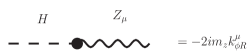
Figure 1: Feynman rule.

III The CPT-odd anomalous magnetic dipole moment

Having presented the structure of the Lagrangian of interest, we now turn to present the calculation of the vertex that involves the information on the $k_{\phi\,R}^{\mu}$ four vector. Let us consider the invariant amplitude

$$-i{\cal M}=\bar{u}(p_{2})\left(-i\Gamma_{\mu}\right)u(p_{1})\epsilon^{\mu*}(q),$$ (6)

where the vertex $\Gamma_{\mu}=\Gamma_{\mu}^{(a)}+\Gamma_{\mu}^{(b)}$ receives contributions at the one loop level from diagrams in Fig. 2 (a) and (b). For the $\Gamma_{\mu}^{(a)}$ contribution, we have

$$-i\Gamma_{\mu}^{(a)}=i\frac{eg^{2}m_{Z}^{2}}{\cos^{2}\theta_{W}}\int\frac{d^{4}k}{(2\pi)^{4}}\frac{T_{\mu}}{\left[k^{2}-m^{2}_{H}\right]\left[k^{2}-m^{2}_{Z}\right]^{2}\left[\left(k+p_{1}\right)^{2}-m^{2}_{l}\right]\left[\left(k+p_{2}\right)^{2}-m^{2}_{l}\right]},$$ (7)

with

$$T_{\mu} = (k_{\phi R})_{\lambda}(k_{\phi R})_{\beta}\left(g^{\alpha\beta}-\frac{k^{\alpha}k^{\beta}}{m_{Z}^{2}}\right)\left(g^{\beta\lambda}-\frac{k^{\beta}k^{\lambda}}{m_{Z}^{2}}\right)\bigg{[}\gamma_{\beta}\left(g_{V}^{f}-g_{A}^{f}\gamma^{5}\right)$$

$$\times(\hbox{\large$/$}\kern-5.76042pt\hbox{$k$}+\hbox{\large$/$}\kern-5.51563pt\hbox{$p$}_{2}+m_{l})\gamma_{\mu}(\hbox{\large$/$}\kern-5.76042pt\hbox{$k$}+\hbox{\large$/$}\kern-5.51563pt\hbox{$p$}_{1}+m_{l})\gamma_{\alpha}\left(g_{V}^{f}-g_{A}^{f}\gamma^{5}\right)\bigg{]}.$$ (8)

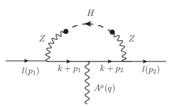
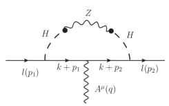
Figure 2: Feynman diagrams contributing to the $\bar{l}l\gamma$ vertex.

The contribution resulting from diagram in Fig. 2 (b) is quite suppressed due to the coupling $H\bar{l}l$ which is $\frac{igm_{l}}{2m_{W}}$, hence the corresponding amplitude is suppressed by a factor $\left(\frac{m_{l}}{m_{W}}\right)^{2}$ and, consequently, we can neglect it.

In order to carry out the calculations of the invariant amplitude ${\cal M}$ in Eq. (6) and the vertex function, $\Gamma^{\mu}$, we use the tensor decomposition of FeynCalc feyncalc to express the form factors in Eq. (1) in terms of Passarino-Veltman (PV) scalar functions. The result is quite lengthy and it depends on $A_{0}$, $B_{0}$, $C_{0}$ and $D_{0}$ PV scalar functions, in general with different arguments. Let us comment that at some stage of calculation, we used different identities of PV scalar functions such as $A_{0}(m^{2})=m^{2}[1+B_{0}(0,m^{2},m^{2})]$ in order to eliminate the $A_{0}$, $C_{0}$ and $D_{0}$ functions with proper arguments in favor of the $B_{0}$’s functions. Finally, the contribution due to CPT-odd coefficients to the AMDM, $a_{l}^{\mathrm{CPT-odd}}$ for a lepton $l$, can be cast as:

$$a_{l}^{\mathrm{CPT-odd}}=\frac{\alpha}{\pi\sin 2\theta_{W}}\left(\frac{m_{Z}^{2}}{m_{H}^{2}-m_{Z}^{2}}\right)\left(\frac{k_{\phi_{R}}^{2}}{m_{l}^{2}}\right)\left[(g_{V}^{l})^{2}f_{V}(0)+(g_{A}^{l})^{2}f_{A}(0)\right],$$ (9)

where, as usual, $\alpha=e^{2}/4\pi$ is the fine structure constant. We recall that $k_{\phi_{R}}^{2}=k_{\phi_{R}}^{\mu}k_{{\phi_{R}}\,\mu}$ and it can be positive, negative or zero. In the last case, nothing to do. Thus, we tacitly assume that $k_{\phi_{R}}^{\mu}$ can be either space-like or time-like four-vector. The vector $f_{V}(0)=f_{V}(q^{2}=0)$ and the axial $f_{A}(0)=f_{A}(q^{2}=0)$ form factors are given respectively by

$$f_{V,A}(0)=f_{0}^{V,A}+\sum_{i=1}^{5}f_{i}^{V,A}B_{0}(i)+f_{6}^{V,A}m_{Z}^{2}C_{0}.$$ (10)

Here, the various $B_{0}(i)$ functions stand for PV’s with different argument. The explicit expressions for the functions involved in this equation are displayed in the appendix. Although the dipole magnetic moment in Eq. (9) is expressed in a linear form, as a function of different $B_{0}$’s, each containing an UV divergence, its is easy to see that the final result is UV free, as it must be.

An analysis of the different functions in Eq. (10), indicates that the $a_{l}^{\mathrm{CPT-odd}}$ is very sensitive to the mass $m_{l}$ of the charged lepton. This implies that the main result emerges from the AMDM of the electron. The most important contributions to the vector and axial parts come from the terms $f_{1}^{V,A}B_{0}(1)$, $f_{2}^{V,A}B_{0}(2)$ and $f_{6}^{V,A}m_{Z}^{2}C_{0}$, respectively. Moreover a Taylor expansion around $m_{l}=0$ shows that the dominant contribution to $f_{V}(0)$ part is

$$f_{V}(0)=\frac{3}{8}\left(\frac{m_{Z}^{2}}{m_{e}^{2}}\right)\log\left(\frac{m_{Z}^{2}}{m_{e}^{2}}\right)+\cdots,$$ (11)

where the ellipsis stand for contributions ${\cal O}(m_{e}^{2}/m_{Z}^{2})$ which can be dropped. Analogously, the dominant contribution to the axial form factor comes from the electron:

$$f_{A}(0)=\frac{9}{32}\left(\frac{m_{Z}^{2}}{m_{e}^{2}}\right)\log\left(\frac{m_{Z}^{2}}{m_{e}^{2}}\right)+\cdots.$$ (12)

Hence, the main contribution to the electron AMDM arising from CPT-odd Higgs sector of the mSME can be written as

$$a_{e}^{\mathrm{CTP-odd}}=\frac{\alpha}{\pi\sin^{2}2\theta_{W}}\left(\frac{m_{Z}^{2}}{m_{H}^{2}-m_{Z}^{2}}\right)\left(\frac{|k_{\phi_{R}}^{2}|}{m_{e}^{2}}\right)\left[\frac{3}{8}\left(g_{V}^{e}\right)^{2}+\frac{9}{32}\left(g_{A}^{e}\right)^{2}\right]\left(\frac{m_{Z}^{2}}{m_{e}^{2}}\right)\log\left(\frac{m_{Z}^{2}}{m_{e}^{2}}\right),$$ (13)

where, for convenience and to compare with the experimental value of the AMDM of the electron, we have taken the absolute value of $k_{\phi,R}^{2}$. By demanding that $a_{e}^{\mathrm{CTP-odd}}$ be less than the experimental uncertainty: $a_{e}^{\mathrm{CTP-odd}}<\Delta a_{e}^{\mathrm{Exp}}$, we can establish a bound for the CPT-odd coefficient:

$$|k_{\phi_{R}}^{2}|<\left\{\frac{\alpha}{\pi\sin^{2}2\theta_{W}}\left(\frac{m_{Z}^{4}}{m_{H}^{2}-m_{Z}^{2}}\right)\left[\frac{3}{8}\left(g_{V}^{e}\right)^{2}+\frac{9}{32}\left(g_{A}^{e}\right)^{2}\right]\log\left(\frac{m_{Z}^{2}}{m_{e}^{2}}\right)\right\}^{-1}m_{e}^{4}\,\,\Delta a_{e}^{\mathrm{Exp}}.$$ (14)

In order to determine the numerical bound, we use the values reported in the Particle Data Group pdg for different parameter in the expression, finding that $|k_{\phi_{R}}^{2}|<3.29\times 10^{-29}$ GeV².

IV Conclusions and final considerations

The mSME is a minimal extension to the standard model that accounts for the violations of the Lorentz and CTP symmetries that could occur in nature. The corresponding Lagrangian contains terms composed by CPT-even and CPT-odd coefficients that couple to matter and gauge fields. The knowledge of these coefficients could be helpful to find out in a more exhaustive way the possible violations of the mentioned symmetries. In this paper we have presented a calculation on the contributions arising from the CPT-odd Higgs sector of the mSME to the AMDM of charged leptons. We found that, in the limit $m_{l}\ll m_{H},m_{Z}$, the dominant contribution is due to the lighter lepton. For the case of an electron, we obtained an analytical expression for the AMDM that takes into account the effects of the CPT-odd background resulting from the sector under consideration. This allowed us to establish the bound on the CPT-odd coefficient: $|\,k^{2}_{\phi\,R}|<3.29\times 10^{-29}$ GeV².

Appendix A

Useful relation between Passarino-Veltman scalar functions.

$$B_{0}(1)= B_{0}(m_{l}^{2},m_{l}^{2},m_{Z}^{2})$$

$$B_{0}(2)= B_{0}(m_{l}^{2},m_{l}^{2},m_{H}^{2})$$

$$B_{0}(3)= B_{0}(0,m_{Z}^{2},m_{Z}^{2})$$

$$B_{0}(4)= B_{0}(0,m_{H}^{2},m_{H}^{2})$$

$$B_{0}(5)= B_{0}(0,m_{H}^{2},m_{H}^{2})$$

$$C_{0}\equiv C_{0}(m_{l}^{2},0,0,m_{Z}^{2},m_{l}^{2},m_{Z}^{2})$$

$$= \frac{\partial}{\partial m_{Z}^{2}}\frac{1}{i\pi^{2}}\int d^{4}k\frac{1}{(k^{2}-m_{Z}^{2})[(k+p_{1})^{2}-m_{l}^{2}]}$$

$$= \frac{1}{m_{l}^{2}\sqrt{1-\frac{4m_{l}^{2}}{m_{Z}^{2}}}}\left[-\frac{1}{2}\sqrt{1-\frac{4m_{l}^{2}}{m_{Z}^{2}}}\log\left(\frac{m_{Z}^{2}}{m_{l}^{2}}\right)+\left(1-\frac{2m_{l}^{2}}{m_{Z}^{2}}\right)\log\left(\frac{1-\sqrt{1+\frac{4m_{l}^{2}}{m_{Z}^{2}}}}{1-\sqrt{1-\frac{4m_{l}^{2}}{m_{Z}^{2}}}}\right)\right]$$

Vector form factors:

$$f_{0}^{V}= \frac{1}{(m_{H}^{2}-4m_{l}^{2})(m_{Z}^{2}-4m_{l}^{2})^{2}(m_{H}^{2}-m_{Z}^{2})}\bigg{\{}-\frac{7}{4}m_{H}^{2}m_{Z}^{4}(m_{H}^{2}-m_{Z}^{2})$$

$$+m_{l}^{2}\left[4m_{l}^{2}(m_{H}^{2}-m_{Z}^{2})(16m_{l}^{2}-15m_{Z}^{2})+m_{Z}^{2}(11m_{H}^{4}-4m_{Z}^{2}m_{H}^{2}-7m_{Z}^{4})\right]\bigg{\}}$$

$$f_{1}^{V}= \frac{1}{4(m_{Z}^{2}-4m_{l}^{2})^{2}(m_{H}^{2}-m_{Z}^{2})}\bigg{\{}m_{Z}^{4}(13m_{H}^{2}-5m_{Z}^{2})$$

$$+2m_{l}^{2}\left[4m_{l}^{2}(17m_{H}^{2}-5m_{Z}^{2})-m_{Z}^{2}(47m_{H}^{2}-19m_{Z}^{2})\right]\bigg{\}}$$

$$f_{2}^{V}= -\frac{2m_{H}^{2}(m_{H}^{2}-3m_{l}^{2})}{(m_{H}^{2}-m_{l}^{2})(m_{H}^{2}-m_{Z}^{2})}$$

$$f_{3}^{V}= -\frac{1}{4(m_{Z}^{2}-4m_{l}^{2})^{2}(m_{H}^{2}-m_{Z}^{2})}\bigg{\{}m_{Z}^{4}(13m_{H}^{2}-5m_{Z}^{2})$$

$$+2m_{l}^{2}\left[m_{l}^{2}m_{H}^{2}+12m_{Z}^{2}(3m_{Z}^{2}-7m_{H}^{2})\right]\bigg{\}}$$

$$f_{4}^{V}= \frac{m_{l}^{2}}{2(m_{H}^{2}-4m_{l}^{2})(m_{Z}^{2}-4m_{l}^{2})^{2}}\bigg{\{}4m_{l}^{2}(20m_{l}^{2}-9m_{H}^{2}-m_{Z}^{2})+5m_{H}^{2}m_{Z}^{2}\bigg{\}}$$

$$f_{5}^{V}= \frac{2m_{H}^{2}(m_{H}^{2}-2m_{l}^{2})}{(m_{H}^{2}-4m_{l}^{2})(m_{H}^{2}-m_{Z}^{2})}$$

$$f_{6}^{V}= \frac{3m_{Z}^{2}-4m_{l}^{2}}{4(m_{Z}^{2}-4m_{l}^{2})}$$

Axial form factors:

$$f_{0}^{A}= \frac{1}{48m_{Z}^{4}(m_{Z}^{2}-4m_{l}^{2})}\bigg{\{}m_{Z}^{2}\left[16m_{H}^{2}(3m_{H}^{2}-m_{Z}^{2})-85m_{Z}^{4}\right]$$

$$+2m_{l}^{2}\left[4m_{l}^{2}(33m_{H}^{2}-73m_{Z}^{2})-m_{H}^{2}(96m_{H}^{2}+m_{Z}^{2})+195m_{Z}^{4}\right]\bigg{\}}$$

$$f_{1}^{A}= \frac{1}{48m_{Z}^{2}(m_{Z}^{2}-4m_{l}^{2})^{2}(m_{H}^{2}-m_{Z}^{2})}\bigg{\{}5m_{Z}^{4}(33m_{H}^{2}-17m_{Z}^{2})$$

$$+2m_{l}^{2}\left[4m_{l}^{2}(93m_{H}^{2}-29m_{Z}^{2})-m_{Z}^{2}(399m_{H}^{2}-175m_{Z}^{2})\right]\bigg{\}}$$

$$f_{2}^{A}= \frac{1}{48m_{Z}^{4}(m_{H}^{2}-m_{Z}^{2})}\bigg{\{}-16m_{H}^{2}(3m_{H}^{4}-4m_{H}^{2}m_{Z}^{2}+6m_{Z}^{4})$$

$$+32m_{l}^{2}(3m_{H}^{4}-2m_{H}^{2}m_{Z}^{2}+3m_{Z}^{4})\bigg{\}}$$

$$f_{3}^{A}= \frac{1}{48m_{Z}^{2}(m_{Z}^{2}-4m_{l}^{2})(m_{H}^{2}-m_{Z}^{2})}\bigg{\{}-5m_{Z}^{4}(33m_{H}^{2}-17m_{Z}^{2})$$

$$-4m_{l}^{2}\left[48m_{l}^{2}(2m_{H}^{2}-m_{Z}^{2})+m_{Z}^{2}(73m_{Z}^{2}+165m_{H}^{2})\right]\bigg{\}}$$

$$f_{4}^{A}= \frac{m_{l}^{2}}{48m_{Z}^{4}(m_{H}^{2}-m_{Z}^{2})}\bigg{\{}8m_{l}^{2}(24m_{H}^{2}-53m_{Z}^{2})-2m_{Z}^{2}(24m_{H}^{2}-77m_{Z}^{2})\bigg{\}}$$

$$f_{5}^{A}= \frac{1}{48m_{Z}^{4}(m_{H}^{2}-m_{Z}^{2})}\bigg{\{}16m_{H}^{2}(3m_{H}^{4}-4m_{H}^{2}m_{Z}^{2}+6m_{Z}^{4})-48m_{l}^{2}m_{Z}^{4}\bigg{\}}$$

$$f_{6}^{A}= \frac{9}{16}-\frac{m_{l}^{2}}{4m_{Z}^{2}}$$

References

- (1) D. Colladay and V. A. Kostelecký, Phys. Rev. D55, 6760 (1997).
- (2) V. A. Kostelecký, Phys. Rev. D69, 105009 (2004).
- (3) D. Colladay and V. A. Kostelecký, Phys. Rev. D58, 116002 (1998).
- (4) D. Colladay, P. McDonald, J. P. Noordmans, and R. Potting, Phys. Rev. D 95, 025025 (2017).
- (5) V. Alan Kostelecký and Matthew Mewes, Astrophys. J. 611, L1 (2008).
- (6) V. A. Kostelecký and M. Mewes, Phys. Rev. D70, 031902(R) (2004).
- (7) M. C. D. Torri, Universe 6, 37 (2020).
- (8) DUNE Collaboration, B. Abi et al., Eur.Phys. J. C 81, 322 (2021).
- (9) S. Sahoo, A. Kumara, and S. K. Agarwalla, JHEP 03, 050 (2022).
- (10) H-X. Lin, J. Tang, S. Vihonen, and P. Pasquini, Phys. Rev. D 105, 096029 (2022).
- (11) V. A. Kostelecký and N. Russell, Rev. Mod. Phys. 83, 11 (2011); arXiv:0801.0287V15.
- (12) J. I. Aranda, F. Ramírez-Zavaleta, D. A. Rosete, F. J. Tlachino, J. J. Toscano and E. S. Tututi, J. Phys. G: Nucl. Part. Phys. 41 055003 (2014).
- (13) J. I. Aranda, F. Ramírez-Zavaleta, F. J. Tlachino, J. J. Toscano and E. S. Tututi, Int. J. Mod. Phys. A 29, 1450180 (2014).
- (14) D. L. Anderson, M. Sher, and I. Turan, Phys. Rev. D70, 016001 (2004).
- (15) A. I. Hernández-Juárez, J. Montaño, H. Novales-Sánchez, M. Salinas, J. J. Toscano and O. Vázquez-Hernández, Phys. Rev. D99, 013002 (2019).
- (16) J. A. Ahuatzi-Avendaño, J. Montaño, H. Novales-Sánchez, M. Salinas and J. J. Toscano, Phys. Rev. D103, 055003 (2021).
- (17) J. Montaño-Domínguez, H. Novales-Sánchez, M. Salinas and J. J. Toscano, Phys. Rev. D105, 075018 (2022).
- (18) D. Bear, R. E. Stoner, R. L. Walsworth, V. A. Kostelecký, and Charles D. Lane, Phys. Rev. Lett. 85, 5038 (2000); ibid Phys. Rev. Lett. 89, 909902(E) (2002).
- (19) M. Nowakowski, E. A. Paschos, and J. M. Rodríguez,Eur. J. Phys. 26, 545 (2005).
- (20) R. Mertig, M. Böhm, and A. Denner, Comput. Phys. Commun. 64, 345 (1991).
- (21) P. A. Zyla et. al., [Particle Data Group],Prog. Theor. Exp. Phys. 2020, 083C01 (2020).