Can Carbon Fractionation Provide Evidence for Aerial Biospheres in the Atmospheres of Temperate Sub-Neptunes?

Abstract

The search for signs of life on other worlds has largely focused on terrestrial planets. Recent work, however, argues that life could exist in the atmospheres of temperate sub-Neptunes. Here, we evaluate the usefulness of carbon dioxide isotopologues as evidence of aerial life. Carbon isotopes are of particular interest as metabolic processes preferentially use the lighter ¹²C over ¹³C. In principle, the upcoming James Webb Space Telescope (JWST) will be able to spectrally resolve the ¹²C and ¹³C isotopologues of CO₂, but not CO and CH₄. We simulated observations of CO₂ isotopologues in the H₂-dominated atmospheres of our nearest ($<40$ pc), temperate (equilibrium temperature of 250-350 K) sub-Neptunes with M dwarf host stars. We find ¹³CO₂ and ¹²CO₂ distinguishable if the atmosphere is H₂-dominated with a few percentage points of CO₂ for the most idealized target with an Earth-like composition of the two most abundant isotopologues, ¹²CO₂ and ¹³CO₂. With a Neptune-like metallicity of 100$\times$ solar and a C/O of 0.55, we are unable to distinguish between ¹³CO₂ and ¹²CO₂ in the atmospheres of temperate sub-Neptunes. If atmospheric composition largely follows metallicity scaling, the concentration of CO₂ in a H₂-dominated atmosphere will be too low to distinguish CO₂ isotopologues with JWST. In contrast, at higher metallicities, there will be more CO₂, but the smaller atmospheric scale height makes the measurement impossible. Carbon dioxide isotopologues are unlikely to be useful biosignature gases for the JWST era. Instead, isotopologue measurements should be used to evaluate formation mechanisms of planets and exoplanetary systems.

1 Introduction

So far the search for signs of life on other worlds has focused on terrestrial planets, but recent work has explored whether life could originate and survive in the liquid water clouds of temperate sub-Neptune-sized planets (Seager et al., 2021). Sub-Neptunes are more readily observable than terrestrial planets due to their larger size and low mean molecular weight (MMW), H₂-dominated atmospheres (e.g., Bean et al., 2021). Passive microbial-like particles could persist aloft in regions with liquid water clouds for long enough to metabolize, reproduce, and spread before sinking to altitudes that may be too hot for life of any kind to survive (Seager et al., 2021). Isotope fractionation is thought to be among the strongest signs of life that theoretically can be remotely detected in a planet’s atmosphere (Neveu et al., 2018). On Earth, carbon isotope fractionation has been used as evidence of early life as biotic deposits of carbon have a higher ratio of ¹²C/¹³C than abiotic deposits (e.g., Rothschild & Desmarais, 1989). The key metabolic processes that fractionate carbon are photosynthesis, chemosynthesis, respiration, and decomposition of organic matter (e.g., Mackenzie & Lerman, 2006). Isotopic compositions, however, can also be changed by geophysical or chemical processes (e.g., degassing of basaltic magma (Mattey, 1991) and chemical exchange in the protoplanetary disk (Woods & Willacy, 2009)).

The upcoming James Webb Space Telescope (JWST) (Gardner et al., 2006), launched on December 25, 2021, provides an opportunity to characterize exoplanets using isotopologues. JWST is predicted to be able to make measurements of the protosolar D/H ratio ($2\times 10^{-5}$) using the methane isotopologue, CH₃D, for nearby, cool brown dwarfs in just 2.5 hr of JWST observing time (Morley et al., 2019). In addition, oxygen isotopes could be used to look for evidence of ocean loss. Simulated observations suggest that JWST could observe oxygen isotopologues in water and carbon dioxide molecules in the atmospheres of terrestrial planets around the M dwarf star TRAPPIST-1. The oxygen isotopic ratio, ¹⁸O/¹⁶O, can be used as a marker of ocean loss and atmospheric escape as the lighter ¹⁶O is preferentially removed from photodissociated water vapor. Simulated JWST observations show that we may be able to distinguish Venus-like fractionation ($\delta^{18}$O 100) potentially caused by massive ocean loss from Earth-like fractionation in as little as 4 transits for TRAPPIST-1b and 5 transits for TRAPPIST-1d (Lincowski et al., 2019).

From the ground, high-resolution data can be used to detect isotopologues via direct imaging and spectroscopy. Recently, ¹³CO became the first carbon isotopologue to be measured in an exoplanet’s atmosphere (Zhang et al., 2021). Using the SINFONI instrument on the Very Large Telescope (VLT), Zhang et al. (2021) observed the atmosphere of super-Jupiter TYC 8998-760-1 b and found a ¹²CO/¹³CO ratio of $31^{+17}_{-10}$ (90% confidence) in contrast to our solar system average ratio of approximately 89 (Woods & Willacy, 2009) and local interstellar medium value of about 68 (Milam et al., 2005). Zhang et al. (2021) attribute the significant ¹³C enrichment to the formation location of the planet past the CO snowline where isotopic ion-exchange reactions and isotope-selective photodissociation can lead to an enhancement in ¹³C in CO ice compared to CO gas.

Additionally, simulations of high-resolution observations of ¹³C¹⁶O, HDO, and CH₃D have been created based on models of the CRyogenic InfraRed Echelle Spectrograph Upgrade (CRIRES+) instrument on the Very Large Telescope (VLT) and the Mid-infrared ELT Imager and Spectrograph (METIS) instrument on the upcoming Extremely Large Telescope (ELT) (Molliere & Snellen, 2019). ¹³C¹⁶O was detectable in the dayside emission of hot Jupiters using the simulated VLT observation (Molliere & Snellen, 2019). 40 m-class telescopes, like the ELT, might make detection of CH₃D possible for cool planets (Molliere & Snellen, 2019). CH₃D might also be detectable in nearby super-Earths if they are irradiated or transiting (Molliere & Snellen, 2019). However, HDO observations may be hampered by methane absorption, which occurs at similar wavelengths. The ELT will likely be necessary for observations of HDO unless the methane is quenched (Molliere & Snellen, 2019).

We extend past work to focus on assessing the usefulness of isotopologues as biosignature gases. Here, we quantify the detectability of ¹²C/¹³C via CO₂ in the atmospheres of nearby sub-Neptunes. We choose sub-Neptunes as they are more readily observable than super-Earths due to their larger size and low MMW, H₂-dominated atmospheres. We choose carbon dioxide isotopologues as carbon is fractionated by life, and the spectral separation of ¹²CO₂ from ¹³CO₂ is theoretically large enough to be resolved with JWST. In Section 2, we explain how we modeled the detection of isotopologues using spectra generated with petitRADTRANS (Mollière et al., 2019) and a simulated JWST noise model using PandExo (Batalha et al., 2017). In Section 3, we show our results and explain how we assessed detectability. In Section 4, we expound on the significance of our findings and evaluate the usefulness of isotopologues as biosignature gases in exoplanetary atmospheres. Our framework is designed to assess if carbon fractionation is a detectable biosignature gas or if the technology needed will be out of reach for decades to come. Knowing what kinds of measurements we can and cannot make will help guide future mission development.

2 Methods

We used petitRADTRANS to generate simulated spectra. petitRADTRANS (Mollière et al., 2019) is a well validated Python package to generate transmission spectra that has been broadly accepted by the community. As input to petitRADTRANS, we calculated ¹³CO₂ isotopologues cross sections using ExoCross (Yurchenko et al., 2018) from input line list that are available publicly on the High-Resolution Transmission Molecular Absorption (HITRAN) database (Gordon et al., 2017). We use the temperature-pressure profile of temperate sub-Neptune K2-18b by Blain et al. (2021). We calculate chemical abundances using the chemical equilibrium implementation from petitRADTRANS. The chemical abundances of the dominant volatiles at 1 bar are used as input boundary conditions to our photochemical model of the atmosphere.

Our photochemistry model (Hu et al., 2012) is a simplified one-dimensional chemical transport model. By calculating the atmosphere’s steady-state chemical compositions, our model can simulate a variety of atmospheres, such as H₂-dominated reducing atmospheres and CO₂-dominated highly oxidizing atmospheres. The photochemistry model has been validated by simulating modern Earth’s and Mars’ atmospheres (Hu et al., 2012). For more detailed information and applications of our model see Hu et al. (2012, 2013); Seager et al. (2013); Sousa-Silva et al. (2020); Zhan et al. (2021); Huang et al. (2022).

Our fiducial sub-Neptune atmosphere for the photochemical model is an H₂-dominated, Neptune-like atmosphere ([M/H]=100, C/O=0.55) orbiting an M dwarf star. We adopt the mass and radius of K2-18 b to describe the planet and the M dwarf stellar radiation model of GJ 876 (France et al., 2016; Loyd et al., 2016). Our simulated atmosphere consists of two segments: a lower convective layer ($10^{5}$ Pa to $10^{-1}$ Pa) and an upper radiative layer ($<10^{-1}$ Pa). (The two segments are unrelated to our 100-layer atmosphere model used to simulate the transmission spectrum.) The temperature-pressure profile of the convective layer comes from Figure 4 of Blain et al. (2021). Since we do not consider heating in the upper atmosphere, we assume the temperature to be constant (isothermal) in the upper radiative layer. In our photochemistry model, the vertical mixing processes are parameterized by the atmosphere’s eddy diffusion coefficient ($K_{zz}$). We use the free-convection and mixing-length theories (Stone, 1976; Flasar & Gierasch, 1977; Gierasch & Conrath, 1985; Visscher & Moses, 2011) to help us constrain the value of $K_{zz}$. However, the constraints are loose, and hence we tested the impact of using a range of values of K_zz, $1\times 10^{8}$ to $1\times 10^{10}$ (Gierasch & Conrath, 1985; Visscher & Moses, 2011; Hu & Seager, 2014). We found that the K_zz did not change our column averaged mixing ratios. In our fiducial simulation run, we adopt a uniform K_zz of $1\times 10^{9}$ cm²s^-1, a value also adopted by Moses et al. (2013); Miguel & Kaltenegger (2013), and Hu & Seager (2014). In our simulation, we include all the reactions mentioned in Hu et al. (2012), except for HSO₂ thermal decay, high-temperature reactions, and reactions that involve more than two carbon atoms (Hu et al., 2012). Given our choice of the temperature-pressure profile, we omit NH₄SH and NH₃ aerosols since the atmosphere is too hot for them to condense (Hu, 2021). Furthermore, we do not consider rainout in our simulation as there is no ocean and the temperature at the bottom of our simulated atmosphere is such that any rain will inevitably evaporate.

Using the results of our photochemistry model, we simulate observations of the Near Infrared Spectrograph (NIRSpec) Instrument on JWST. NIRSpec covers 0.6 to 5.3 $\mu$m (STScI, 2020). Using the PRISM disperser, the entire bandpass can be measured at a resolution of R$\approx$100. For high-resolution observations at an R$\approx$2700, we simulate the G395H disperser over the range of 2.87 $\mu$m to 5.27 $\mu$m (STScI, 2020).

We calculate the anticipated on-orbit noise for JWST using the Space Telescope Science Institute Exposure Time Calculator for Exoplanets, PandExo (Batalha & Line, 2017). PandExo performs throughput calculations using the Space Telescope Science Institute’s (STScI) Pandeia. Schlawin et al. (2021) estimated the magnitude of the noise for NIRCam, which has similar systematic error to NIRSpec. They found that the pointing uncertainty and jitter will be less than 6 ppm; thermal instabilities in the optics will be less than 2 ppm; persistence will be less than 3 ppm; and detector temperature fluctuations will be about 3 ppm. Given the sources of uncertainties, we adopt a noise floor of 10 ppm for our model. To further configure our noise model, we set an 80% saturation level for each pixel. We also set the in-transit time equal to the out-of-transit time. We use input stellar spectrum from PHOENIX (Husser et al., 2013) based on the magnitude, temperature, metallicity, and surface gravity of the host star. In addition, we define the properties of the planet and host star.

3 Results

We present exoplanet transmission spectra with and without ¹³CO₂ in order to quantify the detectability of carbon isotopic composition in the atmosphere of a sub-Neptune-sized exoplanet with JWST. When ¹³C is included, we assume Earth-like fractionation.

3.1 Detection of Carbon Isotopes in an Ideal Target

We find ¹³CO₂ to be detectable with JWST for the most idealized, simulated target. To best distinguish ¹³CO₂ from ¹²CO₂ the atmospheric composition needs to be predominately hydrogen gas with trace amounts of carbon dioxide. Benneke et al. (2019) found that K2-18 b has a H₂-dominated, a low MMW (2.42) atmosphere that contains water. While Benneke et al. (2019) did not conclusively detect other gases, they were able to place upper limits on CO, CO₂, NH₃, and CH₄ gas. We simulated an observation using a similar atmospheric composition based on the low MMW and upper limits. We found ¹³CO₂ was distinguishable from ¹²CO₂ at an SNR of 9.1 after a 10 transit observation as seen in Figure 1. However, this result holds only for the most ideal artificial target of the sub-Neptune TOI-1231 b placed around our nearest M dwarf host star, LTT 1445 A. We are unable to distinguish ¹³CO₂ from ¹²CO₂ for any of the real temperate sub-Neptune targets.

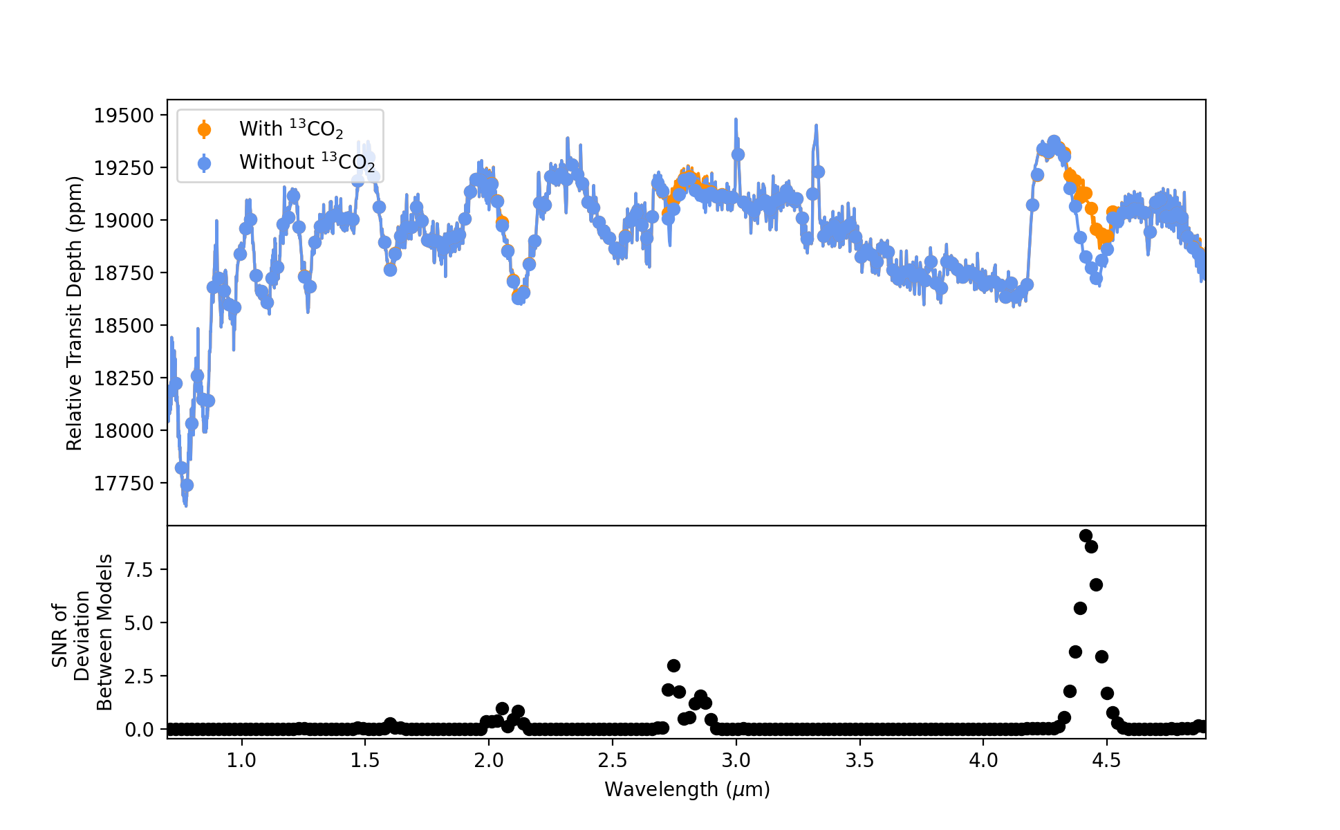
Figure 1: Simulated observation of the sub-Neptune TOI-1231 b artificially placed around our nearest M dwarf host star, LTT 1445 A, observed in the PRISM mode for 10 transits. The simulated atmosphere has an MMW of 2.42 and contains similar molecular abundances to those found in K2-18 b (Benneke et al., 2019). The upper panel shows the relative transit depth in parts per million (ppm) for the wavelengths associated with JWST’s PRISM mode. The blue spectrum does not include ¹³CO₂ while the orange one does. The lower panel shows the signal to noise ratio (SNR) of the deviation between the models with and without ¹³CO₂. As seen in lower panel, for a 10 transit observation, the SNR value is 9.1.

3.2 Non-Detection of Carbon Isotopes in Simulated Sub-Neptune Atmospheres

Our results show that we we will not be able to distinguish between carbon dioxide isotopologues for known temperate sub-Neptunes regardless of the atmospheric composition. We construct an atmosphere with a Neptune-like metallicity of 100x solar and a C/O ratio of 0.55 using our photochemistry model. We simulate a 10 transit observation for our most readily observable, temperate sub-Neptune, TOI-1231 b, with JWST’s PRISM mode as shown in Figure 2. The upper panel shows the relative transit depth in parts per million (ppm) over the wavelength coverage of the PRISM mode (R $\sim$ 100). The blue spectrum includes only CO₂ with ¹²C while the orange spectrum also includes ¹³CO₂. The lower panel shows the signal-to-noise ratio of the deviation between the models or how well we would be able to distinguish observing CO₂ with and without ¹³C. The SNR for a 10 transit observation is very low at 0.2.

We also simulated observations of LHS 1440 b, K2-18 b, and an artificial sub-Neptune around our closest M dwarf host star, LTT 1445 A. In all cases, we found we were unable to distinguish between our models with and without ¹³CO₂. The SNR of the deviation between the model with and without ¹³CO₂ for the four different planets is shown in Figure 3. The planets are listed in the rows, and the number of transits observed changes with the columns. The first planet listed is an artificial planet, a sub-Neptune around the closest known M dwarf host star LTT 1445 A. (In reality, LTT 1445 A b is a 1.38 R_Earth super-Earth, not a sub-Neptune.)

We also tested the impact of varying the metallicity of the atmosphere and found that there is no “sweet spot” between a low MMW atmosphere and a CO₂ abundance that allowed for a positive detection of ¹³CO₂ if the atmosphere followed metallicity scaling. The range of possible sub-Neptune atmospheric compositions remains largely unknown (Bean et al., 2021, and references therein). The compositions are believed to be H₂ dominated, though the metallicity range remains uncertain. While a lower metallicity atmosphere has a larger scale height, making it more readily observable, it comes at the cost of decreased CO₂ gas. A more metal-rich atmosphere would increase the amount of CO₂, but would also increase the MMW of the atmosphere, thus shrinking the scale height of the atmosphere and making it harder to detect overall, mostly due to large amounts of the heavy molecules, water and methane. Fortunately, CO₂ has a relatively large cross section, making it detectable at relatively low concentrations. In addition, carbon fractionation between the most abundant isotopologue and second must abundant isotopologue is relatively large at Earth-like fractionation. The carbon isotopologues of CO₂ are well separated compared with those of methane and carbon monoxide, allowing them to be potentially distinguishable even at low (R$\sim 100$) spectral resolution such as with JWST.

Currently, there are only four known nearby, temperate sub-Neptunes. LHS 1140 b is the closest at 12.47 $\pm$ 0.42 pc, but it is small for a sub-Neptune, right at the accepted cutoff between super-Earth and sub-Neptune at 1.727 $\pm$ 0.032 R_E (Dittmann et al., 2017; Ment et al., 2019). It has an estimated equilibrium temperature of 235.0 $\pm$ 5 K (Ment et al., 2019). TOI-270 d is the next closest at 22.453 $\pm$ 0.021 pc and it has an estimated equilibrium temperature of 340 $\pm$ 14 K (Günther et al., 2019). Farther away, TOI-1231 b is located at 27.4932 $\pm$ 0.0123 pc and has an equilibrium temperature of 330.0 $\pm$ 3.8 K (Burt et al., 2021). Lastly, K2-18 bis located at 38.07 $\pm$ 0.08 pc and has an estimated equilibrium temperature of 284 $\pm$ 15 K (Sarkis et al., 2018).

As more TESS Targets of Interest (TOIs) become validated planets, it is likely that additional temperature sub-Neptunes around nearby, bright M dwarfs, emerge as better targets. However, additional temperate sub-Neptunes will not prove amenable to isotopologue detection with JWST if the atmospheres follow solar metallicity scaling.

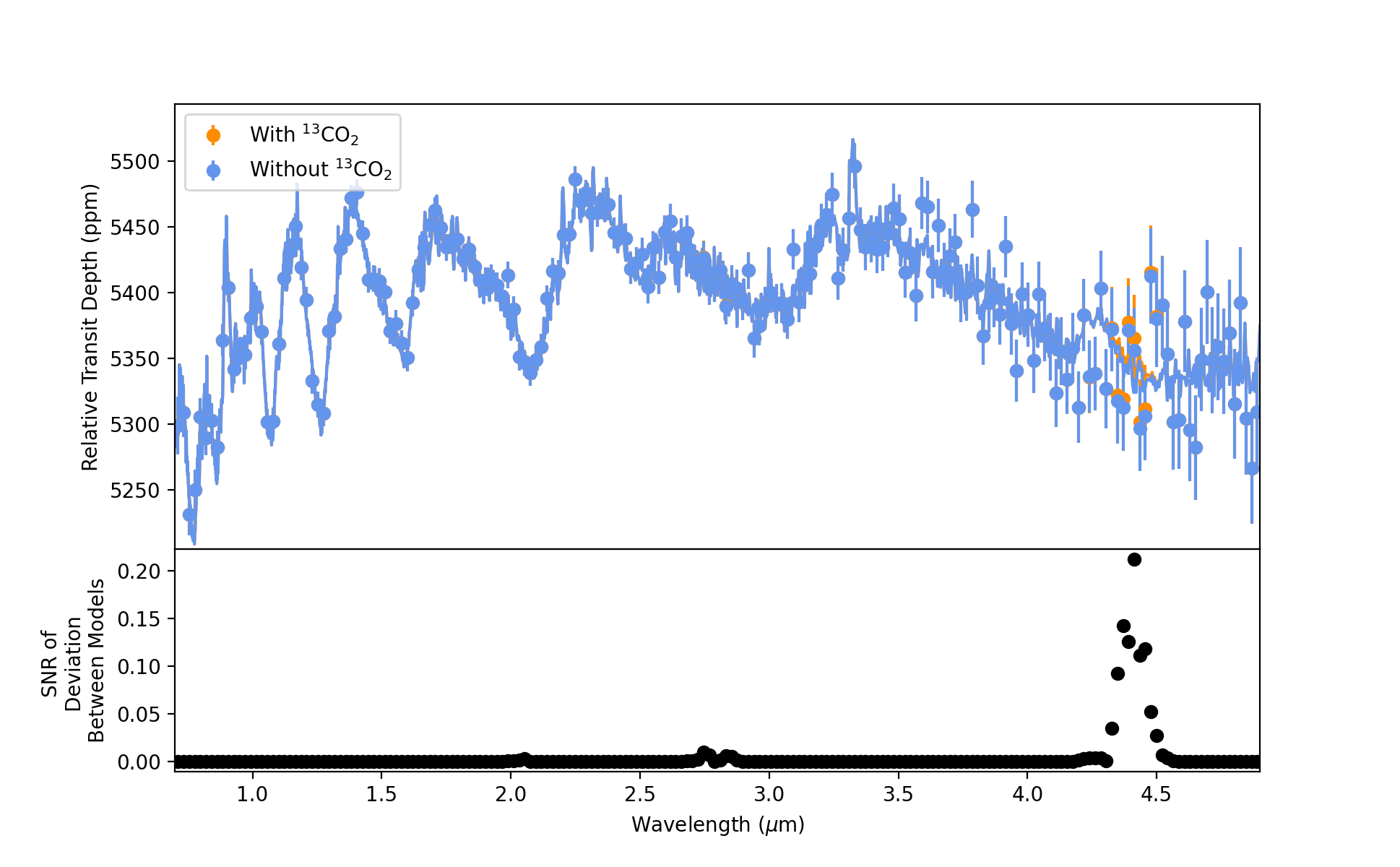
Figure 2: Simulated 10 transit, PRISM mode observation of TOI-1231 b with a Neptune-like metallicity of 100$\times$ solar and a C/O ratio of 0.55. The upper panel shows the relative transit depth in parts per million (ppm) for the wavelengths associated with JWST’s PRISM mode. The blue spectrum does not include ¹³CO₂ while the orange one does. The lower panel shows the signal to noise ratio (SNR) of the deviation between the models with and without ¹³CO₂. As seen in lower panel, for a 10 transit observation, the SNR value is low at 0.2.

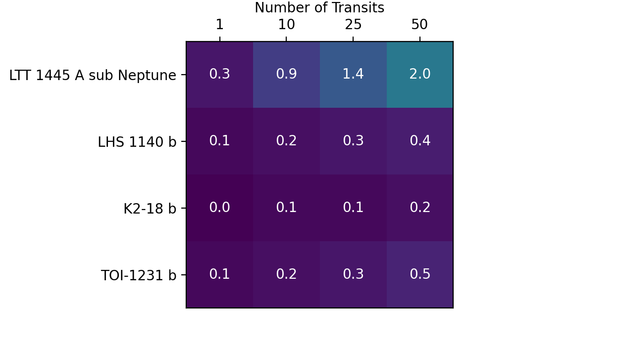
Figure 3: Summary plot of the SNR of the deviation between models that include ¹³C via CO₂ vs those that do not for an atmosphere with a Neptune-like metallicity of 100x solar and C/O of 0.55. The row labels show the names of the simulated target planets. The first planet is our artificial sub-Neptune (TOI-1231 b) around our closest known M dwarf host star LTT 1445 A, which in reality is host to a super-Earth, not a sub-Neptune. The column labels show the numbers of transits observed, from 1 to 50. A 10 transit observation is roughly the longest reasonable observation with JWST. The colors of the boxes correspond to the SNR value shown in each box where low values are cool colors with purple representing the lowest values. The SNR values range from 0.0 to 2.0, indicating that ¹³CO₂ is not detectable for a Neptune-like 100x solar metallicity atmosphere for even the most ideal, artificial sub-Neptune.

3.3 Non-Detectability at Higher Spectral Resolution

We also simulated observations using JWST’s high-resolution G395H disperser. The simulations revealed that our inability to distinguish ¹³CO₂ from ¹²CO₂ is not limited by the PRISM modes’ lower resolution, but by the number of photons received during the observation. In the high-resolution mode, the number of photons per bin decreased, leading to increased noise that obscured the spectral differences between ¹³CO₂ and ¹²CO₂.

3.4 Evaluation of Ground-based Observations

We also considered high-resolution ground-based observations of our targets. The velocity of our proposed targets is not a limiting issue. However, the cross-correlation technique will not be possible for temperate sub-Neptunes as the contrast between planet and star is too small for current giant telescopes. The SNR in the photon limited regime can be calculated as

$$\text{SNR}_{\text{planet}}=\frac{\text{S}_{\text{p}}}{\text{S}_{*}}\text{SNR}_{\text{star}}\sqrt{\text{N}_{\text{lines}}}$$

(Birkby, 2018). A coronagraph on a large ground-based telescope may allow for low-contrast observations in the future. Currently though, JWST is the best near-future instrument for measuring carbon dioxide isotopologues in the atmospheres of temperate planets.

4 Discussion

Even if someday we can detect carbon fractionation via ¹³CO₂, it will be nearly impossible to prove that it is caused by life and not by another process. Today, we do not even have a clear understanding of the composition of sub-Neptune atmospheres. Much of the early observations with JWST will simply focus on first assessing if small planets have atmospheres or not and then on measuring their atmospheric composition.

4.1 The Challenge of Disentangling Abiotic and Biotic Isotope Fractionation

A major complication of using isotopologues as biosignature gases is disentangling abiotic and biotic isotope fractionation. While isotope fractionation could be a strong indicator of life that is able to be detected remotely with the right instrument, we need to understand the context to rule out false positive detections (Neveu et al., 2018). The context includes both a habitability assessment of a planet and our understanding of abiotic fractionation processes. The magnitude of the fractionation alone will not be enough to unambiguously disentangle different biotic and abiotic fractionation processes.

On Earth, isotopic fractionation is measured by comparing the isotopic composition of a biotic carbon reservoir against an inorganic carbon reservoir. The composition of one isotope compared to another is not a biosignature on its own–it must be compared to a baseline inorganic value.

4.1.1 Abiotic Carbon Fractionation

Carbon fractionation occurs abiotically through processes such as chemical exchange reactions, photodissociation, gas release, and the kinetic isotope effect (Quay et al., 1991; Woods & Willacy, 2009). One known planetary process that fractionates carbon is volcanism (Mattey, 1991). The degassing of basaltic magma enriches the melt in ¹²CO₂, while enhancing the gas in ¹³CO₂ (Mattey, 1991). The magnitude of this effect is only $\sim 2$‰(Mattey, 1991). Our only example of a habitable planet (Earth) is subject to volcanic activity. Thus, carbon fractionation through magma outgassing will likely prove an important false positive that will need to be disentangled from biotic fractionation.

Another possible cause of fractionation could be differences in bulk isotopic composition between the remote exosystem and our own. If for instance, the solar system formed in an area near intermediate-mass AGB stars, it would be enriched in ¹³C (Kobayashi et al., 2011). Understanding the composition of the baseline abiotic carbon reservoir is the key to being able to interpret atmospheric measurements of ¹³CO₂.

4.1.2 Using Carbon Fractionation via Methane to Rule Out False Positives

Detection of carbon fractionation in an exoplanetary atmosphere can only be considered a sign of life if we have a full understanding of its context. While biologically mediated fractionation of carbon dioxide through photosynthesis is too subtle to be detectable, other carbon-bearing species like CH₄ or CO may prove more amenable for fractionation studies.

In contrast to our work assessing biologically fractionated carbon via CO₂, Molliere & Snellen (2019) suggested that metabolic carbon fractionation could be measured by comparing the composition of ¹³C vs ¹²C in CO₂ vs CH₄. Isotopic composition via CO₂ would serve as the baseline inorganic carbon reservoir while isotopic composition via CH₄ would be considered the organic carbon reservoir. Thus, an important application of our framework could be to assess the detectability of carbon fractionation via methane. However, as the spectral resolution required is too high for JWST and the contrast between host star and temperate planet is too low for ground-based high-resolution observations, the path forward to measure biologically driven isotope fractionation seems bleak.

4.2 Metabolic Carbon Fractionation Pathways

Several metabolic processes are known to fractionate carbon, releasing waste gases like CO₂ and CH₄ that can accumulate in the atmosphere. In the context of a H₂-dominated sub-Neptune, there are three potentially key metabolic strategies that are capable of altering the atmospheric carbon isotopic ratio: (1) hydrogenic photosynthesis, (2) methanogenesis, and (3) anaerobic oxidation of methane or organic matter.

4.2.1 Hydrogenic Photosynthesis

Photosynthesis, or the conversion of light energy to chemical energy, is one of the oldest and most fundamental energy-harnessing biochemical processes on Earth. Photosynthesis is broadly accepted as likely to occur on other planets with life (e.g., Seager et al., 2005; Kiang et al., 2007). Earlier work has evaluated the detectability of the vegetation “red edge” and the byproducts of photosynthesis, such as O₂, along with its secondary products (Seager et al., 2005; Kiang et al., 2007). Even if photosynthesis itself might be a cosmically common phenomenon, life on other worlds might use different kinds of photosynthesis than life on Earth. On Earth, oxygenic photosynthesis fractionates CO₂, but in a H${}_{2}-$dominated sub-Neptune atmosphere, hydrogenic photosynthesis is the more likely form (Bains et al., 2014).

Hydrogenic photosynthesis uses CH₄ instead of CO₂ as a carbon source. Thus, hydrogenic photosynthesis does not directly contribute to the atmospheric CO₂ isotopic fractionation. However, it can lead to fractionation of CH₄ and the carbon isotopic fractionation of the produced organic matter (CH₂O) through the following reaction: CH₄ + H₂O $\rightarrow$ CH₂O + 2H₂. The substrates of hydrogenic photosynthesis, CH₄ and H₂O, are readily available in the atmospheres of sub-Neptunes as CH₄ is expected to be the dominant form of carbon and H₂O the dominant form of oxygen. CO₂, on the other hand, is likely rare and as a result an unlikely substrate for photosynthesis. The product of the hydrogenic photosynthesis, just like in oxygenic photosynthesis, is organic matter (CH₂O). Life preferentially uses the lighter ¹²C in reactions, leading to a preferential accumulation of ¹²CH₂O. Hydrogenic photosynthesis could therefore indirectly lead to CO₂ fractionation in sub-Neptune atmospheres as the anaerobic oxidation of the produced ¹²CH₂O organic matter could in principle result in the release of more ¹²CO₂.

4.2.2 Methanogenesis

Methanogenesis is another process known to cause carbon fractionation. When organisms perform methanogenesis, they catalyze the reduction of CO₂ to CH₄ and release energy through the following reaction: CO₂ + 4H${}_{2}\rightarrow$ CH₄ + 2H₂O. The reduction of CO₂ by H₂ could be a ubiquitous source of energy for life in a H₂-rich atmosphere (Seager et al., 2021). Methanogenesis can proceed even under conditions where only trace amounts of CO₂ are available, such as in the H₂-dominated atmospheres of sub-Neptunes (Bains et al., 2014). Therefore, life can yield enough energy released by the reduction of CO₂ to CH₄ with small amounts of CO₂ being regenerated by photochemistry. If life preferentially acquires ¹²CO₂ from the atmosphere as a substrate for methanogenesis, then a potential for biologically-driven CO₂ isotopic fractionation exists as more ¹³CO₂ will be left in the atmosphere as more ¹²CH₄ is produced.

4.2.3 Anaerobic Oxidation of Methane

The third possible metabolic strategy for life in a sub-Neptune aerial biosphere is anaerobic oxidation of methane (AOM) or anaerobic oxidation of organic matter (Timmers et al., 2017). The AOM process is a type of respiration that oxidizes CH₄ with sulfate, nitrate, nitrite, or metal oxides for example:

$$CH_{4}+4NO_{3}^{-}\rightarrow CO_{2}+4NO_{2}^{-}+2H_{2}O$$

(Haroon et al., 2013). Methane and organic matter oxidation reactions are possible in sub-Neptune atmosphere conditions where there is an abundance of CH₄. The potential challenges for AOM reactions in sub-Neptunes involve insufficient abundance of non-volatile oxidants like sulfates, nitrates, nitrites, or metals (Seager et al., 2021). AOM might be the source of biologically fractionated CO₂ where the preferentially released CO₂ is the lighter ¹²CO₂ variant, if life efficiently acquires the light ¹²CH₄ substrate for AOM.

4.3 Carbon Isotopic Composition Measurements with Future Mission Concepts

We have also considered the feasibility of detecting CO₂ isotopologues with future space-based mission concepts. In order to distinguish CO₂ isotopologues in the atmospheres of sub-Neptunes, we need telescopes with apertures larger than JWST. We estimate the required size of the telescopes using a simple scaling relationship. The SNR is equal to the number of photons received on the detector divided by the noise. In the best case scenario, the noise is limited by the shot noise from the target star and is equal to the square root of the number of photons. As the number of photons scales proportionally to the square of a telescope’s diameter, the SNR scales linearly with telescope aperture (SNR $\propto$ D). With our fiducial atmospheric composition of 100$\times$ solar and C/O=0.55, it will take a 20 m-class telescope to distinguish carbon dioxide isotopologues in 25 transits even for a sub-Neptune artificially placed around our closest M dwarf host star. If we instead consider a low MMW atmosphere with similar molecular abundances to the upper limits measured in K2-18 b (Benneke et al., 2019), it would take only a 10 m-class telescope to distinguish the two most abundant carbon dioxide isotopologues in the atmosphere of TOI-1231 b. As of yet, there is no upcoming space-based telescope of this size. However, the next generation giant ground-based telescopes will be in the 30 to 40 m range.

4.4 The Future of Carbon Fractionation as a Biosignature Gas

The future of using carbon fractionation to assess signs of life on remote worlds is not bright. Most importantly, baseline carbon fractionation values for other exoplanetary systems are not known. In the solar system, carbon fractionation is largely homogenized (Woods, 2009). Notably, despite Earth being the only planet known to harbor photosynthetic life, its bulk carbon fractionation does not stand out from the rest of the solar system. In addition, planed and near-future instruments will be unable to measure subtle changes to atmospheric fractionation caused by metabolic processes. Isotopologue measurements for the next several decades should focus on evaluating planetary processes rather than biologically mediated fractionation. There are other more readily detectable biosignature gases for missions like the JWST to focus on such as O₂, O₃, CH₄, N₂O, CH₃Cl, and sulfur gases (Schwieterman et al., 2018).

The search for life in gaseous exoplanet atmospheres is particularly compelling because it offers the possibility of empirically testing environmental requirements for the the origin of life (abiogenesis) and, in particular, whether rocky planetary surfaces are required for abiogenesis. While origin-of-life theories invoking droplets have been proposed, their experimental study is limited and debated, and they generally invoke spray originating from terrestrial surface interfaces (Donaldson et al., 2004; Nam et al., 2017; Jacobs et al., 2019). Instead, most current theories of the emergence of life on Earth invoke the presence of a surface. Surfaces are invoked in prebiotic chemistry as a source of mineral reagents, catalysts, or scaffolds (e.g., Corliss et al., 1981; Ferris, 2005; Kim et al., 2016; Adam et al., 2018), redox disequilibrium through connection of a reducing interior to an oxidizing fluid environment (Barge et al., 2017), microenvironments that produce favorable local conditions for prebiotic chemistry not accessed in global mean conditions (e.g., Ranjan et al., 2019; Toner & Catling, 2020), and heterogenous reservoirs whose coupling can enable chemistry not possible in a one-reservoir scenario (multi-pot syntheses; e.g., Ritson et al. 2018). Detection of life on a gaseous exoplanet atmosphere would require extremely stringent evidence that could outweigh, e.g., the prior belief in their uninhabitability on the basis of experimentally motivated theories of the origin of life to date (Catling et al., 2018; Seager et al., 2021). If such evidence could be found, however, it would empirically demonstrate the existence of a pathway to abiogenesis without surfaces, opening new vistas in the study of prebiotic chemistry, so long as panspermic transfer from a neighboring rocky body could be ruled out (Lingam & Loeb, 2017; Chen & Kipping, 2018; Rimmer et al., 2021). Carbon fractionation of atmospheric CO₂, while promising in principle, is unfortunately practically unlikely to provide such evidence; the search for robust gaseous exoplanet biosignatures continues.

5 Conclusion

It is essential to evaluate which biosignature gases will prove the most fruitful for future observations of exoplanet atmospheres and which will never be detectable. We have developed a robust framework to test which, if any, isotopologues will be detectable biosignature gases for signs of remote life. Here, we applied our framework to carbon dioxide isotopologues to assess if ¹²CO₂ and ¹³CO₂ at Earth-like abundances could be distinguishable in the atmospheres of temperate sub-Neptunes orbiting M dwarf stars with the upcoming JWST. We selected carbon isotopes as metabolic processes preferentially use ¹²C over ¹³C. However, biological processes like photosynthesis drive subtle changes to the carbon fractionation ratio. As a first step, we assessed if we could distinguish between ¹²CO₂ and ¹³CO₂ at Earth-like abundances.

We found that we will be able to distinguish the presence of ¹³C vs ¹²C via CO₂ at Earth-like abundances in the atmospheres of temperate sub-Neptunes with H₂-dominated atmospheres using JWST, but only for the most favorable atmospheric compositions and idealized targets. Thus, it is unlikely that ¹³CO₂ will be measured in the atmosphere of a temperate sub-Neptune with JWST. Furthermore, ground-based high spectral resolution instruments will not enable isotopic detection in temperate sub-Neptune atmospheres due to the low contrast between the M dwarf host star and cool planet. When we are able to measure carbon fractionation in exoplanet atmospheres, our understanding of the system’s context will be essential to prove if the observed fractionation is a possible sign of life. Isotopologue measurements for the next decade should focus on disentangling the physical processes that drive carbon fractionation rather than trying to detect them as unambiguous biosignature gases.
 

We would like to acknowledge Dr. Kaitlin Rasmussen for a productive conversation about the feasibility of ground-based spectroscopy of CO₂ isotopologues in the atmospheres of temperate sub-Neptunes.

References

- Adam et al. (2018) Adam, Z. R., Hongo, Y., Cleaves, H. J., et al. 2018, Scientific Reports, 8, 4, doi: 10.1038/s41598-017-18483-8
- Bains et al. (2014) Bains, W., Seager, S., & Zsom, A. 2014, Life, 4, 716, doi: 10.3390/life4040716
- Barge et al. (2017) Barge, L. M., Branscomb, E., Brucato, J. R., et al. 2017, Origins of Life and Evolution of Biospheres, 47, 39, doi: 10.1007/s11084-016-9508-z
- Batalha & Line (2017) Batalha, N. E., & Line, M. R. 2017, The Astronomical Journal, 153, 151, doi: 10.3847/1538-3881/aa5faa
- Batalha et al. (2017) Batalha, N. E., Mandell, A., Pontoppidan, K., et al. 2017, Publications of the Astronomical Society of the Pacific, 129, 64501, doi: 10.1088/1538-3873/aa65b0
- Bean et al. (2021) Bean, J. L., Raymond, S. N., & Owen, J. E. 2021, The Nature and Origins of Sub-Neptune Size Planets, Blackwell Publishing Ltd, doi: 10.1029/2020JE006639
- Benneke et al. (2019) Benneke, B., Wong, I., Piaulet, C., et al. 2019, The Astrophysical Journal, 887, L14, doi: 10.3847/2041-8213/ab59dc
- Birkby (2018) Birkby, J. L. 2018, in Handbook of Exoplanets (Springer International Publishing), 1485–1508, doi: 10.1007/978-3-319-55333-7_16
- Blain et al. (2021) Blain, D., Charnay, B., & Bézard, B. 2021, Astronomy and Astrophysics, 646, doi: 10.1051/0004-6361/202039072
- Burt et al. (2021) Burt, J. A., Dragomir, D., Mollière, P., et al. 2021, The Astronomical Journal, 162, 87, doi: 10.3847/1538-3881/ac0432
- Catling et al. (2018) Catling, D. C., Krissansen-Totton, J., Kiang, N. Y., et al. 2018, Astrobiology, 18, 709, doi: 10.1089/ast.2017.1737
- Chen & Kipping (2018) Chen, J., & Kipping, D. 2018, Astrobiology, 18, 1574, doi: 10.1089/ast.2018.1836
- Corliss et al. (1981) Corliss, J. B., Baross, J. A., & Hoffman, S. E. 1981, Oceanologica Acta, 59
- Dittmann et al. (2017) Dittmann, J. A., Irwin, J. M., Charbonneau, D., et al. 2017, Nature, 544, 333, doi: 10.1038/nature22055
- Donaldson et al. (2004) Donaldson, D. J., Tervahattu, H., Tuck, A. F., & Vaida, V. 2004, Origins of Life and Evolution of the Biosphere, 34, 57, doi: 10.1023/B:ORIG.0000009828.40846.b3
- Ferris (2005) Ferris, J. P. 2005, Elements, 1, 145, doi: 10.2113/gselements.1.3.145
- Flasar & Gierasch (1977) Flasar, F. M., & Gierasch, P. J. 1977, in Planetary Atmospheres, 85. https://ui.adsabs.harvard.edu/abs/1977plat.conf...85F/abstract
- France et al. (2016) France, K., Loyd, R. O. P., Youngblood, A., et al. 2016, The Astrophysical Journal, 820, 89, doi: 10.3847/0004-637x/820/2/89
- Gardner et al. (2006) Gardner, J. P., Mather, J. C., Clampin, M., et al. 2006, Space Science Reviews, 123, 485, doi: 10.1007/s11214-006-8315-7
- Gierasch & Conrath (1985) Gierasch, P. J., & Conrath, B. J. 1985, in Recent Advances in Planetary Meteorology (Cambridge and New York: Cambridge University Press), 121–146
- Gordon et al. (2017) Gordon, I. E., Rothman, L. S., Hill, C., et al. 2017, Journal of Quantitative Spectroscopy and Radiative Transfer, 203, 3, doi: 10.1016/j.jqsrt.2017.06.038
- Günther et al. (2019) Günther, M. N., Pozuelos, F. J., Dittmann, J. A., et al. 2019, Nature Astronomy, 3, 1099, doi: 10.1038/s41550-019-0845-5
- Haroon et al. (2013) Haroon, M. F., Hu, S., Shi, Y., et al. 2013, Nature, 500, 567, doi: 10.1038/nature12375
- Hu (2021) Hu, R. 2021, The Astrophysical Journal, 921, 27, doi: 10.3847/1538-4357/ac1789
- Hu & Seager (2014) Hu, R., & Seager, S. 2014, Astrophysical Journal, 784, 63, doi: 10.1088/0004-637X/784/1/63
- Hu et al. (2012) Hu, R., Seager, S., & Bains, W. 2012, Astrophysical Journal, 761, 166, doi: 10.1088/0004-637X/761/2/166
- Hu et al. (2013) —. 2013, Astrophysical Journal, 769, 166, doi: 10.1088/0004-637X/769/1/6
- Huang et al. (2022) Huang, J., Seager, S., Petkowski, J. J., Ranjan, S., & Zhan, Z. 2022, Astrobiology, 22, 171, doi: 10.1089/ast.2020.2358
- Husser et al. (2013) Husser, T. O., Wende-Von Berg, S., Dreizler, S., et al. 2013, Astronomy and Astrophysics, 553, 1, doi: 10.1051/0004-6361/201219058
- Jacobs et al. (2019) Jacobs, M. I., Davis, R. D., Rapf, R. J., & Wilson, K. R. 2019, Journal of the American Society for Mass Spectrometry, 30, 339, doi: 10.1007/s13361-018-2091-y
- Kiang et al. (2007) Kiang, N. Y., Segura, A., Tinetti, G., et al. 2007, Astrobiology, 7, 252, doi: 10.1089/ast.2006.0108
- Kim et al. (2016) Kim, H.-J., Furukawa, Y., Kakegawa, T., et al. 2016, Angewandte Chemie, 128, 16048, doi: 10.1002/ange.201608001
- Kobayashi et al. (2011) Kobayashi, C., Karakas, A. I., & Umeda, H. 2011, Monthly Notices of the Royal Astronomical Society, 414, 3231, doi: 10.1111/j.1365-2966.2011.18621.x
- Lincowski et al. (2019) Lincowski, A. P., Lustig-Yaeger, J., & Meadows, V. S. 2019, The Astronomical Journal, 158, 26, doi: 10.3847/1538-3881/ab2385
- Lingam & Loeb (2017) Lingam, M., & Loeb, A. 2017, Proceedings of the National Academy of Sciences of the United States of America, 114, 6689, doi: 10.1073/pnas.1703517114
- Loyd et al. (2016) Loyd, R. O. P., France, K., Youngblood, A., et al. 2016, The Astrophysical Journal, 824, 102, doi: 10.3847/0004-637X/824/2/102
- Mackenzie & Lerman (2006) Mackenzie, F. T., & Lerman, A. 2006, in Carbon in the Geobiosphere — Earth’s Outer Shell — (Springer), 165–191, doi: 10.1007/1-4020-4238-8_6
- Mattey (1991) Mattey, D. P. 1991, Geochimica et Cosmochimica Acta, 55, 3467, doi: 10.1016/0016-7037(91)90508-3
- Ment et al. (2019) Ment, K., Dittmann, J. A., Astudillo-Defru, N., et al. 2019, The Astronomical Journal, 157, 32, doi: 10.3847/1538-3881/aaf1b1
- Miguel & Kaltenegger (2013) Miguel, Y., & Kaltenegger, L. 2013, The Astrophysical Journal, 780, 166, doi: 10.1088/0004-637X/780/2/166
- Milam et al. (2005) Milam, S. N., Savage, C., Brewster, M. A., Ziurys, L. M., & Wyckoff, S. 2005, The Astrophysical Journal, 634, 1126, doi: 10.1086/497123
- Molliere & Snellen (2019) Molliere, P., & Snellen, I. A. 2019, Astronomy and Astrophysics, 622, 139, doi: 10.1051/0004-6361/201834169
- Mollière et al. (2019) Mollière, P., Wardenier, J. P., Van Boekel, R., et al. 2019, Astronomy and Astrophysics, 627, doi: 10.1051/0004-6361/201935470
- Morley et al. (2019) Morley, C. V., Skemer, A. J., Miles, B. E., et al. 2019, The Astrophysical Journal, 882, L29, doi: 10.3847/2041-8213/ab3c65
- Moses et al. (2013) Moses, J. I., Line, M. R., Visscher, C., et al. 2013, The Astrophysical Journal, 777, 34, doi: 10.1088/0004-637X/777/1/34
- Nam et al. (2017) Nam, I., Nam, H. G., & Zare, R. N. 2017, Proceedings of the National Academy of Sciences, 115, 36, doi: 10.1073/pnas.1718559115
- Neveu et al. (2018) Neveu, M., Hays, L. E., Voytek, M. A., New, M. H., & Schulte, M. D. 2018, Astrobiology, 18, 1375, doi: 10.1089/ast.2017.1773
- Quay et al. (1991) Quay, P. D., King, S. L., Stutsman, J., et al. 1991, Global Biogeochemical Cycles, 5, 25
- Ranjan et al. (2019) Ranjan, S., Todd, Z. R., Rimmer, P. B., Sasselov, D. D., & Babbin, A. R. 2019, Geochemistry, Geophysics, Geosystems,, 20, 2021, doi: 10.1029/2018GC008082
- Rimmer et al. (2021) Rimmer, P. B., Ranjan, S., & Rugheimer, S. 2021, Elements, 17, 265, doi: 10.2138/gselements.17.4.265
- Ritson et al. (2018) Ritson, D. J., Battilocchio, C., Ley, S. V., & Sutherland, J. D. 2018, Nature Communications, 9, doi: 10.1038/s41467-018-04147-2
- Rothschild & Desmarais (1989) Rothschild, L. J., & Desmarais, D. 1989, Ads’. Space Ret, 9, 159
- Sarkis et al. (2018) Sarkis, P., Henning, T., Kürster, M., et al. 2018, The Astronomical Journal, 155, 257, doi: 10.3847/1538-3881/aac108
- Schlawin et al. (2021) Schlawin, E., Leisenring, J., McElwain, M. W., et al. 2021, The Astronomical Journal, 161, 115, doi: 10.3847/1538-3881/abd8d4
- Schwieterman et al. (2018) Schwieterman, E. W., Kiang, N. Y., Parenteau, M. N., et al. 2018, Exoplanet Biosignatures: A Review of Remotely Detectable Signs of Life, Mary Ann Liebert Inc., doi: 10.1089/ast.2017.1729
- Seager et al. (2013) Seager, S., Bains, W., & Hu, R. 2013, Astrophysical Journal, 777, 95, doi: 10.1088/0004-637X/777/2/95
- Seager et al. (2021) Seager, S., Petkowski, J. J., Günther, M. N., et al. 2021, Universe, 7, 172, doi: 10.3390/universe7060172
- Seager et al. (2005) Seager, S., Turner, E. L., Schafer, J., & Ford, E. B. 2005, Astrobiology, 5, 372, doi: 10.1089/ast.2005.5.372
- Sousa-Silva et al. (2020) Sousa-Silva, C., Seager, S., Ranjan, S., et al. 2020, Astrobiology, 20, 235, doi: 10.1089/ast.2018.1954
- Stone (1976) Stone, P. H. 1976, in IAU Colloq. 30: Jupiter: Studies of the Interior, Atmosp here, Magnetosphere and Satellites, 586–618
- STScI (2020) STScI. 2020, James Webb Space Telescope User Documentation, Space Telescope Science Institute. https://jwst-docs.stsci.edu/
- Timmers et al. (2017) Timmers, P. H., Welte, C. U., Koehorst, J. J., et al. 2017, Archaea, 2017, doi: 10.1155/2017/1654237
- Toner & Catling (2020) Toner, J. D., & Catling, D. C. 2020, Proceedings of the National Academy of Sciences of the United States of America, 117, 883, doi: 10.1073/pnas.1916109117
- Visscher & Moses (2011) Visscher, C., & Moses, J. I. 2011, The Astrophysical Journal, 738, 72, doi: 10.1088/0004-637X/738/1/72
- Woods (2009) Woods, P. M. 2009, Arxiv, 10. http://arxiv.org/abs/0901.4513
- Woods & Willacy (2009) Woods, P. M., & Willacy, K. 2009, Astrophysical Journal, 693, 1360, doi: 10.1088/0004-637X/693/2/1360
- Yurchenko et al. (2018) Yurchenko, S. N., Al-Refaie, A. F., & Tennyson, J. 2018, Astronomy and Astrophysics, 614, 131, doi: 10.1051/0004-6361/201732531
- Zhan et al. (2021) Zhan, Z., Seager, S., Petkowski, J. J., et al. 2021, Astrobiology, 21, doi: 10.1089/ast.2019.2146
- Zhang et al. (2021) Zhang, Y., Snellen, I. A., Bohn, A. J., et al. 2021, Nature, 595, 370, doi: 10.1038/s41586-021-03616-x