Supernova fast flavor conversions in 1+1D: Influence of mu-tau neutrinos

Abstract

In the dense supernova environment, neutrinos can undergo fast flavor conversions which depend on the large neutrino-neutrino interaction strength. It has been recently shown that both their presence and outcome can be affected when passing from the commonly used three neutrino species approach to the more general one with six species. Here, we build up on a previous work performed on this topic and perform a numerical simulation of flavor evolution in both space and time, assuming six neutrino species. We find that the results presented in our previous work remain qualitatively the same even for flavor evolution in space and time. This emphasizes the need for going beyond the simplistic approximation with three species when studying fast flavor conversions.

I Introduction

Neutrino flavor conversions in the context of extremely dense astrophysical environments remain perhaps one of the biggest unsolved theoretical problems in neutrino physics. The main reason is that in such circumstances the neutrino-neutrino interaction potential is not negligible, as it usually is everywhere else, thus making the evolution deeply nonlinear. This gives rise to the phenomena known as collective oscillations, where the neutrinos having different energies undergo flavor conversion in a coherent manner Pantaleone:1994ns ; Duan:2010bg ; Mirizzi:2015eza ; Chakraborty:2016yeg ; Horiuchi:2017sku ; Tamborra:2020cul ; Capozzi:2022slf . Depending on the timescale required for the development of these self-induced flavor conversions, they are classified as slow or fast. The growth rate of the slow modes is given by $\sqrt{\mu_{0}\omega_{\rm vac}}(\sim 10^{2}-10^{3}$ km${}^{-1})$, where $\mu_{0}=\sqrt{2}G_{F}n_{\nu}$ is neutrino-neutrino interaction strength, whereas $\omega_{\rm vac}=\frac{\Delta m^{2}}{2E}$ is the much smaller vacuum oscillation frequencies. In comparison to this, the growth of fast modes is dependent only on $\mu_{0}$ which can be as large as $\sim 10^{5}$ km^-1 in the dense core.

A large number of studies Hannestad:2006nj ; Duan:2007mv ; PhysRevD.83.105022 ; Fogli_2007 ; Johns:2017oky ; Sawyer:2015dsa ; Chakraborty:2016lct ; Dasgupta:2016dbv ; Airen:2018nvp ; Izaguirre:2016gsx ; Li:2021vqj ; Padilla-Gay:2021haz ; Wu:2021uvt ; Richers:2021nbx ; Richers:2021xtf ; Martin:2019gxb ; Abbar:2018beu ; Johns:2020qsk ; Sigl:2021tmj ; Xiong:2021dex ; Abbar:2021lmm ; DelfanAzari:2019tez ; Nagakura:2019sig ; Nagakura:2021suv ; Abbar:2020fcl ; Nagakura:2021hyb ; Stapleford:2019yqg ; Capozzi:2018rzl ; Wu:2017drk ; Zaizen:2019ufj ; Raffelt:2007yz ; Esteban-Pretel:2007jwl ; Duan:2005cp have been carried out in the last two decades in order to investigate both the presence and outcome of collective oscillations. However, the corresponding system of partial differential equations has never been solved in its entire form, but only using some simplifying assumptions. For instance, it is usually assumed that there are only three neutrino species: $\nu_{e}\,\bar{\nu}_{e}$, and $\nu_{x}$, where one is considering $\nu_{x}=\nu_{\mu}=\nu_{\tau}=\bar{\nu}_{\mu}=\bar{\nu}_{\tau}$ i.e. all the heavy lepton species have identical fluxes. This has important consequences for fast conversions, since in this case the necessary and sufficient condition for their occurrence Sawyer:2005jk ; Sawyer:2008zs ; Sawyer:2015dsa ; Chakraborty:2016lct ; Dasgupta:2016dbv ; Izaguirre:2016gsx ; Capozzi:2017gqd ; Dighe:2017sur ; Dasgupta:2017oko ; Dasgupta:2018ulw ; Abbar:2018shq ; Azari:2019jvr ; Johns:2019izj ; Glas:2019ijo ; Shalgar:2019qwg ; Bhattacharyya:2020dhu ; Bhattacharyya:2020jpj ; Bhattacharyya:2021klg ; Morinaga:2021vmc ; Dasgupta:2021gfs ; Bhattacharyya:2022eed ; Zaizen:2021wwl is the presence of a crossing only in the electron lepton number angular distribution. This means that in some directions the flux of $\nu_{e}$ is greater than that of $\bar{\nu}_{e}$ and vice versa in the other directions. In the context of fast flavor conversions, the first investigations going beyond three neutrino species have been performed in Refs. Chakraborty:2019wxe ; Capozzi:2020kge ; Shalgar:2021wlj . It has been shown with both numerical simulations and linear stability analyses, that even small differences in the angular distributions of $\nu_{\mu,\tau}$ and $\bar{\nu}_{\mu,\tau}$ can either create new instabilities or erase the ones present in the three species case. Furthermore, in Ref. Shalgar:2021wlj , it has been pointed out that, even considering the same flavor content in the three and six neutrino species cases, the flavor conversion probabilities obtained as output of numerical simulations can have appreciable differences. However, the previous conclusions have been obtained assuming only the evolution in time, whereas spatial homogeneity has been imposed.

In this work, focusing again on fast conversions, we extend the studies performed in Refs. Chakraborty:2019wxe ; Capozzi:2020kge ; Shalgar:2021wlj by considering the dependence of flavor evolution on the spatial dimension as well. In particular, we consider the same neutrino angular distributions that we considered in Ref. Capozzi:2020kge . By extending the fast flavor conversion three-flavor analysis to $1+1$ dimensions, i.e., involving time and spatial evolution, we demonstrate the robustness of the results provided in Ref. Capozzi:2020kge . We further discuss a consistent way of comparing the analysis in the three-species case with the analysis in the six-species case in a manner in which the net neutrino content is similar in two cases.

The structure of the paper is as follows. In Sec. II, we introduce the framework of the system and explain the equations of motion. Then, we elaborate the four toy examples taken into account for the analysis of the system with six species in Sec. III. This is followed by Sec. IV where we talk about the evolution of the system in the linearized regime and solve the dispersion relations for the four toy cases. Then we discuss the full nonlinear evolution considering one space and time dimension in Sec. V. Finally, in Sec. VI, we present a comparison of the 1+1-dimensional analysis between the three and six species cases, taking into consideration the same flavor content for both scenarios.

II Framework : Equations of motion

The equations of motion describing the spatial and temporal evolution of the neutrino density matrices $\rho_{{\bf p},{\bf x},t}$ for momentum ${\bf p}$ at position ${\bf x}$ and time $t$ can be written in the form  Sigl:1992fn

$$i\left(\partial_{t}+{\bf v}_{\bf p}\cdot\nabla_{\bf x}\right)\rho_{{\bf p},{\bf x},t}=[H_{{\bf p},{\bf x},t},\rho_{{\bf p},{\bf x},t}]\,\ ,$$ (1)

where $H_{{\bf p},{\bf x},t}$ is the Hamiltonian of the system which consists of three parts, i.e., vacuum term, Mikheyev-Smirnov-Wolfenstein potential and the neutrino-neutrino interaction terms given by:

$$H_{\rm vac}=\Delta m^{2}/2\,E$$ (2)

$$H_{\rm mat}=\sqrt{2}G_{F}n_{\alpha}$$ (3)

$$H_{\nu\nu}=\mu_{0}\,\int d^{3}{\bf q}/(2\pi)^{3}(1-{\bf v}_{\bf p}\cdot{\bf v}_{\bf q})({\rho}_{{\bf q},{\bf x},t}-{\bar{\rho}}_{{\bf q},{\bf x},t})\,\$$ (4)

Here, $n_{\alpha}$ denotes the charged lepton density ($\alpha$ denotes the flavor), and the neutrino-neutrino interaction strength is given by $\mu_{0}=\sqrt{2}G_{F}n_{\nu}$, where $n_{\nu}$ is the total background neutrino density and $G_{F}$ is the Fermi constant. The diagonal elements of $\rho_{{\bf p},{\bf x},t}$ represent the occupation numbers for each neutrino flavor, whereas the off-diagonal elements encode phase information related to flavor conversions. For the evolution of the antineutrinos, an equation similar to 1 holds with $H_{\rm vac}$ replaced by -$H_{\rm vac}$.

In our previous work Capozzi:2020kge , we studied only the time evolution of a system with six neutrino species, but here our aim is to take into account one space and time dimension, i.e., 1+1 dimensions. Furthermore, while studying space and time evolution, we neglect both H_vac (since its role is just to provide a numerical seed for the development of fast conversions) and H_mat Dasgupta:2018ulw ; Abbar:2017pkh .

In the three neutrino species approach, fast conversions are triggered when there is a crossing in the electron lepton number (ELN), which is defined as Izaguirre:2016gsx

$$G^{e}_{\bf v}=\sqrt{2}G_{F}\int_{0}^{\infty}\frac{dE\,E^{2}}{2\pi^{2}}\left[\rho_{ee}(E,{\bf v})-\bar{\rho}_{ee}(E,{\bf v})\right]\,\,.$$ (5)

Considering six neutrino species, as we do in this work, we can define also a muon lepton number (MuLN) and tau lepton number (TauLN),

$$G^{\mu}_{\bf v} = \sqrt{2}G_{F}\int_{0}^{\infty}\frac{dE\,E^{2}}{2\pi^{2}}\left[\rho_{\mu\mu}(E,{\bf v})-\bar{\rho}_{\mu\mu}(E,{\bf v})\right]\,\,,$$ (6)

$$G^{\tau}_{\bf v} = \sqrt{2}G_{F}\int_{0}^{\infty}\frac{dE\,E^{2}}{2\pi^{2}}\left[\rho_{\tau\tau}(E,{\bf v})-\bar{\rho}_{\tau\tau}(E,{\bf v})\right]\,\,.$$ (7)

In this case, fast conversions occur when a crossing is present in one of the following three quantities

$$G^{e\mu}_{\bf v} = G^{e}_{\bf v}-G^{\mu}_{\bf v}\,\,,$$

$$G^{e\tau}_{\bf v} = G^{e}_{\bf v}-G^{\tau}_{\bf v}\,,$$

$$G^{\mu\tau}_{\bf v} = G^{\mu}_{\bf v}-G^{\tau}_{\bf v}\,.$$ (8)

The recent 2D simulations Bollig:2017lki provide support to this possibility. It suggests that the temperatures in the accretion phase are high enough for the creation of muons through the pair production from electrons which in turn can create $\nu_{\mu}$ and $\bar{\nu}_{\mu}$ by the means of $\beta$ processes. This leads to an asymmetry between the $\mu$ neutrinos and antineutrinos. However, the high mass value of the $\tau$ lepton restricts the production of $\nu_{\tau}$ and $\bar{\nu}_{\tau}$ through similar processes, but still there can be a small asymmetry between them because of their different scattering cross sections with nucleons.

A crossing in $G^{\alpha\beta}_{\bf v}$ will first lead to an exponential growth of the off diagonal elements of $\rho_{\alpha\beta}$, which will then propagate to the other density matrices $\rho_{\alpha_{1}\beta_{1}}$ ($\alpha_{1}\beta_{1}\neq\alpha\beta$). In other words, the growth in any one of the three sectors can trigger the growth in the others. This is in contrast with the three neutrino species scenario where a crossing in the ELN is considered to be the only requirement for whether the fast oscillations will occur or not.

III Toy Angular Distributions:
three-flavor analysis

To study fast flavor oscillations in the six species scenario, we consider four toy examples (the same as in Ref. Capozzi:2020kge ). The angular distributions as a function of $v=\cos{\theta}$ are given by the expression

$$\rho_{\alpha\alpha}=\frac{1}{2\pi}\Big{[}\frac{1+\Delta_{\alpha}}{1-v_{min}^{\alpha}}\mathcal{H}(\cos{\theta}-v_{min})+h\mathcal{H}(-\cos{\theta}+v_{min})\Big{]}$$ (9)

where, $\alpha=e,\bar{e},\mu,\bar{\mu},\tau,\bar{\tau}$ and the parameters $\Delta_{\alpha},v_{min}^{\alpha}$, and h for four different cases are mentioned in Tables 1 and 2. Here, $\mathcal{H}$ is the Heaviside Theta function. Our parametrization takes into account backward velocity modes, implying that there are neutrinos going in the backward direction, i.e., $-1<v<1$.

$\alpha$	$v_{min}^{\alpha}$	$\Delta_{\alpha}$	h
e	-1.00	0.80	0
$\bar{e}$	-0.60	0.70	0
$\mu$	-0.80	0.10	0
$\bar{\mu}$	-0.70	0.45	0
$\tau$	-0.80	0.10	0
$\bar{\tau}$	-0.70	0.45	0

$\alpha$	$v_{min}^{\alpha}$	$\Delta_{\alpha}$	h
e	-1.00	0.80	0
$\bar{e}$	-0.60	0.70	0
$\mu$	-0.80	0.30	0
$\bar{\mu}$	-0.70	0.15	0
$\tau$	-0.80	0.30	0
$\bar{\tau}$	-0.70	0.15	0

Table 1: Parameter values for case 1 (left) and case 2 (right).

$\alpha$	$v_{min}^{\alpha}$	$\Delta_{\alpha}$	h
e	-1.00	0.90	0
$\bar{e}$	-0.60	0.30	0
$\mu$	-0.80	0.10	0
$\bar{\mu}$	-0.70	0.50	0
$\tau$	-0.80	-0.20	0
$\bar{\tau}$	-0.70	-0.10	0

$\alpha$	$v_{min}^{\alpha}$	$\Delta_{\alpha}$	h
e	-0.30	0.60	0.00
$\bar{e}$	0.00	0.29	0.00
$\mu$	-0.20	0.00	0.08
$\bar{\mu}$	-0.10	0.20	0.02
$\tau$	-0.20	0.10	0.08
$\bar{\tau}$	-0.10	0.17	0.00

Table 2: Parameter values for case 3 (left) and case 4 (right).

Figure 1 shows the differences between the angular distributions of different flavors given by Eq. 8 for the four different cases mentioned above.

The upper left panel of Figure 1 represents the case 1 whose angular distributions are given by the parameter values in the left panel of Table 1. It shows the difference of the lepton numbers in the case of three flavors. In this scenario, $G_{\textbf{v}}^{e\mu}$, $G_{\textbf{v}}^{\mu\tau}$ and $G_{\textbf{v}}^{e\tau}$ are shown by the blue, red and the green solid lines, respectively. Here, all three-flavor lepton number distributions (ELN, MuLN and TauLN) (not shown in the figure) have crossings, whereas the differences, i.e., G${}_{\textbf{v}}^{e\mu}$, G${}_{\textbf{v}}^{\mu\tau}$, and G${}_{\textbf{v}}^{e\tau}$, do not have crossings.

The upper right panel of Figure 1 shows case 2, whose angular distributions are given by the parameter values in the right panel of Table 1. In this case, ELN has a crossing but MuLN and TauLN do not have. However, there is a crossing in G${}_{\textbf{v}}^{e\mu}$ (blue solid line) and G${}_{\textbf{v}}^{e\tau}$ (green solid line) but there is none in G${}_{\textbf{v}}^{\mu\tau}$ (red solid line).

Case 3 is represented by the lower left panel of Figure 1 and its angular distributions are given by the left panel of Table 2 . In this scenario, there is no crossing in ELN but it is present in MuLN and TauLN. Focusing on the differences, G${}_{\textbf{v}}^{e\mu}$ (blue solid line) and G${}_{\textbf{v}}^{e\tau}$ (green solid line) do not have a crossing whereas it is there in G${}_{\textbf{v}}^{\mu\tau}$ (red solid line).

Case 4 is given by the angular distributions with parameter values in the right panel of Table 2. Here, there is a shallow crossing in the ELN in the forward direction and also there are crossings in the MuLN and TauLN. Unlike the other three cases, here the differences G${}_{\textbf{v}}^{e\mu}$ (blue solid line) and G${}_{\textbf{v}}^{e\tau}$ (green solid line) have shallow backward crossings as shown in the lower right panel of Figure 1. However, G${}_{\textbf{v}}^{\mu\tau}$ (red solid line) does not have any crossing.

Taking these angular distributions into account, we study the temporal and spatial evolution of the system. First, we focus on the linearized regime by solving the dispersion relation and calculating the growth rates. Then, we move on to the nonlinear analysis where we numerically solve the evolution equation 1 in 1+1 dimensions.

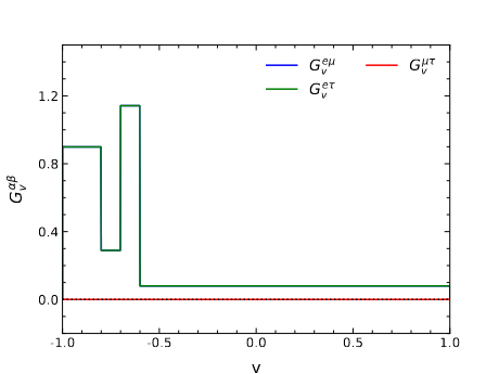
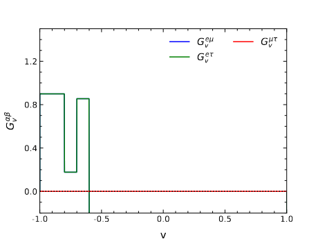
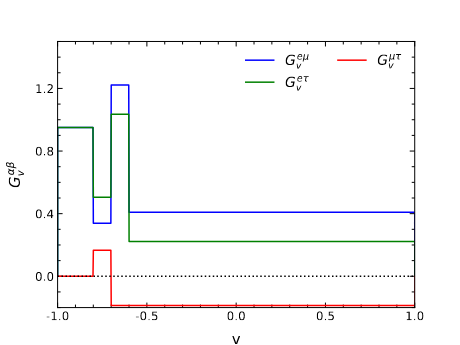
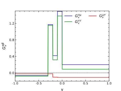
Figure 1: The above panels show the effective lepton numbers for different flavors for the angular distributions of the four toy examples mentioned in the text. The upper left panel corresponds to case 1 and upper right panel is for case 2. The lower left and right panels represent the case 3 and case 4 respectively.

IV Linearized Regime

The onset of the fast flavor conversions is studied through the method of linear stability analysis Izaguirre:2016gsx ; Capozzi:2017gqd ; Yi:2019hrp ; Airen:2018nvp ; Capozzi:2019lso ; Chakraborty:2019wxe . We linearize Eq. 1 at first order in the off-diagonal elements of the density matrices $S_{\textbf{v}}^{\alpha\beta}$, ($\alpha\neq\beta$), assuming the diagonal elements to be $O(1)$ Chakraborty:2019wxe . This leads to the equations

$$i\,v^{\gamma}\partial_{\gamma}S_{\textbf{v}}^{\alpha\beta}=\bigl{(}v^{\gamma}(\Lambda_{\gamma}^{\alpha\beta}+\Phi_{\gamma}^{\alpha\beta})\bigr{)}S_{\textbf{v}}^{\alpha\beta}-v^{\gamma}\int\frac{d\textbf{v}^{\prime}}{4\pi}\,v_{\gamma}^{\prime}\,G_{\textbf{v}^{\prime}}^{\alpha\beta}S_{\textbf{v}^{\prime}}^{\alpha\beta}\,,$$ (10)

where, $\alpha\beta$ corresponds to the three sectors i.e., $e-\mu$, $e-\tau$ and $\mu-\tau$ respectively. Here, $\gamma=0,1,2,3$ and $\Lambda_{\gamma}^{\alpha\beta}$ is the charged lepton matter term and the corresponding current. Similarly, $\Phi_{\gamma}^{\alpha\beta}$ is the neutral lepton matter term and the corresponding current. Since we are neglecting the matter term, we take $\Lambda_{\gamma}^{\alpha\beta}=0$ and $\Phi_{\gamma}^{\alpha\beta}=\int\frac{d\textbf{v}}{4\pi}\,v_{\gamma}\,G_{\textbf{v}}^{\alpha\beta}$.

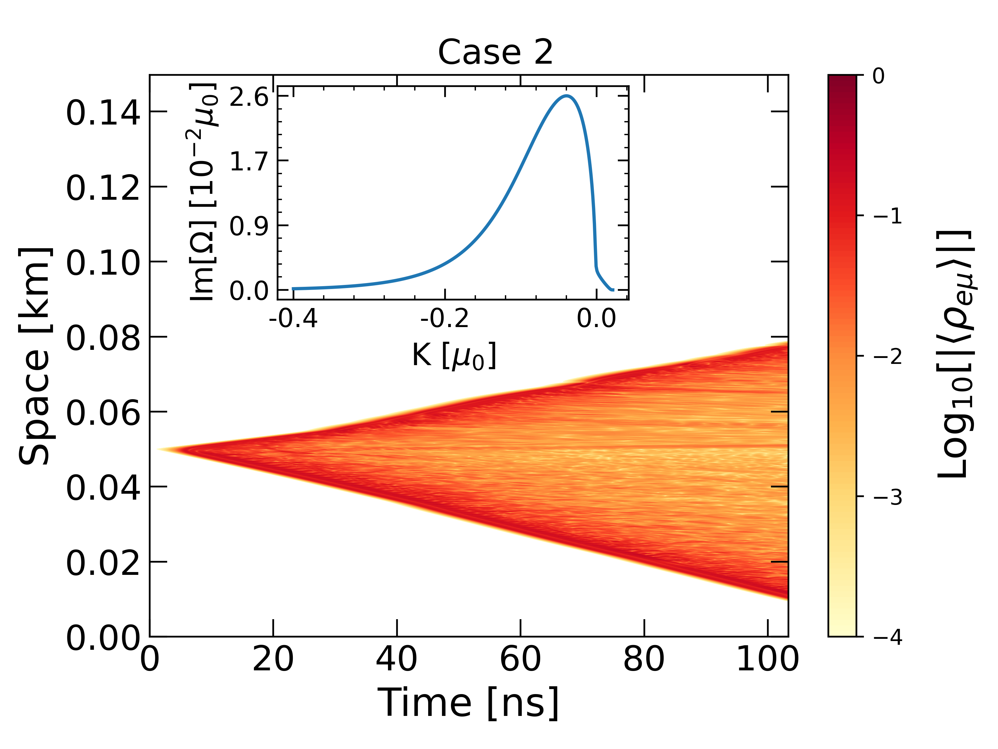
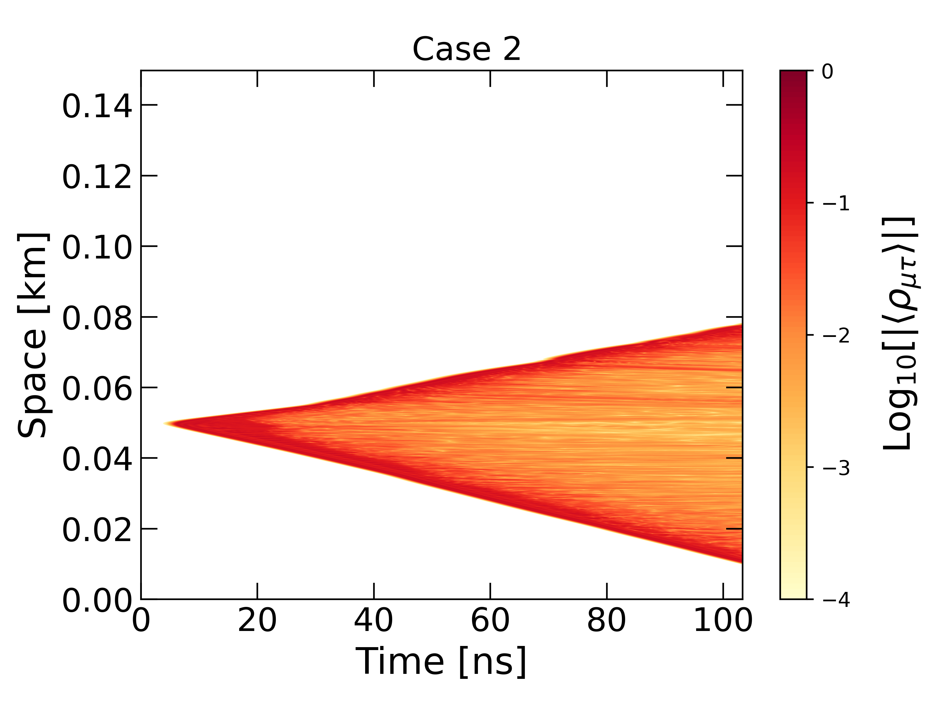
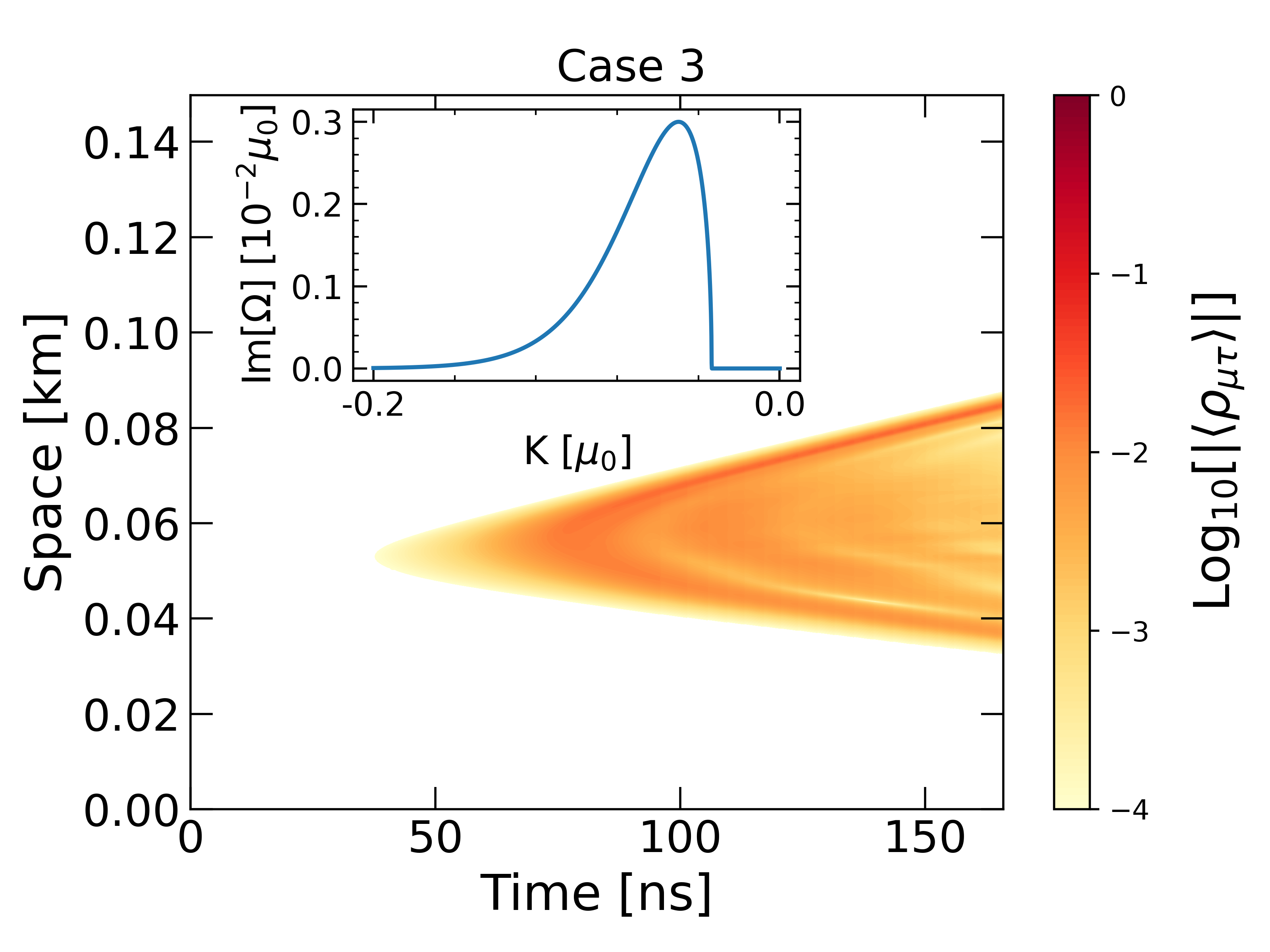
Figure 2: Growth rate of flavor instability $(\log_{10}|\langle\rho_{\alpha\beta}\rangle|)$ in the three-flavor study for the four different cases. The rows (from top to bottom) correspond to cases 1,2,3, and 4, respectively. The left panel depicts the $e-\mu$ sector, while the middle and right panels depict the $e-\tau$ and the $\mu-\tau$ sectors respectively. The inset shows the linear growth rates plotted in units where $\sqrt{2}G_{F}n_{\nu}=1$.

We then take the ansatz $S_{\textbf{v}}^{\alpha\beta}=Q_{\textbf{v}}^{\alpha\beta}\,e^{-i(\Omega t-\textbf{K}\cdot\textbf{x})}$. Substituting this back in Eq. 10, we obtain the dispersion relation for a given choice of $\alpha\beta$,

$${\rm det}\,[\Pi^{\gamma\delta}_{\alpha\beta}(\Omega,K)]=0\,,$$ (11)

where the rank-2 polarization tensor $\Pi^{\gamma\delta}_{\alpha\beta}$ is given by:

$$\Pi^{\gamma\delta}_{\alpha\beta}=\eta^{\gamma\delta}+\int\frac{d\textbf{v}}{4\pi}\,G_{\,\textbf{v}}^{\alpha\beta}\,\frac{v^{\gamma}v^{\delta}}{\Omega-(\textbf{K}-\Phi^{\alpha\beta}).\textbf{v}}\,$$ (12)

where $\eta^{\gamma\delta}$ is the metric tensor and it is equal to diag(+1, -1, -1, -1). Note that the subscripts $\alpha,\beta$ of $\Pi$ denote the flavor of neutrinos and $\gamma,\delta$ are the spacetime indices. Here, there are three dispersion relations corresponding to the three sectors, i.e., $e-\mu$, $e-\tau$ and $\mu-\tau$. To investigate the presence of instabilities in the system, for each sector we solve Eq. 11 as a function of real values of K. If, we find Im$[\Omega(K)]\neq 0$, then we have an instability.

V Full space-time evolution

In this section, we numerically solve the complete equations of motion Eq. 1 in one spatial dimension, $z$ and time $t$ for the four cases discussed above. The results of the simulations allow us to compare the numerical growth rates with those expected from the stability analysis.

For the numerical analysis, we employ the d03pff routine from the NAG library, which is built for solving a system of nonlinear convection-diffusion partial differential equations in one space dimension. The method of lines is employed to reduce the system of partial differential equations to a system of ordinary differential equations, and the resulting system is solved using a backward differentiation formula method. We use this routine with $10^{3}$ points in space and we discretize the angular variable $\mathbf{v}$ with 30 points. We fix $\mu_{0}=4\times 10^{5}$ km^-1 and we consider a spatial range $z\in[0,0.1]$ km. We set H${}_{\rm vac}=0$, but we set the off-diagonal entries of $\rho_{\mathbf{p},z,t=0}$ equal to a Gaussian in space centered at $z=0.05$ km, with an amplitude of $10^{-9}$ and a width of $5\times 10^{-4}$ km. For boundary conditions, we assume that at $t=0$, the density matrix is empty at the edge of our spatial box. This means that neutrinos are only going outside of the box, whereas none is coming in. We use an absolute relative accuracy of $10^{-10}$ up to 30 ns for case 2 and up to 60 ns for cases 3 and 4, then, we switch to $10^{-6}$ in order to speed up calculations. For case 1, we always use $10^{-10}$. We have not imposed a maximum time step.

The results for the four cases, shown in Figure 2, demonstrate the growth rates of flavor instabilities in terms of the evolution of $\log_{10}|\langle\rho_{\alpha\beta}\rangle|$ in the $z-t$ plane, where $\langle\rho_{\alpha\beta}\rangle$ is angle averaged. The leftmost panels depict the evolution in the $e-\mu$ sector, while the middle panels show the same for the $e-\tau$ sector and the $\mu-\tau$ sector respectively. For the cases where we find a flavor instability, we show the corresponding linear growth rate in the inset plot. The growth rates have been obtained by solving the dispersion relation given by Eq. 11 taking into consideration the initial angular distributions of all the flavors.

We find that, as expected, there are no flavor instabilities for case 1 (top panel). This is consistent with the fact that the angular distributions in case 1 show no crossing in three flavors. In tandem with these results, we find null results for the growth rates using a stability analysis. For case 2 (second panel from top), there exists a crossing in the $e-\mu$ and the $e-\tau$ sectors. Consequently, the values of $\log_{10}|\langle\rho_{e\mu}\rangle|$ and $\log_{10}|\langle\rho_{e\tau}\rangle|$ start growing in space and time, indicating a flavor instability. The corresponding inset plots show the instabilities in the Im$\Omega-K$ plane in the linear regime. It can be seen that the instabilities are present for both positive and negative values of $K$. We also get a quantitative agreement among the amplitudes of the growth rates in the linear as well as nonlinear regimes. The growth-rate in the $\mu-\tau$ sector is driven by a combination of the couplings in the different sectors, and is purely driven by the nonlinearity of the problem. Hence, this growth rate is not captured by a stability analysis.

The toy spectra in case 3 (third panel from top) shows a crossing only in the $\mu-\tau$ sector. As a result, we find a flavor instability in the $\mu-\tau$ sector only. The linear stability analysis also obtains imaginary values of $\Omega$ only in the $\mu-\tau$ sector and not in the other two. Furthermore, we note that the instabilities are present only for negative values of $K$.

For case 4 (bottom panel), we find that all three flavor sectors show a nonzero growth of the off-diagonal components of the density matrix. The $e-\mu$ and the $e-\tau$ sectors show a spectral crossing, and hence have a faster growth rate. The growth in the $\mu-\tau$ sector is completely a three-flavor artefact, and does not depend on any spectral crossing in that sector. The same is captured in a linear stability analysis, where there is an instability only in the $e-\mu$ and the $e-\tau$ sector, as shown in the inset. Note that here the instabilities are present only for the positive K.

One interesting thing to note from the linear stability curves (insets of Figure 2) is that in the cases 3 and 4, there are no instabilities for the k = 0 mode. Here, ‘k’ is the shifted wave vector in the corotating frame and is defined as k = K-$\Phi^{\alpha\beta}$, where $\Phi^{\alpha\beta}=\int\frac{d\textbf{v}}{4\pi}\,\textbf{v}\,G_{\textbf{v}}^{\alpha\beta}$ is the neutral lepton current term as defined in Sec. IV. For the given spectra $G_{\textbf{v}}^{\alpha\beta}$ (shown in Figure 1), in case 3, $\Phi^{\mu\tau}$$=-0.00528$ and similarly in case 4, $\Phi^{e\mu}$$=0.00371$ and $\Phi^{e\tau}$$=0.0298$ in units of $\mu_{0}$. From the insets of the lower two panels of Figure 2, one can see that Im($\Omega$) $=0$ corresponding to these values. In other words, no instabilities are present in cases 3 and 4 for K = $\Phi^{\alpha\beta}$, i.e., k = 0 mode. This also agrees with the fact that when we calculate the Im($\Omega$) following the formalism of Ref. Dasgupta:2018ulw by finding the moments, we do not obtain any instability for these cases. This is because the moments formalism is based on the calculation of Im($\Omega$) for the case of k=0. On the other hand, for case 2, $\Phi^{e\mu}=\Phi^{e\tau}$ $=-0.024$, corresponding to which a nonzero Im($\Omega$) exists (shown in the insets of second panel from top of Figure 2), although it is not the maximum value. Therefore, for this case, we obtain instability from the moments calculation.

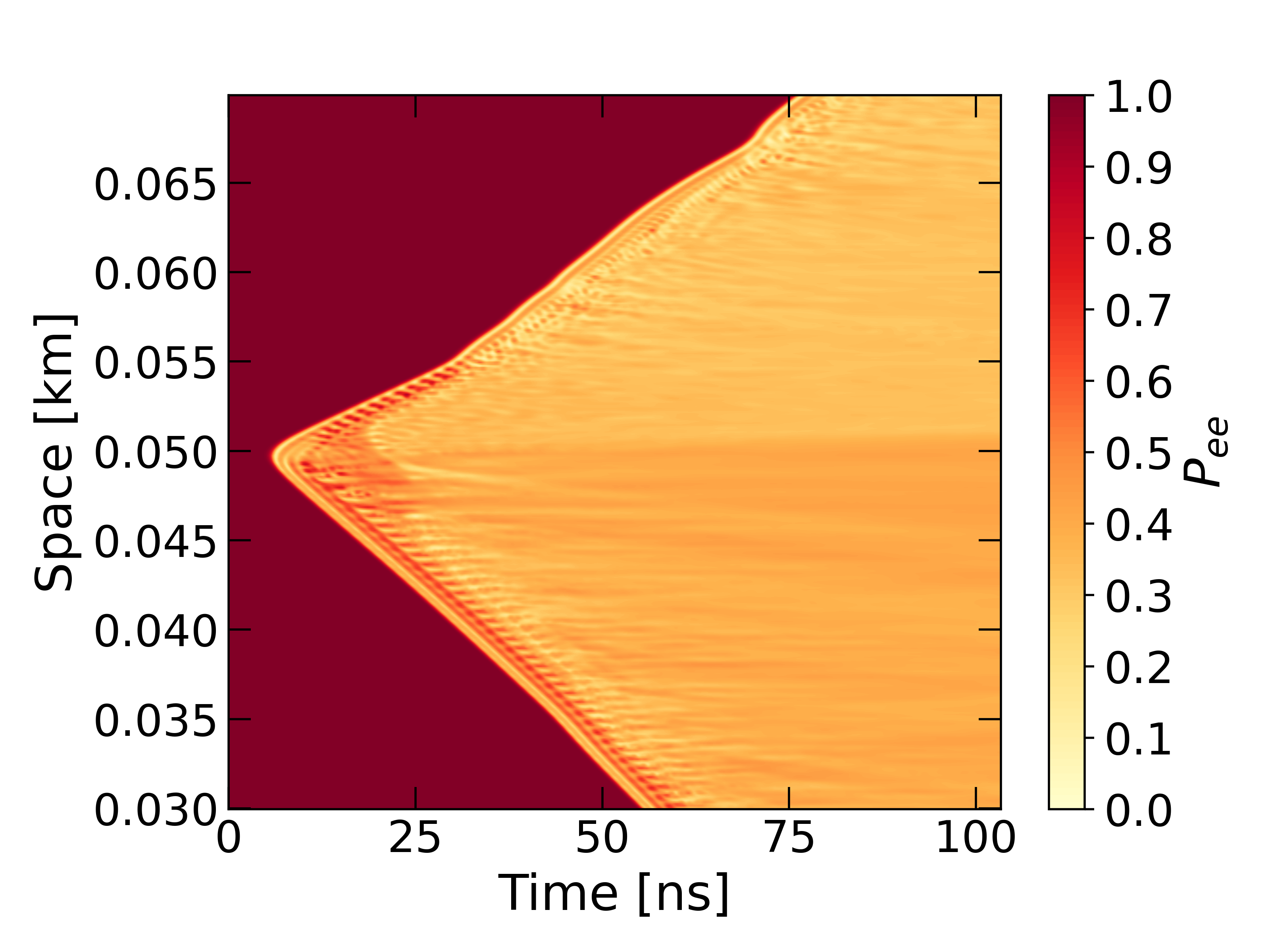
Figure 3: Survival probability $P_{ee}$ obtained with three neutrino species (left panel) and six (right panel). In both panels the flavor evolution is obtained assuming $\rho_{\tau\tau}(z,t=0)=0$ and the same values of $\rho_{ee}(z,t=0)$, $\bar{\rho}_{ee}(z,t=0)$, $\rho_{\mu\mu}(z,t=0)$ and $\bar{\rho}_{\mu\mu}(z,t=0)$ taken from case 2.

VI Two- and three-flavor calculations with the same flavor content

In this section we compare the survival probability $P_{ee}=(\langle\rho_{ee}(t,z)\rangle-\langle\rho_{\mu\mu}(0,z)\rangle)/(\langle\rho_{ee}(0,z)\rangle-\langle\rho_{\mu\mu}(0,z)\rangle)$ between the six and the three neutrino species approach, focusing only on case 2. Note that here $\langle\rho_{\alpha\alpha}\rangle$ is the angle sum. To make a fair comparison, we require that the total number of neutrinos at $t=0$ remains the same in both approaches. Indeed, since flavor evolution of fast conversions is dominated by the self-interaction term, which is proportional to the net neutrino number density, we believe that setting the initial neutrino number density to be the same is the only way to compare three species and six species analyses. As a result, we consider,

$$\rho_{xx}(t=0,z) = \frac{\rho_{\mu\mu}(t=0,z)+\rho_{\tau\tau}(t=0,z)}{2}$$ (13)

$$\bar{\rho}_{xx}(t=0,z) = \frac{\bar{\rho}_{\mu\mu}(t=0,z)+\bar{\rho}_{\tau\tau}(t=0,z)}{2}$$ (14)

Since in a SN-like environment the initial flavor content for the nonelectron flavor neutrinos are approximately equal, the above prescription allows one to compare flavor evolution in the two cases with almost similar initial conditions.

A remark is in order. The choice of initial conditions reported above is different from both what we assumed in our previous work Capozzi:2020kge and from what is considered in Ref. Shalgar:2021wlj . Let us first consider the former case. Here, the two approaches had the same initial flavor content for $\nu_{e}$ and $\bar{\nu}_{e}$. However, the three species approach was used assuming no $\nu_{x}$ at $t=0$, and the six species one had the same initial conditions presented in Figure 1. Such assumptions introduced a difference in the total number of neutrinos between the two approaches. In Ref. Shalgar:2021wlj , the $e$ and $\mu$ flavor content was taken to be the same among the two approaches, but it was imposed $\rho_{\tau\tau}(t=0,z)=\bar{\rho}_{\tau\tau}(t=0,z)=0$. Here, despite having the same number of particles, setting one diagonal entry of the density matrix completely empty can intrinsically enhance the amount of flavor conversions.

Figure 3 shows the survival probability $P_{ee}$ as a function of time and space for the three species case (left panel) and the six species one (right panel). The qualitative natures of the solutions are similar, but we find some differences in the flavor outcome in the two scenarios. Considering $t>25$ ns, in the former case, $P_{ee}\sim 0.5$, while in the latter case, $P_{ee}\sim 0.4$. We emphasize again that a proper quantitative comparison between two- and three-flavor evolution should be performed in a way such that the total numbers of neutrinos are similar in the two cases. Otherwise, if one starts with a scenario where one of the nonelectron flavors, say $\nu_{\tau}$ and $\bar{\nu}_{\tau}$ for example, has a negligible population to start with, a large flavor conversion can be obtained simply because of the lack of entries in the density matrix. This might lead to an enhancement of the differences.

VII Conclusions

The evolution of neutrino fast flavor conversions depends on the occurrence of crossings in the angular distributions of flavor lepton number. In the context of supernova neutrinos, it is usually assumed that the flavor content of $\nu_{\mu}$, $\nu_{\tau}$, $\bar{\nu}_{\mu}$ and $\bar{\nu}_{\tau}$ is equal. Consequently, only three neutrino species are used ($\nu_{e}$, $\bar{\nu}_{e}$ and $\nu_{x}$) in numerical simulations, as well as linear stability analyses. Recently, the first hydrodynamical simulations with six neutrino species Bollig:2017lki were performed. Driven by these, it has been pointed out that the differences expected between $\nu_{\mu}$ and $\bar{\nu}_{\mu}$, which are induced by a non-negligible population of negatively charged muons in the core, can introduce some observable modifications of the angular distributions of lepton number Capozzi:2020kge . As a result, those angular crossings that are expected to occur with three neutrino species can be either erased or actually created. Furthermore, even assuming the same flavor content in both the three and six neutrino species approaches, a significant difference in the survival probabilities is observed Shalgar:2021wlj . However, these conclusions have been obtained considering a spatially homogeneous neutrino system. In this work we have relaxed this assumption and we have performed a numerical calculation in both space and time with six neutrino species.

We have considered the same four cases that we adopted in our previous work Capozzi:2020kge and have solved the complete nonlinear equations of motion in one space and time dimension for each of them. It is evident from Fig. 2 that out of the four cases considered, case 1 does not show any instability as there is no crossing in any of the sectors ($e-\mu$, $e-\tau$, and $\mu-\tau$), while the other three show absolute instabilities. Cases 2 and 4 have instabilities in all the three sectors whereas it is present only in the $\mu-\tau$ sector of case 3. The presence of absolute instability is evident from the fact that in all the cases the instability spreads around the point of origin without drifting. Moreover, the instability propagates in both directions around the origin point (upward and downward). This is because of the backward velocity modes ($v<0$; see Figure 1), which are present in all our numerical examples. The results obtained from the nonlinear analysis are confirmed by the linear one. However, we point out that the triggering of instabilities in the otherwise stable sector $\rho_{\alpha\beta}$, because of the absence of a crossing at $t=0$, can only be observed at the nonlinear level. Overall, we find that the qualitative nature of the results obtained in Ref. Capozzi:2020kge remains robust even when considering flavor evolution in both space and time.

Overall, we find that considering all the six neutrino species can significantly affect the results obtained with only three of them. First, systems that are stable in the standard three species approach can be unstable in the more realistic six species one. Moreover, to make a fair comparison between the two approaches, we have done a numerical analysis starting with same flavor content for both cases, finding a relatively large difference in the flavor outcomes. Thus, this analysis emphasizes the need to include muons in the study of fast flavor conversions and in turn may reveal their influence on the supernova dynamics.

VIII Acknowledgements

The work of F.C. is supported by GVA Grant No.CDEIGENT/2020/003. S.C. acknowledges the support of the Max Planck India Mobility Grant from the Max Planck Society, supporting the visit and stay at MPP during the project. S.C has also received funding from DST/SERB projects CRG/2021/002961 and MTR/2021/000540.

References

- (1) J. T. Pantaleone, Neutrino flavor evolution near a supernova’s core, Phys. Lett. B 342 (1995) 250–256, [astro-ph/9405008].
- (2) H. Duan, G. M. Fuller, and Y.-Z. Qian, Collective neutrino oscillations, Ann. Rev. Nucl. Part. Sci. 60 (2010) 569–594, [1001.2799].
- (3) A. Mirizzi, I. Tamborra, H.-T. Janka, N. Saviano, K. Scholberg, R. Bollig, L. Hüdepohl, and S. Chakraborty, Supernova Neutrinos: Production, Oscillations and Detection, Riv. Nuovo Cim. 39 (2016), no. 1-2 1–112, [1508.00785].
- (4) S. Chakraborty, R. Hansen, I. Izaguirre, and G. G. Raffelt, Collective neutrino flavor conversion: Recent developments, Nucl. Phys. B908 (2016) 366–381, [1602.02766].
- (5) S. Horiuchi and J. P. Kneller, What can be learned from a future supernova neutrino detection?, 1709.01515.
- (6) I. Tamborra and S. Shalgar, New Developments in Flavor Evolution of a Dense Neutrino Gas, Ann. Rev. Nucl. Part. Sci. 71 (2021) 165–188, [2011.01948].
- (7) F. Capozzi and N. Saviano, Neutrino Flavor Conversions in High-Density Astrophysical and Cosmological Environments, Universe 8 (2022), no. 2 94, [2202.02494].
- (8) S. Hannestad, G. G. Raffelt, G. Sigl, and Y. Y. Y. Wong, Self-induced conversion in dense neutrino gases: Pendulum in flavour space, Phys. Rev. D74 (2006) 105010, [astro-ph/0608695]. [Erratum: Phys. Rev.D76,029901(2007)].
- (9) H. Duan, G. M. Fuller, J. Carlson, and Y.-Z. Qian, Analysis of Collective Neutrino Flavor Transformation in Supernovae, Phys. Rev. D 75 (2007) 125005, [astro-ph/0703776].
- (10) G. G. Raffelt, -mode coherence in collective neutrino oscillations, Phys. Rev. D 83 (May, 2011) 105022.
- (11) G. Fogli, E. Lisi, A. Marrone, and A. Mirizzi, Collective neutrino flavor transitions in supernovae and the role of trajectory averaging, Journal of Cosmology and Astroparticle Physics 2007 (dec, 2007) 010–010.
- (12) L. Johns and G. M. Fuller, Strange mechanics of the neutrino flavor pendulum, Phys. Rev. D 97 (2018), no. 2 023020, [1709.00518].
- (13) R. F. Sawyer, Neutrino cloud instabilities just above the neutrino sphere of a supernova, Phys. Rev. Lett. 116 (2016), no. 8 081101, [1509.03323].
- (14) S. Chakraborty, R. S. Hansen, I. Izaguirre, and G. G. Raffelt, Self-induced neutrino flavor conversion without flavor mixing, JCAP 1603 (2016), no. 03 042, [1602.00698].
- (15) B. Dasgupta, A. Mirizzi, and M. Sen, Fast neutrino flavor conversions near the supernova core with realistic flavor-dependent angular distributions, JCAP 1702 (2017), no. 02 019, [1609.00528].
- (16) S. Airen, F. Capozzi, S. Chakraborty, B. Dasgupta, G. Raffelt, and T. Stirner, Normal-mode Analysis for Collective Neutrino Oscillations, JCAP 12 (2018) 019, [1809.09137].
- (17) I. Izaguirre, G. G. Raffelt, and I. Tamborra, Fast Pairwise Conversion of Supernova Neutrinos: A Dispersion-Relation Approach, Phys. Rev. Lett. 118 (2017), no. 2 021101, [1610.01612].
- (18) X. Li and D. M. Siegel, Neutrino Fast Flavor Conversions in Neutron-Star Postmerger Accretion Disks, Phys. Rev. Lett. 126 (2021), no. 25 251101, [2103.02616].
- (19) I. Padilla-Gay, I. Tamborra, and G. G. Raffelt, Neutrino Flavor Pendulum Reloaded: The Case of Fast Pairwise Conversion, Phys. Rev. Lett. 128 (2022), no. 12 121102, [2109.14627].
- (20) M.-R. Wu, M. George, C.-Y. Lin, and Z. Xiong, Collective fast neutrino flavor conversions in a 1D box: Initial conditions and long-term evolution, Phys. Rev. D 104 (2021), no. 10 103003, [2108.09886].
- (21) S. Richers, D. E. Willcox, N. M. Ford, and A. Myers, Particle-in-cell Simulation of the Neutrino Fast Flavor Instability, Phys. Rev. D 103 (2021), no. 8 083013, [2101.02745].
- (22) S. Richers, D. Willcox, and N. Ford, Neutrino fast flavor instability in three dimensions, Phys. Rev. D 104 (2021), no. 10 103023, [2109.08631].
- (23) J. D. Martin, C. Yi, and H. Duan, Dynamic fast flavor oscillation waves in dense neutrino gases, Phys. Lett. B 800 (2020) 135088, [1909.05225].
- (24) S. Abbar and M. C. Volpe, On Fast Neutrino Flavor Conversion Modes in the Nonlinear Regime, Phys. Lett. B790 (2019) 545–550, [1811.04215].
- (25) L. Johns, H. Nagakura, G. M. Fuller, and A. Burrows, Fast oscillations, collisionless relaxation, and spurious evolution of supernova neutrino flavor, Phys. Rev. D 102 (2020), no. 10 103017, [2009.09024].
- (26) G. Sigl, Simulations of fast neutrino flavor conversions with interactions in inhomogeneous media, Phys. Rev. D 105 (2022), no. 4 043005, [2109.00091].
- (27) Z. Xiong and Y.-Z. Qian, Stationary solutions for fast flavor oscillations of a homogeneous dense neutrino gas, Phys. Lett. B 820 (2021) 136550, [2104.05618].
- (28) S. Abbar and F. Capozzi, Suppression of fast neutrino flavor conversions occurring at large distances in core-collapse supernovae, JCAP 03 (2022), no. 03 051, [2111.14880].
- (29) M. Delfan Azari, S. Yamada, T. Morinaga, H. Nagakura, S. Furusawa, A. Harada, H. Okawa, W. Iwakami, and K. Sumiyoshi, Fast collective neutrino oscillations inside the neutrino sphere in core-collapse supernovae, Phys. Rev. D 101 (2020), no. 2 023018, [1910.06176].
- (30) H. Nagakura, T. Morinaga, C. Kato, and S. Yamada, Fast-pairwise collective neutrino oscillations associated with asymmetric neutrino emissions in core-collapse supernova, 1910.04288.
- (31) H. Nagakura and L. Johns, New method for detecting fast neutrino flavor conversions in core-collapse supernova models with two-moment neutrino transport, Phys. Rev. D 104 (2021), no. 6 063014, [2106.02650].
- (32) S. Abbar, Searching for Fast Neutrino Flavor Conversion Modes in Core-collapse Supernova Simulations, JCAP 05 (2020) 027, [2003.00969].
- (33) H. Nagakura, L. Johns, A. Burrows, and G. M. Fuller, Where, when, and why: Occurrence of fast-pairwise collective neutrino oscillation in three-dimensional core-collapse supernova models, Phys. Rev. D 104 (2021), no. 8 083025, [2108.07281].
- (34) C. J. Stapleford, C. Fröhlich, and J. P. Kneller, Coupling Neutrino Oscillations and Simulations of Core-Collapse Supernovae, Phys. Rev. D 102 (2020), no. 8 081301, [1910.04172].
- (35) F. Capozzi, B. Dasgupta, and A. Mirizzi, Model-independent diagnostic of self-induced spectral equalization versus ordinary matter effects in supernova neutrinos, Phys. Rev. D 98 (2018), no. 6 063013, [1807.00840].
- (36) M.-R. Wu, I. Tamborra, O. Just, and H.-T. Janka, Imprints of neutrino-pair flavor conversions on nucleosynthesis in ejecta from neutron-star merger remnants, Phys. Rev. D 96 (2017), no. 12 123015, [1711.00477].
- (37) M. Zaizen, J. F. Cherry, T. Takiwaki, S. Horiuchi, K. Kotake, H. Umeda, and T. Yoshida, Neutrino halo effect on collective neutrino oscillation in iron core-collapse supernova model of a 9.6 star, JCAP 06 (2020) 011, [1908.10594].
- (38) G. G. Raffelt and G. Sigl, Self-induced decoherence in dense neutrino gases, Phys. Rev. D 75 (2007) 083002, [hep-ph/0701182].
- (39) A. Esteban-Pretel, S. Pastor, R. Tomas, G. G. Raffelt, and G. Sigl, Decoherence in supernova neutrino transformations suppressed by deleptonization, Phys. Rev. D 76 (2007) 125018, [0706.2498].
- (40) H. Duan, G. M. Fuller, and Y.-Z. Qian, Collective neutrino flavor transformation in supernovae, Phys. Rev. D 74 (2006) 123004, [astro-ph/0511275].
- (41) R. F. Sawyer, Speed-up of neutrino transformations in a supernova environment, Phys. Rev. D72 (2005) 045003, [hep-ph/0503013].
- (42) R. F. Sawyer, The multi-angle instability in dense neutrino systems, Phys. Rev. D79 (2009) 105003, [0803.4319].
- (43) F. Capozzi, B. Dasgupta, E. Lisi, A. Marrone, and A. Mirizzi, Fast flavor conversions of supernova neutrinos: Classifying instabilities via dispersion relations, Phys. Rev. D96 (2017), no. 4 043016, [1706.03360].
- (44) A. Dighe and M. Sen, Nonstandard neutrino self-interactions in a supernova and fast flavor conversions, Phys. Rev. D97 (2018), no. 4 043011, [1709.06858].
- (45) B. Dasgupta and M. Sen, Fast Neutrino Flavor Conversion as Oscillations in a Quartic Potential, Phys. Rev. D97 (2018), no. 2 023017, [1709.08671].
- (46) B. Dasgupta, A. Mirizzi, and M. Sen, Simple method of diagnosing fast flavor conversions of supernova neutrinos, Phys. Rev. D98 (2018), no. 10 103001, [1807.03322].
- (47) S. Abbar, H. Duan, K. Sumiyoshi, T. Takiwaki, and M. C. Volpe, On the occurrence of fast neutrino flavor conversions in multidimensional supernova models, 1812.06883.
- (48) M. D. Azari, S. Yamada, T. Morinaga, W. Iwakami, H. Nagakura, and K. Sumiyoshi, Linear Analysis of Fast-Pairwise Collective Neutrino Oscillations in Core-Collapse Supernovae based on the Results of Boltzmann Simulations, 1902.07467.
- (49) L. Johns, H. Nagakura, G. M. Fuller, and A. Burrows, Neutrino oscillations in supernovae: angular moments and fast instabilities, Phys. Rev. D 101 (2020), no. 4 043009, [1910.05682].
- (50) R. Glas, H. T. Janka, F. Capozzi, M. Sen, B. Dasgupta, A. Mirizzi, and G. Sigl, Fast Neutrino Flavor Instability in the Neutron-star Convection Layer of Three-dimensional Supernova Models, Phys. Rev. D 101 (2020), no. 6 063001, [1912.00274].
- (51) S. Shalgar, I. Padilla-Gay, and I. Tamborra, Neutrino propagation hinders fast pairwise flavor conversions, 1911.09110.
- (52) S. Bhattacharyya and B. Dasgupta, Fast Neutrino Flavor Conversion at Late Time, 2005.00459.
- (53) S. Bhattacharyya and B. Dasgupta, Fast Flavor Depolarization of Supernova Neutrinos, Phys. Rev. Lett. 126 (2021), no. 6 061302, [2009.03337].
- (54) S. Bhattacharyya and B. Dasgupta, Fast flavor oscillations of astrophysical neutrinos with 1, 2, …, crossings, JCAP 07 (2021) 023, [2101.01226].
- (55) T. Morinaga, Fast neutrino flavor instability and neutrino flavor lepton number crossings, 2103.15267.
- (56) B. Dasgupta, Collective Neutrino Flavor Instability Requires a Crossing, Phys. Rev. Lett. 128 (2022), no. 8 081102, [2110.00192].
- (57) S. Bhattacharyya and B. Dasgupta, Elaborating the Ultimate Fate of Fast Collective Neutrino Flavor Oscillations, 2205.05129.
- (58) M. Zaizen and T. Morinaga, Nonlinear evolution of fast neutrino flavor conversion in the preshock region of core-collapse supernovae, Phys. Rev. D 104 (2021), no. 8 083035, [2104.10532].
- (59) M. Chakraborty and S. Chakraborty, Three flavor neutrino conversions in supernovae: slow & fast instabilities, JCAP 2001 (2020), no. 01 005, [1909.10420].
- (60) F. Capozzi, M. Chakraborty, S. Chakraborty, and M. Sen, Fast flavor conversions in supernovae: the rise of mu-tau neutrinos, Phys. Rev. Lett. 125 (2020) 251801, [2005.14204].
- (61) S. Shalgar and I. Tamborra, Three flavor revolution in fast pairwise neutrino conversion, Phys. Rev. D 104 (2021), no. 2 023011, [2103.12743].
- (62) G. Sigl and G. G. Raffelt, General kinetic description of relativistic mixed neutrinos, Nucl. Phys. B406 (1993) 423–451.
- (63) S. Abbar and H. Duan, Fast neutrino flavor conversion: roles of dense matter and spectrum crossing, 1712.07013v1.
- (64) R. Bollig, H. T. Janka, A. Lohs, G. Martinez-Pinedo, C. J. Horowitz, and T. Melson, Muon Creation in Supernova Matter Facilitates Neutrino-driven Explosions, Phys. Rev. Lett. 119 (2017), no. 24 242702, [1706.04630].
- (65) C. Yi, L. Ma, J. D. Martin, and H. Duan, The dispersion relation of the fast neutrino oscillation wave, 1901.01546.
- (66) F. Capozzi, G. Raffelt, and T. Stirner, Fast Neutrino Flavor Conversion: Collective Motion vs. Decoherence, JCAP 09 (2019) 002, [1906.08794].