The Quadruple Image Configurations of Asymptotically Circular Gravitational Lenses

Abstract

The quadruple image configurations of gravitational lenses with vanishing ellipticity are examined. Even though such lenses asymptotically approach circularity, the configurations are stable if the position of the source relative to the vanishing diamond caustic is held constant. The configurations are the solutions of a quartic equation, an “Asymptotically Circular Lens Equation” (ACLE), parameterized by a single complex quantity. Several alternative parameterizations are examined. Relative magnifications of the images are derived. When a non-vanishing quadrupole, in the form of an external shear (XS), is added to the singular isothermal sphere (SIS), its configurations emerge naturally as stretched and squeezed versions of the circular configurations. And as the SIS+XS model is a good first approximation for most quadruply lensed quasars, their configurations likewise have only $2+1$ salient dimensions. The asymptotically circular configurations can easily be adapted to the problem of Solar System “occultation flashes.”

1 Introduction

The simplest models for quadruply lensed quasars (henceforth quads) require seven parameters. Four of these are relatively uninteresting, governing position, angular orientation on the sky, and an overall scale. The interesting variations among different quads are due to the three remaining degrees of freedom. These three are straightforwardly parameterized by the $x$ and $y$ coordinates of the displacement of the source from the line of sight to the center of the potential and the amplitude of the potential’s quadrupole term.

In the present paper, we further simplify the problem by analyzing the quads formed by an asymptotically circular lens, reducing the number of salient parameters to two. This two dimensional model space can be described solely by the relative position of the source with respect to the center of the potential.

Lens experts might reflexively object that, as the ellipticity of a potential approaches zero its “diamond caustic” – inside which the source must lie to produce four images (Ohanian, 1983) – must also vanish. But if we correspondingly scale the distance of the source from the center of the lens, keeping its position relative to the diamond caustic constant, we get a stable configuration of four images on a circle.

The quadruple configurations of the vanishingly elliptical lens can be (and have been) found in a variety of seemingly different contexts. But the connections among these multiple resurfacings have been hidden by different parameterizations, different labeling conventions and different emphases.

Here we describe three distinct parameterizations for these configurations, two of which are in terms of model parameters and one of which is in terms of observable quantities.

We begin, in Section 2, with the Witt-Wynne geometric solution of the lens equation for the singular isothermal elliptical potential (SIEP) of Schechter & Wynne (2019), not because of chronological precedence but because it displays the solutions graphically.

The circular Witt-Wynne construction can be solved algebraically, yielding a quartic equation for the polar angles of the four images. We call this the “Asymptotically Circular Lens Equation” (henceforth ACLE). It reappears in subsequent sections and serves to establish the connection between superficially different circumstances. Woldesenbet & Williams (2012) give closed form solutions for the four images in their discussion of the singular isothermal quadrupole potential (henceforth SIQP).

This quartic equation was first derived by Kassiola & Kovner (1995) in their discussion of the lens equation for the SIQP, which we review in Section 3. Their polar angles, measured with respect to the center of the lens potential, are independent of the strength of the quadrupole, but they do not explicitly address the asymptotically circular case. Kassiola and Kovner isolated a relation among the four angles, their “configuration invariant”, that in effect establishes the two dimensionality of the solution subspace.

For both the vanishingly elliptical SIEP and the SIQP, the space for which the ACLE yields four distinct solutions is bounded by an astroid. In Section 4 we introduce a new coordinate system in which the radial distance from the origin is measured as a fraction of the distance to that astroid.

The parameterizations of the quadruple configurations of asymptotically circular lenses are not limited to using model quantities. Woldesenbet & Williams (2012) showed that the angular solution space of the SIQP could be completely described in terms of two differences of the observed angular coordinates of its images. This yielded a two dimensional “Fundamental Surface of Quads” (henceforth FSQ). We derive it from the ACLE in Section 5. The great majority of quadruply lensed quasars lie close to this surface despite the fact that their potentials are non-circular and better fit by models other than the SIQP.

In Section 6 we reintroduce the third dimension by examining the singular isothermal sphere with external shear (SIS+XS). We show that for the same relative source position within the diamond caustic, the configurations with shear are simply “scronched” versions of the circular configurations. In Section 7, we revisit the SIEP allowing for non-vanishing ellipticity.

Though he does not explore image configurations, An (2005) shows that the two dimensional solution space of the ACLE is not restricted to isothermal potentials and applies more generally to non-isothermal potentials with vanishing quadrupoles. Saha & Williams (2003) had previously noted that

“…properties that arise because of the breaking of circular symmetry are relatively model independent and robustly reproduced by even a rudimentary model.”

In Section 8 we arrive at the same conclusion by an alternative and perhaps more straightforward route, considering the case of circularly symmetric potentials with vanishing external shear.

The ACLE is of use even beyond gravitational lensing. In Section 9 we consider the quadruple image configurations calculated for a “central flash” observed during a 1989 occultation by Saturn (Nicholson et al., 1995). We find they lie closer to the FSQ than do the observed configurations of known quadruply lensed quasars.

In Section 10 we discuss the relative flux ratios for the ACLE quadruple image configurations.

2 Quadruple Configurations of the Asymptotically Circular Lens from the Witt-Wynne construction

Figure 1: The plots show the construction of several asymptotically circular image configurations. Panel (b) shows a “kite” configuration, symmetric around one of the two diagonals connecting the images. The system in panel (c) can be thought of as a “super-kite”, symmetric around both diagonals. The system in panel (a) is symmetric about neither diagonal, and hence an “un-kite.”

Schechter & Wynne (2019) present a simple geometric construction that gives 4 images for an SIEP. Their ‘recipe’ proceeds as follows:

“(1) Find the rectangular hyperbola that passes through the points. (2) Find the aligned ellipse that also passes through them. (3) Find the hyperbola with asymptotes parallel to those of the first that passes through the center of the ellipse and the pair of images closest to each other.”

The center of the ellipse gives the position of the source, and the asymptotes of the hyperbola are aligned with the major and minor axes of the potential. The ellipse has the same axis ratio as the potential, but lies perpendicular to it.

Nothing in the above recipe requires that the ellipse have non-zero ellipticity. For an SIEP of vanishing ellipticity, Wynne’s ellipse becomes a circle. This suggests that by inverting the Witt-Wynne construction, we can use its limiting cases to produce the quadruple configurations formed by asymptotically circular isothermal potentials.

2.1 Edge case of the Witt-Wynne recipe

We invert the Schechter & Wynne (2019) recipe as follows:

1. Start with a unit circle, the limiting case of Wynne’s ellipse (Wynne & Schechter, 2018).

2. Draw a rectangular hyperbola with arbitrary semi-major axis, whose asymptotes (with no loss of generality) are parallel to the $x$- and $y$-axes and one of whose branches passes through the center of the circle. This is our Witt hyperbola (Witt, 1996).

3. The points of intersections of these two conic sections give the positions of the images of a quadruply lensed quasar.

The $x$ and $y$ axes are the symmetry axes of the SIEP by virtue of having constructed the asymptotes of the hyperbola parallel to them.

Figure 1 shows some examples with the associated circle and hyperbola for three different configurations. To qualitatively describe the quads, we use the classification system of Saha & Williams (2003). Figure 1(a) is an example of the “inclined quad” configuration, where the source lies on neither axis of the diamond caustic. Figure 1(b), where the source lies on either axis of the diamond caustic, would form a “long” or “short axis quad”, if the potential were not circular. Figure 1(c) shows a “core” configuration, where the source lies almost at the center of the diamond caustic. The center of the potential is displaced infinitesimally from the source.

2.2 Two-dimensionality of the asymptotically circular model space of Witt-Wynne configurations

Recall that we are not concerned about the scale, rotation, or absolute position of configurations, so we can neglect the orientation and position of the chosen random rectangular hyperbola and the size of the circle. The only two degrees of freedom are the ratio of the major axis of the hyperbola to that of the radius of the circle and the position of the center of the circle on the rectangular hyperbola, characterized by one parameter each. Hence, the configurations generated in the circular limit of Witt-Wynne method are two-dimensional.

2.3 The Asymptotically Circular Lens Equation

The image configurations of a circular potential are described by the four angles $\theta$ around the circle. In Appendix A we show that for Witt’s hyperbola centered at $(x_{h},y_{h})$ and a Wynne circle of radius $b$ centered at the origin, the four angles are the solution of

$$e^{4i(\theta-\psi)}-2We^{3i(\theta-\psi)}+2\overline{W}e^{i(\theta-\psi)}-1=0,$$ (1)

where

$$W=\frac{x_{h}+iy_{h}}{b}.$$ (2)

Equation (1) has exactly the same form, up to multiplicative constants, as equation (2.4) of Kassiola and Kovner, who derived it for solutions of the SIQP potential with finite quadrupole, which we discuss in Section 3. But it is applicable far beyond, so we refer to it as the “Asymptotically Circular Lens Equation” (ACLE). We show in Section 8 that the ACLE, while derived using singular isothermal potentials, gives solutions for all nearly circular potentials with vanishing quadrupole.

The parameter $\psi$ (the position angle of one of the two symmetry axes) merely rotates the configuration. The roots of the ACLE, $\theta_{1},\theta_{2},\theta_{3},$ and $\theta_{4}$, are the angular positions of the four images. Applying Vieta’s formula, we have

$$\psi=\frac{\theta_{1}+\theta_{2}+\theta_{3}+\theta_{4}}{4}\pm\frac{\pi}{4}$$ (3)

a result that also traces back at least as far as Kassiola & Kovner (1995).

Woldesenbet & Williams (2012) give closed form expressions for the four solutions to the ACLE. In Appendix B we recast the closed form solution retaining the original complex parameters $W$ and $\overline{W}$. The four solutions are given by a single equation,

$$2e^{i\theta} = W\widehat{\pm}\sqrt{u+W^{2}}$$

$$\widetilde{\pm} \sqrt{(W\widehat{\pm}\sqrt{u+W^{2}})^{2}-2\left(u\widehat{\pm}\sqrt{u^{2}+4}\right)}$$

with a solution for each pair of choices of $\widehat{\pm}$ and $\widetilde{\pm}$, and where complex $u$ is the solution to the cubic

$$u^{3}+4(1-W\overline{W})u+4(W^{2}-\overline{W}^{2})=0$$ (5)

The solutions to the ACLE are governed entirely by a single complex number. The space of quadruple configurations for lenses of vanishing ellipticity is again seen to be two dimensional.

We show in Appendix A that if Equation (1) has four distinct solutions for $\theta$, $W$ must lie inside a unit astroid. Adopting a coordinate system with $\psi=0$, the astroid is aligned with its axes,

$$W=p+iq,\qquad p,q\in\mathbb{R}$$ (6)

$$p^{2/3}+q^{2/3}<1.$$ (7)

In this aligned coordinate system, the ACLE takes on the deceptively simple form

$$p\sec\theta+q\csc\theta=1\quad.$$ (8)

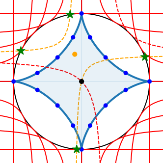
Figure 2: The blue dots are the centers of the Witt’s hyperbolae (red), which are drawn tangent to the Wynne’s circle (black). A configuration (green stars) is constructed for an arbitrary position of center of Witt’s hyperbola (yellow) to illustrate how configurations are generated from points inside the Witt-Wynne diamond.

2.4 Hyperbolae tangent to the Wynne circle and the astroid formed by their centers

In the Witt-Wynne construction, the image configurations are determined solely by the position of the center of Witt’s hyperbola, $W$. The hyperbola is constrained to pass through the center of Wynne’s circle (which coincides with the source position). One can construct the astroid that bounds the four image solutions by plotting the centers of the hyperbolae tangential to the circle.

Two images (e)merge and (dis)appear at the point of tangency. The centers of the tangent hyperbolae demarcate the envelope of the four image region. Figure 2 shows how these centers trace the astroid inside which Witt’s hyperbola gives four images.

Using this same construction for an SIEP with finite ellipticity, one obtains a scronched astroid, the discussion of which we defer until Section 6. In Section 5 we discuss the Witt-Wynne construction for SIS+XS potentials, which likewise give scronched astroids.

The “Witt-Wynne diamonds,” traced by the center of Wynne’s hyperbola, should not be mistaken for Ohanian’s (1983) diamond caustics, traced by the source position (although they are clearly related). In general the diameters of those diamond caustics are not equal. For both the SIEP and an SIS+XS, the diamond caustic is elongated perpendicular to the elongation of the Witt-Wynne diamond. The center of the hyperbola and the source lie in different quadrants of the complex plane. And for the case of the SIEP, the diamond caustic differs, albeit subtly, from a scronched astroid.

2.5 The center of Witt’s hyperbola from the average image position

The center of Witt’s hyperbola can be found by expressing it as a conic section, with four unknown coefficients, evaluating it at each of the four images and solving for coefficients by inverting a $4\times 4$ matrix. Alternatively, we show in Appendix A that $(x_{h},y_{h})$, the coordinates of the center of Witt’s hyperbola relative to the center of Wynne’s circle can be calculated from the coordinates of the centroid of the four images and are given by $2(x_{\textrm{\scriptsize centroid}},y_{\textrm{\scriptsize centroid}})$.

3 The ACLE derived from the not-at-all circular SIQP

In the previous section, we constructed geometrically the angular configurations generated by an asymptotically circular singular isothermal potential. Identical angular configurations arise for the singular isothermal quadrupole potential, even when the amplitude of the quadrupole is far from vanishing. The configurations differ, however, in that the radial deflections vary with angle. The properties of the SIQP have been extensively studied in the literature (Kochanek, 1991), (Kassiola & Kovner, 1995), (Kormann et al., 1994) and (Dalal, 1998), but without taking note of the limiting circular case.

3.1 Configurations of the SIQP and equivalence to those of the ACLE

We consider the singular isothermal quadrupole potential (SIQP),

$$\Phi(r,\theta)=br[1-\epsilon\cos{2(\theta-\psi)}]$$ (9)

Here $\psi$ is the position angle of the major axis of the quadrupole of the SIQP and $\epsilon$ is proportional to the quadrupole moment.

Starting with the angular component of the lens equation Kassiola & Kovner (1995) derived an equation for the image positions that is identical, modulo multiplicative constants, to our Equation (1), the ACLE. Treating the position of the source relative to the potential as a complex number

$$s=re^{i(\phi_{s}-\psi)}\quad,$$ (10)

taking $\psi$ to be the position angle of the major axis and $\theta$ to be the angular position of an image measured from the center of the lens. Kassiola & Kovner (1995)’s polynomial equation (2.4) for the positions of the images can be rewritten as

$$e^{4i(\theta-\psi)}-\frac{\bar{s}}{2\epsilon b}e^{3i(\theta-\psi)}+\frac{s}{2\epsilon b}e^{i(\theta-\psi)}-1=0.$$ (11)

This becomes identical to Equation (1), the asymptotically circular lens equation, if we take

$$W=\frac{\bar{s}}{4\epsilon b}\quad.$$ (12)

All finite amplitudes of the quadrupole in the range $-\frac{1}{5}\leq\epsilon\leq\frac{1}{5}$ (Finch et al., 2002), including a fortiori the asymptotically circular case when $\epsilon\rightarrow 0$, give the same set of four image angular configurations.

It is reassuring that angular configurations for the asymptotically circular SIQP are the same as those for the asymptotically circular SIEP of Section 2. But note that for the SIEP, the complex quantity $W$ in the ACLE is defined, in Equation (2), in terms of the position of the center of Witt’s hyperbola, while for the SIQP, it is defined in terms of the position of the source. As with the SIEP, the SIQP gives four images if $W$ lies within a unit astroid.

Kormann et al. (1994, eq. 49), tell us that for a potential aligned with one of the axes, the diamond caustic of the SIQP has coordinates $(x_{a},y_{a})$ given by

$$x_{a}=~{}4\epsilon b\cos^{3}\theta_{c},$$

$$y_{a}=-4\epsilon b\sin^{3}\theta_{c}.$$ (13)

where $\theta_{c}$ is the angular position at which two images merge on the critical curve. For the SIQP the diamond caustic is therefore a true astroid with the equation,

$$\left(\frac{x_{a}}{4\epsilon b}\right)^{2/3}+\left(\frac{y_{a}}{4\epsilon b}\right)^{2/3}=1.$$ (14)

But since four image solutions to the ACLE must lie within an astroid, we might also have arrived at this result using equations (6) and (7). The angular image configurations for the SIQP, therefore depend only upon the position of the source relative to the center of the potential, $s$, scaled by the size of the astroidal caustic. In Section 4, we explore how the configurations vary as the source position varies within the astroid.

3.2 The Kassiola-Kovner Invariant

The coefficient of the $e^{2i\theta}$ term in the ACLE vanishes. We show in Appendix C that if $\theta_{1},\theta_{2},\theta_{3},$ and $\theta_{4}$ are distinct roots of the ACLE, then the following identity holds

$$\cos\frac{\theta_{1}+\theta_{2}-\theta_{3}-\theta_{4}}{2}+\cos\frac{\theta_{1}+\theta_{3}-\theta_{2}-\theta_{4}}{2}$$

$$+\cos\frac{\theta_{1}+\theta_{4}-\theta_{2}-\theta_{3}}{2}=0.\quad\quad$$ (15)

This invariant of the SIQP was discovered by Kassiola & Kovner (1995), who called it the “configuration invariant”. But beyond the SIQP, the Kassiola and Kovner invariant is exactly $0$ for any lens satisfying the ACLE. Moreover, its invariance holds approximately for many known lenses (Kassiola & Kovner, 1995). In Section 4 we explore its connection to the “Fundamental Surface of Quads” (FSQ), found independently by Woldesenbet & Williams (2012).

4 Parameterizing asymptotically circular lens configurations with observed angular differences

In the preceding sections we use the model parameters of the asymptotically circular lens to describe the two dimensional space of quadruple image configurations. Here we examine the configurations’ three observed angular differences, which Woldesenbet and Williams have shown lie on a two dimensional surface, the FSQ. Any two of the observed differences can be used to derive the third.

4.1 Labeling convention

The three angular differences used by Woldesenbet and Williams are not interchangeable. They label their images so that photons arrive first from image #1 and last from image #4, as shown in Figure 3.

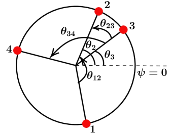
Figure 3: For consistency with the notation of Woldesenbet & Williams (2012), we label the images as shown in this figure. Images $2$ and $3$ are the closest pair of images. The quadrant in which they lie depends upon the angular position of the source relative to the lens, $\phi_{s}$. For the configuration shown, $\phi_{s}$ lies in the $4^{\textrm{\scriptsize th}}$ quadrant

They define angular differences as follows:

$$\theta_{12} =\pm(\theta_{2}-\theta_{1}),$$

$$\theta_{23} =\mp(\theta_{3}-\theta_{2}),$$

$$\theta_{34} =\pm(\theta_{4}-\theta_{3}),$$ (16)

where $\pm$ is $+$ when the source position, $\phi_{s}$, is in $2^{\textrm{\scriptsize nd}}$ or $4^{\textrm{\scriptsize th}}$ quadrant and $-$ when $\phi_{s}$ in $1^{\textrm{\scriptsize st}}$ or $3^{\textrm{\scriptsize rd}}$ quadrant. Note that $\theta_{23}$, the angular difference between the two closest images, is defined oppositely from the other two. Its modulus is always less than $90^{\circ}$. The directions in which the differences are measured are shown in Figure 3.

Figure 4: The two plots compare the Fundamental Surface of Quads (FSQ) (orange) and the surface corresponding to the configuration invariant (blue). Panel (a) shows the FSQ and the surface of configuration invariant superimposed on each other, restricted to $\theta_{23}>0$. Panel (b) shows the difference between the FSQ and the configuration invariant. The blue is the zero plane and orange denotes the difference function. Note the different scales on the vertical axes. The planar axes are the same for both panels, while the vertical axes are $\theta_{23}$ and $\Delta\theta_{23}$, respectively.

4.2 The Fundamental Surface of Quads

Woldesenbet & Williams (2012) discovered a quasi-two-dimensionality of the space of quadruple lenses. They used the closed form solutions for the four image positions, $\theta_{i}$, of the SIQP (which they call SISell) and after taking differences, plotted them on the basis $(\theta_{23},\theta_{12},\theta_{34})$. They found a “nearly invariant two-dimensional surface” – the Fundamental Surface of Quads – to which they fitted a polynomial

$$\theta_{23} = -5.792+1.783\>\theta_{12}+1.784\>\theta_{34}$$ (17)

$$+ 0.1648\>\theta_{12}^{2}+0.1643\>\theta_{34}^{2}-0.7275\>\theta_{12}\theta_{34}$$

$$- 0.04591\>\theta_{12}^{3}-0.04579\>\theta_{34}^{3}$$

$$+ 0.0549\>\theta_{12}^{2}\theta_{34}+0.05493\>\theta_{12}\theta_{34}^{2}$$

$$- 0.0001486\>\theta_{12}^{4}-0.0001593\>\theta_{34}^{4}$$

$$+ 0.01487\>\theta_{12}^{3}\theta_{34}+0.01487\>\theta_{12}\theta_{34}^{3}$$

$$- 0.03429\>\theta_{34}^{2}\theta_{12}^{2}.$$

This shows that the image configurations inhabit a space that is, to good approximation, two dimensional. Their invariant surface, expressed as a power series of differences of angles, and the Kassiola and Kovner configuration invariant, expressed in terms of directly measured angles, are not obviously related. But if there were two distinct invariants, the space of models would be one dimensional. In the next subsection, we show that the surface found by inverting the configuration invariant closely resembles the FSQ.

4.3 Angular differences from the configuration invariant

As image positions in the FSQ are expressed in terms of differences of angles, we should convert the configuration invariant accordingly to compare the two equations directly. Adopting the conventions of Equation (4.1), the configuration invariant, Equation (3.2), can be rewritten as

$$\cos\left(\theta_{23}-\frac{\theta_{12}+\theta_{34}}{2}\right)+\cos\left(\frac{-\theta_{12}-\theta_{34}}{2}\right)$$

$$+\cos\left(\frac{\theta_{12}-\theta_{34}}{2}\right)=0,\quad$$ (18)

$$\cos\left(\frac{\theta_{12}+\theta_{34}}{2}-\theta_{23}\right)+2\cos\left(\frac{\theta_{12}}{2}\right)\cos\left(\frac{\theta_{34}}{2}\right)=0.$$ (19)

Solving for $\theta_{23}$, we obtain the following equation

$$\theta_{23}=\frac{\theta_{12}+\theta_{34}}{2}-\arccos\left(-2\cos\frac{\theta_{12}}{2}\cos\frac{\theta_{34}}{2}\right).$$ (20)

In Figure 4(a) we compare the polynomial Equation (17) for $\theta_{23}$, the angle between the closest pair of images, with Equation (20), the expression for the same angular difference derived from the configuration invariant, over the range of $\theta_{12}$ and $\theta_{34}$

Figure 4(a) shows how small the difference is between the two results. It would seem that Woldesenbet & Williams (2012) re-discovered the configuration invariant, casting it in an observer-friendly form that eliminated one dimension from the space of observables and in the process obscured the connection.

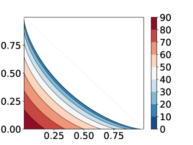
Figure 5: Contours of angle difference between the closest $2$ images over a quadrant of astroid caustic.

4.4 The FSQ and diamond caustic

The two closest images merge when the source crosses the diamond caustic, where $\theta_{23}=0$. Figure 5 shows how $\theta_{23}$ approaches zero as the source approaches the diamond caustic.

The FSQ in Figure 4(a) intersects the $\theta_{23}=0$ plane in an arc that looks very much like the arc in the lower left quadrant of Figure 2

But the midpoint of the FSQ arc is at $(\theta_{12},\theta_{34})=(2\pi/3,2\pi/3)$, putting it 33.3% of the way from the corner at $(\pi,\pi)$ to the corner at $(0,0)$. By comparison, the midpoint of a unit astroid is at $x^{2/3}=y^{2/3}=1/2$, each of which is 35.3% of the semi-axis of the astroid. Hence the shapes are subtly different.

5 Semi-astroidal coordinates

For both the SIEP and the SIQP we have shown that the ACLE has four real solutions if complex quantity, $W$, defined, respectively, in equations (2) and (12) is restricted to lie inside a corresponding unit astroid. For the SIEP the complex quantity is the center of Witt’s hyperbola. For the SIQP, it is the source position scaled by half of the diameter of the diamond caustic. While the diamond caustic reduces to a point under the limiting case of a vanishingly elliptical lens, the potential still forms a stable image configuration if the position of the source relative to the diamond caustic remains the same. This suggests adopting specialized two dimensional coordinate system with one coordinate constant on concentric astroids.

5.1 “Causticity” and position angle

A newly defined quantity should be given both a symbol and a name, with the latter somehow evoking what is being quantified. We name our coordinates making specific reference to the case of a diamond caustic, but note that they apply equally well to describe the position of the Witt-Wynne hyperbola within its unit astroid.

We define a “causticity,” denoted by $\zeta$, that gives the relative displacement of the source towards the astroid. It is the ratio of the size of the concentric astroid on which the source lies to the size of the diamond caustic inside which four images will be produced. If $W$ is given by the position of the source, as in equation (9), then in a coordinate system aligned with the astroid, we define

$$\zeta\equiv\left[\left(\frac{x_{s}}{4\epsilon b}\right)^{2/3}+\left(\frac{y_{s}}{4\epsilon b}\right)^{2/3}\right]^{3/2}.$$ (21)

Loci of constant causticity lie on similar concentric astroids. For the angular position of the source, we use $\phi_{s}$, which represents the angle that the source makes with respect to the symmetry axis. We call these the “semi-astroidal” coordinates.

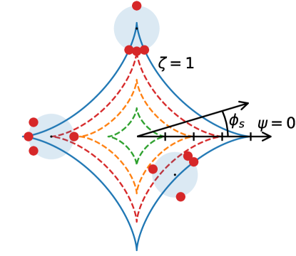
Figure 6: The red dots are quadruple configurations of lensed quasars arising from different source positions within a diamond caustic – the blue astroid for which $\zeta=1$. Two of the pale blue circles are centered at $\zeta=0.95$, with $\phi_{s}=\frac{\pi}{2}$ and $-\frac{\pi}{4}$, respectively. The leftmost configuration has $(\zeta,\phi_{s})=(0.75,\pi)$. The dashed curves are astroids of constant causticity, with $\zeta=0.75$ (red), $\zeta=0.5$ (orange) and $\zeta=0.25$ (green).

Figure 6 shows several configurations corresponding to different semi-astroidal coordinates and how they change as we shift the position of the source within the caustic. Tuan-Anh et al. (2020) also separated the astroid caustic into areas corresponding to different quads according to the Saha & Williams (2003) classification.

Though we have used the source position relative to a diamond caustic to define our coordinates, there are corresponding definitions for the center of the Witt’s hyperbola with respect to the Witt-Wynne diamond.

6 DE-SCRONCHED CONFIGURATIONS OF THE SIS+XS FROM THE ACLE

Until this point, our discussion has focussed on asymptotically circular image configurations. In our treatment of the not-at-all-circular SIQP, we considered only its angular configurations, which give rise to the ACLE despite its non-circularity.

In this section we show that asymptotically circular configurations can be used to produce the quadruple image configurations of a different non-circular potential, the singular isothermal potential with non-vanishing external shear (SIS+XS).

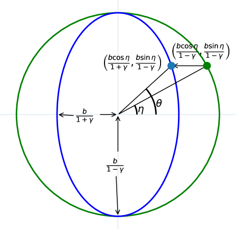
Figure 7: The “scronched” Wynne ellipse for an SIS+XS lens in blue and its auxiliary circle in green. The blue dot is an image formed by the SIS+XS at angle $\theta$; the green dot shows its projection onto the auxiliary circle at $\eta$, the “eccentric angle”.

For the sake of concise description, we make frequent use of the word “scronch,” used by Ellenberg (2021) in his popular book Shape to describe stretching in one direction and squeezing in the orthogonal direction. We show here that a quadruple image configuration for an SIS+XS lens can be “de-scronched” to produce a corresponding asymptotically circular configuration.

The argument proceeds as follows. Luhtaru et al. (2021) have shown that four images for an SIS+XS lens lie at the intersections of a Witt hyperbola and a Wynne ellipse. The positions of those four images, projected onto the auxiliary circle circumscribing the Wynne ellipse have “eccentric angles” $\eta$ that are shown in Section 6.1 to be solutions of the asymptotically circular lens equation.

The diamond caustic for an SIS+XS lens is a “scronched” astroid. For the purpose of tying the positions of sources within these scronched astroids to the positions of sources in the true astroids of their associated asymptotically circular lenses, we define “astroidal coordinates”, causticity and “astroidal angle” for a scronched astroid in Section 6.2. All SIS+XS configurations with the same causticity and astroidal angle de-scronch to the same solution of the ACLE. Given the shear of an SIS+XS lens and the position of the source relative to its scronched astroid, one can solve the lens equation by finding the image configuration for the corresponding asymptotically circular lens and then scronching the configuration.

6.1 De-scronching configurations of the SIS+XS

The potential for the singular isothermal sphere with finite external shear centered on the lens (SIS+XS) is given by,

$$\Phi(x,y)=b\sqrt{x^{2}+y^{2}}-\frac{\gamma}{2}(x^{2}-y^{2})\quad,$$ (22)

with the lensing galaxy at the origin of the coordinate system. This differs from the case considered by Luhtaru et al. (2021) who, following Witt (1996), expand the shear around the source position. In Appendix D we derive expressions for Witt’s hyperbola and Wynne’s ellipse appropriate to our lens-centered coordinate system.

Witt’s hyperbola is given by

$$\frac{(1-\gamma)y-y_{s}}{(1+\gamma)x-x_{s}}=\frac{y}{x}\quad.$$ (23)

Wynne’s ellipse is given by

$$\left[{x-x_{s}/(1+\gamma)\over b/(1+\gamma)}\right]^{2}+\left[{y-y_{s}/(1-\gamma)\over b/(1-\gamma)}\right]^{2}=1\quad.$$ (24)

Note that it is centered neither on the source nor on the lensing galaxy but at

$$(x_{e},y_{e})=\left({x_{s}\over[1+\gamma]},{y_{s}\over[1-\gamma]}\right)\quad.$$ (25)

Taking the shear, $\gamma$ to be positive, Wynne’s ellipse has semi-major axis $b/(1-\gamma)$ along the $y$-direction, perpendicular to the elongation of the potential, semi-minor axis $b/(1+\gamma)$ along the $x$-direction. and axis ratio $(1-\gamma)/(1+\gamma)$.

Figure 7 shows the Wynne ellipse for an SIS+XS configuration along with one of its images. It also shows the auxiliary circle with radius $b/(1-\gamma)$ circumscribing that ellipse. Suppose $(x,y)$ is a solution of the lens for our SIS+XS system, projecting to eccentric angle $\eta$ on the auxiliary circle. Then

$$(x-x_{e},y-y_{e})=\left(\frac{b\cos{\eta}}{1+\gamma},\frac{b\sin{\eta}}{1-\gamma}\right)\quad.$$ (26)

Rewriting this is terms of the source position using Equation (25) and substituting into the numerator and denominator of the left hand side of Witt’s hyperbola, Equation (23), gives

$$(1-\gamma)y-y_{s}=b\sin\eta\quad{\rm and}\quad$$

$$~{}~{}(1+\gamma)x-x_{s}=b\cos{\eta}\quad~{}~{}.~{}\quad$$ (27)

Subtituting into the numerator and denominator of its right hand side gives

$$y=(y_{s}+b\sin\eta)/(1-\gamma)\quad{\rm and}\quad$$

$$x=(x_{s}+b\cos\eta)/(1+\gamma)\quad~{}~{}.~{}~{}\quad$$ (28)

Combining these, the image position on Wynne’s ellipse, $(x,y)$, can be eliminated from the equation for Witt’s hyperbola in favor of its projected eccentric angle $\eta$. It becomes,

$$\frac{\sin{\eta}}{\cos{\eta}}=\left(\frac{1+\gamma}{1-\gamma}\right)\left(\frac{y_{s}+b\sin{\eta}}{x_{s}+b\cos{\eta}}\right).\\$$ (29)

After straightforward algebra detailed in Appendix E, this becomes the asymptotically circular lens equation,

$$e^{4i\eta}-2We^{3i\eta}+2\bar{W}e^{i\eta}-1=0\quad,$$ (30)

with

$$W=\left[\frac{(1-\gamma)x_{s}-i(1+\gamma)y_{s}}{2b\gamma}\right].$$ (31)

The four solutions for $\eta$ give the eccentric angles on the auxiliary ellipse associated with the four lens images on Wynne’s ellipse. The unit astroid bounding $W$ has cusps on the horizontal and vertical axes, respectively, at

$$x_{s}=\pm\left(\frac{2b\gamma}{1-\gamma}\right)~{};~{}y_{s}=\pm\left(\frac{2b\gamma}{1+\gamma}\right)\quad,$$ (32)

which would indicate that the diamond caustic is a scronched astroid elongated in the $x$-direction, perpendicular to Wynne’s ellipse, and given by

$$\left(\frac{(1-\gamma)x}{2\gamma b}\right)^{2/3}+\left(\frac{(1+\gamma)y}{2\gamma b}\right)^{2/3}=1.$$ (33)

We can alternatively define $W$ in terms of the position of the center of Witt’s hyperbola relative to the center of Wynne’s ellipse. Starting with Equation (23) we find

$$(x_{h},y_{h})=\left(\frac{x_{s}}{2\gamma},-\frac{y_{s}}{2\gamma}\right)\quad.$$ (34)

Subtracting Equation (25)

$$x_{h}-x_{e}=~{}~{}\left(\frac{1-\gamma}{1+\gamma}\right)\frac{x_{s}}{2\gamma}\quad\rm{and}\quad$$

$$y_{h}-y_{e}=-\left(\frac{1+\gamma}{1-\gamma}\right)\frac{y_{s}}{2\gamma}~{}~{}\quad~{}.~{}\quad$$ (35)

giving

$$W=\left[\frac{x_{h}-x_{e}}{b/(1+\gamma)}+i\frac{y_{h}-y_{e}}{b/(1-\gamma)}\right].$$ (36)

The unit astroid bounding $W$ has cusps on the horizontal and vertical axes, respectively,

$$x_{h}-x_{e}=\pm\frac{b}{(1+\gamma)}~{};~{}y_{h}-y_{e}=\pm\frac{b}{(1-\gamma)},$$ (37)

which indicates that the Witt-Wynne diamond is a scronched astroid elongated in the $y$-direction,

$$\left(\frac{x}{b/(1+\gamma)}\right)^{2/3}+\left(\frac{y}{b/(1-\gamma)}\right)^{2/3}=1,$$ (38)

which is perpendicular to the diamond caustic, Equation (33) and parallel to Wynne’s ellipse.

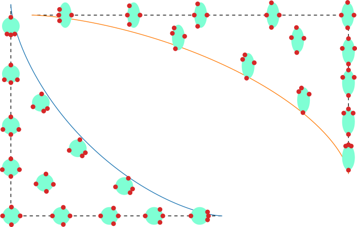
Figure 8: Image configurations for SIS+XS lens systems with the source at various positions in one quadrant of the diamond caustic. The cyan Wynne circles and Wynne ellipses are centered at the source position. The lower left shows the limiting case of shear $\gamma\rightarrow 0$, while the upper right shows $\gamma=1/3$, and has been rotated $180^{\circ}$. The $\gamma\rightarrow 0$ diamond caustic is scronched parallel to the elongation of the potential to produce the $\gamma=1/3$ diamond caustic. The $\gamma=1/3$ Wynne ellipses are scronched perpendicular to the elongation of the potential and the diamond caustic. Apart from the $180^{\circ}$ rotation, the causticities $\zeta$ and astroidal angles $\alpha$ are the same for both sets of configurations.

6.2 Astroidal coordinates

Finch et al. (2002) represent the locus of the SIS+XS diamond caustic parametrically, in terms of $\theta_{c}$, the polar coordinate in the image plane of the point on the critical curve at which two images converge when a source crosses the associated point on the caustic. The locus of the caustic traced by $\theta_{c}$ is given by

$$x_{a}=\frac{2b\gamma}{1-\gamma}\cos^{3}\theta_{c}~{};~{}y_{a}=-\frac{2b\gamma}{1+\gamma}\sin^{3}\theta_{c}\quad.$$ (39)

Note that

$$\tan\phi_{s}=\frac{y_{a}}{x_{a}}=-\frac{1-\gamma}{1+\gamma}\tan^{3}\theta_{c}\quad.\quad$$ (40)

As was evident in Equation (33), the diamond caustic is a scronched astroid, stretched by a factor of $\frac{1}{1-\gamma}$ in the horizontal direction and squeezed by a factor of $\frac{1}{1+\gamma}$ in the vertical direction. As we de-scronch the diamond caustic, maintaining the relative position of the source, $\phi_{s}$, varies as ${(1-\gamma)\over(1+\gamma)}$. Thus $\theta_{c}$ remains unchanged.

The principal result of this section can be succinctly expressed by introducing coordinates that are invariant under scronching. We define an “astroidal angle”, $\alpha$, such that

$$\tan^{3}\alpha\equiv\left(\frac{1+\gamma}{1-\gamma}\right)\tan\phi_{s}\quad.$$ (41)

so that $\alpha=-\eta_{c}$.

We also extend our original definition of causticity, Equation (21) to include non-vanishing shear,

$$\zeta\equiv\left[\left(\frac{(1-\gamma)x_{s}}{2b\gamma}\right)^{2/3}+\left(\frac{(1+\gamma)y_{s}}{2b\gamma}\right)^{2/3}\right]^{3/2},$$ (42)

noting that $\zeta$ is unchanged as one de-scronches the diamond caustic.

We conclude that the image configuration for an SIS+XS lens is a scronched version of the image configuration for the corresponding de-scronched circular lens with the same causticity $\zeta$ and astroidal angle $\alpha$.

6.3 The scronching of the asymptotically circular configurations and their diamond caustic

In Figure 8 we show thirteen quadruple image configurations of the asymptotically circular lens and the corresponding configurations of an SIS+XS lens with identical astroidal coordinates. Each configuration is centered at the position of the source within the diamond caustic. The asymptotically circular astroid is scronched by the same factors as the Wynne circle. but with the axes switched.

7 ACLE SOLUTIONS FOR DE-SCRONCHED CONFIGURATIONS OF THE SIEP

As with the SIS+XS, the image positions for the singular isothermal elliptical potential (SIEP) with non-vanishing ellipticity can also be found by de-scronching Wynne’s ellipse to a circle, solving the asymptotically circular lens equation, and then scronching the configuration.

For the sake of comparision with the SIS+XS, we use semi-ellipticity $\hat{\epsilon}$ (Luhtaru et al., 2021) rather than axis ratio $q$ where

$$\hat{\epsilon}\equiv\frac{1-q}{1+q}\quad.$$ (43)

The SIEP is then

$$\Phi(x,y)=\sqrt{[(1-\hat{\epsilon})x]^{2}+[(1+\hat{\epsilon})y]^{2}}\quad.$$ (44)

The diamond caustic of the SIEP is not a scronched astroid, but the positions of its four images can nonetheless be found at the intersection of a Wynne ellipse and a Witt hyperbola (Luhtaru et al., 2021). We show here that the Witt-Wynne diamond is a scronched astroid, as was the case for the SIS+XS.

Wynne’s ellipse is elongated perpendicular to the long axis of the potential and is given by

$$\left[{x-x_{s}\over b/(1+\hat{\epsilon})}\right]^{2}+\left[{y-y_{s}\over b/(1-\hat{\epsilon})}\right]^{2}=1\quad.$$ (45)

This differs trivially from Wynne’s ellipse the SIS+XS, Equation (24) in the replacement of the shear, $\gamma$ with the semi-ellipticity, $\hat{\epsilon}$, but non-trivially in that, in contrast to the SIS+XS, the ellipse for the SIEP is centered on the source position.

Witt’s hyperbola is given by

$$[(y-y_{s})-(y_{h}-y_{s})] [(x-x_{s})(x_{h}-x_{s})]$$ (46)

$$=a^{2}/2\quad,$$

where $a$ is the semi-major axis of the hyperbola. It can be evaluated by substituting the center of Wynne’s ellipse, $(x_{s},y_{s})$, which must, by construction, lie on Witt’s hyperbola, for $x$ and $y$ in Equation (46), giving

$$a^{2}/2=(y_{h}-y_{s})(x_{h}-x_{s})\quad.$$ (47)

Witt’s hyperbola then simplifies to

$$(y-y_{s})(x-x_{s})-(y-y_{s})(x_{h}-x_{s})\quad\quad\quad$$

$$-(x-x_{s})(y_{h}-y_{s})=0.\quad$$ (48)

Though it was introduced for the SIS+XS, Figure 7 can equally well be applied to the SIEP. If $(x,y)$ is a solution of the lens equation for a SIEP system, projecting to eccentric angle $\eta$ on the auxiliary circle gives

$$(x-x_{s},y-y_{s})=\left(\frac{b\cos{\eta}}{1+\hat{\epsilon}},\frac{b\sin{\eta}}{1-\hat{\epsilon}}\right)\quad.$$ (49)

Substituting this general point on the Wynne’s ellipse into the equation for Witt’s hyperbola, we get

$$\sin\eta\cos\eta = -(1+\hat{\epsilon})\sin\eta(x_{h}-x_{s})/b$$ (50)

$$-(1-\hat{\epsilon})\cos\eta(y_{h}-y_{s})/b~{}.$$

Dividing by $\sin\eta\cos\eta$ and letting

$$p = (1+\hat{\epsilon})(x_{h}-x_{s})/b~{}~{}~{}{\rm and}$$ (51)

$$q = (1-\hat{\epsilon})(y_{h}-y_{s})/b~{}~{}~{}~{}~{}.$$ (52)

we have

$$1=p\sec\eta+q\csc\eta\quad,$$ (53)

which is exactly the deceptively simple form of the ACLE, Equation (8). In the defining form of the ACLE, Equation (1), the quantity W becomes

$$W=\left[\frac{x_{h}-x_{s}}{b/(1+\hat{\epsilon})}+i\frac{y_{h}-y_{s}}{b/(1-\hat{\epsilon})}\right].$$ (54)

The corresponding value for the SIS+XS, Equation (36) differs only in that it explicitly depends on the center of Wynne’s ellipse, $(x_{e},y_{e})$ rather than implicitly through the source position.

As with the SIS+XS, the Witt-Wynne diamond is a scronched astroid elongated parallel to the Wynne ellipse and perpendicular to the potential. Unlike the case for the SIS+XS, the diamond caustic is not a scronched astroid.

8 Generalization to all circularly symmetric potentials

Until now we have analyzed the properties of circular configurations as limiting cases of specific potentials. However, these properties also hold more generally for all circularly symmetric potentials. Specifically, An (2005) showed that the caustic locus depends only on “the azimuthal behavior of perturbation of the potential.” He then showed that potentials with ellipticity, external shear, and quadrupole moment can all be shown to have perturbations of identical form to first order in the limit of vanishing quadrupole.

This implies that the angular configurations (and the ratio of magnifications) are identical for potentials with any of the three abovementioned deviations from circularity, up to linear order in the perturbations.

In this section we show that a generic circular potential with vanishing external shear gives rise to a Witt hyperbola, with images forming where that hyperbola crosses a 1D locus, the limiting Wynne circle.

Our generic circular potential with shear can be written

$$\Phi(x,y)=f(x^{2}+y^{2})-\frac{\gamma}{2}(x^{2}-y^{2}).$$ (55)

Using the lens equation(Bourassa & Kantowski, 1975),

$$\mathbf{r}-\mathbf{r}_{s}=\nabla{\Phi(\mathbf{r})},$$ (56)

we get

$$x-x_{s} = 2xf^{\prime}(x^{2}+y^{2})-\gamma x\quad{\rm and}$$ (57)

$$y-y_{s} = 2yf^{\prime}(x^{2}+y^{2})+\gamma y\quad.$$ (58)

Rearranging and dividing Equation (58) by Equation (57), we obtain the equation of Witt’s hyperbola, on which all four images should lie,

$$\frac{(1-\gamma)y-y_{s}}{(1+\gamma)x-x_{s}}=\frac{y}{x}.$$ (59)

This is exactly Witt’s hyperbola for an SIS+XS potential. By rearranging and squaring Equations (57) and (58), we can obtain a one dimensional locus that reduces to Wynne’s ellipse for the case of SIS+XS,

$$((1+\gamma)x-x_{s})^{2}+((1-\gamma)y-y_{s})^{2}$$

$$=4\gamma^{2}(x^{2}+y^{2})(f^{\prime}(x^{2}+y^{2}))^{2}$$ (60)

In the limiting case of vanishing shear, ($\gamma\rightarrow 0,x_{s}\rightarrow 0,y_{s}\rightarrow 0$), and after taking the square root, Equation (60) becomes

$$f^{\prime}(x^{2}+y^{2})=1/2\quad.$$ (61)

Thus images form on a circle with squared radius $a^{2}=x^{2}+y^{2}$.

Figure 9: Outer circle: images for two different source positions for 1 point mass lens with asymptotically vanishing shear and lens strength $b=1.25$. Inner circle: images formed by an SIS lens with vanishing shear ($\gamma\rightarrow 0$) and $b=1$, The source positions have the same causticity and astroidal angle for both circles, but the symmetry axes of the two configurations have been rotated to avoid confusion. Keeton’s lensmodel (Keeton, 2010) has been used to verify the configurations.

As the configurations for an asymptotically circular lens are given by the intersection of a circle and a hyperbola, the positions are exactly the same as those we previously encountered for isothermal potentials in the limiting circular case.

Figure 9 shows the predicted positions for a point mass lens and the SIS+XS potential in the limiting case.

9 Flux ratios for the images in asymptotically circular configurations

As the area of the caustic decreases, the inverse magnification tends to $0$, and hence, the brightnesses of all 4 images grow infinite. It is nonetheless possible to calculate the ratios of the brightnesses of the 4 images in the limiting case of circularity.

In Appendix F we derive the expressions for magnifications of images formed by the SIQP and the SIS+XS potential with non-vanishing quadrupole. In asymptotically circular cases, with either $\gamma\rightarrow 0$ or $\epsilon\to 0$ and $s\rightarrow 0$, the magnification simplifies to

$$\mu_{SIQP} = \frac{b}{s\cos(\theta-\phi_{s})-4\epsilon b\cos(2\theta)}~{}{\rm and}\quad\quad$$ (62)

$$\mu_{SIS+XS} = \frac{b}{s\cos(\theta-\phi_{s})-2\gamma b\cos(2\theta)}\quad,$$ (63)

where $(s,\phi_{s})$ are the polar coordinates of source, and $\theta$ is the polar angle of an image on the limiting circle.

We also show in Appendix F that if an SIQP lens system and an SIS+XS lens system produce the same asymptotically circular configuration, the quadrupole parameter $\epsilon$, of the SIQP is equal to the shear parameter, $\gamma$ of the SIS+XS. The magnifications for the SIS+XS system, Equation (63), are then twice the magnifications for the corresponding SIQP system, Equation (62). The SIS+XS has a diamond caustic that is half the area of the diamond caustic for the SIQP (both of which are true astroids in the limit of circularity).

An (2005) showed that for small perturbations, the magnification ratios depend only on the angular behavior of the potential, but that the magnifications are scaled by a different multiplicative factors for different spherically symmetric mass distributions.

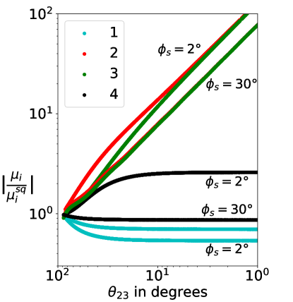
Figure 10: Image magnifications for asymptotically circular image configurations, relative to the image magnifications for a source at the center of the diamond caustic. Two cases are shown, one with the source close to an axis of the diamond caustic $(\phi_{s}=2^{\circ})$, and a second far from either axis $(\phi_{s}=30^{\circ})$. The two closest images (those on the secondary branch of Witt’s hyperbola) increase in brightness inversely as their separation. By contrast, the relative magnifications of the images at $\theta_{1}$ and $\theta_{4}$ on the primary branch of Witt’s hyperbola vary only by factors of order unity and quickly reach limiting values, even in the cusp-like case of $\phi_{s}=2^{\circ}$. The convention is that of Section 4.1.

Figure 10 shows how magnification varies for images formed by an asymptotically circular potential as $\theta_{23}$ (the angle between the closest images) varies. The magnifications of images $2$ and $3$ asymptote to a straight lines of unit slope in the inverted log-log graph. This follows from the theorem that the magnification is approximately inversely proportional to the angular separation between the images (Schneider et al., 1992, p. 190).

10 Solar System Occultation Flashes and the ACLE

The wide applicability of asymptotically circular image configurations extends even beyond gravitational lensing.

Nicholson et al. (1995) noted the parallel between gravitational lensing and the “central flash” observed in their observations of Saturn’s occultation of 28 Sgr on 3 July 1989. The star never completely disappears behind the planet. A refracted image on Saturn’s limb grows increasingly faint following ingress. At the same time a second, even fainter, refracted image brightens on the opposite limb. Toward mid-occultation a bright new pair of images forms causing the first of two flashes. The images grow fainter as they move apart, but one of them grows brighter again just before it merges with the original image, which also grows brighter.

Their observations were sufficiently sensitive to show the two bright images of the newly created pair but not the fainter images, whose positions they calculate based on an assumed atmosphere.

Their Figure 4 shows theoretical calculations of a series of configurations over the course of their observations. We measured the positions of the images directly from the figure and then de-scronched them (taking Saturn’s limb to be elliptical) to an auxiliary circle, as in Section 6.

The two larger eccentric angle differences, $\eta_{12}$ and $\eta_{34}$ were used to “predict” the smallest eccentric angle difference, $\eta_{23}$ using Equation 20. The deviations of the measured $\eta_{23}$ from the calculated $\eta_{23}$ have a mean of $-0.455^{\circ}$ with a standard deviation of $1.04^{\circ}$.

By comparison, Woldesenbet & Williams (2012) found that only 12 out of 40 observed quads lie within $2^{\circ}$ of the Fundamental Surface of Quads. This raises the possibility that the image configurations associated with occultation flashes may be more like those expected for quadruply lensed quasars than the quasar configurations themselves.

11 Discussion and Conclusions

We have examined the circular image configurations of quadruply lensed sources. These occupy a two-dimensional space bounded by a suitably defined unit astroid. We define astroidal coordinates, “causticity”, $\zeta$, and “astroidal angle”, $\alpha$, on this space.

We considered a variety of distinct cases that give rise to such configurations, first nearly-circular isothermal potentials with vanishing ellipticity or shear and then nearly-circular non-isothermal potentials with vanishing shear. Across these different cases, systems with identical astroidal coordinates produce identical angular configurations.

We discussed the non-circular singular isothermal quadrupole lens, and showed that it produces the same set of angular configurations (with angles measured from the position of the lensing galaxy) even though the images do not lie on a circle.

We extended our analysis to singular isothermal potentials of non-vanishing ellipticity and circular isothermal potentials with non-vanishing shear and showed that their image configurations are “scronched” versions of the asymptotically circular configurations – stretched in one direction and squeezed in the other, as in Figure 8. We extended our definitions of astroidal coordinates to incorporate these, and found that systems with identical $\zeta$ and $\alpha$ have identical angular configurations when “de-scronched”.

The Witt-Wynne geometric solution for the SIEP helps to explain the frequent resurfacing of these configurations. Witt found that for non-vanishing elliptical potentials and for singular isothermal potentials with external shear, the four images must lie on a hyperbola. Wynne found that the images for both cases must lie on an ellipse if the potentials are isothermal.

Images formed at the intersection of a Witt hyperbola and a Wynne ellipse of vanishing ellipticity (a circle) give an asymptotically circular image configuration. “Scronching” that circle to an ellipse gives a configuration for a lens with non-vanishing quadrupole.

Appendix A The ACLE as an edge case of the Witt-Wynne construction

We derive the asymptotically circular lens equation (ACLE) from the limiting case of the Witt-Wynne construction. In this geometric scheme, the four image positions lie at the intersections of a circle and a hyperbola. To simplify the situation, we can translate and rescale our coordinate system, such that the Wynne ellipse is a circle of radius $b$ centered at the origin and the hyperbola passes through the origin, as it should pass through the center of the circle.

Let the images be at polar angles $\theta_{1},\theta_{2},\theta_{3},$ and $\theta_{4}$. For simplicity, rotate the configuration such that the major axis of the potential is at $\psi=0$. The general equation of a rectangular hyperbola passing through the origin whose asymptotes are aligned with the coordinate axes is

$$(x-x_{h})(y-y_{h})=x_{h}y_{h}$$ (A1)

Substituting a general point from the circle, ${(b\cos\theta,b\sin\theta)}$, we find

$$b^{2}\sin\theta\cos\theta-bx_{h}\sin\theta-by_{h}\cos\theta=0\quad$$ (A2)

and hence

$$1=\frac{x_{h}}{b}\sec\theta+\frac{y_{h}}{b}\csc\theta\quad.$$ (A3)

This is the more compact of our two versions of the ACLE.

Defining $p\equiv\frac{x_{h}}{b}$ and $q\equiv\frac{y_{h}}{b}$, one can show that $|p\sec\theta+q\csc\theta|$ attains a local minimum with value $(p^{2/3}+q^{2/3})^{3/2}$. Equation (A3) will therefore have $4$ distinct solutions when

$$(p^{2/3}+q^{2/3})^{3/2}<1\quad{\rm or}$$

$$p^{2/3}+q^{2/3}<1~{}~{}~{},~{}$$ (A4)

and $2$ real solutions when the inequality is reversed. Two of the solutions merge to a single solutions when equality holds. Curves of constant $p^{2/3}+q^{2/3}$ trace similar astroids in the $(p,q)$ plane.

From equation (A2) we obtain

$$b^{2}\sin 2\theta-2bx_{h}\sin\theta-2by_{h}\cos\theta=0,$$ (A5)

The four polar angles of the lens configuration, $\theta_{1},\theta_{2},\theta_{3},$ and $\theta_{4}$ are the solutions of this equation. Replacing $\cos\alpha$ with $\frac{e^{i\alpha}+e^{-i\alpha}}{2}$ and $\sin\alpha$ with $\frac{e^{i\alpha}-e^{-i\alpha}}{2i}$, we obtain the equation:

$$b^{2}\left(\frac{e^{2i\theta}-e^{-2i\theta}}{2i}\right)-2bx_{h}\left(\frac{e^{i\theta}-e^{-i\theta}}{2i}\right)-2by_{h}\left(\frac{e^{i\theta}+e^{-i\theta}}{2}\right)=0$$

$$e^{4i\theta}-2\left(\frac{x_{h}+iy_{h}}{b}\right)e^{3i\theta}+2\left(\frac{x_{h}-iy_{h}}{b}\right)e^{i\theta}-1=0$$ (A6)

Note that if we let

$$W=\frac{x_{h}+iy_{h}}{b},$$ (A7)

Equation (A6) becomes

$$e^{4i(\theta-\psi)}-2We^{3i(\theta-\psi)}+2\overline{W}e^{i(\theta-\psi)}-1=0,$$ (A8)

where $\theta$ is replaced with $\theta-\psi$ for cases when $\psi\neq 0$. This our second, more useful version of the ACLE.

Taking $\psi=0$ for the sake of clarity, we can apply Vieta’s formula to the coefficient of $e^{3i\theta}$ term,

$$\sum_{j=1}^{4}e^{i\theta_{j}}=2W=2\left(\frac{x_{h}+iy_{h}}{b}\right).$$ (A9)

So, the center of Witt’s hyperbola can be expressed as

$$x_{h}=\frac{b}{2}\sum_{j=1}^{4}\cos\theta_{j}=2\sum_{j=1}^{4}\frac{x_{j}}{4}=2{x_{\textrm{\scriptsize centroid}}}$$

$$y_{h}=\frac{b}{2}\sum_{j=1}^{4}\sin\theta_{j}=2\sum_{j=1}^{4}\frac{y_{j}}{4}=2{y_{\textrm{\scriptsize centroid}}}$$ (A10)

Appendix B Closed form solution of the ACLE

The Asymptotically Circular Lens Equation (1),

$$e^{4i\theta}-2We^{3i\theta}+2\overline{W}e^{i\theta}-1=0\quad,$$ (B1)

is quartic in the quantity $z=e^{i\theta}$.

Ferrari’s oft-deprecated method can be used to find four closed form solutions. One juggles the terms in the equation (adding quantities to both sides as needed), so that one has perfect squares on both sides: a quadratic expression in $z$ squared on one side and expression linear in $z$, also squared, on the other. One takes the square root and adds (and subtracts) the quadratic and linear expressions, giving two new quadratics in $z$, which one then solves giving four roots.

There is art in the juggling, creating the two perfect squares. Almost without exception, it is never possible using only the terms in the original quartic. But if one judiciously adds terms that include an unknown algebraic quantity to both sides, one can solve for values of that quantity that give two perfect squares.

We begin by isolating the $z^{4}$ and $z^{3}$ terms on one side of the equation,

$$z^{4}-2Wz^{3}=-2\overline{W}z+1\quad.$$ (B2)

Adding $W^{2}z^{2}$ to both sides gives us

$$z^{4}-2Wz^{3}+W^{2}z^{2}=(z^{2}-Wz)^{2}=W^{2}z^{2}-2\overline{W}z+1\quad.$$ (B3)

The left hand side is a perfect square of a quadratic, but the right hand side is not a perfect square of a linear function. We add terms involving the algebraic quantity $u$, to both sides,

$$\left(z^{2}-Wz+\frac{u}{2}\right)^{2}=(W^{2}+u)z^{2}-(2\overline{W}+Wu)z+\left(1+\frac{u^{2}}{4}\right)\quad.$$ (B4)

The left hand side is again a perfect square, for all values of $u$. The right hand side might be a perfect square for some specific values of $u$.

If such values exist, there is a constant $k$ such that

$$(z\sqrt{W^{2}+u}-k)^{2}=(W^{2}+u)z^{2}-(2\overline{W}+Wu)z+\left(1+\frac{u^{2}}{4}\right)\quad.$$ (B5)

The coefficients of the $z^{1}$ and $z^{0}$ terms give two distinct expressions for $k$. As they must be equal, we have

$$k=\frac{2\overline{W}+Wu}{2\sqrt{W^{2}+u}}={{\sqrt{1+u^{2}/4}}}\quad,$$ (B6)

which gives a cubic equation in $u$,

$$u^{3}+4(1-W\overline{W})u+4(W^{2}-\overline{W}^{2})=0\quad.$$ (B7)

The solution to the cubic can be found from Cardano’s formula, with a root

$$u_{1}=\left(\sqrt[3]{2(\overline{W}^{2}-W^{2})+8\sqrt{A}}+\sqrt[3]{2(\overline{W}^{2}-W^{2})-8\sqrt{A}}\right)\quad$$ (B8)

where

$$A\equiv\frac{1}{27}(1-W\overline{W})^{3}+\frac{W^{2}-\overline{W}^{2}}{16}\quad.$$ (B9)

Using equations (B5) and (B6) our original quartic can be re-written as

$$\left(z^{2}-Wz+\frac{u}{2}\right)^{2}=(W^{2}+u)\left(z-\frac{\sqrt{u^{2}/4+1}}{\sqrt{W^{2}+u}}\right)^{2}$$ (B10)

Taking square roots of both sides, we get a quadratic equation for z

$$\left(z^{2}-Wz+\frac{u}{2}\right)=\widehat{\pm}\left(z\sqrt{W^{2}+u}-\sqrt{u^{2}/4+1}\right)$$ (B11)

with solution

$$2e^{i\theta} = W\widehat{\pm}\sqrt{u+W^{2}}$$ (B12)

$$\widetilde{\pm} \sqrt{(W\widehat{\pm}\sqrt{u+W^{2}})^{2}-2\left(u\widehat{\pm}\sqrt{u^{2}+4}\right)}\quad,$$

Note that $\widehat{\pm}$ arises from taking the square root of the quartic while $\widetilde{\pm}$ arises from the solution of the resulting quadratic. We then have four solutions, $\theta_{\widehat{+}\widetilde{+}}$, $\theta_{\widehat{+}\widetilde{-}}$, $\theta_{\widehat{-}\widetilde{+}}$ and $\theta_{\widehat{-}\widetilde{-}}$.

Appendix C Derivation of the Kassiola & Kovner configuration Invariant

Let $\theta_{1},\theta_{2},\theta_{3},\theta_{4}$ be the 4 different solutions of the ACLE measured with respect to the position angle of the major axis of the potential, $\psi$, which we may take to be zero without loss of generality,

$$Ae^{4i\theta}+Be^{3i\theta}+Ce^{2i\theta}+De^{i\theta}+E=0,$$ (C1)

where $C=0$. Applying Vieta’s formula to the coefficient of $2^{nd}$ degree in equation (C1), we have

$$C=e^{i(\theta_{1}+\theta_{2})}+e^{i(\theta_{3}+\theta_{4})}+e^{i(\theta_{1}+\theta_{3})}+e^{i(\theta_{2}+\theta_{4})}+e^{i(\theta_{1}+\theta_{4})}+e^{i(\theta_{2}+\theta_{3})}=0.$$ (C2)

Using the property,

$$e^{i\alpha}+e^{i\beta}=2\cos\left(\frac{\alpha-\beta}{2}\right)e^{i\frac{\alpha+\beta}{2}},$$

we observe that

$$\mkern-36.0mu2\cos\frac{\theta_{1}+\theta_{2}-\theta_{3}-\theta_{4}}{2}e^{i\frac{\theta_{1}+\theta_{2}+\theta_{3}+\theta_{4}}{2}}+2\cos\frac{\theta_{1}+\theta_{3}-\theta_{2}-\theta_{4}}{2}e^{i\frac{\theta_{1}+\theta_{2}+\theta_{3}+\theta_{4}}{2}}\quad\quad$$

$$+2\cos\frac{\theta_{1}+\theta_{4}-\theta_{2}-\theta_{3}}{2}e^{i\frac{\theta_{1}+\theta_{2}+\theta_{3}+\theta_{4}}{2}}=0,$$ (C3)

implying

$$\cos\frac{\theta_{1}+\theta_{2}-\theta_{3}-\theta_{4}}{2}+\cos\frac{\theta_{1}+\theta_{3}-\theta_{2}-\theta_{4}}{2}+\cos\frac{\theta_{1}+\theta_{4}-\theta_{2}-\theta_{3}}{2}=0,$$ (C4)

which is the Kassiola & Kovner (1995) configuration invariant.

One can restore full generality using a second relation derived by Kassiola and Kovner, giving the major axis of the potential,

$$\psi=\frac{\theta_{1}+\theta_{2}+\theta_{3}+\theta_{4}}{4}\pm\frac{\pi}{4}\quad.$$ (C5)

With similar algebraic gymnastics one can derive the ACLE from the configuration invariant.

Appendix D The Witt-Wynne construction for lens-centered shear

Luhtaru et al. (2021) expanded the Witt-Wynne construction of Wynne & Schechter (2018) to the more general case of an SIEP potential with external shear (XS) aligned with the ellipticity. Following Witt (1996)’s initial development they took the shear to be centered on the source. We show here that the Witt-Wynne construction also works for a singular isothermal sphere (SIS) with lens-centered shear,

$$\Phi(x,y)=b\sqrt{x^{2}+y^{2}}-\frac{\gamma}{2}(x^{2}-y^{2})\quad,$$ (D1)

giving a potential elongated along the x-axis for positve shear.

Starting with the lens equation,

$$\mathbf{r}-\mathbf{r}_{s}=\nabla{\Phi(\mathbf{r})},$$ (D2)

we get

$$x-x_{s} = \frac{bx}{\sqrt{x^{2}+y^{2}}}-\gamma x\quad{\rm and}$$ (D3)

$$y-y_{s} = \frac{by}{\sqrt{x^{2}+y^{2}}}+\gamma y\quad,$$ (D4)

which can be rewritten as

$$(1+\gamma)x-x_{s} = \frac{bx}{\sqrt{x^{2}+y^{2}}}\quad{\rm and}$$ (D5)

$$(1-\gamma)y-y_{s} = \frac{by}{\sqrt{x^{2}+y^{2}}}\quad.$$ (D6)

Dividing Equation (D6) by Equation (D5), we get the equation for Witt’s hyperbola on which all four images should lie,

$$\frac{(1-\gamma)y-y_{s}}{(1+\gamma)x-x_{s}}=\frac{y}{x}\quad,$$ (D7)

which is centered at

$$(x_{h},y_{h})=\left(\frac{x_{s}}{2\gamma},-\frac{y_{s}}{2\gamma}\right)\quad.$$ (D8)

Squaring Equations (D5) and (D6) and adding gives us the Wynne ellipse,

$$\left[{x-x_{s}/(1+\gamma)\over 1/(1+\gamma)}\right]^{2}+\left[{y-y_{s}/(1-\gamma)\over 1/(1-\gamma)}\right]^{2}=b^{2}\quad.$$ (D9)

It is stretched along the $y$-axis (the short axis of the potential in our convention) by $1/(1-\gamma)$ and squeezed along the $x$-axis by $1/(1+\gamma)$. The axis ratio of Wynne’s ellipse is therefore

$$q=\left(\frac{1-\gamma}{1+\gamma}\right)\quad.$$ (D10)

Note that in contrast to the source-centered shear case, the center of Wynne’s ellipse is not coincident with the source but is given instead by

$$(x_{e},y_{e})=\left(\frac{x_{s}}{1+\gamma},\frac{y_{s}}{1-\gamma}\right)\quad.$$ (D11)

The center of the ellipse lies on the hyperbola, as expected for the Witt-Wynne construction.

Appendix E The ACLE in terms of eccentric angle $\eta$: algebraic details

Equation (29) in Section 6.1 gives Witt’s hyperbola recast in terms of the eccentric angle $\eta$ on the auxiliary circle that corresponds to a solution of the lens equation on Wynne’s ellipse,

$$\frac{\sin{\eta}}{\cos{\eta}}=\left(\frac{1+\gamma}{1-\gamma}\right)\left(\frac{y_{s}+b\sin{\eta}}{x_{s}+b\cos{\eta}}\right)\quad,\\$$ (E1)

where the coordinates of the source are relative to the center of the lens. Substituting $\sin{\alpha}=\frac{e^{i\alpha}-e^{-i\alpha}}{2i}$ and $\cos{\alpha}=\frac{e^{i\alpha}+e^{-i\alpha}}{2}$ in Equation (E1) gives

$$\frac{1}{i}\frac{e^{i\eta}-e^{-i\eta}}{e^{i\eta}+e^{-i\eta}}=\left(\frac{1+\gamma}{1-\gamma}\right)\frac{2y_{s}+b\left(\frac{e^{i\eta}-e^{-i\eta}}{i}\right)}{2x_{s}+b(e^{i\eta}+e^{-i\eta})}\quad.$$ (E2)

Cross multiplying we have

$$2x_{s}(1-\gamma)(e^{3i\eta}-e^{i\eta})+b(1-\gamma)(e^{4i\eta}-1)=2iy_{s}(1+\gamma)(e^{3i\eta}+e^{i\eta})+b(1+\gamma)(e^{4i\eta}-1)$$

$$(e^{4i\eta}-1)\left(2b\gamma\right)-2e^{3i\eta}((1-\gamma)x_{s}-i(1+\gamma)y_{s})+2e^{i\eta}((1-\gamma)x_{s}+i(1+\gamma)y_{s})=0\quad,$$ (E3)

which after gathering terms gives

$$e^{4i\eta}-2\left(\frac{(1-\gamma)x_{s}-i(1+\gamma)y_{s}}{2b\gamma}\right)e^{3i\eta}+2\left(\frac{(1-\gamma)x_{s}+i(1+\gamma)y_{s}}{2b\gamma}\right)e^{i\eta}-1=0\quad.$$ (E4)

If we let

$$W=\frac{(1-\gamma)x_{s}-i(1+\gamma)y_{s}}{2b\gamma}$$ (E5)

we have

$$e^{4i\eta}-2We^{3i\eta}+2\bar{W}e^{i\eta}-1=0\quad,$$ (E6)

which is precisely the asymptotically circular lens equation. The eccentric angles associated with elliptical configurations formed by SIS+XS are therefore solutions of the ACLE.

Appendix F Image Magnifications for the SIQP and the SIS+XS potential

F.1 The singular isothermal quadrupole

The expression of inverse magnification for each image is given by the determinant of the Jacobian, which Finch et al. (2002) give as

$$\mu^{-1}_{i}=\left(1-\frac{\partial^{2}{\Phi}}{\partial x^{2}}\right)\left(1-\frac{\partial^{2}{\Phi}}{\partial y^{2}}\right)-\left(\frac{\partial^{2}{\Phi}}{\partial{x}\partial y}\right)^{2}$$ (F1)

Calculating and substituting the respective partial derivatives, we get

$$\mu_{SIQP}^{-1}=1-\frac{b(1+3\epsilon\cos(2\theta))}{r},$$ (F2)

where $(r,\theta)$ are the polar coordinates of the image with $x$-axis as the symmetry axis.

We can eliminate $r$ by insisting that the image must form at a stationary point of the time delay,

$$t(\vec{r})=\frac{D}{c}\left(\frac{1}{2}(\vec{r}-\vec{s})^{2}-\Phi(\vec{r})\right)\quad,$$ (F3)

which can be rewritten, upto additive and multiplicative constants, as

$$\tilde{t}(r,\theta)=\frac{1}{2}r^{2}-rs\cos(\theta-\phi_{s})-\Phi(r,\theta)\quad.$$ (F4)

The stationarity condition for the time delay at the images is $\frac{\partial\tilde{t}}{\partial r}=0$ and $\frac{1}{r}\frac{\partial\tilde{t}}{\partial\theta}=0$, the former of which gives

$$r=s\cos(\theta-\phi_{s})+b(1-\epsilon\cos 2\theta)$$ (F5)

for each of the four images. Substituting $r$ from Equation (F5) into Equation (F2), we get

$$\mu_{SIQP}^{-1}=\frac{s\cos(\theta-\phi_{s})-4\epsilon b\cos(2\theta)}{s\cos(\theta-\phi_{s})+b(1-\epsilon\cos(2\theta))}.$$ (F6)

F.2 The Singular Isothermal Sphere with External Shear

The magnifications of the images produced from SIS+XS potential are similarly found to be

$$\mu^{-1}_{SIS+XS}=\left(1-\frac{\tilde{b}y^{2}}{(x^{2}+y^{2})^{3/2}}+\gamma\right)\left(1-\frac{\tilde{b}x^{2}}{(x^{2}+y^{2})^{3/2}}-\gamma\right)-\left(-\frac{\tilde{b}xy}{(x^{2}+y^{2})^{3/2}}\right)^{2}$$

$$=1-\gamma^{2}-\frac{\tilde{b}}{\sqrt{x^{2}+y^{2}}}-\frac{\tilde{b}\gamma(x^{2}-y^{2})}{(x^{2}+y^{2})^{3/2}}\quad.$$

$$=1-\gamma^{2}-\frac{\tilde{b}}{r}\left[{1+\gamma\cos(2\tilde{\theta})}\right]$$ (F7)

Note that we use $\tilde{\theta}$ and $\theta$ to distinguish between the polar angles of images formed by the SIS+XS and SIQP, respectively.

From the stationarity requirement, we have

$$r-\tilde{s}\cos(\tilde{\theta}-\tilde{\phi}_{s})-\tilde{b}+\gamma r\cos 2\tilde{\theta}=0$$ (F8)

and

$$\frac{1}{r}=\frac{1+\gamma\cos 2\tilde{\theta}}{\tilde{b}+\tilde{s}\cos(\tilde{\theta}-\tilde{\phi}_{s})}$$ (F9)

Substituting $\frac{1}{r}$ into Equation (F.2),

$$\mu^{-1}_{SIS+XS}=1-\gamma^{2}-\tilde{b}\left({\frac{1+\gamma\cos 2\tilde{\theta}}{\tilde{b}+\tilde{s}\cos(\tilde{\theta}-\tilde{\phi}_{s})}}\right)\left[1+\gamma\cos(2\tilde{\theta})\right]$$

$$\mu_{SIS+XS}=\frac{\tilde{b}+\tilde{s}\cos(\tilde{\theta}-\tilde{\phi}_{s})}{(1-\gamma^{2})\tilde{s}\cos(\tilde{\theta}-\tilde{\phi}_{s})-2\tilde{b}\gamma\cos{2\tilde{\theta}}-\tilde{b}\gamma^{2}(1+\cos^{2}{2\tilde{\theta}})}$$ (F10)

References

- An (2005) An, J. H. 2005, Monthly Notices of the Royal Astronomical Society, 356, 1409, doi: 10.1111/j.1365-2966.2004.08581.x
- Bourassa & Kantowski (1975) Bourassa, R. R., & Kantowski, R. 1975, ApJ, 195, 13, doi: 10.1086/153300
- Chang & Refsdal (1979) Chang, K., & Refsdal, S. 1979, Nature, 282, 561, doi: 10.1038/282561a0
- Dalal (1998) Dalal, N. 1998, The Astrophysical Journal, 509, L13, doi: 10.1086/311761
- Ellenberg (2021) Ellenberg, J. 2021, Shape: The Hidden Geometry of Information, Biology, Strategy, Democracy, and Everything Else (Penguin Publishing Group). https://books.google.com/books?id=ZC4MEAAAQBAJ
- Finch et al. (2002) Finch, T. K., Carlivati, L. P., Winn, J. N., & Schechter, P. L. 2002, The Astrophysical Journal, 577, 51, doi: 10.1086/342163
- Kassiola & Kovner (1995) Kassiola, A., & Kovner, I. 1995, Monthly Notices of the Royal Astronomical Society, 272, 363, doi: 10.1093/mnras/272.2.363
- Keeton (2010) Keeton, C. R. 2010, General Relativity and Gravitation, 42, 2151, doi: 10.1007/s10714-010-1041-1
- Kochanek (1991) Kochanek, C. S. 1991, ApJ, 373, 354, doi: 10.1086/170057
- Kormann et al. (1994) Kormann, R., Schneider, P., & Bartelmann, M. 1994, A&A, 284, 285
- Luhtaru et al. (2021) Luhtaru, R., Schechter, P. L., & de Soto, K. M. 2021, The Astrophysical Journal, 915, 4, doi: 10.3847/1538-4357/abfda1
- Nicholson et al. (1995) Nicholson, P. D., McGhee, C. A., & French, R. G. 1995, Icarus, 113, 57, doi: 10.1006/icar.1995.1005
- Ohanian (1983) Ohanian, H. C. 1983, ApJ, 271, 551, doi: 10.1086/161221
- Saha & Williams (2003) Saha, P., & Williams, L. L. R. 2003, The Astronomical Journal, 125, 2769, doi: 10.1086/375204
- Schechter & Wynne (2019) Schechter, P. L., & Wynne, R. A. 2019, The Astrophysical Journal, 876, 9, doi: 10.3847/1538-4357/ab1258
- Schneider et al. (1992) Schneider, P., Ehlers, J., Ehlers, J., & Falco, E. 1992, Gravitational Lenses, Astronomy and astrophysics library (Springer-Verlag). https://books.google.com/books?id=3V-3QgAACAAJ
- Tuan-Anh et al. (2020) Tuan-Anh, P., Thai, T. T., Tuan, N. A., et al. 2020, Journal of The Korean Astronomical Society, 53, 149. https://arxiv.org/abs/2011.13142
- Witt (1996) Witt, H. J. 1996, The Astrophysical Journal, 472, L1, doi: 10.1086/310358