Real-time Monitoring of Functional Data

Abstract

With the rise of Industry 4.0, huge amounts of data are now generated that are apt to be modelled as functional data. In this setting, standard profile monitoring methods aim to assess the stability over time of a completely observed functional quality characteristic. However, in some practical situations, evaluating the process state in real-time, i.e., as the process is running, could be of great interest to significantly improve the effectiveness of monitoring. To this aim, we propose a new method, referred to as functional real-time monitoring (FRTM), that is able to account for both phase and amplitude variation through the following steps: (i) registration; (ii) dimensionality reduction; (iii) monitoring of a partially observed functional quality characteristic. An extensive Monte Carlo simulation study is performed to quantify the performance of FRTM with respect to two competing methods. Finally, an example is presented where the proposed method is used to monitor batches from a penicillin production process in real-time.

Keywords: Functional Data Analysis, Profile Monitoring, Statistical Process Control, Curve Registration

1 Introduction

Within the modern Industry 4.0 framework, factories have been increasingly equipped with advanced acquisition systems that allow huge amounts of data to be recorded at a high rate. Particularly relevant is the case where data are apt to be modelled as functions defined on multidimensional domains, i.e., functional data (Ramsay, 2005; Ferraty and Vieu, 2006; Horváth and Kokoszka, 2012; Kokoszka and Reimherr, 2017). A typical problem in industrial applications is evaluating the stability over time of a process through some characteristics of interest in the form of functional data, hereinafter referred to as functional quality characteristics. This problem stimulated a new statistical process control (SPC) (Montgomery, 2007) branch, named profile monitoring, whose aim is to continuously monitor a functional quality characteristic in order to assess if only normal sources of variation (also known as common causes) apply to the process, or if assignable sources of variations (also known as special causes) are present. In the first case the process is said to be in control (IC) otherwise is said to be an out-of-control (OC) process. Relevant works on profile monitoring include Woodall et al. (2004); Noorossana et al. (2012); Grasso et al. (2016); Grasso et al. (2017); Menafoglio et al. (2018); Capezza et al. (2020); Centofanti et al. (2020).

Standard profile monitoring methods consider the case of completely observed functional data, that is, they assess the presence of special causes once the functional quality characteristic has been completely observed. In practice, assessing the presence of assignable sources of variations in real-time, i.e., before the process completion, is also of great interest to significantly improve the monitoring effectiveness. Although some multivariate SPC frameworks have been adapted for real-time applications (Wold et al., 1998; González-Martínez et al., 2011, 2014; Spooner and Kulahci, 2018), none of these methods tries to take advantage of the functional nature of the data. To the best of the authors’ knowledge, the only work that briefly sketches a possible real-time monitoring strategy for functional data is proposed by Capezza et al. (2020) who monitors CO₂ emissions in a maritime application. However, this method lacks generality being specifically designed for the considered application.

To implement a more general and effective monitoring strategy in real-time, the first issue to consider is related to the registration or alignment of incomplete functional data. During the real-time monitoring phase, the functional quality characteristic, which is observed up to a given domain point in time, should be compared to an appropriate reference distribution that describes the process IC performance up to such point. However, the identification of the appropriate reference distribution is a non-trivial problem, because processes could exhibit different temporal dynamics. Phase variation, which refers to the lateral displacement of the curve features, is a well-known issue in functional data analysis (Gasser and Kneip, 1995; Ramsay, 2005; Marron et al., 2014, 2015). The presence of phase variation often inflates data variance, distorts latent structures and, thus, could badly affect the effectiveness of the monitoring strategy by masking the effects of unnatural deviations associated with special causes. Different strategies have been proposed to separate phase and amplitude components, where the former is represented by a warping function and the latter refers to the size of the curve features. Landmark registration, where a few anchor points form the basis of the registration, was studied by Kneip and Gasser (1992); Gasser and Kneip (1995). Different nonparametric strategies based on a regularization penalties were proposed by Ramsay and Li (1998) and Ramsay (2005). Among relevant works on this subject, Srivastava et al. (2011) proposed a novel geometric framework for registration based on the use of the Fisher-Rao Riemannian metric, whereas James (2007) developed an alignment method based on equating the moments of a given set of curves. To frame the method present below it is also worth mentioning the dynamic time warping technique for functional data proposed by Wang and Gasser (1997) and Gasser and Wang (1999).

The mainstream profile monitoring literature (Woodall et al., 2004; Mosesova et al., 2006; Colosimo and Pacella, 2007) considers the registration process as a pre-processing step i.e., after the registration step the amplitude component is monitored alone, whereas phase variation is regarded as a nuisance effect that may mask the true data structure and, thus, it may reduce the monitoring performance. However, this approach could be risky because it may overlook potentially useful information to assess the process state contained in the phase component. On the other hand, the registration step may have the drawback to mitigate OC behaviours of new curves by forcing them to resemble the observations in the reference sample and transferring the OC features over the phase component. The first work in the direction of combining curve registration within the profile monitoring framework was proposed by Grasso et al. (2016), who introduced a novel approach to jointly monitor the stability over time of both the amplitude and phase components.

Along this line, we present a new method, referred to as functional real-time monitoring (FRTM), to monitor a functional quality characteristic in real-time by taking into account both the phase and amplitude components identified through a real-time alignment procedure. In particular, FRTM is designed for Phase II monitoring that refers to the perspective monitoring of new observations, given a clean set of observations, which will be hereinafter referred to as IC or reference sample and used to characterize the IC operating conditions of the process (Phase I). To this end, FRTM applies a real-time procedure consisting of (i) registering the partially observed functional data to the appropriate reference curve; (ii) performing a dimensionality reduction by proposing a novel version of mixed functional principal component analysis (Happ, 2018; Ramsay and Silverman, 2005) specifically designed to account for both the amplitude and phase components; (iii) monitoring the functional quality characteristic in the reduced space through an appropriate monitoring strategy. The first step (i) is based on the functional dynamic time warping (FDTW) method proposed by Wang and Gasser (1997), which is the functional extension of the well-known dynamic time warping (DTW) designed to align two signals with different dynamics (Sakoe and Chiba, 1978; Itakura, 1975). In particular, we consider a modification of the FDTW that takes into account partial signals matches and is referred to as open-end/open-begin FDTW (OEB-FDTW). The second step (ii) aims at reducing the intrinsically infinite dimensionality of the phase and amplitude components obtained through the registration step (i). However, as standard dimensionality reduction methods (Ramsay, 2005; Happ, 2017) are not able to successfully capture the constrained nature of the warping functions, we propose a modification of the standard functional principal component analysis (Happ and Greven, 2018), hereinafter referred to as mFPCA, where warping functions are transformed through an isometric isomorphism (Happ et al., 2019). In the last step (iii), both phase and amplitude components are monitored through the profile monitoring approach introduced by Woodall et al. (2004) and, then, used in Noorossana et al. (2012); Grasso et al. (2016); Pini et al. (2017); Centofanti et al. (2020), which is based on the simultaneous application of Hotelling’s $T^{2}$ and the squared prediction error ($SPE$) control charts.

An extensive Monte Carlo simulation study is performed to quantify the monitoring performance of FRTM in the identification of mean shifts in the functional quality characteristic that may arise in the amplitude or phase components. To this end, two competing monitoring strategies are considered, the first is a profile monitoring approach that does not take into account curve misalignment, whereas the other uses only pointwise information, without considering the functional nature of the data. Finally, the practical applicability of the proposed method is demonstrated through an example where batches from a penicillin production process are monitored in real-time.

The paper is structured as follows. Section 2 introduces FRTM through the definition of its founding elements. Section 3 contains the Monte Carlo simulation to assess and compare the performance of FRTM with competing methods, while Section 4 presents the data example. Section 5 concludes the paper. Supplementary Materials for the article are available online. All computations and plots have been obtained using the programming language R (R Core Team, 2021).

2 Functional Real-time Monitoring

In the following sections, the key elements of FRTM are introduced. The OEB-FDTW and mFPCA methods are introduced in Section 2.1 and Section 2.2, respectively. The monitoring strategy is introduced in Section 2.3. Then, these elements are put together in Section 2.4, where the proposed procedure is illustrated by detailing both Phase I and Phase II.

2.1 Functional Dynamic Time Warping

The curve registration problem is the first element of FRTM method and can be formalized as follows. Let $N$ functional observations $X_{i}$, $i=1,\dots,N$ be a random sample of functions whose realizations belong to $L^{2}\left(\mathcal{D}_{X_{i}}\right)$, the space of square integrable functions defined on a compact domain $\mathcal{D}_{X_{i}}$ in $\mathbb{R}$. Let $X_{i}$ follow the general model

$$X_{i}\left(x\right)=g_{i}\left(h_{i}^{-1}\left(x\right)\right)\quad x\in\mathcal{D}_{X_{i}},i=1,\dots,n,$$ (1)

where $h_{i}:\mathcal{D}_{h_{i}}\rightarrow\mathcal{D}_{X_{i}}$ are strictly increasing square integrable random functions, named warping functions, which are defined on the compact domain $\mathcal{D}_{X_{i}}\subset\mathbb{R}$ and capture the phase variation by mapping the absolute time $t$ to the observation time $x$; whereas, $g_{i}$ are functions in $L^{2}\left(\mathcal{D}_{h_{i}}\right)$, named amplitude functions and capture the amplitude variation. In this setting, the registration problem consists in estimating the warping functions such that the similarity among the registered curves $X_{i}(h_{i}\left(t\right)),t\in\mathcal{D}_{h_{i}}$ as a function of $h_{i}$, is maximized. Several methods arise by different definitions of similarity among curves. In this work, we propose the OEB-FDTW as an open-end/open-begin version of the FDTW of Wang and Gasser (1997). Given a reference or template curve $Y\in L^{2}\left(\mathcal{D}_{Y}\right)$, the OEB-FDTW estimates the warping function $h_{i}$ by solving the following variational problem

$$\hat{h}_{i},\hat{\alpha}=\operatorname*{arginf}_{h_{i}:\mathcal{D}_{h_{i}}\subseteq\mathcal{D}_{Y}\rightarrow\mathcal{D}_{X_{i}},\alpha\in[0,1]}\frac{1}{|\mathcal{D}_{h_{i}}|}\int_{\mathcal{D}_{h_{i}}}\left[F(Y,X_{i},Y^{\prime},X^{\prime}_{i},h_{i},\alpha)\left(t\right)+\lambda R\left(h^{\prime}_{i}(t)-T_{i}/T_{0}\right)\right]dt,$$ (2)

with

$$F(Y,X_{i},Y^{\prime},X^{\prime}_{i},h_{i},\alpha)(t)=\alpha^{2}\left(\frac{Y\left(t\right)}{||Y||}-\frac{X_{i}\left(h_{i}\left(t\right)\right)}{||X_{i}||}\right)^{2}\\ +(1-\alpha)^{2}\left(\frac{Y^{\prime}\left(t\right)}{||Y^{\prime}||}-\frac{h^{\prime}_{i}(t)X^{\prime}_{i}\left(h_{i}\left(t\right)\right)}{||X^{\prime}_{i}||}\right)^{2}\quad t\in\mathcal{D}_{h_{i}},$$

where $R(u)$ is $u^{2}$ if $s^{min}\leq u+T_{i}/T_{0}\leq s^{max}$ or $\infty$ otherwise; $s^{min}$ and $s^{max}$ are the minimum and maximum allowed values of the first derivative of $h_{i}$; $||f||$ is the sup-norm of $f$ , and $|\mathcal{D}_{h_{i}}|$ is the size of $\mathcal{D}_{h_{i}}$. The parameter $\alpha$ tunes the dependence of the alignment on the amplitude of the curves $Y(t)$ and $X_{i}(h_{i}(t))$, and their first derivatives $Y^{\prime}(t)$ and $h^{\prime}_{i}(t)X^{\prime}_{i}(h_{i}(t))$, $t\in\mathcal{D}_{h_{i}}$. We are implicitly assuming that $h^{\prime}_{i}$ exists for $t\in\mathcal{D}_{h_{i}}$. The second right-hand term in Equation (2), with the smoothing parameter $\lambda\geq 0$, aims to penalize too irregular warping functions by constraining their first derivative to be not too steep and to lie between $s^{min}$ and $s^{max}$. Indeed, large values of $\lambda$ shrink the resulting warping function slope toward $T_{i}/T_{0}$, which corresponds to the case of linear rescaling.

Usually, the values of $h_{i}$ at the boundaries of $\mathcal{D}_{h_{i}}$ are constrained to be equal to the boundary values of $\mathcal{D}_{X_{i}}$, corresponding to the case when the start and end points of $Y$ and $X_{i}$ coincide. However, this assumption could be unrealistic due to the lack of knowledge of the exact boundaries (Shallom et al., 1989; Wang and Gasser, 1997; Shallom et al., 1989) and, thus, could produce unsatisfactory warping function estimates. To avoid this, the proposed OEB-FDTW does not consider boundary constraints by allowing the warping function to have values different from the boundary values of $\mathcal{D}_{X_{i}}$ at the beginning and at the end of the process (which explains the OEB prefix). To further improve flexibility, a candidate solutions in Equation (2) is a warping function defined on the domain $\mathcal{D}_{h_{i}}\subseteq\mathcal{D}_{Y}$. These assumptions allow considering both the case when $X_{i}$ reveals temporal dynamics that partially agree with those of the template $Y$ and the case where some $X_{i}$ dynamics are not reflected in the template, i.e., partial matches (Tormene et al., 2009). The normalization factor $\frac{1}{|\mathcal{D}_{h_{i}}|}$ is needed to avoid that warping functions defined on smaller domains are preferred in the optimization, which implies the objective function to be simply an average distance.

The FDTW proposal of Wang and Gasser (1997) solves the variational problem by dynamic programming at fixed $\alpha$ and grid searching for the best $\alpha$. However, the fact that $\mathcal{D}_{h_{i}}$ is unknown strongly complicates the computation. The variational problem in Equation (2) is indeed not allowed to be solved by dynamic programming techniques because local solutions depend on the size of $\mathcal{D}_{h_{i}}$ and, thus, on the complete warping function trajectory (Shallom et al., 1989; Kassidas et al., 1998). To still use the favourable features of the dynamic programming algorithm, we however consider an approximation of the optimal solution, by modifying the idea of Shallom et al. (1989), based on the current average distance at each algorithm iteration. Further details about the numerical solution of the variational problem in Equation (2) are provided in Supplementary Materials A.

To define the OEB-FDTW solution, the smoothing parameter $\lambda$ has to be chosen. The literature is lacking model selection methods for curve registration. We propose to select the optimal $\lambda$ based on the behaviour of the average curve distance ($ACD$) defined as

$$ACD(\lambda)=\sum_{i=1}^{N}\frac{1}{|\mathcal{D}_{\hat{h}_{i,\lambda}}|}\int_{\mathcal{D}_{\hat{h}_{i,\lambda}}}F(Y,X_{i},Y^{\prime},X^{\prime}_{i},\hat{h}_{i,\lambda},\hat{\alpha}_{\hat{h}_{i,\lambda}})\left(t\right)dt$$ (3)

at different values of $\lambda$ as the maximum value such that the increase in $ACD$ is less than or equal to a given fraction $\delta$ of the difference between the maximum and the minimum distance, i.e., $ACD(\infty)$ and $ACD(0)$. The function $\hat{h}_{i,\lambda}$ and $\hat{\alpha}_{\hat{h}_{i,\lambda}}$ are the solutions of the optimization problem in Equation (2) at a given value of $\lambda$, being $\mathcal{D}_{\hat{h}_{i,\lambda}}$ the corresponding domain. Although this criterion works well in both the simulation study (Section 3) and in the data example (Section 4), whenever possible we recommend to directly plot and inspect the $ACD$ curve and to use any information available from the specific application to select $\lambda$.

As detailed in Wang and Gasser (1997), the template function should result similar to the typical curve pattern and resemble the features of the sample curves. A standard approach to choose the template function is through a Procrustes fitting process, where the data are used both to define the template and to estimate the warping functions (Ramsay and Dalzell, 1991; Grasso et al., 2016). Specifically, the procedure starts by choosing an initial estimate of the template function e.g., the average curve or a curve chosen based on prior knowledge of the process. Then, at each iteration, all the curves in the sample are registered to the template curve, then, the average curve of the registered sample curves will be used as template in the subsequent iteration. Few iterations are usually sufficient to converge to a satisfactory template curve.

2.2 Mixed Functional Principal Component Analysis

For each functional observation $X_{i}$, $i=1,\dots,N$, the curve registration procedure described in Section 2.1 returns the registered curve $X^{*}_{i}\left(t\right)=X_{i}(\hat{h}_{i}\left(t\right)),t\in\mathcal{D}_{\hat{h}_{i}}$ and the warping function $\hat{h}_{i}$. The OEB-FDTW solution is hereinafter denoted by $h_{i}$. Note that the pair $\left(X^{*}_{i},h_{i}\right)$ consists of two random functions both defined on the domain $\mathcal{D}_{h_{i}}$. As stated in the introduction, we propose as the second element of the proposed FRTM procedure, a novel version of the mixed functional principal component analysis, named mFPCA and specifically designed to reduce the infinite dimensionality of the problem and take into account both the amplitude and phase components.

Unfortunately, the space of warping functions has a complex geometric structure, as it is not closed under addition and is not equipped with a natural scalar product. Thus, standard operations based on Euclidean geometry can only be applied with great care (Lee and Jung, 2016). We circumvent this issue by considering a two-steps approach (Happ et al., 2019; Hadjipantelis et al., 2015), where each warping function is transformed to a square integrable function through an appropriate mapping, and, then the classical functional principal component analysis is applied. Results are then back transformed through the inverse map. Following Happ et al. (2019), the centred log-ratio ($clr$) transformation is applied to the first derivative of the warping function $h_{i}$. This transformation is isometric with respect to the geometry of the Bayes Hilbert space (Hron et al., 2016) when the warping functions have values in the same range. However, this is not necessarily in our setting, where the ranges $\mathcal{D}_{X_{i}}$ of each warping function may not be the same. This can be easily solved by considering in place of $h_{i}$, the following functions, denoted by $h^{*}_{i}$ and defined on the range $\left[0,1\right]$

$$h^{*}_{i}\left(t\right)=\frac{h_{i}\left(t\right)-F_{0i}}{F_{1i}-F_{0i}}\quad t\in\mathcal{D}_{h_{i}},$$

where $F_{0i}$ and $F_{1i}$ are the values of $h_{i}$ at the boundaries of $\mathcal{D}_{h_{i}}$, with $F_{1i}>F_{0i}$. Then, we propose to apply the $clr$ transformation to the first derivative $h^{*^{\prime}}_{i}$ of $h^{*}_{i}$, and obtain

$$v_{i}(t)=clr(h^{*^{\prime}}_{i})(t)=\log\left(h^{*^{\prime}}_{i}(t)\right)-\frac{1}{|\mathcal{D}_{h_{i}}|}\int_{\mathcal{D}_{h_{i}}}\log\left(h^{*^{\prime}}_{i}(t)\right)dt\quad t\in\mathcal{D}_{h_{i}}.$$

In this way, the mFPCA can be performed by extending the approach of Silverman (1995); Ramsay (2005) to $Z_{i}=(X^{*}_{i},v_{i},F_{0i},\tilde{F}_{1i})\in\mathbb{Z}=L^{2}\left(\mathcal{D}_{h_{i}}\right)\times L^{2}\left(\mathcal{D}_{h_{i}}\right)\times\mathbb{R}\times\mathbb{R}$, where $\tilde{F}_{1i}=log(F_{1i}-F_{0i})$ is introduced to ensure the validity of the constraint $F_{1i}>F_{0i}$. That is, we jointly account for both amplitude and phase variations by considering, in a multivariate fashion, the registered function, the $clr$ transformation of $h^{*^{\prime}}_{i}$, and the values of the warping function at the domain boundaries. Without loss of generality, let us assume that the $Z_{i}$ components have zero mean, otherwise they can be opportunely centred by subtracting either their functional or scalar mean. Then, the first principal component is obtained as the element $\psi_{1}\in\mathbb{Z}$ such that

$$\psi_{1}=\operatorname*{argmax}_{\psi_{1}\in\mathbb{Z},||\psi_{1}||^{2}=1}\operatorname{Var}\left(\xi_{1i}\right),$$ (4)

where $\xi_{1i}=\langle\psi_{1},Z_{i}\rangle_{w}$ is the principal component score, or simply score, that is associated to $\psi_{1}$, with $||\psi_{1}||^{2}=\langle\psi_{1},\psi_{1}\rangle_{w}$. The inner product $\langle\cdot,\cdot\rangle_{w}$ of two elements $f=(f_{1},f_{2},f_{3},f_{4})\in\mathbb{Z}$ and $g=(g_{1},g_{2},g_{3},g_{4})\in\mathbb{Z}$ is defined as

$$\langle f,g\rangle_{w}=\int_{\mathcal{D}_{h_{i}}}w_{1}(t)f_{1}(t)g_{1}(t)dt+\int_{\mathcal{D}_{h_{i}}}w_{2}(t)f_{2}(t)g_{2}(t)dt+w_{3}f_{3}g_{3}+w_{4}f_{4}g_{4},$$ (5)

where $w_{1},w_{2}$ are positive weight functions and $w_{3},w_{4}$ are positive weight constants. Subsequent principal components $\psi_{2},\psi_{3},\dots\in\mathbb{Z}$ are obtained by considering the same maximization as in Equation (4) with the additional constraint that each solution is orthogonal with respect to the previous principal components, i.e., $\langle\psi_{k},\psi_{k-1}\rangle_{w}=\dots=\langle\psi_{k},\psi_{1}\rangle_{w}=0$, $k=2,3,\dots$. The scores corresponding to $\psi_{2},\psi_{3},\dots$ are $\xi_{ki}=\langle\psi_{k},Z_{i}\rangle_{w}$, $k=2,3,\dots$. In practice, the dimensionality reduction consists in returning a finite number $L$ of principal components. Where, as in the multivariate setting, $L$ can be chosen such that $\psi_{1},\dots,\psi_{L}$ explain at least a given percentage of the total variability, say $70\text{-}90\%$. More sophisticated methods could be used as well, see Jolliffe (2011) for further details. However, to allow the principal components to be estimated through a basis function expansion approach (Silverman, 1995; Ramsay, 2005), the functions returned by the registration phase must be defined on the same domain. To overcome this issue, we reduce it to a missing data imputation problem by setting the template curve domain $\mathcal{D}_{Y}$ as the common domain and impute the missing parts of the functional observations $(X^{*}_{i},h_{i})$ by using the template curve as a reference, opportunely shifted to ensure continuity. Details on the missing data procedure are provided in Supplementary Materials A.2.

The weights $w_{1},w_{2},w_{3},w_{4}$ in the inner product defined in Equation (5) are introduced to account for any different unit of measurement of the $Z_{i}=(X^{*}_{i},v_{i},F_{0i},\tilde{F}_{1i})$ components. Indeed, while $X_{i}^{*}$ are measured on the scale of the centred observations, $v_{i},F_{0i}$ and $\tilde{F}_{1i}$ bring information about the phase component. Therefore, the weights should reflect the different nature of the data in terms of both amplitude and phase variation, and functional and scalar components. We propose to set the weights, for $t\in\mathcal{D}_{h_{i}}$, as

$$w_{1}(t)=\frac{k_{1}}{\sigma_{1}^{2}(t)|\mathcal{D}_{h_{i}}|},\quad w_{2}(t)=\frac{k_{2}}{\sigma_{2}^{2}(t)|\mathcal{D}_{h_{i}}|},\quad w_{3}=\frac{k_{3}}{\sigma_{3}^{2}},\quad w_{4}=\frac{k_{4}}{\sigma_{4}^{2}},$$ (6)

where $\sigma_{1}^{2},\sigma_{2}^{2},\sigma_{3}^{2},\sigma_{4}^{2}$ are the variances of $X_{i}^{*},v_{i},F_{0i}$ and $\tilde{F}_{1i}$, respectively, and $k_{1},k_{2},k_{3},k_{4}$ are constants that should be chosen to appropriately weight amplitude and phase variation in the inner product computation. The denominators of Equation (6) aim to equalize the overall variability of the functional and scalar parts. For instance, if $k_{1}=k_{2}=k_{3}=k_{4}=1$, then all components show the same overall variation and thus, they equally contribute to the principal component calculation. Note that the first component $X_{i}^{*}$ is related to the registered curve whereas the remaining ones $v_{i},F_{0i}$ and $\tilde{F}_{1i}$ are related to the warping function, hence we find it suitable to choose $k_{1}=0.5$ and $k_{2}=k_{3}=k_{4}=0.5/3$ to equally weight phase and amplitude components. Although this weight choice works well in the simulation study (Section 3) and the data example (Section 4), there may be rationales for different choices driven by the specific application or question of interest.

2.3 The Monitoring Strategy

As stated in the introduction, the third element of the proposed FRTM procedure relies on the consolidated monitoring strategy of Woodall et al. (2004) applied to $Z_{i}=(X^{*}_{i},v_{i},F_{0i},\tilde{F}_{1i})$ associated with the functional quality characteristic $X_{i}$. Specifically, Hotelling’s $T^{2}$ and $SPE$ control charts assess the stability of $Z_{i}$ both in the finite dimensional space spanned by the first principal components identified through the mFPCA (Section 2.2) and in its orthogonal complement space, respectively. Hotelling’s $T^{2}$ statistic corresponding to $Z_{i}$ is defined as

$$T^{2}_{i}=\sum_{k=1}^{L}\frac{\xi_{ki}^{2}}{\lambda_{k}},$$

where $\lambda_{k}$ are the variances of the scores $\xi_{ki}$ obtained through the mFPCA. The statistic $T^{2}_{i}$ is the standardized squared distance from the centre of the orthogonal projection of all $Z_{i}$’s onto the space spanned by $\psi_{1},\dots,\psi_{L}$, referred to also as principal component space. Whereas, the distance of $Z_{i}$ from its orthogonal projection onto the principal component space is measured through the $SPE$ statistic, defined as

$$SPE_{i}=||Z_{i}-\hat{Z}_{i}||_{w}^{2},$$ (7)

where $||\cdot||_{w}$ is the norm induced by the inner product $\langle\cdot,\cdot\rangle_{w}$ defined in Equation (5) and $\hat{Z}_{i}=\sum_{k=1}^{L}\xi_{ki}\psi_{k}$. Note that $Z_{i},\psi_{k}$ and so $\hat{Z}_{i}$ are in $\mathbb{Z}$. Therefore, addition and multiplication operations should be intended component-wise. That is for $f=(f_{1},f_{2},f_{3},f_{4})\in\mathbb{Z}$ and $g=(g_{1},g_{2},g_{3},g_{4})\in\mathbb{Z}$, $f+g=(f_{1}+g_{1},f_{2}+g_{2},f_{3}+g_{3},f_{4}+g_{4})$ and $af=(af_{1},af_{2},af_{3},af_{4})$, $a\in\mathbb{R}$. The control limits of Hotelling’s $T^{2}$ and $SPE$ control charts can be obtained by the $(1-\alpha^{*})$ quantiles of the empirical distributions of the two statistics (Centofanti et al., 2020). Note that, to control the family wise error rate (FWER), $\alpha^{*}$ should be chosen appropriately. We propose to use the Šidák correction, that is $\alpha^{*}=1-\left(1-\alpha\right)^{1/2}$ (Lehmann and Romano, 2006), where $\alpha$ is the overall type I error probability.

2.4 The Proposed Methodology

The proposed FRTM collects all the elements introduced in the previous sections. As stated before, FRTM is designed for use in Phase II where a set of observations that represent the IC process are needed for the design of the control chart (Phase I). Both phases are outlined in the scheme of Figure 1 and detailed in the following.

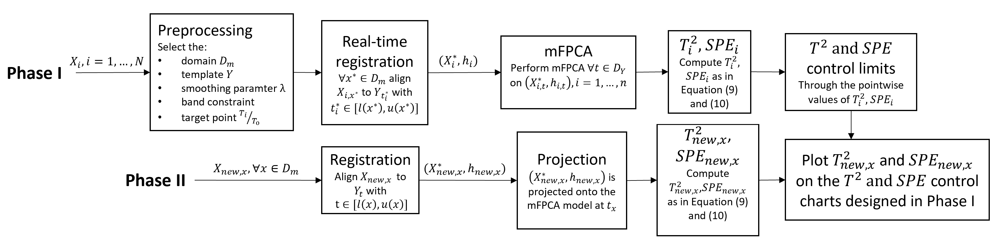
Figure 1: Scheme of FRTM approach.

2.4.1 Phase I

In this phase, a reference sample denoted by $X_{i}$, $i=1,\dots,N$, is used to characterize the IC operating conditions of the process.

A preprocessing step is needed to choose the common monitoring domain $\mathcal{D}_{m}$, as the compact interval over which the assessment of the process conditions could be of interest. Moreover, based on the domains $\mathcal{D}_{X_{i}}$ of the IC sample, $\mathcal{D}_{m}$ must be included in $\cup_{i=1}^{N}\mathcal{D}_{X_{i}}$, which implies at least one observation $X_{i}$ is defined for each $x\in\mathcal{D}_{m}$. Reasonably, $\mathcal{D}_{m}$ could be set as $\cup_{i=1}^{N}\mathcal{D}_{X_{i}}$. However, different choices could be driven by the specific application. The Procrustes fitting process and the $ACD$ approach described in Section 2.1 are used to identify an appropriate template function $Y$ and an appropriate value of the smoothing parameter $\lambda$. The subsequent real-time registration step considers a band constraint, applied to the terminal points of the partial warping functions and avoids too extreme warping functions. The two extremes of the band are denoted by $u,l:\mathcal{D}_{m}\rightarrow\mathcal{D}_{Y}$ and selected as the $(1-b/2)$ and $(b/2)$ pointwise quantiles, $b\in\left[0,1\right]$, of the warping functions obtained on the completely observed functional data. Note that, the band constraint serves also to set the maximum mismatch allowed range at the beginning and the end of the template function domain $\mathcal{D}_{Y}$ (as shown in Supplementary Materials A.1). Moreover, the target point $T_{i}/T_{0}$ in Equation (2) could be updated by considering the mean slope of the warping functions corresponding to $X_{i}$, and avoid wrong alignments in the real-time registration step detailed below, especially in the first part of the process.

In the real-time registration step, the functional observations of the IC sample are registered to the template function as they would have been observed until a specific point in $\mathcal{D}_{m}$. Specifically, for each $x^{*}\in\mathcal{D}_{m}$, the partial functional observation up to $x^{*}$ is denoted by $X_{i,x^{*}}:\mathcal{D}_{X_{i,x^{*}}}\subseteq\mathcal{D}_{X_{i}}$, where $\mathcal{D}_{X_{i,x^{*}}}$ is a compact domain in $\mathbb{R}$ having the same $\mathcal{D}_{X_{i}}$ left boundary and right boundary equal to $x^{*}$. Each partial observation $X_{i,x^{*}}$ is aligned to the template function truncated at $t_{i}^{*}\in\left[l(x^{*}),u(x^{*})\right]\subset\mathcal{D}_{Y}$ and denoted by $Y_{t_{i}^{*}}$. The point $t_{i}^{*}$ is chosen such that the obtained warping function minimizes the right-hand term in Equation (2) over the interval $\left[l(x^{*}),u(x^{*})\right]$. In addition, we do not allow the partial warping function corresponding to $X_{i,x^{*}}$, denoted by $h_{i,x^{*}}$, to be open-end, i.e., $h_{i,x^{*}}(t_{i}^{*})=x^{*}$. In this setting partial matches could be indeed easily handled by a different choice of $t_{i}^{*}$. Open-end warping functions are allowed for $x^{*}$, such that $u(x^{*})$ is equal to the right boundary of $\mathcal{D}_{Y}$. The band constraint forces $h_{i,x^{*}}$ to be defined on a domain where the right boundary is inside the range $\left[l(x^{*}),u(x^{*})\right]$. However, this could be too restrictive, e.g., for the use in Phase II where curve dynamics may not be well represented by the IC sample, and cause wrong alignments. To limit this issue, we consider an adaptive band constraint. The naive idea is based on the conjecture that when the uncertainty of $h_{i,x^{*}}$ at the right domain boundary is sufficiently small for all $x^{*}$ values in a given portion of the domain, the available information up to $x^{*}$ provides a reliable curve registration and the band constraint can be relaxed. Details on the calculation of the adaptive band constraint are provided in Supplementary Materials A.3.

Once all the IC observations are aligned in real-time, they can be used to perform the mFPCA step, described in Section 2.2. For each $t\in\mathcal{D}_{Y}$, mFPCA is applied to the pairs $\left(X^{*}_{i,t},h_{i,t}\right)$, $i=1,\dots,N$, where both $X^{*}_{i,t}$ and $h_{i,t}$ are defined on the compact domain $\mathcal{D}_{Y,t}$, which has the same left boundary of $\mathcal{D}_{Y}$ and $t$ as right boundary. However, it may exist $i=1,\dots,N$ for which $\left(X^{*}_{i,t},h_{i,t}\right)$ is not available, because the real-time registration step does not directly provide aligned and warping functions defined on $\mathcal{D}_{Y,t}$. In this case, the pair $\left(X^{*}_{i,t_{g}},h_{i,t_{g}}\right)$ defined on the smallest $\mathcal{D}_{Y,t_{g}}\supset\mathcal{D}_{Y,t}$, truncated at $t$, is considered in place of $\left(X^{*}_{i,t},h_{i,t}\right)$.

In the last step, Hotelling’s $T^{2}$ and $SPE$ statistics are computed for each observation $i=1,\dots,N$ and each $x\in\mathcal{D}_{m}$. Specifically, for each $x\in\mathcal{D}_{m}$ the observation $X_{i,x}$, through the corresponding aligned and warping functions pair $(X^{*}_{i,t_{x}},h_{i,t_{x}})$ on $\mathcal{D}_{Y,t_{x}}$, is projected on the mFPCA model corresponding to $t_{x}$. Therefore, the values of $T^{2}_{i}$ and $SPE_{i}$ functions at $x$ are computed as described in Section 2.3. Control limits are obtained by considering the pointwise values of $T^{2}_{i}$ and $SPE_{i}$ defined on $\mathcal{D}_{m}$ for a given overall type I error probability $\alpha$. Note that this last step could be performed with a reference sample, referred to as tuning set, that is different from the one used in the mFPCA step. This possibly reduces possible overfitting issues and increases the monitoring performance of FRTM.

In practice, $X_{i}$, and so the partial functional data $X_{i,x^{*}}$, are usually observed through noisy discrete values, and functional observations are recovered through standard smoothing techniques.

2.4.2 Phase II

As in the traditional SPC, Phase II refers to the perspective monitoring of new observations, given a chosen reference sample in Phase I. Let $X_{new,x}$ denote a new observation $X_{new,x}$ of the quality characteristic observed until $x\in\mathcal{D}_{m}$. Then, as described in Section 2.4.1, we obtain the corresponding aligned and warping function pair $(X^{*}_{new,t_{x}},h_{new,t_{x}})$, by projecting it onto the mFPCA space corresponding to $t_{x}$, we compute the values of $T^{2}_{new}$ and $SPE_{new}$ at $x$ as described in Section 2.3. An alarm signal is issued if it exists a $x\in\mathcal{D}_{m}$ such that $T^{2}_{new}$ or $SPE_{new}$ violates the corresponding control limits. Note that, although $X_{new,x}$ can be defined also for $x\notin\mathcal{D}_{m}$, then $X_{new,x}$ is monitored at $x\in\mathcal{D}_{m}$ alone.

3 Simulation Study

An extensive Monte Carlo simulation study is performed to assess the performance of the proposed FRTM in identifying mean shifts of the quality characteristic caused by perturbations of the amplitude and phase components. The data generation process is inspired by the works of Wang and Gasser (1997); Gasser and Wang (1999) and is detailed in Supplementary Materials B. Two different scenarios are considered and characterized by different phase components. Specifically, Scenario 1 considers simple quadratic warping functions, whereas Scenario 2 investigates a more complex temporal dynamics. Each scenario explores three models with decreasing levels of misalignment, quantified through the ratio between amplitude and phase variation and indicated through M1, M2, and M3. A Low level of misalignment corresponds to small values of phase variation and mimics e.g., those settings where a coarse registration is preliminarily applied to the data. Three different types of OC conditions are analysed and correspond to mean shifts affecting the phase component alone (Shift A), the amplitude component alone (Shift B) and both components simultaneously (Shift C). For each shift 4 different severity levels $d\in\{0.25,0.50,0.75,1.00\}$ are explored, as well as to mimic real-time monitoring OC scenarios, we simulate change points at 30% and 60% of the total duration of the process used to generate the data. As results are analogous for both change point scenarios, in this section, we present only the former case, whereas the latter is presented in Supplementary Materials C.

FRTM method is compared with two simpler natural competing approaches, namely the monitoring in real-time with no alignment, referred to as NOAL, and the pointwise monitoring approach of the functional quality characteristic, referred to as PW. The NOAL approach is based on the approach presented in Capezza et al. (2020), where a dimensionality reduction based on functional principal components is followed by a monitoring strategy built on the $T^{2}$ and $SPE$ control charts. The PW approach belongs to the class of methods where a synthetic index for each curve is extracted to be used in a univariate control chart, where the pointwise value of the quality characteristic is monitored through a Shewhart-type control chart. FRTM is implemented as described in Section 2, the template function is obtained through the Procrustes fitting process with 2 iterations and a curve randomly chosen as initial estimate, $s^{min}$ and $s^{max}$ are set equal to 0.01 and 1000, respectively,, and the value of $\lambda$ in Equation (2) is chosen through the average curve distance (Equation (3)) with $\delta=0.01$. The band constraint is implemented with $b=0.01$. Moreover, in the mFPCA step, the number of retained principal components $L$ is chosen such that the retained principal components explain at least $90\%$ of the total variability. The empirical quantiles of $T^{2}$ and $SPE$ statistics are obtained via the kernel density estimation approach (Chou et al., 2001) with the Gaussian kernel, 1000 equally spaced points and bandwidth chosen by means of the methods in Sheather and Jones (1991). While data are observed through noisy discrete values, functional observations are obtained by considering the usual spline smoothing approach based on cubic B-splines and a roughness penalty on the second derivative (Ramsay, 2005). 50 simulation runs are performed for each scenario, misalignment level, shift type and severity level. Each run considers an IC sample of 500 observations, where one half is used in the mFPCA step, and the remaining are used as tuning set to compute the control limits. The Phase II sample is composed of 500 OC observations.

FRTM and the competing method performance are assessed by means of the true detection rate (TDR), which is the proportion of domain outside the control limits whilst the process is OC, and the false alarm rate (FAR), which is the proportion of domain outside the control limits whilst the process is IC. The FAR should be similar to the overall type I error probability $\alpha$ that is considered to obtain the control limits and, in this simulation study, is set equal to $0.05$, whereas the TDR should be as close to one as possible.

Figure 2 and Figure 3 display the mean FAR ($d=0$) or TDR ($d\neq 0$) for Scenario 1 and Scenario 2 respectively, as a function of the severity level $d$ plus/minus one standard error for each shift type and misalignment M1, M2 and M3. Note that, the mean FAR corresponding to IC in the first part of the process for $d\neq 0$ is not displayed here as it achieves values comparable to those achieved for $d=0$.

Figure 2: Mean FAR ($d=0$) or TDR ($d\neq 0$) plus/minus one standard error achieved by FRTM, NOAL and PW, for each shift type (Shift A, B and C) and increasing misalignment level (M1, M2 and M3) as a function of the severity level $d$ in Scenario 1.

M1
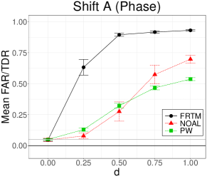
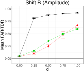
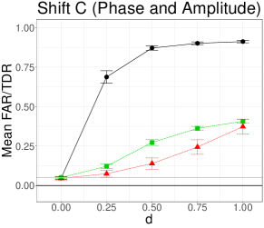
M2
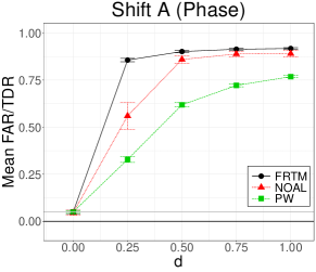
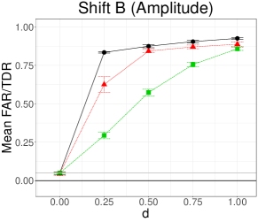
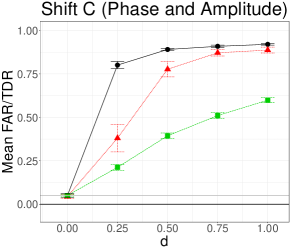
M3

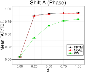
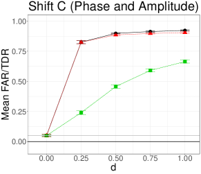
Figure 3: Mean FAR ($d=0$) or TDR ($d\neq 0$) plus/minus one standard error achieved by FRTM, NOAL and PW, for each shift type (Shift A, B and C) and increasing misalignment level (M1, M2 and M3) as a function of the severity level $d$ in Scenario 2.

M1
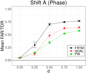
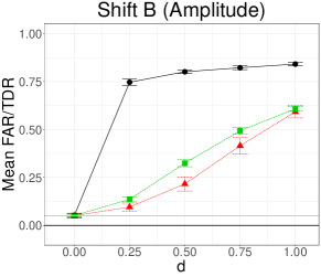
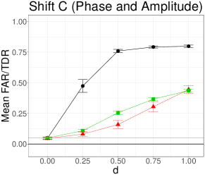
M2
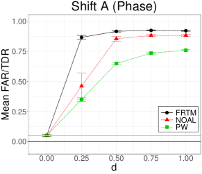
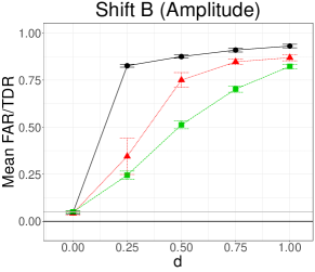
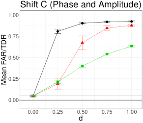
M3

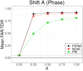
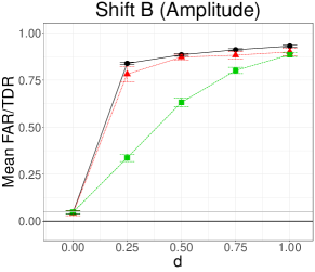
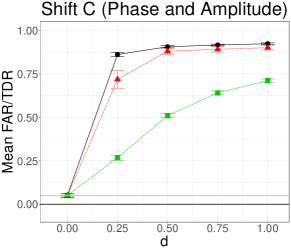
Figure 2 shows that all the methods successfully control the FAR in Scenario 1 and FRTM outperforms in terms of TDR both the NOAL and PW methods for all shift types and misalignments. As expected, the setting M1 with the largest phase variation is the most favourable for FRTM. In this case, for all types of shifts, FRTM outperforms the competing methods. The NOAL method is badly affected by large phase variation by showing particularly low detection rate performance, which is even comparable to that of the PW method. This comes from the fact that phase variation considerably influences the FPCA step of the NOAL method by masking the presence of OC conditions. On the contrary, FRTM is able to successfully deal with the function misalignment by separating phase and amplitude components and considering both sources of variability in the monitoring procedure. However, the performance difference between FRTM and the NOAL method decreases as the amplitude variation dominates the data variability. The NOAL method shows higher performance for misalignment M2 (i.e., mild amplitude/phase variation ratio) and TDR comparable with FRTM for misalignment M3 (i.e., low amplitude/phase variation ratio). It is interesting to note that the performance of FRTM is only slightly affected by the size of the phase variation, especially for large severity levels. This is particularly true for Shift B, where FRTM performance is almost the same for misalignment M1, M2, and M3. Moreover, for low values of misalignment, the higher complexity of FRTM method is not reflected in a lower OC detection performance, which emphasizes the ability of FRTM to deal with a wide range of phase variation scenarios.

As noted in Figure 3, also in Scenario 2, where the data are generated with more complex phase components, FRTM performance is much higher than that of the competing methods. However, the greater complexity of the phase component is reflected in a slightly lower detection power of FRTM, mainly for misalignment M1. Indeed, in Scenario 2, the largest mean TDRs achieved by FRTM correspond to Shift B and Shift C, where OC condition affects the amplitude component. Whereas, for Shift A, where the OC condition arises in the phase component alone, FRTM does not achieve as good performance as in Scenario 1. The ability of FRTM to successfully separate and then, combine the amplitude and phase components makes it the best performing real-time monitoring scheme for all the considered settings.

4 Data Example: Batch Monitoring of a Penicillin Production Process

To demonstrate the potential of FRTM in practical situations, in this section, we present an example that addresses the issue of monitoring batches from a penicillin production process. Batch processes play an important role in the production and processing of high-quality speciality materials and products that appear in the manufacturing, food and medicine industries among others (Nomikos and MacGregor, 1995a, b; Spooner et al., 2017; Spooner and Kulahci, 2018). A batch process is a finite-duration process where quantities of raw materials are subjected to a sequence of steps and conditions that transform them into the final product. Abnormal conditions that develop during these operations can lead to poor quality production. Therefore, real-time SPC can be successfully employed to detect and indicate OC conditions that can be possibly corrected prior to the batch completion.

The study considers the extensive dataset provided by Van Impe and Gins (2015), generated from the morphological model of Birol et al. (2002b) for the penicillin production in fed-batch cultivations. It describes the growth of biomass and production of penicillin in a fed-batch reactor, where the fermentation is operated in both batch and fed-batch modes. Further details about the penicillin production process can be found in Birol et al. (2002a, b). Specifically, we focus on four datasets, named D1, D2, D3 and D4, that represent different assumptions about the production process. D1 represents the basic case where all initial conditions are well modeled by a normal distribution. D2 considers other non-Gaussian distributions for the initial conditions. D3 includes also a batch-to-batch variation of the model parameters in addition to non-Gaussian initial conditions. Finally, D4 is similar to D3 with the added complexity of multi-modality due to two different strains in the simulation. Each dataset consists of 400 NOC batches and several thousand faulty batches where many variables are measured online every 12 minutes throughout each batch. In this example, we focus on the monitoring of two quality characteristics in real-time that are representative of the process state, considered in the first 100 hours of production; namely, the dissolved O₂ concentration, indicated with O₂ and measured in $mg/L$, and the base flow rate, indicated with BFR and measured in $mL/h$. In Supplementary Materials D, the plot of 400 IC observations of these two quality characteristics is shown for each dataset, where the presence of a significant proportion of phase variation is highlighted. Therefore, we expect FRTM to perform better than the NOAL method, which has been shown in Section 3 to be particularly sensitive to the presence of phase variation. The faulty batches consist of 15 different fault types, each with different fault magnitudes representative of a wide range of OC states (see Van Impe and Gins (2015) for further details on fault types). Specifically, 50 repetitions of each dataset/type/magnitude combination are available for a total of 3000 faulty batches, where the onset times of the OC conditions arise randomly during the process. FRTM is implemented as in Section 3, with $s^{min}=1$, $s^{max}=1000$, and the value of $\lambda$ in Equation (2) chosen through the average curve distance (Equation (3)) with $\delta=0.05$. The band constraint is implemented with $b=0.01$ and a number of retained principal components $L$ that explains at least $90\%$ of the total variability. Moreover, the empirical quantile of the $T^{2}$ and $SPE$ statistics are obtained via the kernel density estimation approach. As in the simulation study in Section 3, $\alpha$ is set equal to $0.05$.

In Figure 4, the mean TDR of FRTM and the competing methods applied to the O₂ and the BFR (row-wise) are plotted against the 15 fault types for each dataset (column-wise). Note that the mean TDR at each fault type is obtained by averaging across all fault magnitudes. Although the FDR is not explicitly shown here, we confirm that all methods achieve values that are close to nominal $\alpha$. Thus, they can be fairly compared in terms of TDR.

Figure 4: Mean TDR over the different fault magnitudes against fault type (1-15) achieved by FRTM, NOAL and PW for the O₂ and the BFR for each dataset (D1, D2, D3, and D4).

O2
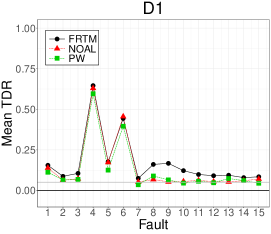
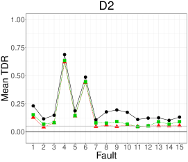
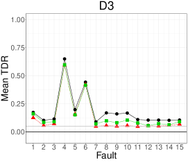
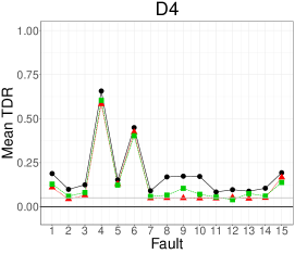
BFR

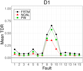
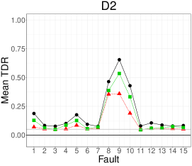
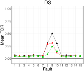
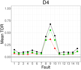
FRTM achieves the largest mean TDR for almost all the considered settings. Specifically, in the monitoring of O₂, FRTM outperforms competitors in detecting faults 1-3 and 7-15 that produce moderate values of TDR. This behaviour reflects the fact that FRTM is more inclined to detect small OC conditions than the PW method, due to its functional nature able to account for the whole curve pattern. The NOAL method, which should also have benefited from its functional nature, in this setting is badly affected by the presence of phase variation and, thus, shows worse performance than FRTM. For faults 4-6, the performance of FRTM and the competing methods are more similar even though the former is always the best one. The performance of the three methods slightly changes from D1 to D4. In the monitoring of the BFR, the considered methods show the largest mean TDR for faults 8-10. Also in this case, the NOAL method is particularly affected by the presence of phase variation. For faults 1-7 and 11-15, which represent OC conditions of moderate intensity, FRTM achieves the best performance.

For illustrative purposes, Figure 5 reports the application of the considered methods to monitor five batches randomly sampled from the quality characteristic BFR of the dataset D4. Also in this case, the mean TDR of FRTM is definitely larger than that of the NOAL and PW methods and confirms the results of Figure 4. As an example, by looking at the third observation, we clearly see that FRTM signals the OC condition much earlier than the competing methods.

Figure 5: $T_{2}$ and $SPE$ control charts based on FRTM and NOAL methods, and the PW control chart corresponding to five batches randomly sampled from the quality characteristic BFR of the dataset D4. The thick solid lines correspond to control limits.

FRTM	NOAL	PW

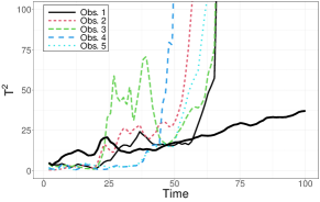
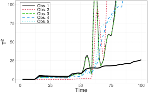
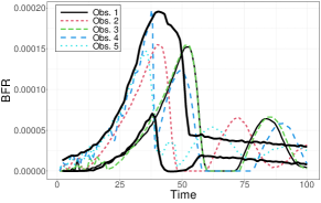
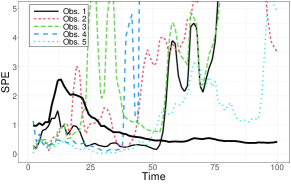
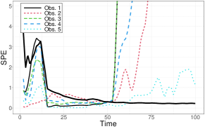
5 Conclusions

In this paper, we propose a new method for monitoring a functional quality characteristic in real-time, referred to as functional real-time monitoring (FRTM). FRTM is designed to assess the presence of assignable causes of variation before the process completion by taking into account both the phase and amplitude sources of variation. For instance, this could be of interest for long and expensive processes. Specifically, FRTM is based on three main elements: a curve registration based on an open-end/open-begin version of the functional dynamic time warping, a dimensionality reduction through a new version of the mixed functional principal component analysis, and a monitoring strategy based on Hotelling’s $T^{2}$ and $SPE$ control charts. To the best of the authors’ knowledge, FRTM is the first monitoring scheme that is able to monitor a functional quality characteristic in real-time by successfully combining the information in both the amplitude and phase components. Indeed, methods already present in the literature either skip the registration step overlooking the phase component or consider the phase variability as a nuisance effect to be removed. Both approaches have drawbacks, with the former risking producing low power procedures because phase variation could mask the true data structure, while the latter may not be able to account for OC conditions that arise in the phase component.

The performance of FRTM is assessed through an extensive Monte Carlo simulation study where it is compared with two competing real-time monitoring methods, named NOAL and PW, which overlook the presence of phase variation and the functional nature of the quality characteristics, respectively. Conversely, the ability of the proposed method to firstly separate and then combine amplitude and phase variations bring FRTM to outperform competitors in all considered scenarios, which covered a variety of types of phase components and OC conditions. Lastly, the practical applicability of the proposed method is illustrated through a data example, which addresses the issue of monitoring batches from a penicillin production process. Also in this case, FRTM shows better performance than the competitors in the identification of OC condition of the dissolved O₂ concentration, and the base flow rate.

Future research could be performed to extend the proposed framework to the case of multivariate functional data, which poses non trivial challenges from both computational and methodological points of view. To further improve the detection power of FRTM, the uncertainty in the estimation of the warping components could be included in the dimensionality reduction phase and an optimality criterion could be developed to better choose the weights in the mFPCA.

Supplementary Materials

Supplementary Materials contain additional details about the proposed method (A.1-A.3), details about the data generation process in the simulation study (B), additional simulation results (C), and additional plots for the data example (D), as well as the R code to reproduce graphics and results over competing methods in the simulation study.

References

- Birol et al. (2002a) Birol, G., C. Ündey, and A. Cinar (2002a). A modular simulation package for fed-batch fermentation: penicillin production. Computers & chemical engineering 26(11), 1553–1565.
- Birol et al. (2002b) Birol, G., C. Ündey, S. J. Parulekar, and A. Cinar (2002b). A morphologically structured model for penicillin production. Biotechnology and bioengineering 77(5), 538–552.
- Capezza et al. (2020) Capezza, C., A. Lepore, A. Menafoglio, B. Palumbo, and S. Vantini (2020). Control charts for monitoring ship operating conditions and co2 emissions based on scalar-on-function regression. Applied Stochastic Models in Business and Industry 36(3), 477–500.
- Centofanti et al. (2020) Centofanti, F., A. Lepore, A. Menafoglio, B. Palumbo, and S. Vantini (2020). Functional regression control chart. Technometrics, 1–14.
- Chou et al. (2001) Chou, Y.-M., R. L. Mason, and J. C. Young (2001). The control chart for individual observations from a multivariate non-normal distribution. Communications in statistics-Theory and methods 30(8-9), 1937–1949.
- Colosimo and Pacella (2007) Colosimo, B. M. and M. Pacella (2007). On the use of principal component analysis to identify systematic patterns in roundness profiles. Quality and reliability engineering international 23(6), 707–725.
- Ferraty and Vieu (2006) Ferraty, F. and P. Vieu (2006). Nonparametric functional data analysis: theory and practice. Springer Science & Business Media.
- Gasser and Kneip (1995) Gasser, T. and A. Kneip (1995). Searching for structure in curve samples. Journal of the american statistical association 90(432), 1179–1188.
- Gasser and Wang (1999) Gasser, T. and K. Wang (1999). Synchronizing sample curves nonparametrically. The Annals of Statistics 27(2), 439–460.
- González-Martínez et al. (2014) González-Martínez, J. M., O. E. de Noord, and A. Ferrer (2014). Multisynchro: a novel approach for batch synchronization in scenarios of multiple asynchronisms. Journal of Chemometrics 28(5), 462–475.
- González-Martínez et al. (2011) González-Martínez, J. M., A. Ferrer, and J. A. Westerhuis (2011). Real-time synchronization of batch trajectories for on-line multivariate statistical process control using dynamic time warping. Chemometrics and Intelligent Laboratory Systems 105(2), 195–206.
- Grasso et al. (2017) Grasso, M., B. M. Colosimo, and F. Tsung (2017). A phase i multi-modelling approach for profile monitoring of signal data. International Journal of Production Research 55(15), 4354–4377.
- Grasso et al. (2016) Grasso, M., A. Menafoglio, B. M. Colosimo, and P. Secchi (2016). Using curve-registration information for profile monitoring. Journal of Quality Technology 48(2), 99.
- Hadjipantelis et al. (2015) Hadjipantelis, P. Z., J. A. Aston, H.-G. Müller, and J. P. Evans (2015). Unifying amplitude and phase analysis: A compositional data approach to functional multivariate mixed-effects modeling of mandarin chinese. Journal of the American Statistical Association 110(510), 545–559.
- Happ (2017) Happ, C. (2017). MFPCA: Multivariate Functional Principal Component Analysis for Data Observed on Different Dimensional Domains. R package version 1.1.
- Happ and Greven (2018) Happ, C. and S. Greven (2018). Multivariate functional principal component analysis for data observed on different (dimensional) domains. Journal of the American Statistical Association, 1–11.
- Happ et al. (2019) Happ, C., F. Scheipl, A.-A. Gabriel, and S. Greven (2019). A general framework for multivariate functional principal component analysis of amplitude and phase variation. Stat 8(1), e220.
- Horváth and Kokoszka (2012) Horváth, L. and P. Kokoszka (2012). Inference for functional data with applications. Springer Science & Business Media.
- Hron et al. (2016) Hron, K., A. Menafoglio, M. Templ, K. Hrŭzová, and P. Filzmoser (2016). Simplicial principal component analysis for density functions in bayes spaces. Computational Statistics & Data Analysis 94, 330–350.
- Itakura (1975) Itakura, F. (1975). Minimum prediction residual principle applied to speech recognition. IEEE Transactions on acoustics, speech, and signal processing 23(1), 67–72.
- James (2007) James, G. M. (2007). Curve alignment by moments. The Annals of Applied Statistics 1(2), 480–501.
- Jolliffe (2011) Jolliffe, I. (2011). Principal component analysis. Springer.
- Kassidas et al. (1998) Kassidas, A., J. F. MacGregor, and P. A. Taylor (1998). Synchronization of batch trajectories using dynamic time warping. AIChE Journal 44(4), 864–875.
- Kneip and Gasser (1992) Kneip, A. and T. Gasser (1992). Statistical tools to analyze data representing a sample of curves. The Annals of Statistics, 1266–1305.
- Kokoszka and Reimherr (2017) Kokoszka, P. and M. Reimherr (2017). Introduction to functional data analysis. Chapman and Hall/CRC.
- Lee and Jung (2016) Lee, S. and S. Jung (2016). Combined analysis of amplitude and phase variations in functional data. arXiv preprint arXiv:1603.01775.
- Lehmann and Romano (2006) Lehmann, E. L. and J. P. Romano (2006). Testing statistical hypotheses. Springer Science & Business Media.
- Marron et al. (2014) Marron, J., J. O. Ramsay, L. M. Sangalli, and A. Srivastava (2014). Statistics of time warpings and phase variations. Electronic Journal of Statistics 8(2), 1697–1702.
- Marron et al. (2015) Marron, J. S., J. O. Ramsay, L. M. Sangalli, and A. Srivastava (2015). Functional data analysis of amplitude and phase variation. Statistical Science, 468–484.
- Menafoglio et al. (2018) Menafoglio, A., M. Grasso, P. Secchi, and B. M. Colosimo (2018). Profile monitoring of probability density functions via simplicial functional pca with application to image data. Technometrics 60(4), 497–510.
- Montgomery (2007) Montgomery, D. C. (2007). Introduction to statistical quality control. John Wiley & Sons.
- Mosesova et al. (2006) Mosesova, S. A., H. A. Chipman, R. J. MacKay, and S. H. Steiner (2006). Profile monitoring using mixed-effects models. Dept. Statist. Actuarial Sci., Univ. Waterloo, Waterloo, ON, Canada, Tech. Rep, 06–06.
- Nomikos and MacGregor (1995a) Nomikos, P. and J. F. MacGregor (1995a). Multi-way partial least squares in monitoring batch processes. Chemometrics and intelligent laboratory systems 30(1), 97–108.
- Nomikos and MacGregor (1995b) Nomikos, P. and J. F. MacGregor (1995b). Multivariate spc charts for monitoring batch processes. Technometrics 37(1), 41–59.
- Noorossana et al. (2012) Noorossana, R., A. Saghaei, and A. Amiri (2012). Statistical analysis of profile monitoring. John Wiley & Sons.
- Pini et al. (2017) Pini, A., S. Vantini, B. M. Colosimo, and M. Grasso (2017). Domain-selective functional analysis of variance for supervised statistical profile monitoring of signal data. Journal of the Royal Statistical Society: Series C (Applied Statistics).
- R Core Team (2021) R Core Team (2021). R: A Language and Environment for Statistical Computing. Vienna, Austria: R Foundation for Statistical Computing.
- Ramsay (2005) Ramsay, J. O. (2005). Functional data analysis. Wiley Online Library.
- Ramsay and Dalzell (1991) Ramsay, J. O. and C. Dalzell (1991). Some tools for functional data analysis. Journal of the Royal Statistical Society. Series B (Methodological) 53(3), 539–572.
- Ramsay and Li (1998) Ramsay, J. O. and X. Li (1998). Curve registration. Journal of the Royal Statistical Society: Series B (Statistical Methodology) 60(2), 351–363.
- Sakoe and Chiba (1978) Sakoe, H. and S. Chiba (1978). Dynamic programming algorithm optimization for spoken word recognition. IEEE transactions on acoustics, speech, and signal processing 26(1), 43–49.
- Shallom et al. (1989) Shallom, I. D., R. Haimi-Cohen, and T. Golan (1989). Dynamic time warping with boundaries constraint relaxation. In The Sixteenth Conference of Electrical and Electronics Engineers in Israel,, pp. 1–4. IEEE.
- Sheather and Jones (1991) Sheather, S. J. and M. C. Jones (1991). A reliable data-based bandwidth selection method for kernel density estimation. Journal of the Royal Statistical Society. Series B (Methodological) 53(3), 683–690.
- Silverman (1995) Silverman, B. W. (1995). Incorporating parametric effects into functional principal components analysis. Journal of the Royal Statistical Society: Series B (Methodological) 57(4), 673–689.
- Spooner et al. (2017) Spooner, M., D. Kold, and M. Kulahci (2017). Selecting local constraint for alignment of batch process data with dynamic time warping. Chemometrics and Intelligent Laboratory Systems 167, 161–170.
- Spooner and Kulahci (2018) Spooner, M. and M. Kulahci (2018). Monitoring batch processes with dynamic time warping and k-nearest neighbours. Chemometrics and Intelligent Laboratory Systems 183, 102–112.
- Srivastava et al. (2011) Srivastava, A., W. Wu, S. Kurtek, E. Klassen, and J. S. Marron (2011). Registration of functional data using fisher-rao metric. arXiv preprint arXiv:1103.3817.
- Tormene et al. (2009) Tormene, P., T. Giorgino, S. Quaglini, and M. Stefanelli (2009). Matching incomplete time series with dynamic time warping: an algorithm and an application to post-stroke rehabilitation. Artificial intelligence in medicine 45(1), 11–34.
- Van Impe and Gins (2015) Van Impe, J. and G. Gins (2015). An extensive reference dataset for fault detection and identification in batch processes. Chemometrics and Intelligent Laboratory Systems 148, 20–31.
- Wang and Gasser (1997) Wang, K. and T. Gasser (1997). Alignment of curves by dynamic time warping. The annals of Statistics 25(3), 1251–1276.
- Wold et al. (1998) Wold, S., N. Kettaneh, H. Fridén, and A. Holmberg (1998). Modelling and diagnostics of batch processes and analogous kinetic experiments. Chemometrics and intelligent laboratory systems 44(1-2), 331–340.
- Woodall et al. (2004) Woodall, W. H., D. J. Spitzner, D. C. Montgomery, and S. Gupta (2004). Using control charts to monitor process and product quality profiles. Journal of Quality Technology 36(3), 309.