Graph Fourier transform based on singular value decomposition of directed Laplacian

Abstract

Graph Fourier transform (GFT) is a fundamental concept in graph signal processing. In this paper, based on singular value decomposition of Laplacian, we introduce a novel definition of GFT on directed graphs, and use singular values of Laplacian to carry the notion of graph frequencies. The proposed GFT is consistent with the conventional GFT in the undirected graph setting, and on directed circulant graphs, the proposed GFT is the classical discrete Fourier transform, up to some rotation, permutation and phase adjustment. We show that frequencies and frequency components of the proposed GFT can be evaluated by solving some constrained minimization problems with low computational cost. Numerical demonstrations indicate that the proposed GFT could represent graph signals with different modes of variation efficiently.

I Introduction

Graph signal processing provides an innovative framework to represent, analyze and process data sets residing on networks, and its mathematical foundation is closely related to applied and computational harmonic analysis and spectral graph theory [1]-[8]. Graph Fourier transform (GFT) is one of fundamental tools in graph signal processing that decomposes graph signals into different frequency components and represents them by different modes of variation. GFT on directed graphs is an important tool to identify patterns and quantify influence of various members and communities of a social network, and to understand dynamic of a network. The GFT on undirected graphs has been well-studied and several approaches have been proposed to define GFT on directed graphs [3, 7, 9]-[20]. In this paper, we introduce a novel definition of GFT on directed graphs, which is based on singular value decomposition of the associated Laplacian, see Definition II.1.

Let ${\mathcal{G}}=(V,E)$ be a weighted (un)directed graph of order $N$ containing no loops or multiple edges, and denote the associated adjacency matrix, in-degree matrix and Laplacian by ${\bf A},{\bf D}$ and ${\bf L}:={\bf D}-{\bf A}$ respectively. In the undirected graph setting (i.e., the associated adjacent matrix ${\bf A}$ is symmetric), the Laplacian ${\mathbf{L}}$ is positive semi-definite and it has the following eigendecomposition

$${\bf L}={\bf V}{\boldsymbol{\Lambda}}{\bf V}^{T}=\sum_{i=0}^{N-1}\lambda_{i}{\bf v}_{i}{\bf v}_{i}^{T},$$ (I.1)

where ${\bf V}=[{\bf v}_{0},\ldots,{\bf v}_{N-1}]$ is an orthogonal matrix and ${\boldsymbol{\Lambda}}={\rm diag}(\lambda_{0},\ldots,\lambda_{N-1})$ is a diagonal matrix of nonnegative eigenvalues of the Laplacian ${\mathbf{L}}$ in nondecreasing order, i.e., $\lambda_{0}\leq\ldots\leq\lambda_{N-1}$. A well-accepted definition of GFT in the undirected graph setting is given by

$${\mathcal{F}}{\bf x}={\bf V}^{T}{\bf x}=\sum_{i=0}^{N-1}\langle{\bf x},{\bf v}_{i}\rangle{\bf v}_{i},$$ (I.2)

where ${\bf x}$ is a graph signal and $\langle\cdot,\cdot\rangle$ is the standard inner product on ${\mathbb{R}}^{N}$ [6, 7, 9, 18, 20, 21]. The eigenvalues $\lambda_{i}$ and the associated eigenvectors ${\bf v}_{i},0\leq i\leq N-1$, of the Laplacian ${\mathbf{L}}$ are considered as frequencies and frequency components of the GFT just defined. It is known that the GFT in (I.2) is orthogonal and on a cycle graph, it is essentially the classical discrete Fourier transform.

The GFT (I.2) does not apply directly for weighted and directed graphs, which are widely used to describe the interaction structure of a social network that has members of various types, such as individuals, organizations, leaders and followers, and the pairwise interactions between members being not always mutual and equitable [22]-[24]. A natural approach is to replace the eigendecomposition (I.1) of the Laplacian ${\mathbf{L}}$ by the Jordan decomposition ${\bf L}={\bf V}{\bf J}{\bf V}^{-1}$, and then to define the GFT of a signal ${\bf x}$ on a directed graph by

$${\cal F}{{\bf x}}={\bf V}^{-1}{{\bf x}}$$ (I.3)

[3, 10, 11, 12, 14, 19]. The GFT in (I.3) could have complex frequencies and it is not always unitary. More critically, Jordan decomposition of the Laplacian ${\mathbf{L}}$ on directed graphs could be numerically unstable and computationally expensive, and hence it could be difficult to be applied for graph spectral analysis and decomposition, see [19] for a modified Jordan decomposition with some numerical stability. Our GFT in Definition II.1 is based on the singular value decomposition (SVD)

$${\bf L}={\bf U}\boldsymbol{\Sigma}{\bf V}^{T}=\sum_{i=0}^{N-1}\sigma_{i}{\bf u}_{i}{\bf v}_{i}^{T}$$ (I.4)

of the Laplacian ${\bf L}$ and has its nonnegative singular values $\sigma_{i},0\leq i\leq N-1$, as frequencies and ${\bf u}_{i},{\bf v}_{i},0\leq i\leq N-1$ as the associated left/right frequency components, where

$${\bf U}=[{\bf u}_{0},\ldots,{\bf u}_{N-1}]\ {\rm and}\ {\bf V}=[{\bf v}_{0},\ldots,{\bf v}_{N-1}]$$ (I.5)

are orthogonal matrices, and the diagonal matrix $\boldsymbol{\Sigma}={\rm diag}(\sigma_{0},\ldots,\sigma_{N-1})$ has singular values deployed on the diagonal in a nondecreasing order, i.e., $0\leq\sigma_{0}\leq\sigma_{1}\leq\ldots\leq\sigma_{N-1}$. Compared with the GFT (I.3) based on a Jordan decomposition, a significant advantage of the proposed SVD-based GFT is on numerically stability and low computational cost.

Given a graph signal ${\bf x}$ on a directed graph, denote its Euclidean norm by $\|{\bf x}\|_{2}$, and define its quadratic variation by

$${\rm QV}({\bf x})={\bf x}^{T}{\bf L}{\bf x}=\frac{1}{2}{\bf x}^{T}({\bf L}+{\bf L}^{T}){\bf x}$$ (I.6)

[6, 7, 9, 15]. In the undirected graph setting, frequencies $\lambda_{i}$ and their corresponding frequency components ${\bf v}_{i},0\leq i\leq N-1$, of the GFT in (I.2) can be obtained via solving the following constrained minimization problems

$$\left\{\begin{array}[]{l}\lambda_{i}=\min_{{\bf x}\in W_{i}^{\perp}\ {\rm with}\ \|{\bf x}\|_{2}=1}{\rm QV}({\bf x})\\ {\bf v}_{i}=\arg\min_{{\bf x}\in W_{i}^{\perp}\ {\rm with}\ \|{\bf x}\|_{2}=1}{\rm QV}({\bf x})\end{array}\right.$$ (I.7)

inductively for $1\leq i\leq N-1$, where $\lambda_{0}=0$, the initial ${\bf v}_{0}$ is usually selected by $N^{-1/2}{\bf 1}$, and $W_{i}^{\perp},1\leq i\leq N-1$, are the orthogonal complements of the space spanned by ${\bf v}_{j},0\leq j\leq i-1$. We remark that the quadratic variation $\rm QV$ in (I.6) overlook the edge direction in the directed graph setting. To define GFT on directed graphs, several directed variations to measure the change of signals along the graph structure have been proposed [13, 15, 16]. The authors in [13, 15, 16] define frequency and frequency components of GFT on directed graphs via solving some constrained optimization problems with directed variations as their objective functions, see Remark III.1 for detailed explanation. In Section III, we show that right frequency components ${\bf v}_{i},0\leq i\leq N-1$, of the proposed GFT can be obtained via solving constrained minimization problems (I.7) with the objective function ${\rm QV}({\bf x})$ replaced by $\|{\bf L}{\bf x}\|_{2}=\sqrt{{\bf x}^{T}{\bf L}^{T}{\bf L}{\bf x}}$, see (III.8). Compared with the GFTs based on constrained optimization of directed variations in [13] and [16], major differences are that the GFT proposed in this paper coincides with the conventional GFT (I.2) in the undirected graph setting, see (II.10), and that on directed circulant graphs, it is essentially the classical discrete Fourier transform, up to certain rotation, permutation and phase adjustment, see Theorem II.2.

We say that a graph ${\mathcal{E}}$ is an Eulerian graph if the in-degree and out-degree are the same at each vertex, and that ${\mathcal{E}}^{T}$ is the transpose of a directed graph ${\mathcal{E}}$ if they have the same vertex set and the adjacent matrix is the transpose of the adjacent matrix of the original graph ${\mathcal{E}}$. To measure the “symmetry” of a directed Eulerian graph ${\mathcal{E}}$, in Section IV we consider GFT ${\mathcal{F}}_{t},0\leq t\leq 1$, on a family of directed graphs ${\mathcal{E}}_{t},0\leq t\leq 1$, to connect an Eulerian graph ${\mathcal{E}}$ to its transpose ${\mathcal{E}}^{T}$, and study algebraic and analytic properties of the corresponding frequencies and frequency components of the GFT ${\mathcal{F}}_{t},0\leq t\leq 1$, see (IV.9), (IV.11), and Theorems IV.1, IV.2 and IV.3.

Notation: Bold lower cases and capitals are used to represent the column vectors and matrices respectively. Denote the Hermitian and transpose of a matrix ${\bf A}$ by ${\bf A}^{H}$ and ${\bf A}^{T}$ respectively, and use $\bf 1$, $\bf 0$, $\bf I$ and $\bf O$ to represent a vector with all 1s, a row/column vector with all 0s, an identity matrix, and a zero matrix of appropriate size.

II Graph Fourier transforms on directed graphs

Let ${\mathcal{G}}=(V,E)$ be a weighted directed graph of order $N$ containing no loops or multiple edges, and denote the associated Laplacian by ${\bf L}={\bf D}-{\bf A}$, where the adjacent matrix ${\bf A}=(a_{ij})_{i,j\in V}$ has nonzero weights $a_{ij}\neq 0$ only when there is an directed edge from node $j$ to node $i$, and the in-degree matrix ${\bf D}={\rm diag}(d_{i})_{i\in V}$ has the in-degree $d_{i}=\sum_{j\in V}a_{ij}$ of node $i\in V$ as its diagonal entries. The Laplacian ${\mathbf{L}}$ has eigenvalue zero and the constant signal ${\bf 1}$ as an associated eigenvector

$${\bf L}{\bf 1}={\bf 0},$$ (II.1)

and in the undirected graph setting, its eigendecomposition (I.1) is used to define GFT on undirected graphs [6, 7, 21]. In this section, based on the eigendecomposition (II.3) of the self-adjoint dilation ${\cal S}({\bf L})$ of the Laplacian ${\bf L}$, we propose a novel definition of GFT and inverse GFT on directed graphs, see Definition II.1. The proposed GFT preserves the Parseval identity, see (II.7), and in the undirected graph setting, it coincides with the conventional GFT in (I.2), see (II.10). Circulant graphs have been widely used in image processing [25]-[28]. In Theorem II.2, we show that the proposed SVD-based GFT on a directed circulant graph is essentially the classical discrete Fourier transform, up to certain rotation, permutation and phase adjustment.

Let orthogonal matrices ${\bf U}=[{\bf u}_{0},\ldots,{\bf u}_{N-1}],{\bf V}=[{\bf v}_{0},\ldots,{\bf v}_{N-1}]$ and diagonal matrix $\boldsymbol{\Sigma}={\rm diag}(\sigma_{0},\ldots,\sigma_{N-1})$ be as in the SVD (I.4) of the Laplacian ${\bf L}$. Then the self-adjoint dilation

$${\cal S}({\bf L}):=\begin{pmatrix}{\bf O}&{\bf L}\\ {\bf L}^{T}&{\bf O}\end{pmatrix}\in{\mathbb{R}}^{2N\times 2N}$$ (II.2)

of the Laplacian ${\bf L}$ has the following eigendecomposition,

$${\cal S}({\bf L})={\bf F}\begin{pmatrix}\boldsymbol{\Sigma}&{\bf O}\\ {\bf O}&-\boldsymbol{\Sigma}\end{pmatrix}{\bf F}^{T},$$ (II.3)

where

$${\bf F}=\frac{1}{\sqrt{2}}\begin{pmatrix}{\bf U}&{\bf U}\\ {\bf V}&-{\bf V}\end{pmatrix}\in{\mathbb{R}}^{2N\times 2N}$$ (II.4)

is an orthogonal matrix. Using the above orthogonal matrix ${\bf F}$, we define the GFT and inverse GFT on the directed graph ${\mathcal{G}}$ as follows.

Definition II.1.

Let ${\bf F}$ be the orthogonal matrix in (II.4). We define graph Fourier transform ${\mathcal{F}}:{\mathbb{R}}^{N}\longmapsto{\mathbb{R}}^{2N}$ and inverse graph Fourier transform ${\mathcal{F}}^{-1}:{\mathbb{R}}^{2N}\longmapsto{\mathbb{R}}^{N}$ on the directed graph ${\mathcal{G}}$ by

$$\mathcal{F}{\bf x}:={\bf F}^{T}\begin{pmatrix}{\bf x}/\sqrt{2}\\ {\bf x}/\sqrt{2}\end{pmatrix}=\begin{pmatrix}({\bf U}^{T}+{\bf V}^{T}){\bf x}/2\\ ({\bf U}^{T}-{\bf V}^{T}){\bf x}/2\end{pmatrix}$$ (II.5)

and

$${\mathcal{F}}^{-1}\begin{pmatrix}{\bf z}_{1}\\ {\bf z}_{2}\end{pmatrix}\hskip-2.168pt:=\hskip-3.61371pt\begin{pmatrix}\frac{{\bf I}}{\sqrt{2}}\ \frac{{\bf I}}{\sqrt{2}}\end{pmatrix}{\bf F}\begin{pmatrix}{\bf z}_{1}\\ {\bf z}_{2}\end{pmatrix}\hskip-2.168pt=\hskip-2.168pt\frac{1}{2}\big{(}{\bf U}({\bf z}_{1}+{\bf z}_{2})+{\bf V}({\bf z}_{1}-{\bf z}_{2})\big{)},\qquad$$ (II.6)

where ${\bf x}$ is a graph signal on ${\mathcal{G}}$ and ${\bf z}_{1},{\bf z}_{2}\in{\mathbb{R}}^{N}$.

The GFT in (II.5) provides a tool to analyze and represent signals in the spectral domain. Shown in Figure 1 is a piecewise constant signal on a weighted Minnesota traffic graph (left), the frequencies $\sigma_{i},0\leq i\leq N-1$, of the proposed GFT (second), and the first and next $N$-th components of the GFT of a piecewise constant signal on the graph (third and right). We observe that the piecewise constant signal on the weighted Minnesota graph has its energy concentrated mainly at low frequencies.

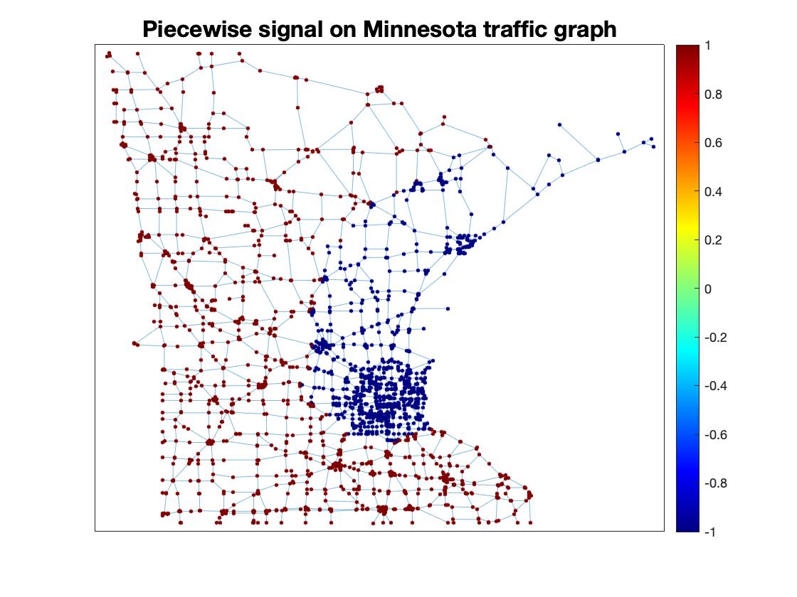
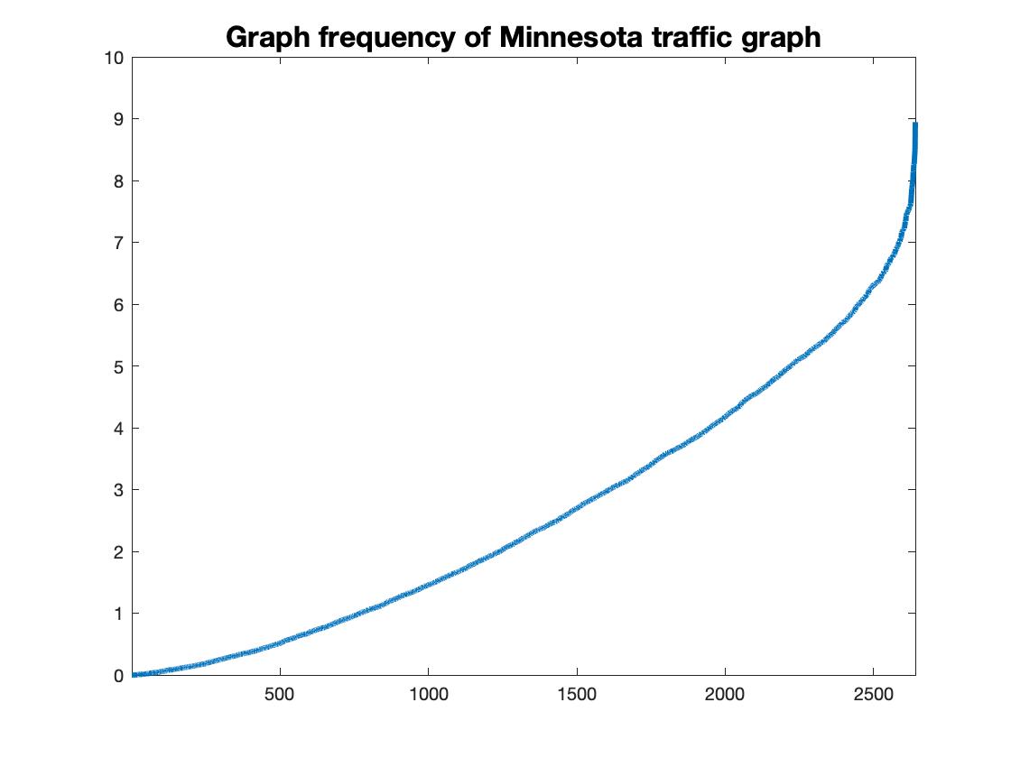
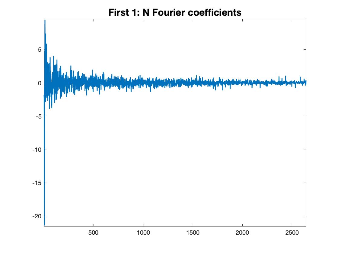
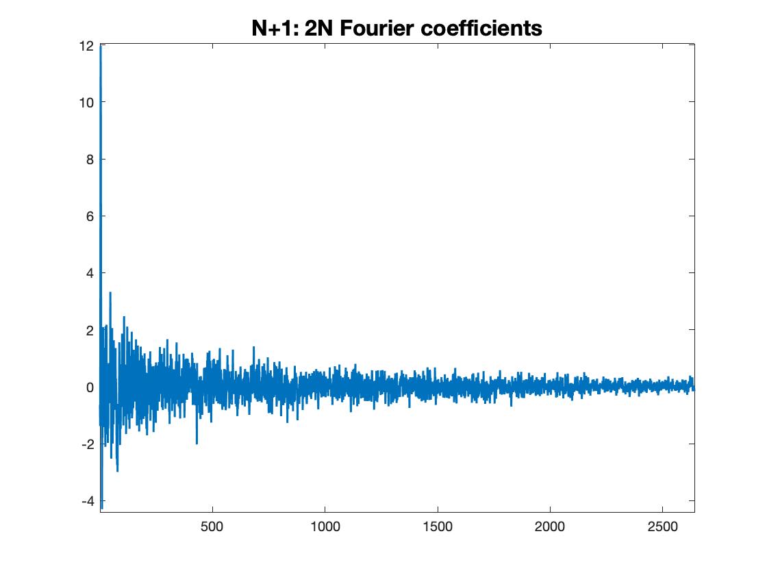
Figure 1: Plotted on the left and the second are a piecewise constant signal ${\bf x}_{0}$ on a weighted Minnesota traffic graph of order $N=2640$ with the weights $w_{ij}$ on adjacent edges $(j,i)$ being randomly chosen in the interval $[0,2]$, and the frequencies $\sigma_{i},0\leq i\leq N-1$, in (III.2) of our SVD-based GFT respectively. On the third and fourth are the first $N$-component $({\bf U}^{T}+{\bf V}^{T}){\bf x}_{0}/2$ and the next $N$-components $({\bf U}^{T}-{\bf V}^{T}){\bf x}_{0}/2$ of the GFT ${\mathcal{F}}{\bf x}_{0}$ of the signal ${\bf x}_{0}$ plotted on the left. The relative percentage of signal energy $(\sum_{i=0}^{M-1}|({\bf u}_{i}+{\bf v}_{i})^{T}{\bf x}_{0}/2|^{2}+|({\bf u}_{i}-{\bf v}_{i})^{T}{\bf x}_{0}/2|^{2})^{1/2}/\|{\bf x}_{0}\|_{2}$ for the first $M=20,50$ and $100$ frequencies are $0.6964,0.7602,0.8063$.

By the orthogonality of the matrix ${\bf F}$, one may verify that the Parseval’s identity holds,

$$\|{\bf x}\|_{2}=\|\mathcal{F}{\bf x}\|_{2},\ {\bf x}\in{\mathbb{R}}^{N},$$ (II.7)

and the inverse GFT ${\mathcal{F}}^{-1}$ is the pseudo-inverse of the GFT ${\mathcal{F}}$, i.e.,

$${\mathcal{F}}^{-1}\begin{pmatrix}{\bf z}_{1}\\ {\bf z}_{2}\end{pmatrix}={\rm arg}\min_{{\bf z}\in{\mathbb{R}}^{N}}\left\|{\mathcal{F}}{\bf z}-\begin{pmatrix}{\bf z}_{1}\\ {\bf z}_{2}\end{pmatrix}\right\|_{2},\ {\bf z}_{1},{\bf z}_{2}\in{\mathbb{R}}^{N}.$$ (II.8)

Therefore the original graph signal ${\bf x}$ can be reconstructed from its GFT ${\mathcal{F}}{\bf x}$,

$${\mathcal{F}}^{-1}{\mathcal{F}}{\bf x}={\bf x},\ \ {\bf x}\in{\mathbb{R}}^{N}.$$ (II.9)

For the case that the graph ${\mathcal{G}}$ is undirected, orthogonal matrices ${\bf U}$ and ${\bf V}$ in (I.4) can be selected to be the same, i.e., ${\bf U}={\bf V}$. Then the corresponding GFT ${\mathcal{F}}{\bf x}$ of a graph signal ${\bf x}$ becomes

$${\mathcal{F}}{\bf x}=\begin{pmatrix}{\bf V}^{T}{\bf x}\\ {\bf 0}\end{pmatrix}.$$ (II.10)

This shows that, in the undirected graph setting, the proposed SVD-based GFT is essentially the same as the well-accepted GFT (I.2) on undirected graphs.

For $N\geq 1$ and a set $Q=\{q_{1},\ldots,q_{L}\}$ of positive integers ordered with $1\leq q_{1}<\ldots<q_{L}\leq N-1$, let the directed circulant graph ${\mathcal{C}}_{d}:={\mathcal{C}}_{d}(N,Q)$ generated by $Q$ be the unweighted graph with the vertex set $V_{N}=\{0,1,\ldots,N-1\}$ and the edge set $E_{N}(Q)=\{(i,i+q\ {\rm mod}\ N),\ i\in V_{N},q\in Q\}$, where we say that $a=b\ {\rm mod}\ N$ if $(a-b)/N$ is an integer [25]-[28]. Set

$$P(z)=L-\sum_{l=1}^{L}z^{q_{l}},$$ (II.11)

and denote the discrete Fourier transform matrix by

$${\bf W}:=\big{(}N^{-1/2}\omega_{N}^{ij}\big{)}_{0\leq i,j\leq N-1},$$ (II.12)

where $\omega_{N}=\exp(2\pi\sqrt{-1}/N)$ is the $N$-th root of the unit. One may verify that the Laplacian ${\bf L}_{{\mathcal{C}}_{d}}$ on the directed circulant graph ${\mathcal{C}}_{d}$ is a circulant matrix that has eigenvalues

$$P(\omega_{N}^{i})=|P(\omega_{N}^{i})|\exp(\sqrt{-1}\theta_{i}),0\leq i\leq N-1,$$ (II.13)

and the $i$-th column of the discrete Fourier transform matrix ${\bf W}$ as an unit eigenvector associated with the eigenvalue $P(\omega_{N}^{i}),0\leq i\leq N-1$, where

$$\exp(\sqrt{-1}\theta_{i})=\left\{\begin{array}[]{ll}1&{\rm if}\ P(\omega_{N}^{i})=0\\ P(\omega_{N}^{i})/|P(\omega_{N}^{i})|&{\rm if}\ P(\omega_{N}^{i})\neq 0.\end{array}\right.$$

Let

$${\bf R}=\left\{\begin{array}[]{ll}{\rm diag}(1,{\bf R}_{2},\ldots,{\bf R}_{2})&{\rm if}\ N\ {\rm is\ odd}\\ {\rm diag}(1,{\bf R}_{2},\ldots,{\bf R}_{2},1)&{\rm if}\ N\ {\rm is\ even}\end{array}\right.$$ (II.14)

be the block diagonal matrix with number one and the $2\times 2$ unitary matrix ${\bf R}_{2}=\frac{1}{\sqrt{2}}\begin{pmatrix}1&-\sqrt{-1}\\ 1&\sqrt{-1}\end{pmatrix}$ as its diagonal blocks, and let the diagonal matrix

$${\bf\Theta}={\rm diag}\big{(}\exp(\sqrt{-1}\theta_{0}),\ldots,\exp(\sqrt{-1}\theta_{N-1})\big{)}$$ (II.15)

have phases $\exp(\sqrt{-1}\theta_{i})$ in (II.13) as its diagonal entries. In Proposition .1 of Appendix -A, we show that the Laplacian matrix ${\bf L}_{{\mathcal{C}}_{d}}$ on the directed circulant graph ${\mathcal{C}}_{d}$ has the following SVD,

$${\bf L}_{{\mathcal{C}}_{d}}={\bf U}{\boldsymbol{\Sigma}}{\bf V}^{T},$$ (II.16)

where ${\bf P}_{0}$ and ${\bf P}_{1}$ are permutation matrices (see (.6) and (.7) for explicit expressions),

$${\bf U}={\bf W}{\bf\Theta}{\bf P}_{0}{\bf R}{\bf P}_{1}\ {\rm and}\ {\bf V}={\bf W}{\bf P}_{0}{\bf R}{\bf P}_{1}$$ (II.17)

are orthogonal matrices with real entries, and

$${\boldsymbol{\Sigma}}={\rm diag}(\sigma_{0},\ldots,\sigma_{N-1})$$ (II.18)

has diagonal entries being nondecreasing rearrangement of the magnitudes $|P(\omega_{N}^{i})|,0\leq i\leq N-1$, in (II.13). Based on the above SVD of the Laplacian matrix ${\bf L}_{{\mathcal{C}}_{d}}$, we observe that the GFT in Definition II.1 is essentially the classical discrete Fourier transform,

$${\rm DFT}({\bf x}):={\bf W}^{H}{\bf x},\ {\bf x}\in{\mathbb{R}}^{N},$$ (II.19)

up to certain rotation ${\bf R}$, phase adjustment ${\bf\Theta}$ and permutations ${\bf P}_{0}$ and ${\bf P}_{1}$.

Theorem II.2.

Let $N\geq 1,Q=\{q_{1},\ldots,q_{L}\}$ be a set of positive integers with $1\leq q_{1}<\ldots<q_{L}\leq N-1$, ${\mathcal{C}}_{d}(N,Q)$ be the directed circulant graph generated by $Q$, and take the SVD (II.16) of the Laplacian matrix ${\bf L}_{{\mathcal{C}}_{d}}$ on ${\mathcal{C}}_{d}(N,Q)$. Then the corresponding GFT in (II.5) is given by

$${\mathcal{F}}{\bf x} \hskip-5.78172pt= \hskip-5.78172pt\frac{1}{2}\begin{pmatrix}{\bf P}_{1}&{\bf O}\\ {\bf O}&{\bf P}_{1}\end{pmatrix}\begin{pmatrix}{\bf R}&{\bf O}\\ {\bf O}&{\bf R}\end{pmatrix}^{H}\begin{pmatrix}{\bf P}_{0}&{\bf O}\\ {\bf O}&{\bf P}_{0}\end{pmatrix}\begin{pmatrix}{\bf\Theta}&{\bf\Theta}\\ {\bf I}&-{\bf I}\end{pmatrix}^{H}\begin{pmatrix}{\rm DFT}({\bf x})\\ {\rm DFT}({\bf x})\end{pmatrix},$$

where ${\bf x}$ is a signal on ${\mathcal{C}}_{d}(N,Q)$, and the rotation ${\bf R}$, the phase adjustment matrix $\bf\Theta$, and the permutations ${\bf P}_{0}$ and ${\bf P}_{1}$, are given in (II.14), (II.15), (.6) and (.7) respectively.

The proof is shown in Appendix -A.

III Graph Fourier transform and graph Laplacian

Let ${\mathcal{G}}=(V,E)$ be a directed graph of order $N$ containing no loops or multiple edges, and ${\bf U}=[{\bf u}_{0},\ldots,{\bf u}_{N-1}]$, ${\bf V}=[{\bf v}_{0},\ldots,{\bf v}_{N-1}]$ and $\boldsymbol{\Sigma}={\rm diag}(\sigma_{0},\ldots,\sigma_{N-1})$ be the orthogonal matrices and diagonal matrix in the SVD (I.4) of the associated Laplacian ${\bf L}$. In this paper, we propose to use singular values $\sigma_{i},0\leq i\leq N-1$, of Laplacian ${\mathbf{L}}$ to carry the graph frequencies of the GFT in Definition II.1, and to take the columns ${\bf u}_{i}$ and ${\bf v}_{i},0\leq i\leq N-1$, of orthogonal matrices ${\bf U}$ and ${\bf V}$ as its left/right frequency components. We observe that frequencies of the proposed GFT have similar pattern to the ones in [12, 13], see Figure 2. Based on the SVD (I.4), we propose an effective algorithm (III.8) to evaluate frequencies and left/right frequency components and hence the GFT of a graph signal. In Remark III.1 of this section, we compare the proposed SVD-based GFT with the GFTs in [13, 16] to be defined by solving some constrained optimization problems.

Let ${\cal S}({\bf L})$ be the self-adjoint dilation (II.3) of the Laplacian matrix ${\bf L}$ on the directed graph ${\mathcal{G}}$, and ${\bf F}$ be as in (II.4). By (II.3) and (II.4), we have

$${\bf F}^{T}{\cal S}({\bf L})=\begin{pmatrix}{\boldsymbol{\Sigma}}&{\bf O}\\ {\bf O}&-{\boldsymbol{\Sigma}}\end{pmatrix}{\bf F}^{T},$$ (III.1)

where the diagonal matrix $\boldsymbol{\Sigma}={\rm diag}(\sigma_{0},\ldots,\sigma_{N-1})$ has singular values of the Laplacian ${\bf L}$ as its diagonal entries. Recall that in the undirected graph setting, the SVD (I.4) of the Laplacian ${\mathbf{L}}$ is the same as its eigendecomposition (I.1) and the proposed SVD-based GFT is essentially the GFT (I.2) by (II.10). So following the terminology of GFT on undirected graphs, we use

$$0\leq\sigma_{0}\leq\sigma_{1}\leq\ldots\leq\sigma_{N-1}$$ (III.2)

to carry the notion of frequencies of the GFT in Definition II.1, see Figure 1 for frequencies of a weighted Minnesota traffic graph of size $N=2640$.

By (II.1), the GFT in Definition II.1 has zero as its lowest frequency, i.e.,

$$\sigma_{0}=0.$$ (III.3)

Shown in Figure 2 are a directed unweighted graph of size $15$ containing three clusters connected with a directed cycle [13, Fig. 1(c)], and its frequencies obtained by the splitting orthogonality constraint method (SOC) [13, Algorithm 1], the proximal alternating minimized augmented Lagrangian methods (PAMAL) [13, Algorithms 2 and 3], the Jordan decomposition method (Jordan) in (I.3) [10, 11, 14, 19], and the SVD-based approach proposed in this paper. It is observed that frequencies (II.4) obtained by our approach have similar pattern to the ones in SOC, PAMAL and Jordan.

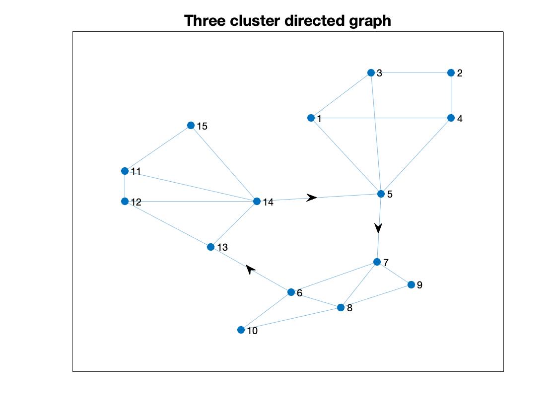
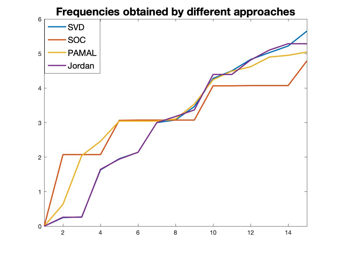
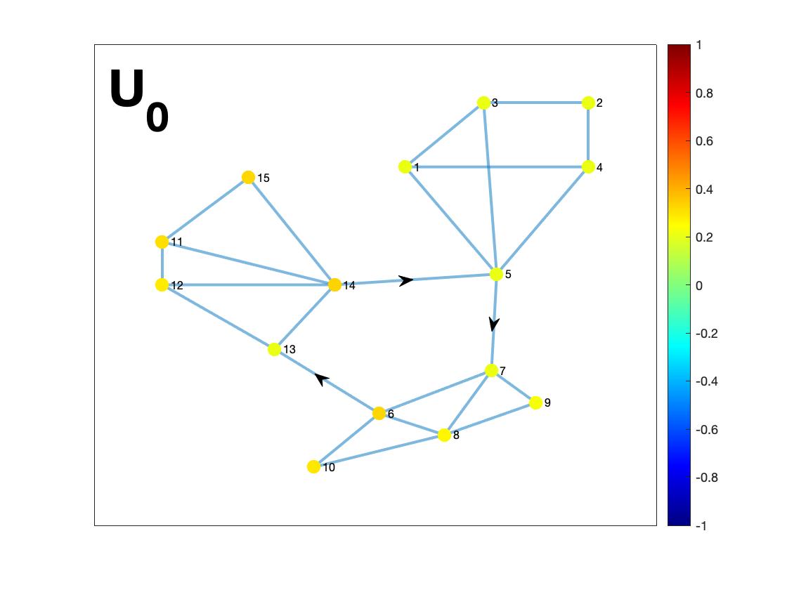
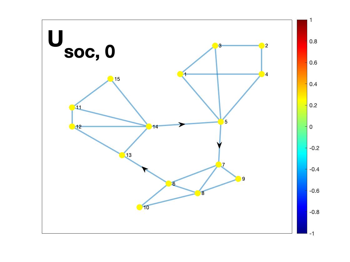
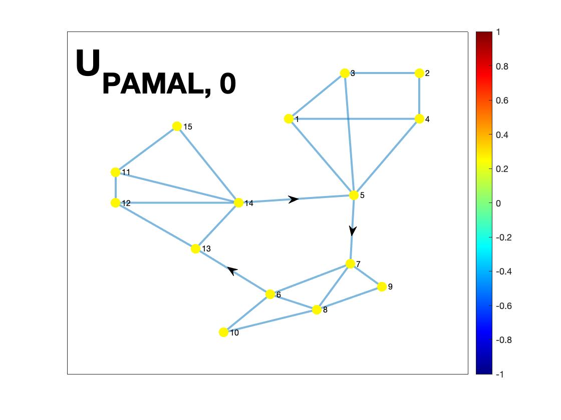
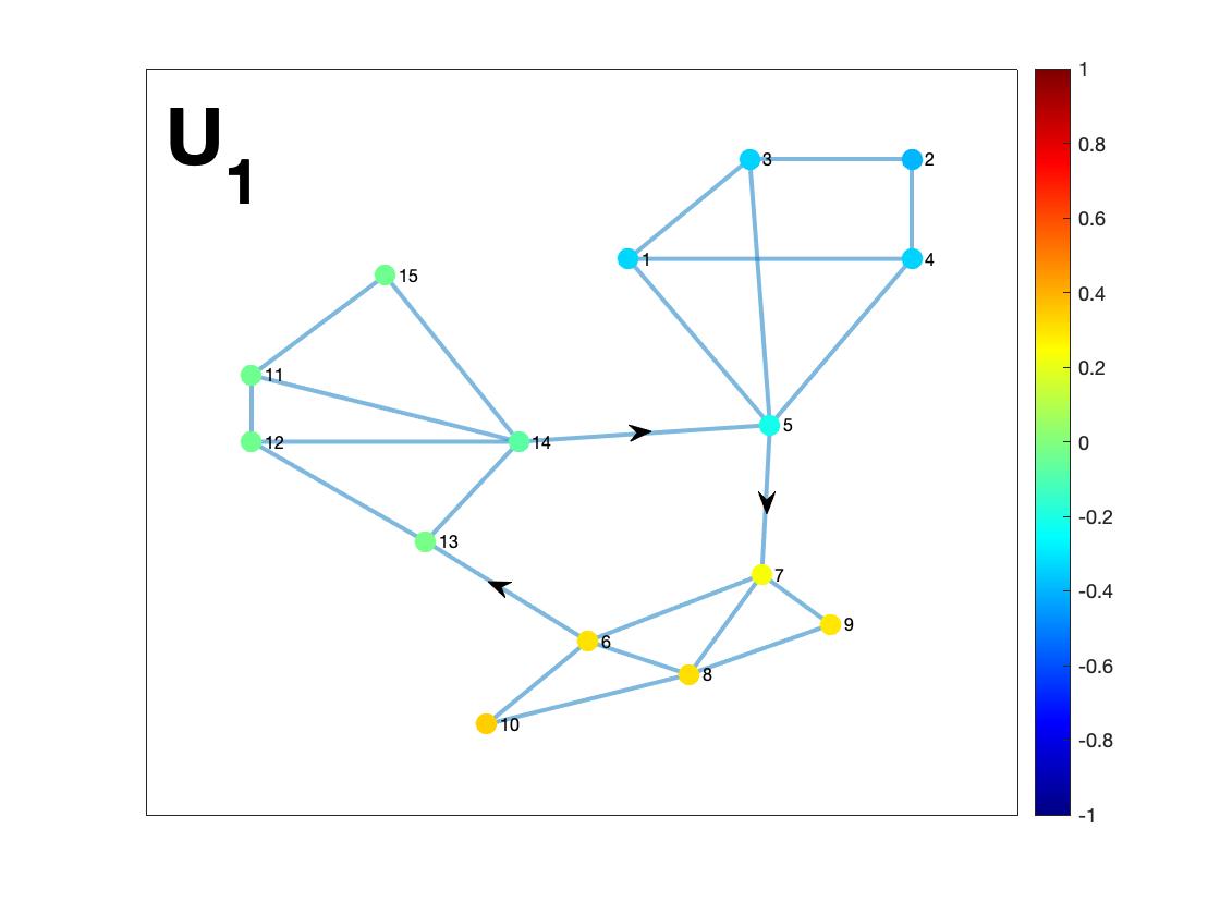
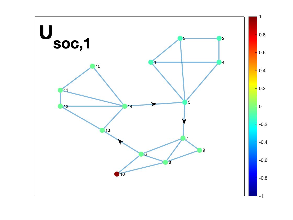
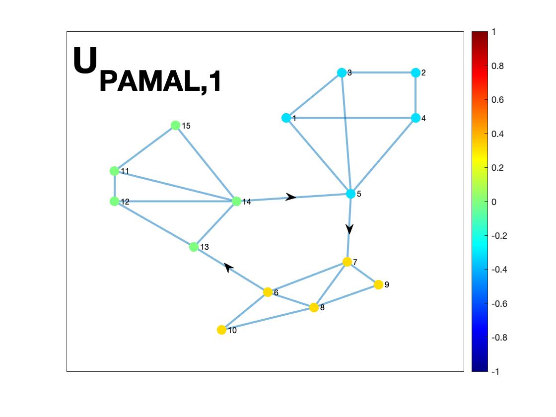
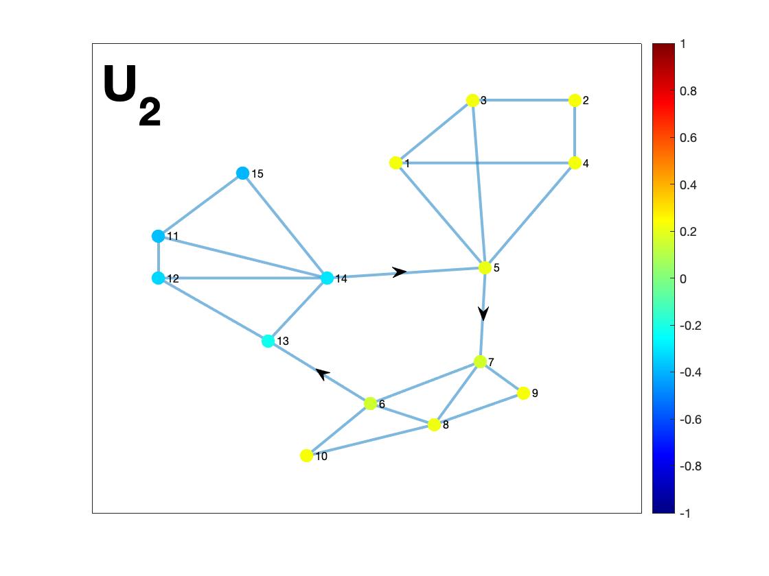
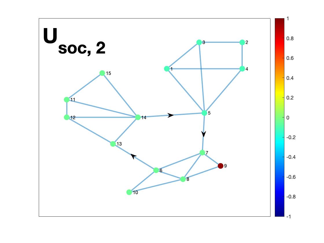
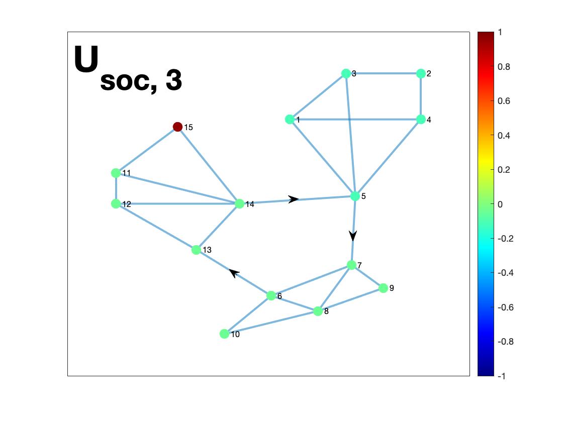
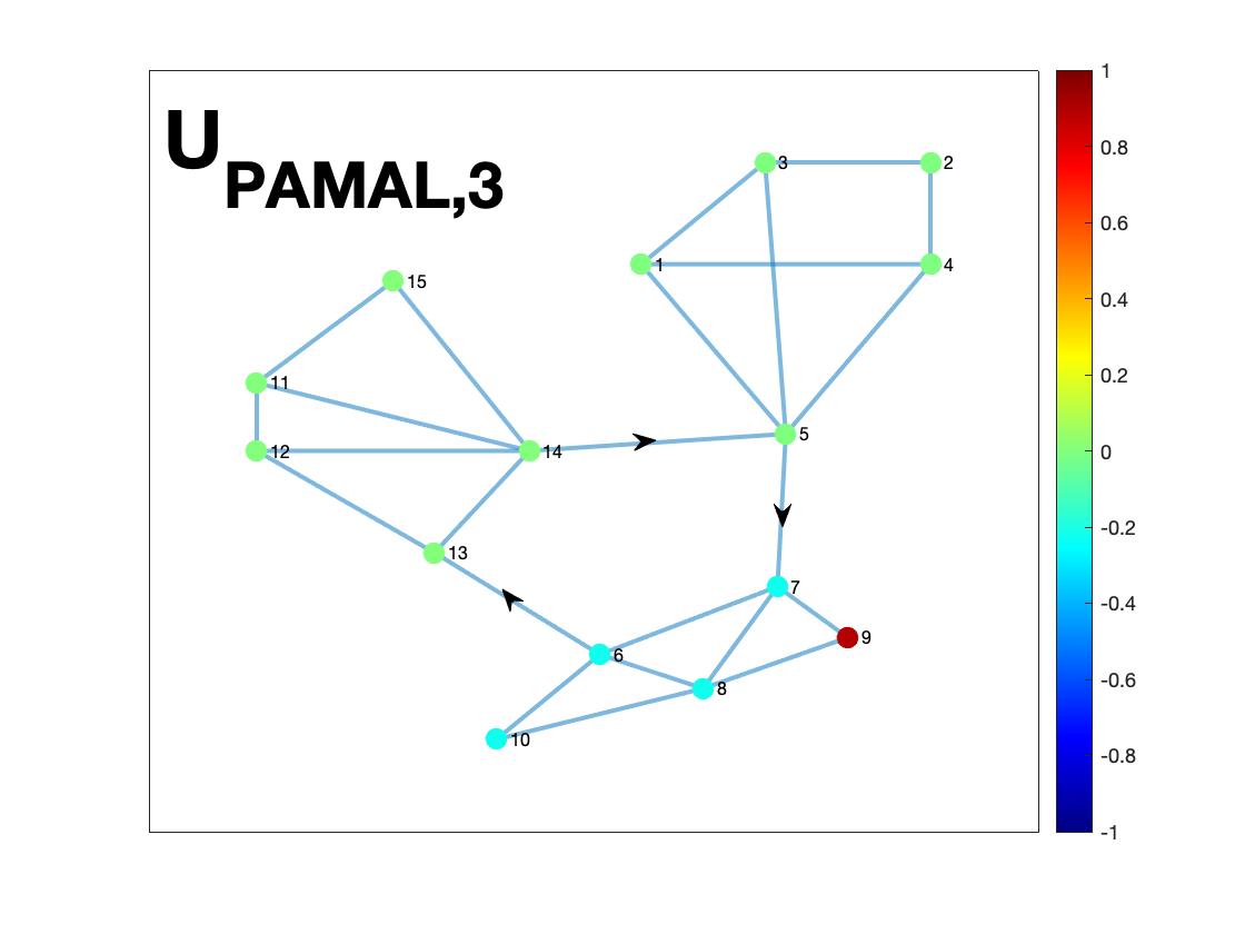
Figure 2: Plotted on the top left is a directed unweighted graph with three clusters of 5 knots connected with a directed cycle [13, Fig. 1(c)], and on the top right are its 15 frequencies via the SOC, PAMAL, Jordan and the proposed SVD approach. On the next four rows from left to right are left frequency components, right frequency components of our proposed GFT, the SOC and PAMAL frequency components associated with $i$-th frequency, where $i=0,1,2,3$ from top to bottom.

For $0\leq i\leq N-1$, we obtain from the SVD (I.4) that ${\bf u}_{i}$ and ${\bf v}_{i}$ in (I.5) are the left and right eigenvectors of ${\bf L}^{T}{\bf L}$ associated with the eigenvalue $\sigma_{i}^{2}$, i.e.,

$${\bf u}_{i}^{T}{\bf L}^{T}{\bf L}=\sigma_{i}^{2}{\bf u}_{i}^{T}\ \ {\rm and}\ \ {\bf L}^{T}{\bf L}{\bf v}_{i}=\sigma_{i}^{2}{\bf v}_{i},\ 0\leq i\leq N-1,$$ (III.4)

[21, 29]. Then we call ${\bf u}_{i}$ and ${\bf v}_{i},0\leq i\leq N-1$, as the left and right frequency components associated with frequency $\sigma_{i}$, or $i$-th left (right) frequency components in short, respectively. By (II.1), the right frequency component associated with frequency zero can be selected as follows,

$${\bf v}_{0}=N^{-1/2}{\bf 1}.$$ (III.5)

The left frequency component ${\bf u}_{0}$ associated with frequency zero is not always a multiple of the constant signal ${\bf 1}$. One may verify that it can be so chosen that

$${\bf u}_{0}=N^{-1/2}{\bf 1}$$ (III.6)

if and only if ${\mathcal{G}}$ is an Eulerian graph, in which the in-degree and out-degree are the same at each vertex.

In the undirected graph setting, the left and right frequency components can be selected as the same, and they can be obtained via solving a family of constrained optimization problems inductively,

$${\bf u}_{i}={\bf v}_{i} \hskip-5.78172pt= \hskip-5.78172pt\arg\min_{{\bf x}\in W_{i}^{\perp}\ {\rm with}\ \|{\bf x}\|_{2}=1}{\rm QV}({\bf x})$$ (III.7)

$$\hskip-5.78172pt= \hskip-5.78172pt\arg\min_{{\bf x}\in W_{i}^{\perp}\ {\rm with}\ \|{\bf x}\|_{2}=1}\|{\bf L}{\bf x}\|_{2},$$

with the initial ${\bf v}_{0}=N^{-1/2}\bf 1$, where quadratic variation ${\rm QV}({\bf x})$ of a graph signal ${\bf x}$ is given in (I.6), and for $1\leq i\leq N-1$, $W_{i}^{\perp}$ is the orthogonal complement of the space spanned by ${\bf v}_{j},0\leq j\leq i-1$. Denote the average and standard deviation of a vector ${\bf x}\in{\mathbb{R}}^{N}$ by

$$m({\bf x})=N^{-1}{\bf 1}^{T}{\bf x}\ \ {\rm and}\ \ {\rm SD}({\bf x})=N^{-1/2}\|{\bf x}-m({\bf x}){\bf 1}\|_{2},$$

the null space of the transpose of Laplacian ${\bf L}$ by ${\rm ker}({\bf L}^{T})$, and the dimension of a linear space $W$ by $\dim W$. Based on the standard algorithm to find SVD and Courant-Fischer-Weyl min-max principle, we can apply the following approach to construct frequencies $\sigma_{i}$ and frequency components ${\bf v}_{i}$ and ${\bf u}_{i},0\leq i\leq N-1$, of the proposed GFT:

$$\sigma_{0}=0\ \ {\rm and}\ \ {\bf v}_{0}=N^{-1/2}{\bf 1}$$ (III.8a)

for $$i=0$$, and

$$\left\{\begin{array}[]{rcl}\sigma_{i}&\hskip-5.78172pt=&\hskip-5.78172pt\min_{{\bf x}\in W_{i}^{\perp}\ {\rm with}\ \|{\bf x}\|_{2}=1}\|{\bf L}{\bf x}\|_{2}\\ &\hskip-5.78172pt=&\hskip-5.78172pt\min_{\dim W=i+1}\max_{{\bf x}\in W,\|{\bf x}\|_{2}=1}\|{\bf L}{\bf x}\|_{2}\\ &\hskip-5.78172pt=&\hskip-5.78172pt\max_{\dim W=N-i}\min_{{\bf x}\in W,\|{\bf x}\|_{2}=1}\|{\bf L}{\bf x}\|_{2}\\ {\bf v}_{i}&\hskip-5.78172pt=&\hskip-5.78172pt\arg\min_{{\bf x}\in W_{i}^{\perp}\ {\rm with}\ \|{\bf x}\|_{2}=1}\|{\bf L}{\bf x}\|_{2}\end{array}\right.$$ (III.8b)

inductively for $$1\leq i\leq N-1 {\bf u}_{i},0\leq i\leq i_{0} {\rm ker}({\bf L}^{T})$$, and let , be an orthonormal basis of the null space with

$${\bf u}_{0}={\rm arg}\min_{{\bf x}\in{\rm ker}({\bf L}^{T})\ {\rm with}\ \|{\bf x}\|_{2}=1\ {\rm and}\ m({\bf x})\geq 0}{\rm SD}({\bf x}),$$ (III.8c)

and define

$${\bf u}_{i}=\sigma_{i}^{-1}{\bf L}{\bf v}_{i},\ i_{0}<i\leq N-1,$$ (III.8d)

where $i_{0}$ is the largest index such that $\sigma_{i_{0}}=0$. We remark that the left frequency component ${\bf u}_{0}$ associated with zero frequency in the above construction satisfies (III.6) if ${\mathcal{G}}$ is an Eulerian graph, and that $i_{0}=0$ if the Laplacian ${\mathbf{L}}$ has rank $N-1$, or equivalently if the graph ${\mathcal{G}}$ is connected. Shown in Figure 2 are frequencies and frequency components of a directed unweighted graph of size $15$ containing three clusters connected by a directed cycle [13, Fig. 1(c)]. We observe that frequency components with low frequencies may have certain clustering property and oscillation pattern related to the graph topology.

In addition to the quadratic variation ${\rm QV}({\bf x})$ in (I.6) and $\|{\bf L}{\bf x}\|_{2}$ in (III.8), several directed variations have been proposed to measure the variation of a graph signal ${\bf x}=(x_{i})_{i\in V}$ along the directed graph structure, including

$${\rm GDV}({\bf x})=\sum_{i,j\in V}a_{ji}(x_{i}-x_{j})_{+}$$ (III.9)

and

$${\rm DV}({\bf x})=\sum_{i,j\in V}a_{ji}((x_{i}-x_{j})_{+})^{2}$$ (III.10)

where weight $a_{ij}$ is the $(i,j)$-th entry of the adjacent matrix ${\bf A}$ and $t_{+}=\max(t,0)$ for any real number $t\in{\mathbb{R}}$ [13, 16]. We finish this section with some comparisons among the GFT in Definition II.1 and the GFTs in [13, 16].

Remark III.1.

In [13], the authors use the directed variation ${\rm GDV}({\bf x})$ in (III.9) as Lovász extension of the cut size function, and define the GFT with frequency components ${\bf v}_{i}$ and frequencies $\lambda_{i}={\rm GDV}({\bf v}_{i}),0\leq i\leq N-1$, being ordered so that $\lambda_{0}\leq\lambda_{1}\leq\ldots\leq\lambda_{N-1}$, where ${\bf V}=[{\bf v}_{0},\ldots,{\bf v}_{N-1}]$ is the solution of the following constrained minimization problem

$$\min_{\bf V}\sum_{i=0}^{N-1}{\rm GDV}({\bf v}_{i})$$ (III.11)

subject to ${\bf V}^{T}{\bf V}={\bf I}$ and ${\bf v}_{0}=N^{-1/2}{\bf 1}$. To deal with the nonsmooth objective function and non-convex orthogonality constraints in (III.11), the authors present two iterative algorithms, splitting orthogonality constraints (SOC for abbreviation) and proximal alternating minimization augmented Lagrange (PAMAL for abbreviation), to solve relaxed versions of the constrained minimization problem (III.11), see [13, Algorithms 1, 2, 3]. The above two implementations are more numerically stable than the method (I.3) based on the Jordan decomposition of Laplacian, however they may fail to describe different modes of variation over the directed graph. Compared with the GFT proposed in this paper where only the SVD of the Laplacian matrix of size $N\times N$ is required, it needs to perform SVD of a matrix of size $N\times N$ at each iteration step of the iterative SOC and PAMAL algorithms.

In [16], the authors use the directed variation ${\rm DV}({\bf x})$ in (III.10) to measure the signal variation along the graph structure, and define the GFT with frequency components ${\bf v}_{i}$ and frequencies $\lambda_{i}={\rm DV}({\bf v}_{i}),0\leq i\leq N-1$, being ordered so that $\lambda_{0}\leq\lambda_{1}\leq\ldots\leq\lambda_{N-1}$, where ${\bf V}=[{\bf v}_{0},\ldots,{\bf v}_{N-1}]$ is the solution of the following constrained problem,

$$\min_{\bf V}\sum_{i=1}^{N-1}|{\rm DV}({\bf v}_{i})-{\rm DV}({\bf v}_{i-1})|^{2}$$ (III.12)

subject to ${\bf V}^{T}{\bf V}={\bf I}$, ${\bf v}_{0}=N^{-1/2}{\bf 1}$ and ${\bf v}_{N-1}=\arg\max_{\|{\bf v}\|_{2}=1}{\rm DV}({\bf v})$. Based on the feasible method for optimization over the Stiefel manifold in [30], the authors develop an iterative algorithm to solve the constrained problem (III.12), see [16, Algorithms 1 and 2]. At each iteration, the proposed algorithm involves a matrix inversion and the computational complexity is about $O(N^{3})$. Also as mentioned in [16, Remark 1], for the directed cycle graph (the circulant graph ${\mathcal{C}}_{d}(N,Q)$ generated by $Q=\{1\}$), the proposed GFT in [16] fails to obtain the discrete Fourier transform in (II.19), cf. Theorem II.2 for our SVD-based GFT in the directed circulant graph setting.

IV Graph Fourier transform on directed Eulerian graphs

Let ${\mathcal{E}}=(V,E)$ be an Eulerian graph of order $N$ containing no loops or multiple edges, and ${\mathcal{E}}_{t},0\leq t\leq 1$, be a family of directed Eulerian graphs that share the same vertex set $V$ with the graph ${\mathcal{E}}$ and have adjacent matrices ${\bf A}_{t}=(1-t){\bf A}+t{\bf A}^{T}$ being linear combinations of the adjacent matrices of the graph ${\mathcal{E}}$ and its transpose graph ${\mathcal{E}}^{T}$. In this section, we consider frequencies, frequency components and graph Fourier transforms on Eulerian graphs ${\mathcal{E}}_{t},0\leq t\leq 1$, to connect the graph ${\mathcal{E}}$ and its transpose graph ${\mathcal{E}}^{T}$. It is observed that frequencies and frequency components on the Eulerian graphs ${\mathcal{E}}_{t},0\leq t\leq 1$, have certain symmetric properties, see (IV.9) and Theorem IV.2. We say that frequencies $\sigma_{i}(t),0\leq i\leq N-1$, of the Eulerian graphs ${\mathcal{E}}_{t},0\leq t\leq 1$, are simple if

$$0=\sigma_{0}(t)<\sigma_{1}(t)<\ldots<\sigma_{N-1}(t),\ 0\leq t\leq 1.$$ (IV.1)

In Theorem IV.1, we show that frequencies and frequency components are differentiable about $0\leq t\leq 1$, if frequencies of the Eulerian graphs ${\mathcal{E}}_{t},0\leq t\leq 1$, are simple. To quantify and measure the degree of asymmetry of the Eulerian graph ${\mathcal{E}}$, we define

$$\sigma_{\rm asym}=\max_{\|{\bf x}\|_{2}=1}\|({\mathbf{L}}-{\bf L}^{T}){\bf x}\|_{2},$$ (IV.2)

which is the same as the largest singular value of ${\mathbf{L}}-{\bf L}^{T}$ [31]. From the estimation in Theorem IV.1, we conclude that frequencies and frequency components have slow variations to $0\leq t\leq 1$ when $\sigma_{\rm asym}$ is small, see (IV.16) and (IV.17).

Recall that an Eulerian graph ${\cal E}$ has the same in-degree and out-degree at each vertex, the Laplacians ${\bf L}_{t}$ of the graphs ${\mathcal{E}}_{t}$ are given by

$${\mathbf{L}}_{t}=(1-t){\bf L}+t{\bf L}^{T},$$ (IV.3)

and satisfy

$${\mathbf{L}}_{t}{\bf 1}={\bf 0},\ 0\leq t\leq 1.$$ (IV.4)

By the continuity of the Laplacian ${\mathbf{L}}_{t},0\leq t\leq 1$, we can find an SVD

$${\bf L}_{t}={\bf U}_{t}{\boldsymbol{\Sigma}}_{t}{\bf V}_{t}^{T}$$ (IV.5)

with initials $({\bf U}_{0},{\bf V}_{0},{\boldsymbol{\Sigma}}_{0})=({\bf U},{\bf V},{\boldsymbol{\Sigma}})$ such that orthogonal matrices ${\bf U}_{t},{\bf V}_{t}$ and diagonal matrices

$${\boldsymbol{\Sigma}}_{t}={\rm diag}(\sigma_{0}(t),\ldots,\sigma_{N-1}(t))$$ (IV.6)

of singular values of Laplacians ${\mathbf{L}}_{t}$ in a nondecreasing order are continuous about $0\leq t\leq 1$, where ${\mathbf{L}}={\bf U}{\boldsymbol{\Sigma}}{\bf V}^{T}$ is the SVD (I.4) of the Laplacian ${\mathbf{L}}$. Using the above SVD of ${\mathbf{L}}_{t}$, we can define GFT ${\mathcal{F}}_{t}$ of a signal ${\bf x}$ on the graph ${\mathcal{E}}_{t}$ (and also on ${\mathcal{E}}={\mathcal{E}}_{0}$ as they have the same vertex set) by

$${\mathcal{F}}_{t}{\bf x}=\frac{1}{2}\begin{pmatrix}{\bf U}_{t}^{T}{\bf x}+{\bf V}_{t}^{T}{\bf x}\\ {\bf U}_{t}^{T}{\bf x}-{\bf V}_{t}^{T}{\bf x}\end{pmatrix},\ 0\leq t\leq 1.$$ (IV.7)

By (IV.4), we have

$$\sigma_{0}(t)=0,\ 0\leq t\leq 1.$$ (IV.8)

By the SVD (IV.5), $(\sigma_{i}(t))^{2},0\leq i\leq N-1$, are eigenvalues of matrices ${\mathbf{L}}_{t}^{T}{\mathbf{L}}_{t}$ and ${\mathbf{L}}_{t}{\mathbf{L}}_{t}^{T}$. This together with the nonnegative nondecreasing order of singular values $\sigma_{i}(t),0\leq i\leq N-1$, and the observation that ${\mathbf{L}}_{1-t}{\mathbf{L}}_{1-t}^{T}={\mathbf{L}}_{t}^{T}{\mathbf{L}}_{t},\ 0\leq t\leq 1$, proves that

$$\sigma_{i}(1-t)=\sigma_{i}(t),\ 0\leq t\leq 1.$$ (IV.9)

Shown in Figure 3 are the graph frequencies $\sigma_{i}(t),0\leq i\leq N-1$, of Eulerian graphs ${\mathcal{E}}_{t},0\leq t\leq 1$ of order $N=64$.

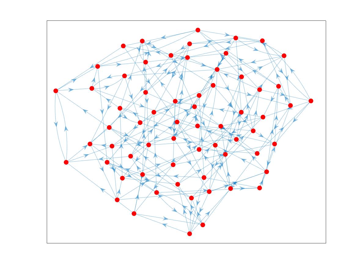
Figure 3: Plotted on the left is an Eulerian graph of order $N=64$ with the associated Laplacian ${\bf L}$ being a double stochastic matrix with $\sigma_{\rm asym}=20.2248$. On the right is the frequencies $\sigma_{i}(t),0\leq i\leq N-1$, of graph Laplacian matrices ${\bf L}_{t}=(1-t){\bf L}+t{\bf L}^{T}$ with their maximal variation $\max_{0\leq i\leq N-1}\max_{0\leq t\leq 1}|\sigma_{i}(t)-\sigma_{i}(1/2)|=1.6750$.

Observe from (IV.3) that ${\mathbf{L}}_{t},0\leq t\leq 1$, satisfy

$${\mathbf{L}}_{t}-{\mathbf{L}}_{s}=(t-s)({\mathbf{L}}^{T}-{\mathbf{L}}),\ 0\leq t,s\leq 1.$$ (IV.10)

This together with the Courant-Fischer-Weyl min-max principle,

$$\sigma_{i}(t) \hskip-5.78172pt= \hskip-5.78172pt\min_{\dim W=i+1}\max_{{\bf x}\in W,\|{\bf x}\|_{2}=1}\|{\bf L}_{t}{\bf x}\|_{2}$$

$$\hskip-5.78172pt= \hskip-5.78172pt\max_{\dim W=N-i}\min_{{\bf x}\in W,\|{\bf x}\|_{2}=1}\|{\bf L}_{t}{\bf x}\|_{2}$$

implies that $\sigma_{i}(t),0\leq i\leq N-1$, are Lipschitz functions,

$$|\sigma_{i}(t)-\sigma_{i}(s)|\leq\sigma_{\rm asym}|t-s|,\ 0\leq t,s\leq 1.$$ (IV.11)

In the following theorem, we consider the differentiability of frequencies and left/right frequency components with respect to $0\leq t\leq 1$, when $\sigma_{i}(t),0\leq i\leq N-1$, are simple. By (IV.11), we see that the simple requirement (IV.1) is met if all eigenvalues of Laplacian on ${\mathcal{E}}_{1/2}$ are simple, and the directed Eulerian graph ${\mathcal{E}}$ is close to its undirected counterpart ${\mathcal{E}}_{1/2}$ in the sense that

$$0<\sigma_{\rm asym}\leq\alpha\min_{1\leq i\leq N-1}\sigma_{i}(1/2)-\sigma_{i-1}(1/2)$$

for some $0<\alpha<1$.

Theorem IV.1.

Let ${\mathcal{E}}_{t},0\leq t\leq 1$, be the family of directed Eulerian graphs to connect a directed Eulerian graph ${\mathcal{E}}$ and its transpose graph ${\mathcal{E}}^{T}$, and the associated Laplacian ${\bf L}_{t}$ in (IV.3) has the SVD (IV.5) with orthogonal matrices ${\bf U}_{t}=[{\bf u}_{0}(t),\ldots,{\bf u}_{N-1}(t)]$ and ${\bf V}_{t}=[{\bf v}_{0}(t),\ldots,{\bf v}_{N-1}(t)],\ 0\leq t\leq 1$ being continuous about $0\leq t\leq 1$ and satisfying

$${\bf u}_{0}(t)={\bf v}_{0}(t)=N^{-1/2}{\bf 1}.$$ (IV.12)

Then for any $1\leq i\leq N-1$, the $i$-th frequency and frequency components of the graph Fourier transform ${\mathcal{F}}_{t},0\leq t\leq 1$ is differentiable about $t$ if it is a simple singular value, i.e., $\sigma_{i}(t)\neq\sigma_{j}(t)$ for all $j\neq i$. Moreover, for all $1\leq i\leq N-1$,

$$\frac{d\sigma_{i}(t)}{dt}=({\bf v}_{i}(t))^{T}({\bf L}^{T}-{\bf L}){\bf u}_{i}(t),$$ (IV.13)

$$\frac{d{\bf u}_{i}(t)}{dt}=\sum_{k=1}^{N-1}\Big{(}-b_{i,k}(t)({\bf v}_{k}(t))^{T}({\bf L}^{T}-{\bf L}){\bf u}_{i}(t)+a_{i,k}(t)({\bf u}_{k}(t))^{T}({\bf L}^{T}-{\bf L}){\bf v}_{i}(t)\Big{)}{\bf u}_{k}\quad$$ (IV.14)

and

$$\frac{d{\bf v}_{i}(t)}{dt}=\sum_{k=1}^{N-1}\Big{(}-a_{i,k}(t)({\bf v}_{k}(t))^{T}({\bf L}^{T}-{\bf L}){\bf u}_{i}(t)+b_{i,k}(t)({\bf u}_{k}(t))^{T}({\bf L}^{T}-{\bf L}){\bf v}_{i}(t)\Big{)}{\bf v}_{k},\quad$$ (IV.15)

where

$$a_{i,k}(t)=\left\{\begin{array}[]{ll}\sigma_{i}(t)((\sigma_{i}(t))^{2}-(\sigma_{k}(t))^{2})^{-1}&{\rm if}\ k\neq i\\ (4\sigma_{i}(t))^{-1}&{\rm if}\ k=i,\end{array}\right.$$

and

$$b_{i,k}(t)=\left\{\begin{array}[]{ll}\sigma_{k}(t)((\sigma_{i}(t))^{2}-(\sigma_{k}(t))^{2})^{-1}&{\rm if}\ k\neq i\\ (-4\sigma_{i}(t))^{-1}&{\rm if}\ k=i.\end{array}\right.$$

The detailed proof of Theorem IV.1 will be given in Appendix -B. By Theorem IV.1, we have

$$\left|\frac{d\sigma_{i}(t)}{dt}\right|\leq\sigma_{\rm asym}.$$ (IV.16)

Set

$$C(t)=\max_{1\leq i,k\leq N-1}|a_{i,k}(t)|+\max_{1\leq i,k\leq N-1}|b_{i,k}(t)|.$$

The orthogonality of the matrices $\bf U$ and $\bf V$ implies that

$$\left\|\frac{d{\bf u}_{i}(t)}{dt}\right\|_{2}\hskip-3.61371pt \leq\hskip-3.61371pt \hskip-3.61371pt\max_{1\leq i,k\leq N-1}|a_{i,k}(t)|\ \|({\bf L}^{T}-{\bf L}){\bf u}_{i}(t)\|_{2}+\max_{1\leq i,k\leq N-1}|b_{i,k}(t)|\ \|({\bf L}^{T}-{\bf L}){\bf v}_{i}(t)\|_{2}\leq C(t)\sigma_{\rm asym}.$$

Following a similar argument to $\left\|\frac{d{\bf v}_{i}(t)}{dt}\right\|_{2}$, we have

$$\max\left(\left\|\frac{d{\bf u}_{i}(t)}{dt}\right\|_{2},\left\|\frac{d{\bf v}_{i}(t)}{dt}\right\|_{2}\right)\leq C(t)\sigma_{\rm asym}.$$ (IV.17)

This concludes that frequencies and frequency components have small variation about $0\leq t\leq 1$ when the degree $\sigma_{\rm asym}$ of asymmetry of the Eulerian graph ${\mathcal{E}}$ is small.

Under the simplicity assumption (IV.1) for all singular values $\sigma_{i}(t),0\leq i\leq N-1$, in addition to the symmetry (IV.9) for the graph frequencies, we have the certain symmetric property for the orthogonal matrices ${\bf U}_{t}$ and ${\bf V}_{t},0\leq t\leq 1$, see Appendix -C for the detailed proof.

Theorem IV.2.

Let the family of directed Eulerian graph ${\mathcal{E}}_{t},0\leq t\leq 1$, the associated Laplacian ${\bf L}_{t}$, the singular value decomposition ${\bf L}_{t}={\bf U}_{t}{\boldsymbol{\Sigma}}_{t}{\bf V}_{t}$ be as in Theorem IV.1. If the singular values $\sigma_{i}(t),0\leq i\leq N-1$, satisfy (IV.1), then for all $0\leq t\leq 1$,

$${\bf U}_{t}={\bf V}_{1-t},$$ (IV.18)

and

$${\mathcal{F}}_{1-t}{\bf x}=\begin{pmatrix}{\bf I}&{\bf 0}\\ {\bf 0}&-{\bf I}\end{pmatrix}{\mathcal{F}}_{t}{\bf x}$$ (IV.19)

where ${\bf x}$ is a graph signal on the Eulerian graph ${\mathcal{E}}$.

For the case that ${\mathcal{E}}$ is an undirected graph (hence an Eulerian graph), the orthogonal matrices ${\bf U}_{t}$ and ${\bf V}_{t},0\leq t\leq 1$, in the singular value decomposition (IV.5) can be chosen to be independent on $t$. The converse is true as well, because ${\bf U}_{t}={\bf U}_{1/2}={\bf V}_{1/2}={\bf V}_{t},0\leq t\leq 1$, by the independence of orthogonal matrices ${\bf U}_{t}$ and ${\bf V}_{t}$ on $0\leq t\leq 1$ and the observation that the Eulerian graph ${\mathcal{G}}_{1/2}$ is undirected, we have that ${\bf L}^{T}={\bf L}$ and ${\mathcal{E}}$ is undirected. In the following theorem, we show that $({\bf L}^{T})^{2}={\mathbf{L}}^{2}$ is a necessary condition for any pair of orthogonal matrices ${\bf U}_{t}$ and ${\bf V}_{t},0\leq t\leq 1$, are identical, see Appendix -D for the proof.

Theorem IV.3.

Let ${\bf U}_{t},{\bf V}_{t}$ be the orthogonal matrices in the singular value decomposition (IV.5) of the Laplacian ${\mathbf{L}}_{t}$ in (IV.3). If there exists $t_{0}\neq t_{1}\in[0,1]$ such that

$${\bf U}_{t_{0}}={\bf U}_{t_{1}}\ {\rm and}\ {\bf V}_{t_{0}}={\bf V}_{t_{1}},$$ (IV.20)

then $({\bf L}^{T})^{2}={\mathbf{L}}^{2}$.

V Numerical simulations

Graph Fourier transform should be designed to decompose graph signals into different frequency components, to represent them by different modes of variation efficiently, and to have energy of smooth graph signals concentrated mainly at low frequencies. In this section, we demonstrate the performance of the proposed SVD-based GFT to denoise the hourly temperature data set collected at 218 locations in the United States on August 1st, 2010 via the bandlimiting ${\bf P}_{M}$ at the first $M$-frequencies [28, 33, 34]. Here for the SVD-based GFT proposed in this paper, the bandlimiting ${\bf P}_{M}$ of a graph signal ${\bf x}$ at the first $M$-frequencies is given by

$${\bf P}_{M}{\bf x}=\!{\mathcal{F}}^{-1}\begin{pmatrix}{\bf\chi}_{M}&\!{\bf O}\\ {\bf O}&\!{\bf\chi}_{M}\end{pmatrix}{\mathcal{F}}{\bf x}\!=\frac{1}{2}\!\sum_{i=0}^{M-1}\langle{\bf x},{\bf u}_{i}\rangle{\bf u}_{i}+\langle{\bf x},{\bf v}_{i}\rangle{\bf v}_{i},$$

where $\chi_{M}$ is a diagonal matrix with the first $M$ diagonal entries taking value one and all others taking value zero, and for $0\leq i\leq M-1$, the $i$-th left/right frequency components ${\bf u}_{i},{\bf v}_{i}$ are $i$-th columns of orthogonal matrices ${\bf U}$ and ${\bf V}$ in the SVD (I.4) respectively. For the GFT defined by splitting orthogonality constraints (SOC) and proximal alternating minimized augmented Lagrangian (PAMAL), the bandlimiting ${\bf P}_{M}$ of a graph signal ${\bf x}$ at the first $M$-frequencies is given by

$${\bf P}_{M}{\bf x}=\sum_{i=0}^{M-1}\langle{\bf x},{\bf v}_{i}\rangle{\bf v}_{i}$$

where ${\bf v}_{i},0\leq i\leq M-1$, is the $i$-th frequency component in [13].

Let the underlying graph $\cal G$ of the US weather data set have $218$ vertices representing locations of weather stations, edges given by 5-nearest neighboring stations in physical distances, and weights on the edges are randomly chosen in $[0.8,1.2]$, and denote the US temperature measured in Fahrenheit on August 1st, 2010 by ${\bf x}(t_{k}),1\leq k\leq 24$, see [34, Fig. 6] for two snapshots of the data set. Shown in Figure 4 are the denoising performances in ISNR and SNR to apply the bandlimiting projection ${\bf P}_{M}$ to the noisy observations

$${\bf y}(t_{k})={\bf x}(t_{k})+{\boldsymbol{\eta}}(t_{k}),1\leq k\leq 24,$$ (V.1)

corrupted with additive random noises ${\boldsymbol{\eta}}(t_{k})$ with entries being i.i.d. and having mean zero and variance $c\in[4,16]$. Here the input signal-to-noise ratio (ISNR) and the output signal-to-noise ratio (SNR) are defined by

$${\rm ISNR}=-20\log_{10}\frac{\|{\boldsymbol{\eta}}\|_{2}}{\|{\bf x}\|_{2}}\ {\rm and}\ {\rm SNR}=-20\log_{10}\frac{\|\widehat{\bf x}-{\bf x}\|_{2}}{\|{\bf x}\|_{2}},$$

where the original signal ${\bf x}$, the noisy measurement ${\bf y}$ and the denoised signal $\widehat{\bf x}$ are given by the hourly weather data ${\bf x}(t_{k})$, the noisy weather data ${\bf y}(t_{k})$ in (V.1), and the denoised signal ${\bf P}_{M}{\bf y}(t_{k})$ by bandlimiting ${\bf P}_{M}$ the noisy weather data ${\bf y}(t_{k})$ to the first $M$-frequencies respectively. We observe from Figure 4 that the SVD-based GFT proposed in this paper outperforms the SOC and PAMAL-based GFTs in [13] on denoising the US hourly weather data set on August 1st, 2010 by bandlimiting ${\bf P}_{M}$ at the first $M$-frequencies. It is also noticed that the SOC and PAMAL-based GFTs in [13] have very similar performance on denoising the weather data set. The possible reason is that they are based on different relaxations of the same constrained minimization problem (III.11).

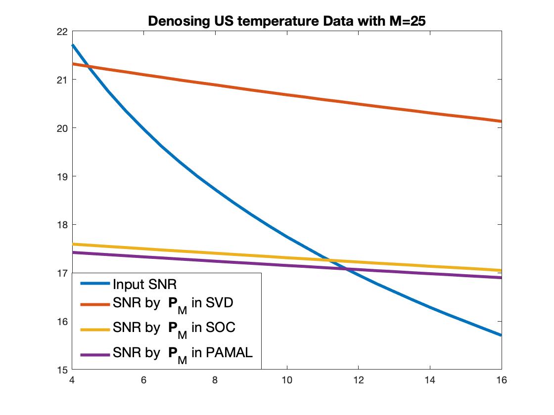
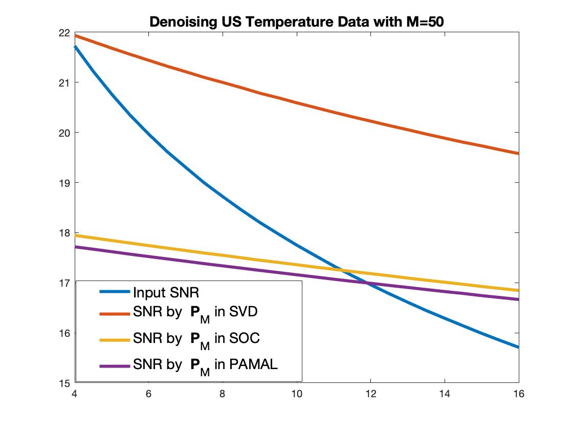
Figure 4: Plotted are the averages of ISNR and SNR of denoising the hourly temperature data ${\bf y}(t_{k}),1\leq k\leq 24$, on August 1st, 2012 over $1000\times 24$ trials, via bandlimiting ${\bf P}_{M}$ at the first $M$-frequencies of the SVD, SOC and PAMAL-based GFTs, where $M=25$ (left) and $M=50$ (right).

In the appendix, we collect the proofs of Theorems II.2, IV.2 and IV.3.

-A Graph Fourier transform on circulant graphs

In this appendix, we consider GFT on circulant graphs and provide a proof of Theorem II.2.

Write $Q=\{q_{1},\ldots,q_{L}\}$ with $1\leq q_{1}<q_{2}<\ldots<q_{L}\leq N-1$, and ${\bf W}=[{\bf w}_{0},\ldots{\bf w}_{N-1}]$. Observe that the Laplacian matrix ${\mathbf{L}}_{{\mathcal{C}}_{d}}=(c_{ij})_{0\leq i,j\leq N-1}$ on the circulant graph ${\mathcal{C}}_{d}:={\mathcal{C}}_{d}(N,Q)$ is a circulant matrix with $ij$-th entries $c_{ij},0\leq i,j\leq N-1$, given by

$$c_{ij}=\left\{\begin{array}[]{ll}L&{\rm if}\ j=i\\ -1&{\rm if}\ j-i\in Q\ {\rm mod}\ N\\ 0&{\rm otherwise}.\end{array}\right.$$

Then one may verify that

$${\mathbf{L}}_{{\mathcal{C}}_{d}}{\bf w}_{i}=P(\omega_{N}^{i}){\bf w}_{i},\ 0\leq i\leq N-1,$$ (.2)

where $P$ is the polynomial symbol of the circulant matrix ${\mathbf{L}}_{{\mathcal{C}}_{d}}$ defined by (II.11).

Let

$${\bf M}={\rm diag}(|P(1)|,|P(\omega_{N})|,\ldots,|P(\omega_{N}^{N-1})|)$$ (.3)

be the diagonal matrix with magnitudes $|P(\omega_{N}^{i})|,0\leq i\leq N-1$, of the symbol $P$ on all $N$-th unit roots. Then we can reformulate (.2) in the following matrix form,

$${\mathbf{L}}_{{\mathcal{C}}_{d}}{\bf W}={\bf W}{\boldsymbol{\Theta}}{\bf M},$$ (.4)

where ${\boldsymbol{\Theta}}$ is the diagonal matrix in (II.15).

Let ${\bf Q}$ be a permutation matrix to rearrange $|P(\omega_{N}^{i})|,0\leq i\leq N-1$, in nondecreasing order, with $0$ as the first index, and indices $i$ and $N-i,1\leq i<N/2$, next each other. This together with $|P(\omega_{N}^{i})|=|P(\omega_{N}^{N-i})|,1\leq i\leq N-1$, implies that the diagonal matrix ${\boldsymbol{\Sigma}}$ in (II.18) satisfies

$${\boldsymbol{\Sigma}}={\bf Q}{\bf M}{\bf Q}.$$ (.5)

Let ${\bf e}_{k},0\leq k\leq N-1$, be the unit vectors with zero entries except the $k$-th entry taking value $1$, and define the permutation matrices ${\bf P}_{0}$ and ${\bf P}_{1}$ by

$${\bf P}_{0}=\left\{\begin{array}[]{l}\!\big{[}{\bf e}_{0},{\bf e}_{1},{\bf e}_{N-1},\ldots,{\bf e}_{(N-1)/2},{\bf e}_{(N+1)/2}\big{]}\qquad\hfill{\rm if}\ N\ {\rm is\ odd}\\ \!\big{[}{\bf e}_{0},{\bf e}_{1},{\bf e}_{N-1},\ldots,{\bf e}_{N/2-1},{\bf e}_{N/2+1},{\bf e}_{N/2}\big{]}\qquad\hfill{\rm if}\ N\ {\rm is\ even}\end{array}\right.$$ (.6)

and

$${\bf P}_{1}={\bf P}_{0}{\bf Q}.$$ (.7)

Therefore the conclusion in Theorem II.2 about the GFT on the circulant graph ${\mathcal{C}}_{d}(N,Q)$ reduces to the singular value decomposition of ${\mathbf{L}}_{{\mathcal{C}}_{d}}$ in the following proposition.

Proposition .1.

Let ${\mathbf{L}}_{{\mathcal{C}}_{d}}$ be the Laplacian matrix on the circulant graph ${\mathcal{C}}_{d}:={\mathcal{C}}_{d}(N,Q)$, and ${\bf W},{\bf R},{\boldsymbol{\Theta}},{\boldsymbol{\Sigma}},{\bf P}_{0}$ and ${\bf P}_{1}$ be as in (II.12), (II.14), (II.15), (II.18), (.6) and (.7) respectively. Then the matrices ${\bf U}$ and ${\bf V}$ in (II.17) are orthogonal matrices with real entries, and the singular value decomposition (II.16) holds for the Laplacian matrix ${\mathbf{L}}_{{\mathcal{C}}_{d}}$.

Proof.

The conclusions are trivial for $N=1$ and $N=2$. So we assume that $N\geq 3$ now. First we divide two cases, $N\geq 3$ is odd and even, to prove that matrices ${\bf U}$ and ${\bf V}$ in (II.17) are orthogonal matrices with real entries. Define

$$\widetilde{\bf U}={\bf W}{\boldsymbol{\Theta}}{\bf P}_{0}{\bf R}=[\widetilde{\bf u}_{0},\widetilde{\bf u}_{1},\ldots,\widetilde{\bf u}_{N-1}]$$ (.8)

and

$$\widetilde{\bf V}={\bf W}{\bf P}_{0}{\bf R}=[\widetilde{\bf v}_{0},\widetilde{\bf v}_{1},\ldots,\widetilde{\bf v}_{N-1}].$$ (.9)

As ${\bf P}_{1}$ is a permutation matrix, ${\bf U}=\widetilde{\bf U}{\bf P}_{1}$ and ${\bf V}=\widetilde{\bf V}{\bf P}_{1}$, it suffices to show that $\widetilde{\bf U}$ and $\widetilde{\bf V}$ are orthogonal matrices with real entries.

Case 1:  $N=2K+1$ for some integer $K\geq 1$.

By (II.14), (.8) and (.9), we have

$$\widetilde{\bf u}_{0}=\widetilde{\bf v}_{0}={\bf w}_{0}=N^{-1/2}{\bf 1}\in{\mathbb{R}}^{N},$$ (.10)

and for $1\leq k\leq K$

$$\left\{\begin{array}[]{l}\widetilde{\bf v}_{2k-1}=\frac{{\bf w}_{k}+{\bf w}_{N-k}}{\sqrt{2}}=\frac{{\bf w}_{k}+\overline{\bf w}_{k}}{\sqrt{2}}\in{\mathbb{R}}^{N}\\ \widetilde{\bf v}_{2k}=\frac{{\bf w}_{k}-{\bf w}_{N-k}}{\sqrt{-2}}=\frac{{\bf w}_{k}-\overline{\bf w}_{k}}{\sqrt{-2}}\in{\mathbb{R}}^{N},\end{array}\right.$$ (.11)

and

$$\left\{\begin{array}[]{l}\widetilde{\bf u}_{2k-1}=\frac{\exp(\sqrt{-1}\theta_{k}){\bf w}_{k}+\exp(-\sqrt{-1}\theta_{k})\overline{{\bf w}_{k}}}{\sqrt{2}}\in{\mathbb{R}}^{N}\\ \widetilde{\bf u}_{2k}=\frac{\exp(\sqrt{-1}\theta_{k}){\bf w}_{k}-\exp(-\sqrt{-1}\theta_{k})\overline{{\bf w}_{k}}}{\sqrt{-2}}\in{\mathbb{R}}^{N}.\end{array}\right.$$ (.12)

Therefore $\widetilde{\bf U}$ and $\widetilde{\bf V}$ are square matrices with real entries. This together with the unitary property for the discrete Fourier transform matrix ${\bf W}$, the phase matrix ${\boldsymbol{\Theta}}$ and the rotation matrix ${\bf R}$, and the orthogonality of the permutation matrix ${\bf P}_{1}$ implies that

$${\widetilde{\bf U}}^{T}{\widetilde{\bf U}}=\widetilde{\bf U}^{H}\widetilde{\bf U}={\bf R}^{H}{\bf P}_{0}^{T}{\boldsymbol{\Theta}}^{H}{\bf W}^{H}{\bf W}{\boldsymbol{\Theta}}{\bf P}_{0}{\bf R}={\bf I}$$

and

$$\widetilde{\bf V}^{T}\widetilde{\bf V}=\widetilde{\bf V}^{H}\widetilde{\bf V}={\bf R}^{H}{\bf P}_{0}^{T}{\bf W}^{H}{\bf W}{\bf P}_{0}{\bf R}={\bf I}.$$

This proves that $\tilde{\bf U}$ and $\widetilde{\bf V}$ (and hence ${\bf U}$ and ${\bf V}$ in (II.17)) are orthogonal matrices with real entries for the case that $N$ is odd.

Case 2:  $N=2K+2$ for some integer $K\geq 1$.

Using the similar argument used in Case 1, we can show that (.10), (.11) and (.12) hold. In addition, we have

$$\widetilde{u}_{2K+1}=\widetilde{\bf v}_{2K+1}=N^{-1/2}(1,-1,\ldots,1,-1)^{T}\in{\mathbb{R}}^{N}$$ (.13)

Therefore $\widetilde{\bf U}$ and $\widetilde{\bf V}$ are square matrices with real entries. The orthogonal property for the matrices $\widetilde{\bf U}$ and $\widetilde{\bf V}$ can be established in a similar way used in Case 1. This proves that $\tilde{\bf U}$ and $\widetilde{\bf V}$ (and hence ${\bf U}$ and ${\bf V}$ in (II.17)) are orthogonal matrices with real entries for the case that $N$ is even.

Next we establish the singular value decomposition (II.16) for the Laplacian matrix ${\mathbf{L}}_{{\mathcal{C}}_{d}}$. By $|P(\omega_{N}^{i})|^{2}=|P(\omega_{N}^{N-i})|^{2},1\leq i\leq N-1$, one may verify that

$${\bf M}{\bf P}_{0}{\bf R}{\bf P}_{0}={\bf P}_{0}{\bf R}{\bf P}_{0}{\bf M}.$$ (.14)

By (II.17), (.4), (.5), (.7), (.14), and the permutation property ${\bf Q}^{2}={\bf I}$, we obtain

$${\bf L}_{{\mathcal{C}}_{d}}{\bf V} \hskip-5.78172pt= \hskip-5.78172pt{\bf L}_{{\mathcal{C}}_{d}}{\bf W}{\bf P}_{0}{\bf R}{\bf P}_{1}={\bf W}{\boldsymbol{\Theta}}{\bf M}{\bf P}_{0}{\bf R}{\bf P}_{0}{\bf Q}={\bf W}{\boldsymbol{\Theta}}{\bf P}_{0}{\bf R}{\bf P}_{0}{\bf M}{\bf Q}={\bf U}{\boldsymbol{\Sigma}}.$$

This together with the real orthogonal property for the matrices ${\bf U}$ and ${\bf V}$ proves the singular value decomposition in (II.16) for the Laplacian matrix ${\mathbf{L}}_{{\mathcal{C}}_{d}}$, and hence completes the proof. ∎

We finish this appendix with the proof of Theorem II.2.

Proof of Theorem II.2.

Let ${\bf P}_{0}$ and ${\bf P}_{1}$ be as in (.6) and (.7) respectively. By Proposition .1, we have

$${\mathcal{F}}{\bf x} \hskip-5.78172pt= \hskip-5.78172pt\frac{1}{2}\begin{pmatrix}{\bf P}_{1}{\bf R}^{H}{\bf P}_{0}({\boldsymbol{\Theta}}^{H}+{\bf I}){\bf W}^{H}{\bf x}\\ {\bf P}_{1}{\bf R}^{H}{\bf P}_{0}({\boldsymbol{\Theta}}^{H}-{\bf I}){\bf W}^{H}{\bf x}\end{pmatrix}$$

$$\hskip-5.78172pt= \hskip-5.78172pt\frac{1}{2}\begin{pmatrix}{\bf P}_{1}{\bf R}^{H}{\bf P}_{0}&{\bf 0}\\ {\bf 0}&{\bf P}_{1}{\bf R}^{H}{\bf P}_{0}\end{pmatrix}\begin{pmatrix}{\boldsymbol{\Theta}}^{H}&{\bf I}\\ {\boldsymbol{\Theta}}^{H}&-{\bf I}\end{pmatrix}\begin{pmatrix}{\bf W}^{H}{\bf x}\\ {\bf W}^{H}{\bf x}\end{pmatrix}.$$

This completes the proof. ∎

-B Proof of Theorem IV.1

Let ${\mathcal{S}}({\mathbf{L}}_{t})$ be the self-adjoint dilation of the Laplacian ${\mathbf{L}}_{t},0\leq t\leq 1$. By (IV.5), we have

$${\cal S}({\bf L}_{t}){\bf F}_{t}={\bf F}_{t}\boldsymbol{\Lambda}_{t},$$ (.15)

where

$${\bf F}_{t}=\frac{1}{\sqrt{2}}\begin{pmatrix}{\bf U}_{t}&{\bf U}_{t}\\ {\bf V}_{t}&-{\bf V}_{t}\end{pmatrix}=[{\bf z}_{0}(t),{\bf z}_{1}(t),\ldots,{\bf z}_{2N-1}(t)]$$ (.16)

and

$$\boldsymbol{\Lambda}_{t}:=\begin{pmatrix}\boldsymbol{\Sigma}_{t}&{\bf O}\\ {\bf O}&-\boldsymbol{\Sigma}_{t}\end{pmatrix}={\rm diag}(\lambda_{0}(t),\lambda_{2}(t),\ldots,\lambda_{2N-1}(t)).$$ (.17)

By (IV.11) and the assumption on $i$-th frequency $\sigma_{i}(t),1\leq i\leq N-1$, we can find $\delta>0$ such that for all $0\leq s\leq 1$ with $|s-t|<\delta$,

$$\lambda_{i}(s)=\sigma_{i}(s)$$ (.18)

is a simple eigenvalue of self-adjoint dilation ${\mathcal{S}}({\mathbf{L}}_{s})$ of the Laplacian ${\mathbf{L}}_{s},0\leq s\leq 1$, and ${\bf z}_{i}(s)$ is an associated eigenvector with norm one. This together with (.15) and (.16) implies that

$$\begin{pmatrix}\sigma_{i}(t){\bf I}-{\mathcal{S}}({\mathbf{L}}_{t})&{\bf z}_{i}(t)\\ {\bf z}_{i}(t)^{T}&0\end{pmatrix}=\begin{pmatrix}{\bf F}_{t}&{\bf 0}\\ {\bf 0}&1\end{pmatrix}\begin{pmatrix}\lambda_{i}(t){\bf I}-{\boldsymbol{\Lambda}}_{t}&{\bf e}_{i}\\ {\bf e}^{T}_{i}&0\end{pmatrix}\begin{pmatrix}{\bf F}_{t}&{\bf 0}\\ {\bf 0}&1\end{pmatrix}^{T},\qquad$$ (.19)

is nonsingular, where ${\bf e}_{i},0\leq i\leq 2N-1$, are unit vectors of size $2N$ with all entries taking value zero except value one at $i$-th entry.

Define a map $H:{\mathbb{R}}^{2N}\times{\mathbb{R}}\times[0,1]\rightarrow{\mathbb{R}}^{2N+1}$ by

$$H({\bf z},\lambda,t)=\begin{pmatrix}\lambda{\bf z}-{\mathcal{S}}({\bf L}_{t}){\bf z}\\ \frac{1}{2}({\bf z}^{T}{\bf z}-1)\end{pmatrix}.$$ (.20)

Then

$$\nabla_{{\bf z},\lambda}H({\bf z},\lambda,t)=\begin{pmatrix}\lambda{\bf I}-\mathcal{S}({\bf L}_{t})&{\bf z}\\ {\bf z}^{T}&0\end{pmatrix}$$ (.21)

and

$$\nabla_{t}H({\bf z},\lambda,t)=\begin{pmatrix}\mathcal{S}({\mathbf{L}}^{T}-{\bf L}){\bf z}\\ 0\end{pmatrix}.$$ (.22)

By (.15), (.18), (.19), (.21), (.22) and the implicit function theorem, there exists $0<\tilde{\delta}<\delta$ such that for all $s$ with $|s-t|<\tilde{\delta}$, $({\bf z}_{i}(s)^{T},\sigma_{i}(s))$ is the unique solution of

$$H({\bf z},\lambda,s)={\bf 0}$$

in the neighborhood of $({\bf z}_{i}(t)^{T},\sigma_{i}(t))$. Applying the implicit function theorem again and using (.19), (.21), (.22), we obtain

$$\begin{pmatrix}\frac{d{\bf z}_{i}(t)}{dt}\\ \frac{d\sigma_{i}(t)}{dt}\end{pmatrix}\hskip-3.61371pt =\hskip-3.61371pt \hskip-3.61371pt-(\nabla_{{\bf z},\lambda}H({\bf z},\lambda,t))^{-1}\nabla_{t}H({\bf z},\lambda,t)$$ (.23)

$$=\hskip-3.61371pt \hskip-3.61371pt-\begin{pmatrix}{\bf F}_{t}&{\bf 0}\\ {\bf 0}&1\end{pmatrix}\begin{pmatrix}(\sigma_{i}(t){\bf I}-{\boldsymbol{\Lambda}}_{t})^{\dagger}&{\bf e}_{i}\\ {\bf e}^{T}_{i}&0\end{pmatrix}\begin{pmatrix}{\bf F}_{t}&{\bf 0}\\ {\bf 0}&1\end{pmatrix}^{T}\begin{pmatrix}\mathcal{S}({\mathbf{L}}^{T}-{\bf L}){\bf z}_{i}(t)\\ 0\end{pmatrix}$$

$$=\hskip-3.61371pt \hskip-3.61371pt-\begin{pmatrix}{\bf F}_{t}(\sigma_{i}(t){\bf I}-{\boldsymbol{\Lambda}}_{t})^{\dagger}{\bf F}_{t}^{T}{\mathcal{S}}({\bf L}^{T}-{\bf L}){\bf z}_{i}(t)\\ {\bf z}_{i}(t)^{T}{\mathcal{S}}({\bf L}^{T}-{\bf L}){\bf z}_{i}(t)\end{pmatrix},\qquad$$

where the diagonal matrix $(\sigma_{i}(t){\bf I}-{\boldsymbol{\Lambda}}_{t})^{\dagger}$ is the pseudo-inverse of $\sigma_{i}(t){\bf I}-{\boldsymbol{\Lambda}}_{t}$ with $j$-th diagonal entries being $(\sigma_{i}(t)-\sigma_{j}(t))^{-1}$ for $i\neq j\leq N-1$, $0$ for $j=i$ and $(\sigma_{i}(t)+\sigma_{j-N}(t))^{-1}$ for $N\leq j\leq 2N-1$. Substituting ${\bf z}_{i}(t)=\frac{1}{\sqrt{2}}\begin{pmatrix}{\bf u}_{i}(t)\\ {\bf v}_{i}(t)\end{pmatrix}$ into (.23), we prove (IV.13).

Let

$${\bf A}_{i,t} \hskip-5.78172pt= \hskip-5.78172pt\frac{1}{2}\Big{(}(\sigma_{i}(t){\bf I}-{\boldsymbol{\Sigma}}_{t})^{\dagger}+(\sigma_{i}(t){\bf I}+{\boldsymbol{\Sigma}}_{t})^{-1}\Big{)}={\rm diag}(a_{i,0}(t),\ldots,a_{i,N-1}(t))$$ (.24)

and

$${\bf B}_{i,t} \hskip-5.78172pt= \hskip-5.78172pt\frac{1}{2}\Big{(}(\sigma_{i}(t){\bf I}-{\boldsymbol{\Sigma}}_{t})^{\dagger}-(\sigma_{i}(t){\bf I}+{\boldsymbol{\Sigma}}_{t})^{-1}\Big{)}={\rm diag}(b_{i,0}(t),\ldots,b_{i,N-1}(t)).$$ (.25)

By (.16) and (.23), we obtain

$$\frac{d{\bf u}_{i}(t)}{dt} \hskip-5.78172pt= \hskip-5.78172pt{\bf U}_{t}{\bf A}_{i,t}{\bf U}_{t}^{T}({\bf L}^{T}-{\bf L}){\bf v}_{i}(t)-{\bf U}_{t}{\bf B}_{i,t}{\bf V}_{t}^{T}({\bf L}^{T}-{\bf L}){\bf u}_{i}(t)$$ (.26)

and

$$\frac{d{\bf v}_{i}(t)}{dt} \hskip-5.78172pt= \hskip-5.78172pt{\bf V}_{t}{\bf B}_{i,t}{\bf U}_{t}^{T}({\bf L}^{T}-{\bf L}){\bf v}_{i}(t)-{\bf V}_{t}{\bf A}_{i,t}{\bf V}_{t}^{T}({\bf L}^{T}-{\bf L}){\bf u}_{i}(t).$$ (.27)

By (IV.12), we have

$${\bf u}_{0}^{T}({\bf L}^{T}-{\bf L})={\bf v}_{0}^{T}({\bf L}^{T}-{\bf L})=N^{-1/2}{\bf 1}^{T}({\bf L}^{T}-{\bf L})={\bf 0}.$$

This together with (.24), (.25), (.26) and (.27) completes the proof of (IV.14) and (IV.15).

-C Proof of Theorem IV.2

By (IV.1), the SVD (IV.5) for the Laplacian ${\bf L}_{t},0\leq t\leq 1$ is unique, up to a sign for each eigenvectors, i.e.,

$${\widetilde{\bf U}}_{t}={\bf U}_{t}{\bf S}_{t}\ \ {\rm and}\ \ {\widetilde{\bf V}}_{t}={\bf V}_{t}{\bf S}_{t}$$ (.28)

for any orthogonal pairs $({\bf U}_{t},{\bf V}_{t})$ and $(\widetilde{\bf U}_{t},\widetilde{\bf V}_{t})$ in the singular value decomposition (IV.5), where ${\bf S}_{t}$ is diagonal matrix with $\pm 1$ as its diagonal entries. In our setting, we observe from the singular value decomposition (IV.5) that

$${\bf L}_{t}={\bf U}_{t}{\boldsymbol{\Sigma}}_{t}{\bf V}_{t}^{T}={\bf V}_{1-t}{\boldsymbol{\Sigma}}_{t}{\bf U}_{1-t}^{T},\ 0\leq t\leq 1.$$ (.29)

By (.28) and (.29), and orthogonality property for ${\bf U}_{t}$ and ${\bf V}_{t},0\leq t\leq 1$, there exists diagonal matrices ${\bf S}_{t},0\leq t\leq 1$, with diagonal entries $\pm 1$ such that

$${\bf V}_{1-t}^{T}{\bf U}_{t}={\bf U}_{1-t}^{T}{\bf V}_{t}={\bf S}_{t}.$$ (.30)

Recall that ${\bf U}_{t}$ and ${\bf V}_{t}$ are continuous about $t\in[0,1]$. This, together with (.30) and the observation that ${\bf S}_{t},0\leq t\leq 1$, have entries taking values $-1,0,1$, implies that ${\bf S}_{t},0\leq t\leq 1$, is independent on $t$, i.e.,

$${\bf S}_{t}={\bf S}_{1/2},\ 0\leq t\leq 1.$$ (.31)

For $t=1/2$, ${\mathbf{L}}_{t}$ is a symmetric matrix with all eigenvalues being simple by (IV.1), which implies that ${\bf U}_{1/2}={\bf V}_{1/2}$. Hence ${\bf S}_{1/2}={\bf I}$. This together with (.30) and and (.31) proves (IV.18).

The relationship (IV.19) between GFTs ${\mathcal{F}}_{1-t}$ and ${\mathcal{F}}_{t},0\leq t\leq 1$, follows directly from (II.5) and (IV.18).

-D Proof of Theorem IV.3

Set ${\bf U}={\bf U}_{t_{0}}={\bf U}_{t_{1}}$. By (IV.5) and (IV.20), we have

$$\hskip-5.78172pt((1-t_{0}){\bf L}^{T}+t_{0}{\bf L})((1-t_{1}){\bf L}+t_{1}{\bf L}^{T})^{T}$$

$$\hskip-5.78172pt= \hskip-5.78172pt{\bf L}_{t_{0}}({\bf L}_{t_{1}})^{T}={\bf U}{\boldsymbol{\Sigma}}_{t_{0}}{\bf\boldsymbol{\Sigma}}_{t_{1}}{\bf U}={\bf U}{\boldsymbol{\Sigma}}_{t_{1}}{\bf\boldsymbol{\Sigma}}_{t_{0}}{\bf U}={\bf L}_{t_{1}}({\bf L}_{t_{0}})^{T}$$

$$\hskip-5.78172pt= \hskip-5.78172pt((1-t_{1}){\bf L}^{T}+t_{1}{\bf L})((1-t_{0}){\bf L}+t_{0}{\bf L}^{T})^{T}.$$

Simplifying the above equality and using $t_{0}\neq t_{1}$ proves the conclusion that $({\bf L}^{T})^{2}={\bf L}^{2}$.

References

• [1] A. Sandryhaila and J. M. F. Moura, โ€œDiscrete signal processing on graphs,โ€ IEEE Trans. Signal Process., vol. 61, no. 7, pp. 1644-1656, Apr. 2013.
• [2] D. I. Shuman, S. K. Narang, P. Frossard, A. Ortega, and P. Vandergheynst, โ€œThe emerging field of signal processing on graphs: Extending high-dimensional data analysis to networks and other irregular domains,โ€ IEEE Signal Process. Mag., vol. 30, no. 3, pp. 83-98, May 2013.
• [3] A. Sandryhaila and J. M. F. Moura, โ€œBig data analysis with signal processing on graphs: Representation and processing of massive data sets with irregular structure,โ€ IEEE Signal Process. Mag., vol. 31, no. 5, pp. 80-90, Sept. 2014.
• [4] S. Chen, R. Varma, A. Sandryhaila, and J. Kovaฤeviฤ‡, โ€œDiscrete signal processing on graphs: Sampling theory,โ€ IEEE Trans. Signal Process., vol. 63, no. 4, pp. 6510-6523, Aug. 2015.
• [5] A. Ortega, P. Frossard, J. Kovaฤeviฤ‡, J. M. F. Moura, and P. Vandergheynst, โ€œGraph signal processing: Overview, challenges, and applications,โ€ Proc. IEEE, vol. 106, no. 5, pp. 808-828, May 2018.
• [6] B. Ricaud, P. Borgnat, N. Tremblay, P. Gonรงalves, and P. Vandergheynst, โ€œFourier could be a data scientist: From graph Fourier transform to signal processing on graphs,โ€ C. R. Phys., vol. 20, no. 5, pp. 474-488, July 2019.
• [7] L. Stankoviฤ‡, M. Dakoviฤ‡, and E. Sejdiฤ‡, โ€œIntroduction to graph signal processing,โ€ In Vertex-Frequency Analysis of Graph Signals, Springer, pp. 3-108, 2019.
• [8] C. Cheng, Y. Jiang, and Q. Sun, โ€œSpatially distributed sampling and reconstruction,โ€ Appl. Comput. Harmon. Anal., vol. 47, no. 1, pp. 109-148, July 2019.
• [9] F. R. K. Chung, Spectral Graph Theory, American Mathematical Society, 1997.
• [10] A. Sandryhaila and J. M. F. Moura, โ€œDiscrete signal processing on graphs: Graph Fourier transform,โ€ In 2013 IEEE International Conference on Acoustics, Speech and Signal Processing, 2013, pp. 6167-6170.
• [11] A. Sandryhaila and J. M. F. Moura, โ€œDiscrete signal processing on graphs: Frequency analysis,โ€ IEEE Trans. Signal Process., vol. 62, no. 12, pp. 3042-3054, June 2014.
• [12] R. Singh, A. Chakraborty, and B. Manoj, โ€œGraph Fourier transform based on directed Laplacian,โ€ in Proc. IEEE Int. Conf. Signal Process. Commun., 2016: 1-5.
• [13] S. Sardellitti, S. Barbarossa, and P. Di Lorenzo, โ€œOn the graph Fourier transform for directed graphs,โ€ IEEE J. Sel. Top. Signal Process., vol. 11, no. 6, pp. 796-811, Sept. 2017.
• [14] J. A. Deri and J. M. F. Moura, โ€œSpectral projector-based graph Fourier transforms,โ€ IEEE J. Sel. Top. Signal Process., vol. 11, no. 6, pp. 785-795, Sept. 2017.
• [15] B. Girault, A. Ortega, and S. S. Narayanan, โ€œIrregularity-aware graph Fourier transforms,โ€ IEEE Trans. Signal Process., vol. 66, no. 21, pp. 5746-5761, Nov. 2018.
• [16] A. Shafipour, A. Khodabakhsh, G. Mateos, and E. Nikolova, โ€œA directed graph Fourier transform with spread frequency components,โ€ IEEE Trans. Signal Process., vol. 67, no. 4, pp. 946-960, Feb. 2019.
• [17] B. S. Deez, L. Stankovi$\acute{\rm c}$, M. Dakovi$\acute{\rm c}$, A. G. Constantinides, and D. P. Mandic, โ€œUnitary shift operators on a graph,โ€ arXiv 1909.05767.
• [18] K. -S. Lu and A. Ortega, โ€œFast graph Fourier transforms based on graph symmetry and bipartition,โ€ IEEE Trans. Signal Process., vol. 67, no. 18, pp. 4855-4869, Sept. 2019.
• [19] J. Domingos and J. M. F. Moura, โ€œGraph Fourier transform: a stable approximation,โ€ IEEE Trans. Signal Process., vol. 68, pp. 4422-4437, July 2020.
• [20] L. Yang, A. Qi, C. Huang and J. Huang, โ€œGraph Fourier transform based on $l_{1}$ norm variation minimization,โ€ Appl. Comput. Harmon. Anal., vol. 52, pp. 348-365, May 2021.
• [21] L. Le Magoarou, R. Gribonval and N. Tremblay, โ€œApproximate fast graph Fourier transforms via multilayer sparse approximations,โ€ IEEE Trans. Signal Inf. Process. Netw., vol. 4, no. 2, pp. 407-420, June 2018.
• [22] S. Wasserman and K. Faust, Social Networks Analysis: Methods and Applications, Cambridge University Press, 1994.
• [23] C. Kadushin, Understanding Social Networks: Theories, Concepts, and Findings, Oxford University Press, 2012.
• [24] S. Segarra, G. Mateos, A. G. Marques, and A. Riberio, โ€œBlind identification of graph filters,โ€ IEEE Trans. Signal Process., vol. 65, no. 5, pp. 1146-1159, 2017.
• [25] V. N. Ekambaram, G. C. Fanti, B. Ayazifar, and K. Ramchandran, โ€œCirculant structures and graph signal processing,โ€ in Proc. IEEE Int. Conf. Image Process., 2013, pp. 834-838.
• [26] M. S. Kotzagiannidis and P. L. Dragotti, โ€œSplines and wavelets on circulant graphs,โ€ Appl. Comput. Harmon. Anal., vol. 47, no. 2, pp. 481-515, Sept. 2019.
• [27] M. S. Kotzagiannidis and P. L. Dragotti, โ€œSampling and reconstruction of sparse signals on circulant graphs โ€“ an introduction to graph-FRI,โ€ Appl. Comput. Harmon. Anal., vol. 47, no. 3, pp. 539-565, Nov. 2019.
• [28] N. Emirov, C. Cheng, J. Jiang, and Q. Sun, โ€œPolynomial graph filter of multiple shifts and distributed implementation of inverse filtering,โ€ Sampl. Theory Signal Process. Data Anal., vol. 20, Article No. 2, 2022.
• [29] N. Emirov, C. Cheng, Q. Sun, and Z. Qu, โ€œDistributed algorithms to determine eigenvectors of matrices on spatially distributed networks,โ€ Signal Process., vol. 196, Article No. 108530, 2022.
• [30] Z. Wen and W. Yin, โ€œA feasible method for optimization with orthogonality constraints,โ€ Math. Program., vol. 142, no. 1/2, pp. 397-434, 2013.
• [31] Y. Li and Z. Zhang, โ€œDigraph Laplacian and the degree of the asymmetry,โ€ Internet Math., vol. 8, pp. 381-401, 2012.
• [32] N. Perraudin and P. Vandergheynst, โ€œStationary signal processing on graphs,โ€ IEEE. Trans. Signal Process., vol. 65, no. 13, pp. 3462-3477, July 2017.
• [33] J. Zeng, G. Cheung, and A. Ortega, โ€œBipartite approximation for graph wavelet signal decomposition,โ€ IEEE Trans. Signal Process., vol. 65, no. 20, pp. 5466-5480, Oct. 2017.
• [34] C. Cheng, N. Emirov, and Q. Sun, โ€œPreconditioned gradient descent algorithm for inverse filtering on spatially distributed networks,โ€ IEEE Signal Process. Lett., vol. 27, pp. 1834-1838, Oct. 2020.