SKYSURF: Constraints on Zodiacal Light and Extragalactic Background Light through Panchromatic HST All-Sky Surface-Brightness Measurements: I. Survey Overview and Methods
Abstract
We give an overview and describe the rationale, methods, and testing of the Hubble Space Telescope (HST) Archival Legacy project “SKYSURF.” SKYSURF uses HST’s unique capability as an absolute photometer to measure the 0.2–1.7 µm sky surface brightness (SB) from 249,861 WFPC2, ACS, and WFC3 exposures in 1400 independent HST fields. SKYSURF’s panchromatic dataset is designed to constrain the discrete and diffuse UV to near-IR sky components: Zodiacal Light (ZL), Kuiper Belt Objects (KBOs), Diffuse Galactic Light (DGL), and the discrete plus diffuse Extragalactic Background Light (EBL). We outline SKYSURF’s methods to: (1) measure sky-SB levels between detected objects; (2) measure the discrete EBL, most of which comes from AB17–22 mag galaxies; and (3) estimate how much truly diffuse light may exist. Simulations of HST WFC3/IR images with known sky-values and gradients, realistic cosmic ray (CR) distributions, and star plus galaxy counts were processed with nine different algorithms to measure the “Lowest Estimated Sky-SB” (LES) in each image between the discrete objects. The best algorithms recover the LES values within 0.2% when there are no image gradients, and within 0.2–0.4% when there are 5–10% gradients. We provide a proof of concept of our methods from the WFC3/IR F125W images, where any residual diffuse light that HST sees in excess of Zodiacal model predictions does not depend on the total object flux that each image contains. This enables us to present our first SKYSURF results on diffuse light in Carleton et al. (2022).
1 Introduction
The Hubble Space Telescope (HST) was designed in the 1960s and 1970s to observe very faint objects at UV to near-IR wavelengths above the Earth’s atmosphere (e.g., Smith et al., 1993). HST’s ability to observe outside the Earth’s atmosphere has resulted in very significant gains over ground-based telescopes in four main areas, namely the ability to: (1) observe in the vacuum ultraviolet; (2) observe with very stable, repeatable, and narrow Point-Spread Functions (PSFs); (3) observe against very dark foregrounds and backgrounds; and (4) perform precision point-source photometry at (very) high time-resolution. As a consequence, HST also has the unique ability to accurately measure the surface brightness of foregrounds or backgrounds on timescales of decades. It is precisely this rather unused capability of HST that project “SKYSURF” will focus on in this paper: measuring the sky-surface brightness (sky-SB) in all eligible HST Archival images and analyzing the results to constrain astronomical foregrounds or backgrounds.
As of April 24, 2022, HST has been in orbit for over 32 years. After successful correction of the spherical aberration in its primary mirror in December 1993, HST has produced an unprecedented wealth of high-quality data that has fundamentally changed our understanding of the Universe. The HST Archive 111https://archive.stsci.edu presently contains more than 1.5 million exposures from both its imagers and spectrographs. By design, HST studies frequently targeted faint stars or faint galaxies, but HST has also produced very dramatic results on, e.g., planetary and Solar System objects, exoplanets around nearby stars, Galactic star-formation regions, nearby galaxies, massive black holes in galaxies, and distant quasars. Of particular relevance for project SKYSURF are HST’s most-used wide field-of-view (FOV) cameras: the Advanced Camera for Surveys/Wide Field Channel (ACS/WFC), Wide Field Planetary Camera 2 (WFPC2), and Wide Field Camera 3 (WFC3/UVIS & WFC3/IR).
During the early days of HST before and just after the first Space Shuttle Servicing Mission (SM1), and before the Hubble Deep Field (HDF) project (Williams et al., 1996), HST images were not dithered at the sub-pixel level (e.g., Windhorst et al., 1992, 1994b), because at that time it was not clear that deliberate image offsets could be done with the required sub-pixel accuracy. With the introduction of the deep HDF imaging data set (Williams et al., 1996), it was shown that sub-pixel accuracy dithering could, in fact, be done, and indeed resulted in much better-sampled image PSFs and correspondingly increased image depth over the Zodiacal foreground compared to non-dithered images (see, e.g., Driver et al., 1995; Odewahn et al., 1996; Windhorst et al., 1998). Since 1995, a properly dithered HST imaging dataset in a given filter has been traditionally processed using “drizzling” techniques, described by, e.g., Fruchter & Hook (2002), Lauer (1999), Koekemoer et al. (2011), Grogin et al. (2011), and Koekemoer et al. (2013).
Since 1995, the standard HST drizzling process traditionally removed the sky-foreground levels by subtracting a surface fit to the image with the discrete objects masked out, hence setting the image sky-SB values to zero. While the original and subtracted sky-SB value may have been preserved in the reduced image FITS headers, the image sky-values are often not kept in the subsequent data products, nor is the information about sky-SB gradients that were removed from the images during the drizzling process. Most HST users have thus subtracted their image sky-SB values since 1995. This mode of operation is, in general, not an issue and, in fact, the desired way of proceeding, since the very large majority of HST targets have been point sources or nearly point-like sources, and the users’ intended interest has usually been the (almost point-like) faint object flux at certain wavelengths over the local sky-foreground. Hence, removing the sky-SB and its gradient during the drizzling process has been, for almost all purposes, a necessary step. However, for SKYSURF, we need to precisely preserve and measure the sky-SB in all eligible HST images on timescales of decades, which we describe below. This paper will therefore summarize the diffuse astronomical foregrounds and backgrounds that one may expect in the HST images (§ 2), as well as the instrumental foregrounds that need to be identified, subtracted or discarded (§ 3–4 and Carleton et al., 2022, referred to as SKYSURF-2 throughout), before these astronomical foregrounds and backgrounds can be assessed.
Many of the procedures and methods in this paper are by necessity non-conventional, even after 32 years of Hubble Space Telescope use, as explained above. SKYSURF will reprocess most of the HST images acquired since 1994 on servers provided by Amazon Web Services (AWS). As a result, we simply cannot plan to repeat this process many times. Hence, the focus of this first SKYSURF overview paper is to publish our survey rationale and methods early. This will allow the community to comment on our methods as early as possible and give our SKYSURF team the opportunity to improve upon those methods before they are all executed on AWS.
Our paper is organized as shown in the Table of Contents, where the (sub-)section headings list all the steps needed to justify (§ 2), define and organize (§ 3), calibrate and re-process (§ 4.1) the SKYSURF database with close attention to systematics that may affect the sky-SB levels in HST images (§ 4.1.1–4.8). This includes methods that are anchored in simulations to measure the object-free sky-SB, a sky-SB preserving implementation of the drizzle algorithm, the flagging of images with orbital straylight, and our methods to do star-galaxy separation and make panchromatic discrete object catalogs. We discuss our findings in § 5 and summarize our conclusions in § 6. Appendices give details on the HST orbital parameters and straylight (A), the specific requirements for SKYSURF’s image drizzling and removal of images with artifacts or large extended objects (B), and SKYSURF’s procedures to make object catalogs, do star-galaxy separation and Galactic extinction corrections (C). In SKYSURF-2, we estimate the sky-SB in all individual WFC3/IR exposures in the F125W, F140W, and F160W filters, make corrections for the WFC3/IR Thermal Dark signal, present our first constraints on diffuse light at 1.25–1.6 µm, and summarize our main results thus far.
The various astronomical foregrounds and backgrounds that exist in the SKYSURF images are discussed in more detail in § 2. They form the core reason for carrying out the SKYSURF project. In summary, they are the following. The Zodiacal Light (ZL) is the main foreground in most HST images, and SKYSURF will measure it in § 4.2, and model it in SKYSURF-2 as well as possible with available the tools. All stars in our galaxy (except the Sun) and all other galaxies are beyond the InterPlanetary Dust Cloud, so the ZL is thus always referred to as a “foreground”. The Diffuse Galactic Light is caused by scattered star-light in our Galaxy and can be a background (to nearby stars), or a foreground (to more distant stars and all external galaxies; see Appendix C.2). Most objects in an average moderately deep (AB25–26 mag) HST image are faint galaxies close to the peak in the cosmic star-formation history at z2 (e.g., Madau & Dickinson, 2014). Most of the Extragalactic Background Light (EBL) therefore comes from distant galaxies and AGN (§ 2.3, 4.7 and SKYSURF-2, ), and is thus referred to as a “background”. Before SKYSURF can quantify and model these astronomical foregrounds and backgrounds, it needs to address the main contaminants, which are residual detector systematics (§ 4.1), orbital phase-dependent straylight from the Earth, Sun, and/or Moon (§ 4.3), and the WFC3/IR Thermal Dark signal (SKYSURF-2).
Throughout we use Planck cosmology (Planck Collaboration et al., 2016): = 66.9 0.9 km s-1 Mpc-1 , matter density parameter =0.320.03 and vacuum energy density =0.680.03, resulting in a Hubble time of 13.8 Gyr. When quoting magnitudes, our fluxes are all in AB-magnitudes (hereafter AB-mag), and our SB-values are in AB-mag arcsec-2 (Oke & Gunn, 1983) or MJy/sr, using flux densities = 10 in Jy. Sky-SB values can be converted to units of nW m-2 sr-1 by multiplying the MJy/sr units by 10-11(c/), where is the filter central wavelength. Further details on the flux density scales used are given in Fig. 1 and § 4.1.5.
2 SKYSURF Goals in the Context of Astronomical Foregrounds and Backgrounds
For the sake of clarity, we will make a distinction between diffuse foregrounds and diffuse backgrounds. In the following subsections and SKYSURF-2, we define and summarize the physical phenomena from which these diffuse foregrounds and backgrounds arise, as they form the core of the SKYSURF project. SKYSURF has two main science goals:
(1) SKYSURF-SB: Measure the panchromatic HST ACS, WFPC2, and WFC3 sky-SB — free of discrete object flux — across the celestial sphere, and derive the best possible constraints to the Zodiacal Light (ZL), Diffuse Galactic Light (DGL), and the Extragalactic Background Light (EBL); and
(2) SKYSURF-Sources: Measure the panchromatic integrated background from discrete object catalogs (Galactic stars, galaxies) across the sky, and derive independent measurements over 1400 representative HST fields far enough apart in the sky to average over the effects of cosmic variance more accurately than existing HST surveys alone can do.
2.1 The UV–near-IR Zodiacal Foreground
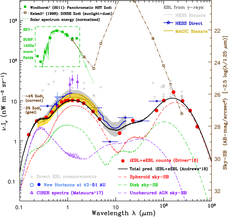
Much of the area surveyed with HST cameras consists of relatively empty sky surrounding targets of interest for which the observations were made. At 0.6–1.25 µm wavelength, over 95% of the photons in the HST Archive come from the Zodiacal Light in the InterPlanetary Dust (IPD) cloud, i.e., from distances less than 5 AU. This fraction is illustrated by the ratio of a typical ZL spectrum (green squares and green dotted line in Fig. 1) to the discrete EBL integral (red circles plus black model in Fig. 1, see also § 2.3). These photons are precisely the sky-SB photons present in nearly all HST images between the discrete objects that are of interest to our SKYSURF study. These sky photons come primarily from the ZL foreground, which is caused by sunlight scattered by dust and small particles in the IPD at distances r3–5 AU, or from even closer light sources such as Earthshine or Geocoronal emission, scattered light in the Optical Telescope Assembly (OTA) or thermal foregrounds in the camera detectors, as discussed in § 4 and SKYSURF-2. Constraints on ZL are obtainable from the HST Archive, yet no precise all-sky panchromatic measurements of the HST sky-SB exist. Ground-based telescopes are unable to make absolute measurements of the ZL due to atmospheric absorption, OH-lines, air glow, and light pollution unless very special measures are taken
2.2 Discrete HST Objects: Stars and Galaxies
Other than planetary and other moving targets, the main science interest in HST images has, in general, been stellar objects and galaxies from the brightest observable stars and star-forming (SF) regions in our own Galaxy and nearby galaxies to the faintest galaxies visible in the deepest HST images, such as the Hubble UltraDeep Field (HUDF, e.g., Beckwith et al., 2006). Stellar objects here will include Quasi-Stellar Objects (QSOs) or (weak) Active Galactic Nuclei (AGN). By selection, the large majority of objects observed in the HST Archive are nearly point-like objects. This is, of course, because HST was designed to observe faint objects at UV to red or near-IR wavelengths outside the Earth’s atmosphere (§ 1), and faint objects tend to be compact (the effects of SB-selection on the HST catalog completeness are discussed in § 4.7; see also Windhorst et al., 2008, 2021).
To date, the Hubble Legacy Archive (HLA) 222http://hla.stsci.edu contains over 1.5 million HST observations, and the Hubble Source Catalog (HSC) 333http://archive.stsci.edu/hst/hsc/ contains at least 3.7 million objects. Following the detailed description of Budavári & Lubow (2012) and Whitmore et al. (2016), the HLC Version 1 object catalogs are derived from subsets of the WFPC2, ACS/WFC, WFC3/UVIS, and WFC3/IR SourceExtractor source lists from the HLA data release version 10 (DR10). This incorporated cross-matching and relative astrometry of overlapping images to minimize offsets between closely aligned sources in different images. After correction for such offsets, the astrometric residuals of cross-matched sources are significantly reduced, with median errors less than 8 m.a.s. The absolute astrometry of the HLA is anchored into Gaia DR1, Pan-STARRS, the Sloan Digital Sky Survey (SDSS), and 2MASS.
The HLA and HLC are an outstanding permanent legacy of HST’s 30+ year record. SKYSURF’s main goal is not to replicate the extensive work that the HLA and HLC have done to create its object catalogs. Instead, SKYSURF focuses on the 249,861 ACS/WFC, WFPC2, WFC3/UVIS, and IR images in principle suitable for SKYSURF’s main sky-SB science goals, as discussed in § 2.5–4. Of these images, 220,657 have exposure times 200 sec, and are also eligible for drizzling, panchromatic object catalogs and object counts, as discussed in § 4.5–4.6 & Appendix B–C. Using the WFC3/IR F125W filter as the fiducial wavelength in this paper, two aspects are essential for SKYSURF:
(1) The Galactic star-counts have very flat slopes, while the galaxy counts have much steeper count slopes, and they cross over with about equal surface densities at average Galactic latitudes around AB18 mag at 1.25 µm (e.g., Windhorst et al., 2011, see also § 4.7 and its Figures here).
(2) The galaxy counts change from non-converging to converging slopes in the range 17AB22 mag with only a mild dependence on wavelength (Windhorst et al., 2011; Driver et al., 2016b). Therefore, while the vast majority of objects detected in HST images of average (1–2 orbits) depth are moderately faint (AB26 mag) galaxies, most of the total energy emitted by discrete objects at UV–optical–near-IR wavelengths is produced by those galaxies already detected in single-exposure HST images (Driver et al., 2016b, § 2.3 & 4.7 here).
The consequences of these two facts for SKYSURF are rather profound: to accurately measure both the integrated discrete galaxy counts and the sky-SB from all SKYSURF images, we must have: (a) very accurate star-galaxy separation procedures, especially at brighter fluxes (AB18 mag) where stars dominate the object counts; and (b) very accurate procedures to grow the light profiles of all detectable stars and galaxies, especially those with 17AB22 mag, where most of the EBL is produced, and remove their discrete object light from the images before the best estimates of the ZL and EBL can be made. Hence, SKYSURF must measure and account for the light from all discrete objects from 220,657 HST images in a manner that differs from that adopted for the HLA/HSC, as described below. For this, we will use the star-galaxy separation methods of Windhorst et al. (2011), which on shallow HST images are generally robust to AB25–26 mag (§ 4.7).
2.3 Integrated and Extrapolated Extragalactic Background Light from Discrete Objects (iEBL+eEBL)
The Extragalactic Background Light is defined as the flux received from all sources of photon production since recombination at far-UV (0.1 µm) to far-IR (1000 µm) wavelengths (e.g., McVittie & Wyatt, 1959; Partridge & Peebles, 1967a, b; Hauser & Dwek, 2001; Lagache et al., 2005; Kashlinsky, 2005; Finke et al., 2010; Domínguez et al., 2011; Dwek & Krennrich, 2013; Khaire & Srianand, 2015; Driver et al., 2016b; Koushan et al., 2021; Saldana-Lopez et al., 2021). That is, the EBL reflects the energy production of the Universe from z1090 until today and consists mainly of light from stars, AGN, and reprocessed light from dust, with some contribution from material heated by accretion (e.g., Alexander et al., 2005; Jauzac et al., 2011; Andrews et al., 2018). The EBL observed today thus results from the cosmic star-formation history, AGN activity (i.e., accretion onto super-massive black holes), and the evolution of cosmic dust over the past 13.5 billion years. The EBL can be divided into two roughly equal components: one covering the UV–near-IR (0.1–8µm; the Cosmic Optical Background, COB) and one covering the mid–far-IR (8–1000µm; the Cosmic Infrared Background, CIB; Dwek et al., 1998; Kashlinsky & Odenwald, 2000; Andrews et al., 2018; Fig. 1 here).
With the advent of space-based and ground-based facilities, deep fields have been obtained across the entire far-UV to far-IR wavelength range. For instance, Driver et al. (2016b) and Koushan et al. (2021) combined recent wide and deep panchromatic galaxy counts from the Galaxy And Mass Assembly survey (GAMA; Driver et al., 2011, 2016a; Hopkins et al., 2013; Liske et al., 2015), COSMOS/G10 (Davies et al., 2015; Andrews et al., 2017), the HST Early Release Science field (ERS; Windhorst et al., 2011), and Ultra-Violet Ultra-Deep Fields (UVUDF; Teplitz et al., 2013; Rafelski et al., 2015), plus near-, mid- and far-IR datasets from ESO, Spitzer and Herschel. To estimate the EBL from discrete objects, great care was taken in each dataset to produce object catalogs, total fluxes and object counts across a broad wavelength range.
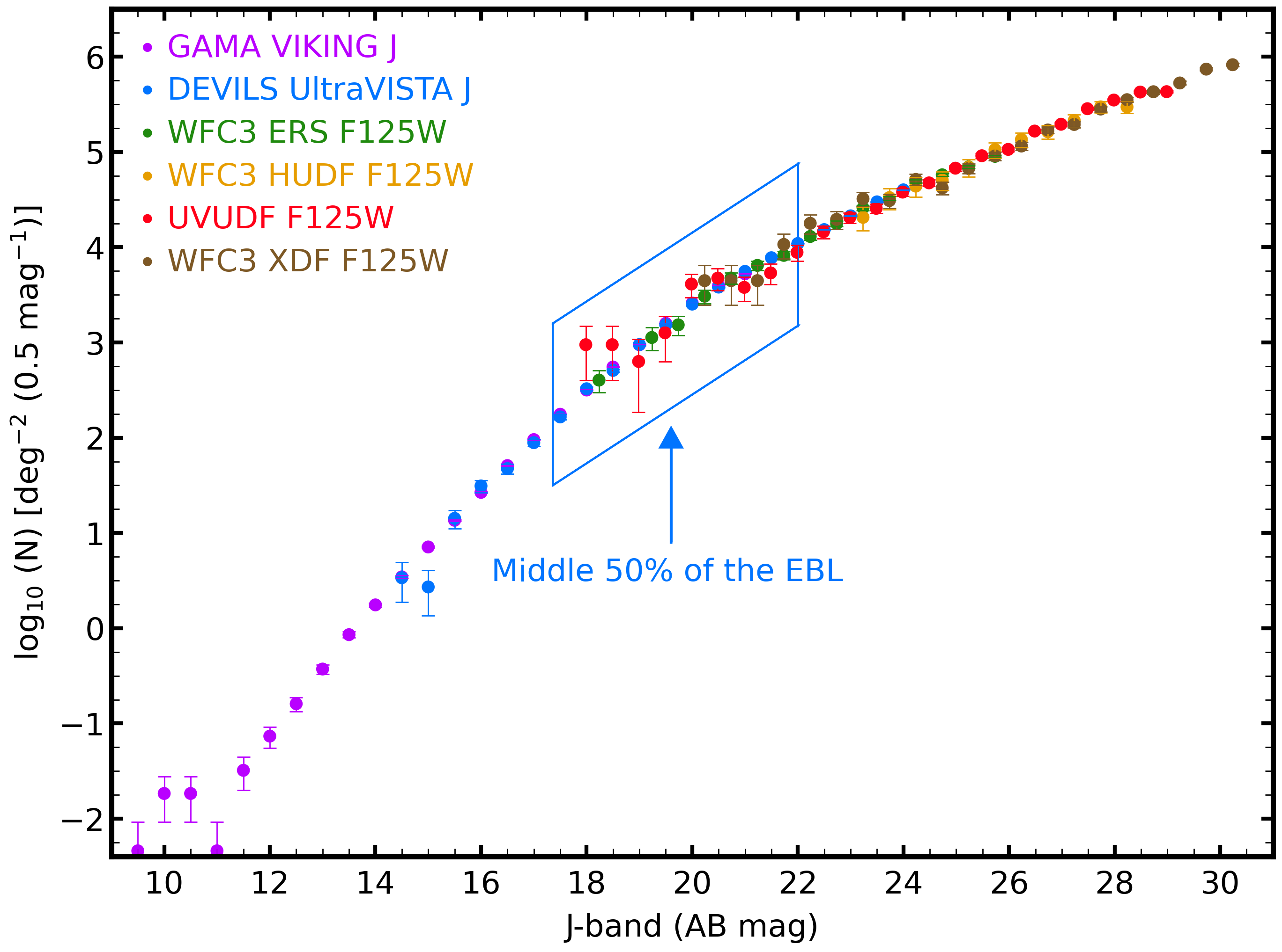
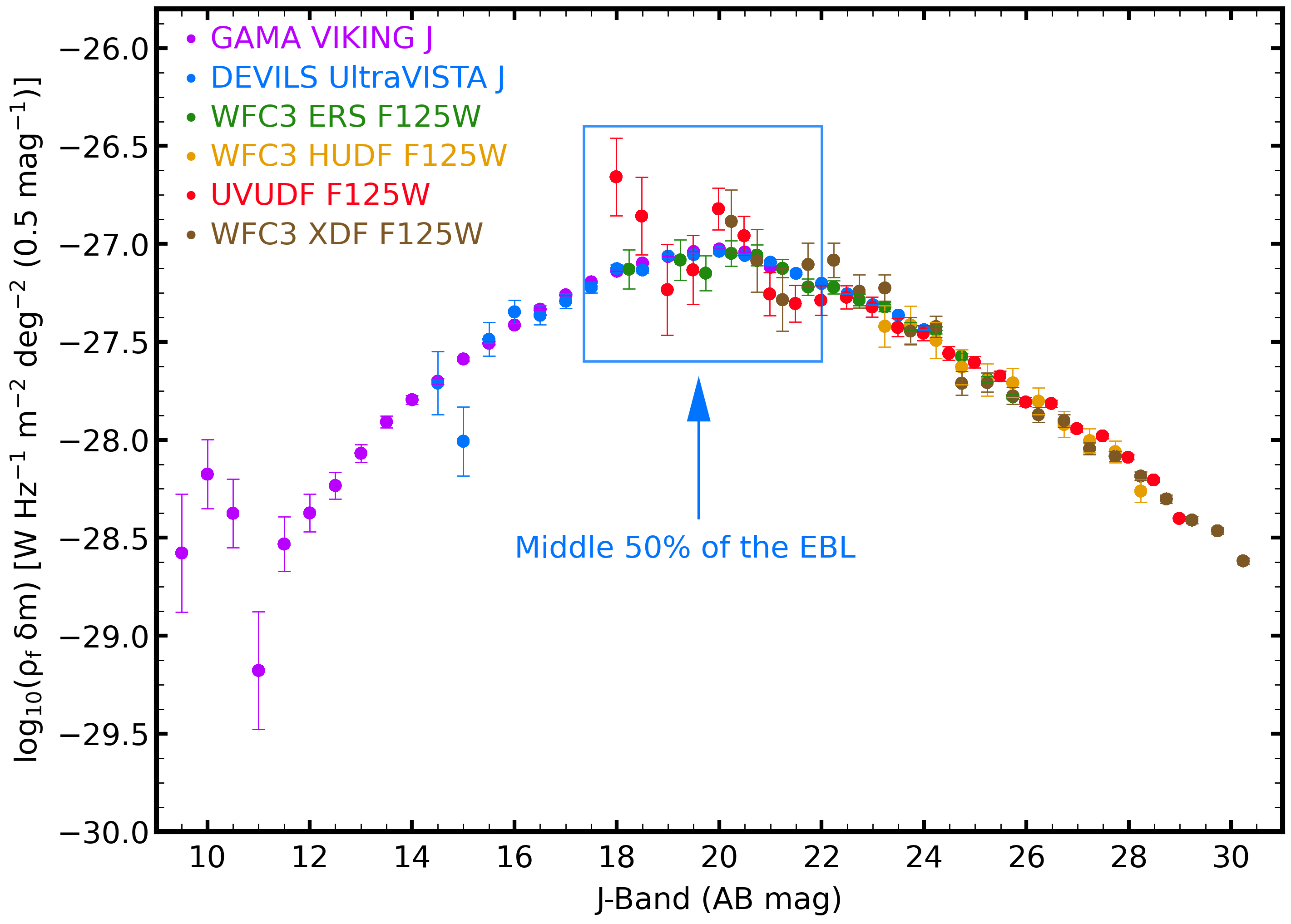
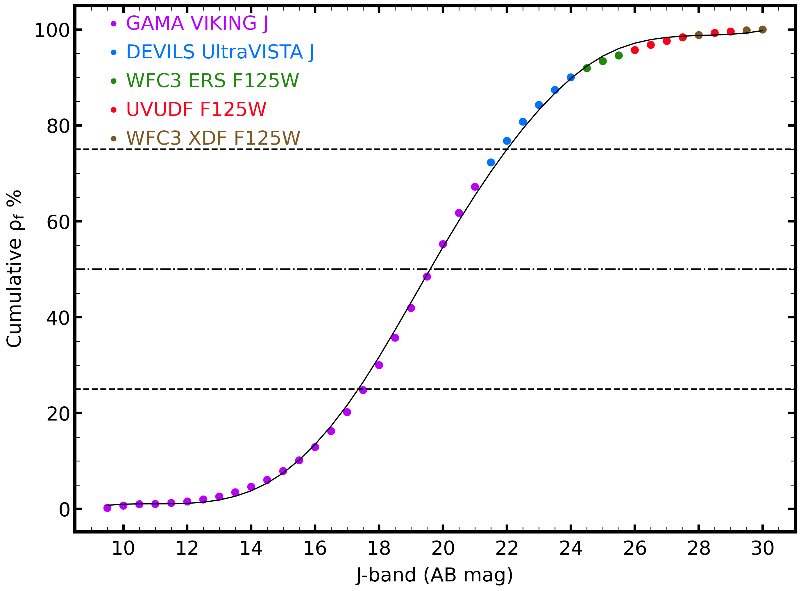
Fig. 2 gives an example of this process as relevant for the current SKYSURF analysis. Fig. 2a shows the galaxy counts in the J-band or F125W filter from the above datasets. Fig. 2b shows these galaxy counts normalized to the converging magnitude-slope of =0.40 (Driver et al., 2016b), which yields the EBL energy contribution .m from each 0.5 mag-wide flux interval. Earlier examples of the integrated galaxy counts and the resulting EBL are given by, e.g., Madau & Pozzetti (2000), Hopwood et al. (2010), Xu et al. (2005), Totani et al. (2001), Dole et al. (2006), Keenan et al. (2010), Berta et al. (2011), and Béthermin et al. (2012), as summarized in Driver et al. (2016b) and Koushan et al. (2021). The galaxy contribution to the integrated light is bounded since the faint galaxy count slope falls well below the critical value for convergence (i.e., = log N/m0.4).
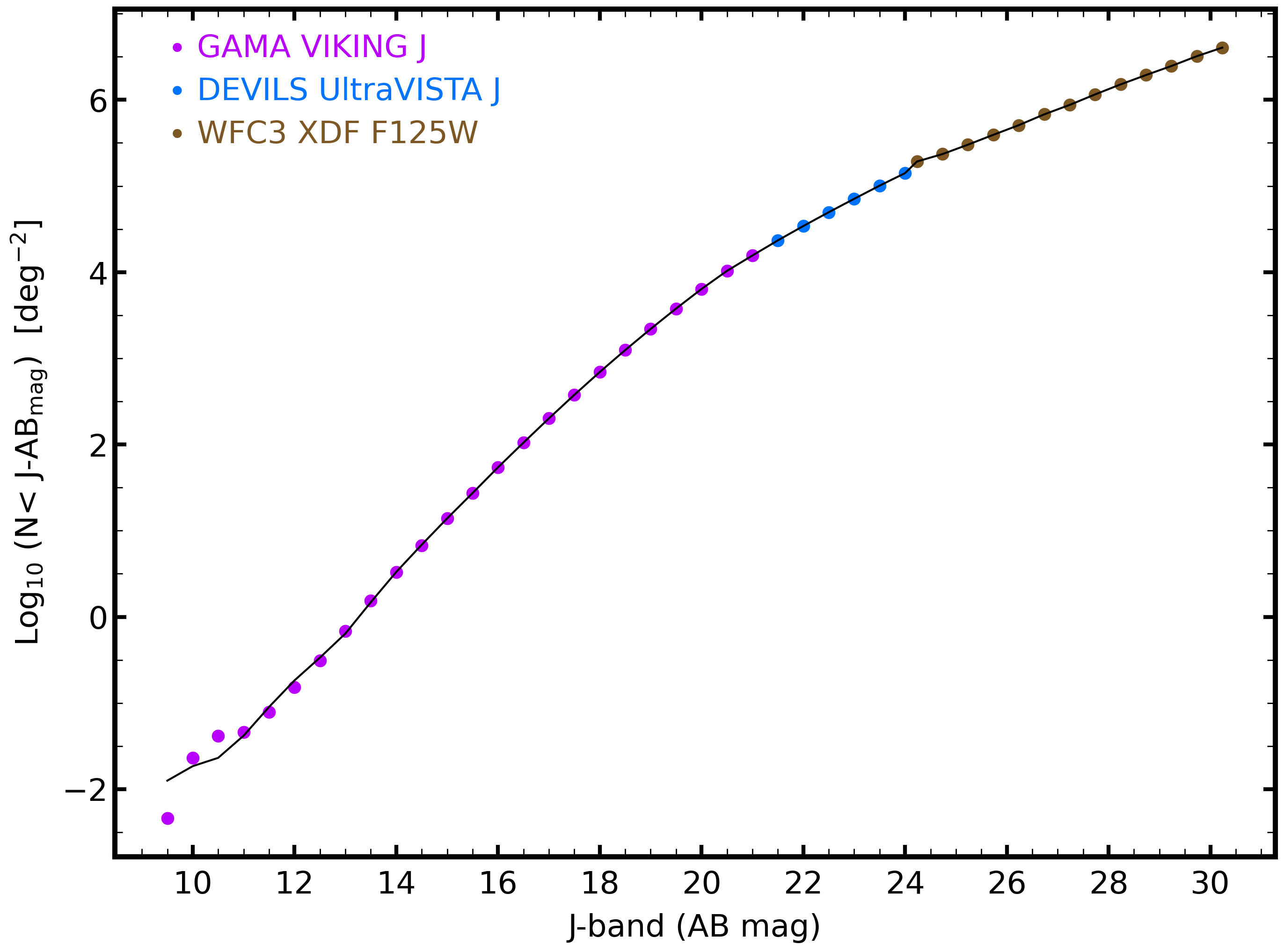
This integral over the discrete galaxy counts converging down to the detection limit is referred to as the “iEBL”, and the extrapolated converging integral of the discrete galaxy counts beyond the detection limit as the “eEBL” (Fig. 2bd). The discrete EBL is defined as the sum of the iEBL and eEBL, which is indicated by the red-filled circles in Fig. 1. The discrete EBL is distinct from the diffuse EBL which is defined in § 2.4.
Driver et al. (2016b) and Koushan et al. (2021) used Monte Carlo spline fits to extrapolate the observed discrete galaxy counts to beyond the detection limits of the deepest available images, which provided a range in allowed extrapolated slopes and corresponding uncertainties in the resulting eEBL. These simulations are consistent with the range in faint-end power-law slopes of the galaxy luminosity function over the relevant redshift range (e.g., Ilbert et al., 2005; Hathi et al., 2010; Windhorst et al., 2021), and result in eEBL integrals that, in general, converge very quickly for AB26 mag (Fig. 2b). The integrated discrete iEBL as extrapolated with the eEBL in Fig. 2d is thus an estimate of the discrete EBL that comes from galaxies. In § 4.7, we will correct the discrete eEBL for the fraction of fainter objects known to exist in deeper HST images that are missing due to SB-incompleteness effects in the shallower SKYSURF images. Fig. 1 also shows the 3-component EBL model prediction of Andrews et al. (2018) that links spheroid formation dominating at high-redshift to later disk formation and (unobscured) AGN, as well as reprocessing of UV photons by dust. The model predictions of Cowley et al. (e.g., 2019) match these iEBL+eEBL measurements.
Fig. 2d shows that the brightest 25% of the discrete iEBL comes from galaxies brighter than 17.36 mag, while the faintest 25% is due to galaxies fainter than 22.01 mag. The interquartile range of 17.36 22.01 mag — indicated by the blue boxes in Fig. 2ab, and by the corresponding blue wedges in the Figures of § 4.7 — accounts for the middle 50% of the discrete J-band iEBL and is due to galaxies with a median redshift z 1. Thus, most of the discrete iEBL flux comes from moderately faint galaxies already detected in short SKYSURF exposures at AB26 mag, where the change in count-slope occurs at all UV–optical–near-IR wavelengths.
2.4 Diffuse Extragalactic Background Light (dEBL)
The total EBL is defined as the sum of the integrated and extrapolated discrete EBL of § 2.3 and any diffuse EBL component that may exist:
| (1) |
Fig. 1 compares the discrete EBL (iEBL+eEBL) of Driver et al. (2016b, which they define as “eIGL”) from the far-UV to the far-IR to various total EBL estimates or upper limits as reviewed by Dwek & Krennrich (2013) and Ashby et al. (2015). Many of these methods estimate the total EBL directly, which are plotted as grey triangles (e.g., Puget et al., 1996; Fixsen et al., 1998; Dwek & Arendt, 1998; Hauser et al., 1998; Lagache et al., 1999; Dole et al., 2006; Bernstein et al., 2002; Bernstein, 2007; Cambrésy et al., 2001; Matsumoto et al., 2005, 2011). More recent work that constrained the absolute EBL level can be found in Matsuura et al. (e.g., 2011) for the far-IR CIB through AKARI measurements, in Tsumura et al. (2013), Matsuura et al. (2017) and Sano et al. (2020) for NIR EBL constraints, and in Kawara et al. (2017) and Mattila et al. (2017) for optical EBL constraints. Fig. 1 also shows the New Horizons constraints on diffuse light observed at 4.7–51 AU from the Sun (Zemcov et al., 2017; Lauer et al., 2021, 2022), where the ZL contribution is much smaller.
In the far-IR, the discrete EBL agrees fairly well with the directly measured CIB (Béthermin et al., 2012; Magnelli et al., 2013), but Fig. 1 shows a significant optical–near-IR discrepancy between the iEBL+eEBL data (red-filled circles) and the total EBL estimates (grey triangles). This difference amounts to as much as a factor of 3–5, and is often attributed to a possible component of diffuse Extragalactic Background Light (dEBL). We note that earlier groups plotted the total EBL signal (i.e., before the iEBL+eEBL was subtracted) in figures like Fig. 1, while more recent work did subtract the iEBL+eEBL from their data, either by modeling and subtracting it directly (e.g., Lauer et al., 2021, 2022), or by using CIBER spectra including the Ca-triplet to estimate and subtracting the Zodiacal foreground (e.g., Matsuura et al., 2017; Korngut et al., 2022). Hence, their Zodi+iEBL+eEBL subtracted diffuse light values have been plotted in Fig. 1. Our HST SKYSURF analysis in § 3–4 below already automatically subtracts from the diffuse light signal: a) almost all the starlight, b) 95% of the discrete EBL integral from objects detected in the HST images with AB26.5 mag; and c) estimates and subtracts the undetected eEBL integral for AB26.5 mag, which is 5% of the total discrete EBL in Carleton et al. (2022). Hence, our SKYSURF results will be directly comparable to these most recent results. We return to this point in § 5.
HESS/MAGIC -ray Blazar studies (e.g., Biteau & Williams, 2015; Dwek & Krennrich, 2013; H. E. S. S. Collaboration et al., 2013; Lorentz et al., 2015; Fermi-LAT Collaboration et al., 2018; grey and orange wedges in Fig. 1) provide independent constraints to the total EBL from deviations of the Blazar TeV spectra from a power-law, which is explained by pair-production involving -ray and EBL photons. Desai et al. (2019) and HAWC Collaboration (2022) similarly find low numbers based on GeV–TeV from Fermi-LAT and HAWC, respectively. Hence, -ray Blazar studies would imply a lower level of dEBL than these direct studies that constrain the total EBL.
Direct estimates of the true level of dEBL rely on a robust subtraction of three other sources of light: ZL, DGL, and the iEBL+eEBL (Hauser & Dwek, 2001; Mattila, 2006). SKYSURF is designed to investigate this apparent discrepancy between the total EBL signal and the discrete iEBL+eEBL. If real, this rather large discrepancy could be caused by a number of systematic errors that may result in larger foregrounds. In order of increasing distance from the HST instrument A/D converters, these are:
(1) Uncorrected systematics in the HST sky-SB measurements, e.g., detector systematics (§ 4.1) or Thermal Dark signal (SKYSURF-2);
(2) Close sources of straylight (e.g., Earthshine or scattered Sunlight; § 4.3);
(3) Systematic deviations from, or missing components in the ZL model (SKYSURF-2);
(4) Systematic deviations from and uncertainties in the DGL model (see references in SKYSURF-2, );
(5) Contributions by Intra-galaxy Halo Light (IHL) or (undetected) low SB galaxies (SKYSURF-2); and
(6) Diffuse light from Reionization (Windhorst et al. (e.g., 2018)).
Since we do not know the true cause of this discrepancy in Fig. 1, we will hereafter refer to light sources not accounted for by HST systematics, identifiable straylight, the ZL and DGL models or the discrete EBL more generally as “diffuse light” and not as “dEBL”. Further details on possible sources of diffuse light are given in SKYSURF-2.
In summary, most of the discrete EBL comes from moderately faint galaxies at 17AB22 mag in the redshift range 0.5z2. The true level and source of any diffuse light is as yet unclear. SKYSURF is designed to help reconcile the total EBL measurements with the integrated and extrapolated EBL (Fig. 1–2), and investigate how much room may be left for a truly diffuse light component, whatever its nature.
2.5 SKYSURF’s High-Level Project Outline
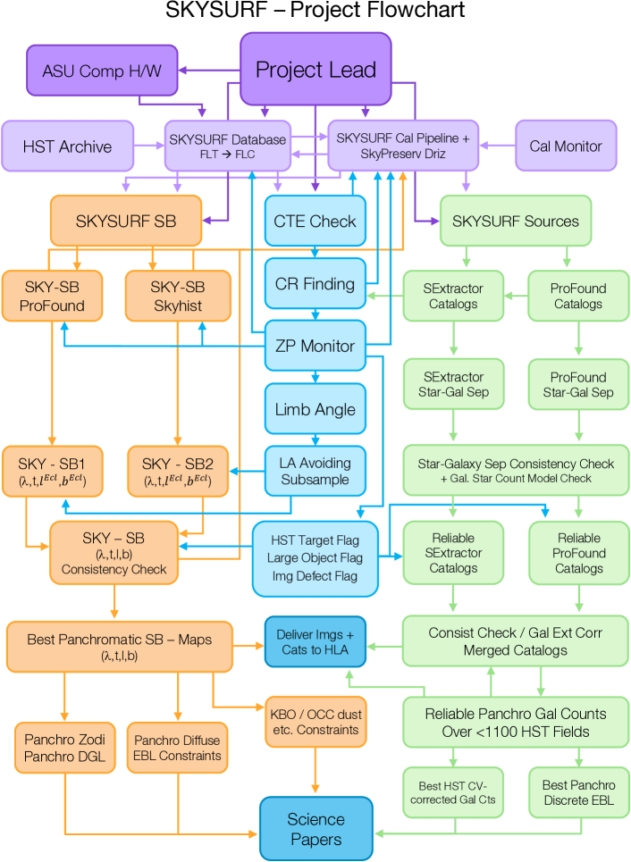
SKYSURF has two main science parts, and two essential supporting parts, as illustrated in the colored columns and rows in Fig. 3. We highlight both science parts briefly here, with details discussed in § 3–4.
2.5.1 SKYSURF-SB: All-Sky Constraints to ZL and DGL
As indicated by the orange columns in Fig. 3, SKYSURF will estimate the absolute sky-SB at 0.2–1.7µm using the methods of § 4. From 249,861 ACS+WFC3 images in the Archive, we select those with the lowest contamination due to Earthshine, Sun and Moon. The measured SB-values sample the entire sky and can be modeled as:
| (2) |
Here, ZL(t) and DGL can be fit simultaneously on scales of degrees as a function of wavelength, Ecliptic coordinates (, ), Galactic coordinates (, ), time of the year () or Modified Julian Date (MJD), and Sun Angle (SA), to match SKYSURF’s very large number of panchromatic sky-SB measurements. The time- or SA-dependence is the key factor that distinguishes the ZL from other SB components. The HST data do not sample the temporal and spatial parameter space as deeply and uniformly as the COBE/DIRBE data (e.g., Kelsall et al., 1998), but the HST sky-SB data do sample a wider range of solar elongations and cover a full calendar year (multiple times). The TD parameter on the right-hand side is the WFC3/IR Thermal Dark signal that depends on wavelength and HST’s ambient temperature . This near-IR thermal component needs to be modeled and subtracted from any diffuse light signal that we observe (§ 4.1.4 and SKYSURF-2, ). The SL parameter indicates the straylight that the HST telescope + instruments receive from the Earth, the Sun and the Moon, which we attempt to minimize using the methods in § 4.3 and SKYSURF-2 when assessing our constraints on the ZL, DGL and EBL. The SL depends on wavelength and time or orbital phase, which determines the angles to the Earth’s Limb, Sun and Moon (§ 4.3).
In SKYSURF-2, we will identify any large differences between the HST sky-SB measurements and existing ZL models, which is most straightforwardly done at wavelengths 1.25–1.6 µm as a function of Ecliptic Latitude . A major goal of SKYSURF is to update the ZL models to cover the full 0.2–1.7 µm wavelength range observed by SKYSURF, and the range of (, ) and SA values sampled by HST.
2.5.2 SKYSURF-Sources: Panchromatic Counts and iEBL/eEBL Averaged over Cosmic Variance
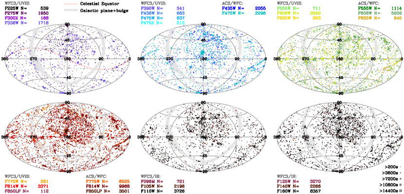
The discrete panchromatic object counting part of SKYSURF is indicated by the green columns in Fig. 3, which provides discrete object catalogs, star-galaxy separation, and object counts in the main HST broad-band filters across the sky. Because the normalized differential galaxy counts flatten with a converging slope for AB22 mag (Fig. 2b), most of the EBL-energy (and its uncertainty) comes from galaxies with AB17–22 mag at a median redshift z1. Their Cosmic Variance (CV) over a single HST FOV is 30–40% at these redshifts (e.g., Somerville et al., 2004; Trenti & Stiavelli, 2008; Moster et al., 2011; Driver et al., 2016b). SKYSURF’s goal is therefore to average the panchromatic galaxy counts over 1400 well-separated representative HST fields to reduce the iEBL-errors from cosmic variance to 2%, or 4% when accounting for the systematic and zeropoint errors in § 4.1.5. Even a contiguous HST survey region of 1400 fields (e.g., COSMOS) would still give 8% CV, and such fields are not available in the 12 main broad-band HST filters. Hence, SKYSURF’s all-sky distribution of the 1400 independent HST fields in Fig. 4 is essential to reduce CV in the resulting galaxy counts (Driver & Robotham, 2010). Further details are given in § 3.2, 4.5 and Tompkins et al. (2022, in preparation).
In what follows, we will define independent HST fields as those instrument FOVs that are far enough apart in the sky (1∘) to provide faint galaxy counts that are sufficiently independent to average over CV. Fig. 4 shows that there are 4,858 independent HST FOVs using this definition, not all of which are usable for objects counts (§ 3.2 & Appendix B.3). As discussed in § 3, the total number of instrument FOVs that SKYSURF has covered is 3.5 larger, as many HST users have covered their targets on average by a number of adjacent instrument FOVs.
To the typical 5 completeness limits of AB26–28 mag of most drizzled SKYSURF images we expect an integrated galaxy surface density of (3–5)105 deg-2 (e.g., Fig. 2ac). For the estimated total usable SKYSURF area of 10 deg2 (§ 3.2), this implies a total of (3–5)106 galaxies. Hence, SKYSURF will provide galaxy counts for a sample as large as the SDSS (York et al., 2000), but distributed over the whole sky and reaching 5 mag deeper. Unlike SDSS, the SKYSURF discrete object sample does not cover a contiguous area. But because it sparsely samples the whole sky, SKYSURF’s discrete object catalogs will be well suited to minimize Cosmic Variance in the galaxy counts. A key element of this SKYSURF goal is HST’s photometric stability over 11–18 years of data (§ 4.1.5).
2.5.3 SKYSURF Plan
Because the SKYSURF database contains 249,861 HST Archival images, it does, in general, not lack sufficient statistics, not even after conservative removal of large foreground targets and image defects (Appendix B.3). Instead, SKYSURF is limited by systematic errors, and for this reason, we need to carefully account for possible systematics summarized in § 4. Hence, SKYSURF carries out each of its two main science goals — accurate panchromatic sky-SB measurements and object counts — along two main independent paths each, indicated by the two orange and two green columns in Fig. 3 with significant cross-checks. The purple rows in Fig. 3 show SKYSURF’s database building and its data processing (§ 3–4), while the blue column shows its specific data flagging steps (§ 4 and Appendix B.3).
3 Project SKYSURF — Database Overview
In this section, we summarize the selection of the SKYSURF instruments, filters, and exposures (§ 3.1), and the resulting SKYSURF database and total usable survey area (§ 3.2). The database considered for SKYSURF ranges from each instrument’s launch date until January 2020, when we started building its database. Summaries of each HST instrument used in SKYSURF and their data reduction pipelines can be found in the Instrument Handbooks (IHBs), Data Handbooks (DHBs), and Instrument Science Reports (ISRs) listed on the STScI website 444https://www.stsci.edu/hst/instrumentation. Specific HST instrument details relevant for SKYSURF are discussed in § 4.1.
3.1 SKYSURF Instruments, Filters, and Exposures
HST Instruments Used: SKYSURF’s Archival data come from HST’s primary wide field imaging instruments: ACS/WFC, WFPC2, WFC3/UVIS and WFC3/IR. These data span more than 17 years for ACS (2002–2020), 16 years for WFPC2 (1994-2009), and 11 years for WFC3 (2009–2020). Despite its much older detectors, broad-band WFPC2 images were included in SKYSURF because they provide an earlier time baseline (1994–2009). ACS/WFC and WFC3/UVIS have higher throughput than WFPC2, but due to its much larger pixels WFPC2’s sensitivity to SB is comparable to that of ACS/WFC and WFC3/UVIS. For many targets WFPC2 provides broad-band exposures in the common “BVI” filters (F555W, F606W, and F814W) that were later replicated in the same filters with ACS/WFC or WFC3/UVIS. Hence, we will compare the older WFPC2 sky-SB estimates for the same targets observed at the same time of the year (i.e., at similar Sun Angles) to those observed later in the same filters with ACS/WFC or WFC3/UVIS. This provides SKYSURF with an independent assessment of subtle instrument systematics in the sky-SB measurements and zeropoint drifts over the decades. Details are given in O’Brien et al. (2022, in preparation).
WFPC2, ACS/WFC, and WFC3/UVIS+IR Images not used in SKYSURF: We did not retrieve from the HST Archive all of the following ACS/WFC, WFPC2 and WFC3/UVIS and WFC3/IR image types for SKYSURF: (1) grism, narrow-band and most medium-band images; (2) images taken with Quad or Linear Ramp filters; (3) images that use subarrays or time-series; (4) images of (fast) moving targets; (5) WFC3/UVIS or WFC3/IR images that were produced by spatial scans; and (6) ACS polarization images where a Polarizer is crossed with a broad-band filter. This is because these images are harder to calibrate and because their sky-SB would be much harder to measure, since it may not be uniform across these specialized images by their very design.
Other HST Cameras not used in SKYSURF: The following other HST cameras have been onboard the HST spacecraft part of the last 32 years, but are not used for SKYSURF: WF/PC-1, FOC, ACS/HRC & SBC, NICMOS NIC1, NIC2, NIC3, STIS/CCD, and STIS/MAMA. For WF/PC-1, this is because the instrument was in HST’s spherically aberrated beam, which affects both point source detection and accurate SB-measurements (e.g., Windhorst et al., 1992, 1994a). The ACS/HRC & SBC, FOC, NICMOS NIC1, NIC2, NIC3, STIS/CCD, and STIS/MAMA images are not used, because they cover very small FOVs, and/or have rather unusual or very broad-band filter sets that would be hard to compare to measurements in the standard modern filter sets present in ACS/WFC, WFPC2, or WFC3. NICMOS also has significant time-dependent dark-current levels (the “pedestal” effect) that would make dark-current subtraction and absolute sky-SB measurements rather uncertain, despite the advantage of significantly lower foregrounds in the near-IR over the other early HST instruments.
SKYSURF Pointings: The HST pointings used for SKYSURF are not completely randomly distributed across the sky (Fig. 4). They are sparser in the South than in the North, with a tendency to avoid the Galactic plane (20∘) and favoring the celestial equator (Decl.0∘). These biases can be due to, e.g., HST observers selecting targets from ground-based surveys in equatorial regions that can be accessed by ground-based telescopes in both hemispheres, and from the SDSS whose footprint is clearly visible through its higher density of HST targets in Fig. 4 (see § 3.2).
SKYSURF Filters: We use the 12 main broad-band filters between 0.2–1.7 µm (UV [F225W]–H [F160W]). Fig. 4 shows that SKYSURF has 28 broad-band ACS and WFC3 filters in total. Many of these filters are very similar in wavelength and may be grouped together (after small zeropoint corrections and differential K-corrections; see Windhorst et al., 2011) when combining them into the panchromatic galaxy counts. All 28 filters will be used for panchromatic sky-SB determination at their appropriate effective wavelengths (), but the galaxy counts may be combined in very similar filters. Filter red leaks and blue leaks are discussed in § 4.1.
Wide Field Planetary Camera 2 data since 1994: The main SKYSURF filters used for WFPC2 are the F300W, F336W, F439W, F450W, F555W, F606W, F675W, F702W, F814W, and F850LP filters, plus several other less-used broad-band filters summarized in Table 1.
Advanced Camera for Surveys/Wide Field Channel data since 2002: The main SKYSURF filters used for the ACS/WFC are the F435W, F475W, F555W, F606W, F775W, F814W, and F850LP filters, also broadly referred to as the ACS “” filters, plus several other less-used broad-band filters summarized in Table 2a.
Wide Field Camera 3 UVIS data since 2009: The main SKYSURF filters used for WFC3/UVIS are the vacuum UV filters F225W, F275W, F336W, and the F438W, F555W, F606W, and F814W, filters, also broadly referred to as the WFC3 “” filters, plus several other less-used broad-band WFC3/UVIS filters, including F775W and F850LP, summarized in Table 2b. Where possible, these WFC3/UVIS filters are used as external checks on the ACS/WFC sky-SB values measured in the same filters on the same targets observed at similar times of the year.
Wide Field Camera 3 IR data since 2009: The main SKYSURF filters used for WFC3/IR are the F098W, F105W, F110W, F125W, F140W, and F160W filters, as summarized in Table 3, plus several other less-used medium-band or narrow-band filters used for the WFC3/IR Thermal Dark signal calibration in SKYSURF-2.
SKYSURF Exposures and Exposure times: We initially considered all ACS/WFC, WFPC3, WFC3/UVIS and WFC3/IR exposures for SKYSURF processing, regardless of whether or not the LOW-SKY or SHADOW Special Requirements were specified by the HST observer in the Astronomers Proposal Tool (“APT” 555https://www.stsci.edu/scientific-community/software/astronomers-proposal-tool-apt). For sky-SB measurements we sub select exposures of sufficient duration to allow robust estimates of the background level. For drizzling and discrete object catalog generation, we sub select images with exposure times 200 sec, which constitute the vast majority of images and ensures sufficient depth for our purposes. These are generally the exposures where the sky-noise exceeds the read-noise (except in the UV due to significant Charge Transfer Inefficiency trails; see § 4.1 & Appendix B.2), and so they are potentially the most useful for galaxy counts over as large of a random area as possible. As an example, the distribution of exposure times for all 6796 WFC3/IR F125W images available to SKYSURF is shown in Fig. 5. The median exposure time is 500 sec, where a typical F125W image reaches AB 26 mag (5) for compact objects. In general, comparable median exposure times are found for SKYSURF’s other broad-band filters listed in Tables 1–3. These Tables also list the corresponding median image depths derived from the instrument Exposure Time Calculators.
| Instr/ | NExp | Disk | NExp | -limit | -limit | -limit | ||||||
|---|---|---|---|---|---|---|---|---|---|---|---|---|
| Filter | Space | — only sec — | — for all — | — for images with all — | ||||||||
| (GB) | (s) | (s) | (s) | (s) | (s) | (s) | (AB-mag) | (AB-mag) | (AB-mag) | |||
| WFPC2 | ||||||||||||
| F255W | 796 | 97.0 | 796 | 500 | 300 | 800 | 500 | 300 | 800 | 22.54 | 22.00 | 23.03 |
| F300W | 11019 | 97.0 | 10744 | 800 | 400 | 1000 | 800 | 400 | 1000 | 25.17 | 24.44 | 25.40 |
| F336W | 2514 | 22.0 | 2134 | 600 | 400 | 900 | 600 | 400 | 1000 | 24.71 | 24.28 | 25.24 |
| F380W | 89 | 0.8 | 89 | 600 | 500 | 1000 | 600 | 500 | 1000 | 25.16 | 24.98 | 25.67 |
| F439W | 1298 | 12.0 | 1298 | 500 | 313 | 700 | 500 | 313 | 700 | 24.65 | 24.16 | 24.99 |
| F450W | 5991 | 84.0 | 5988 | 600 | 400 | 1000 | 600 | 400 | 1000 | 25.90 | 25.51 | 26.36 |
| F547M | 611 | 5.3 | 611 | 400 | 300 | 600 | 400 | 300 | 600 | 25.25 | 24.97 | 25.63 |
| F555W | 6829 | 59.0 | 6457 | 500 | 350 | 1100 | 600 | 350 | 1200 | 26.34 | 25.88 | 26.88 |
| F569W | 44 | 0.37 | 44 | 800 | 500 | 1100 | 800 | 500 | 1100 | 26.37 | 25.97 | 26.62 |
| F606W | 24265 | 205.0 | 24168 | 600 | 500 | 1000 | 600 | 500 | 1000 | 26.63 | 26.49 | 27.00 |
| F622W | 186 | 1.6 | 186 | 900 | 600 | 1000 | 900 | 600 | 1000 | 26.57 | 26.25 | 26.65 |
| F675W | 1926 | 17.0 | 1822 | 500 | 400 | 700 | 500 | 400 | 700 | 25.90 | 25.71 | 26.17 |
| F702W | 2006 | 17.0 | 2000 | 700 | 400 | 1200 | 700 | 400 | 1200 | 26.47 | 26.03 | 26.86 |
| F785LP | 274 | 2.4 | 274 | 500 | 500 | 500 | 500 | 500 | 500 | 25.01 | 25.01 | 25.01 |
| F791W | 478 | 4.1 | 471 | 350 | 260 | 600 | 375 | 260 | 600 | 25.33 | 25.00 | 25.73 |
| F814W | 18759 | 160.0 | 18659 | 600 | 400 | 1100 | 600 | 400 | 1100 | 25.86 | 25.52 | 26.33 |
| F850LP | 1002 | 8.8 | 1002 | 400 | 400 | 600 | 400 | 400 | 600 | 24.17 | 24.17 | 24.57 |
| Subtot | 78087 | 793 | 76743 | |||||||||
| Instr/ | NExp | Disk | NExp | -limit | -limit | -limit | ||||||
|---|---|---|---|---|---|---|---|---|---|---|---|---|
| Filter | Space | — only sec — | — for all — | — for images with all — | ||||||||
| (GB) | (s) | (s) | (s) | (s) | (s) | (s) | (AB-mag) | (AB-mag) | (AB-mag) | |||
| ACS/WFC | ||||||||||||
| F435W | 5898 | 1250 | 5461 | 661 | 500 | 1200 | 650 | 440 | 1200 | 26.09 | 25.71 | 26.66 |
| F475W | 6280 | 1380 | 5417 | 522 | 370 | 700 | 470 | 365 | 674 | 26.12 | 25.89 | 26.46 |
| F555W | 2555 | 560 | 2317 | 540 | 385 | 700 | 520 | 370 | 697 | 25.88 | 25.55 | 26.15 |
| F606W | 16930 | 3730 | 15990 | 530 | 400 | 784 | 515 | 382 | 767 | 26.50 | 26.25 | 26.82 |
| F625W | 1839 | 380 | 1479 | 532 | 382 | 600 | 467 | 340 | 577 | 25.89 | 25.60 | 26.08 |
| F775W | 8953 | 2000 | 8675 | 510 | 404 | 716 | 503 | 400 | 608 | 25.70 | 25.48 | 25.87 |
| F814W | 30278 | 6710 | 27536 | 525 | 450 | 800 | 509 | 400 | 752 | 25.90 | 25.68 | 26.22 |
| F850LP | 8884 | 2000 | 8586 | 507 | 400 | 675 | 500 | 400 | 669 | 24.65 | 24.43 | 24.92 |
| Subtot | 81617 | 18010 | 75461 | |||||||||
| WFC3/UVIS | ||||||||||||
| F225W | 1600 | 280 | 1126 | 560 | 400 | 700 | 516 | 368 | 699 | 25.23 | 24.89 | 25.54 |
| F275W | 5622 | 920 | 3975 | 660 | 484 | 1212 | 528 | 190 | 800 | 25.24 | 24.20 | 25.65 |
| F300X | 366 | 61 | 141 | 609 | 351 | 869 | 450 | 100 | 600 | 25.87 | 24.37 | 26.14 |
| F336W | 4616 | 970 | 3999 | 645 | 470 | 820 | 600 | 408 | 800 | 25.91 | 25.52 | 26.19 |
| F390W | 1038 | 230 | 912 | 597 | 558 | 850 | 596 | 482 | 790 | 26.43 | 26.22 | 26.65 |
| F438W | 1851 | 260 | 1009 | 430 | 350 | 783 | 350 | 205 | 511 | 25.41 | 25.26 | 25.73 |
| F475W | 1977 | 240 | 905 | 800 | 400 | 1308 | 325 | 150 | 720 | 26.05 | 25.37 | 26.67 |
| F475X | 525 | 80 | 309 | 524 | 360 | 798 | 300 | 175 | 580 | 26.45 | 25.87 | 26.76 |
| F555W | 2271 | 350 | 1334 | 477 | 378 | 600 | 356 | 140 | 531 | 26.04 | 25.24 | 26.36 |
| F606W | 7794 | 1350 | 5484 | 599 | 400 | 843 | 425 | 300 | 700 | 26.37 | 26.11 | 26.71 |
| F625W | 804 | 100 | 425 | 515 | 400 | 700 | 370 | 180 | 621 | 25.85 | 25.27 | 26.26 |
| F775W | 688 | 170 | 279 | 606 | 400 | 699 | 320 | 200 | 507 | 25.23 | 24.90 | 25.56 |
| F814W | 10602 | 1880 | 6467 | 595 | 400 | 867 | 400 | 242 | 653 | 25.56 | 25.15 | 25.91 |
| F850LP | 330 | 50 | 192 | 374 | 364 | 473 | 349 | 200 | 379 | 24.42 | 23.87 | 24.49 |
| Subtot | 40084 | 6941 | 26557 | |||||||||
+ Instr/ NExp Disk NExp -limit -limit -limit Filter Space — only sec — — for all — — for images with all — (GB) (s) (s) (s) (s) (s) (s) (AB-mag) (AB-mag) (AB-mag) WFC3/IR F098M 1158 7 1103 703 603 1003 703 553 1003 25.98 25.80 26.23 F105W 5412 33 4792 603 299 903 403 228 803 25.98 25.53 26.46 F110W 8847 54 6473 353 253 603 288 203 503 26.08 25.82 26.47 F125W 6810 39 5554 553 453 703 503 299 653 26.06 25.68 26.24 F140W 5647 35 4691 349 228 603 299 203 553 25.80 25.49 26.24 F160W 22199 140 19283 503 399 653 453 303 603 25.69 25.38 25.89 Subtot 50073 308 41896 Total 249861 26052 220657 aafootnotetext: Detection limit is the AB-magnitude for 5 point sources at the median (50%) exposure time listed. The 25% and 75% columns indicate the exposure times and corresponding 5 point source detection limits for the shallowest 25% and 75% of the images, respectively. The last row gives the grand total over Tables 1–3.

3.2 The Panchromatic SKYSURF HST Database and Total Usable Area
Number of Exposures and Retrieval: We retrieved from the HST Archive all 249,861 available images (81,617 ACS/WFC + 78,087 WFPC2 + 40,084 WFC3/UVIS + 50,073 WFC3/IR exposures), or 26 TB in total (Fig. 4 and Tables 1–4). These images are all public as of 2020, and have exposure times up to one full orbit. Since processing and retrieval of such a vast amount of data posed some demands on the HST Archive, we spread ingestion over the Spring of 2020 with a typical transfer rate of 175 GB per day. Complete disk copies of the SKYSURF database are kept at ASU in Arizona and at ICRAR at the University of Western Australia.
All-Sky Maps of Available Panchromatic SKYSURF Images: All-sky maps of all images eligible for SKYSURF analysis are shown in Fig. 4a–4f. The SDSS footprint appears as the better-sampled tilted rectangle in Fig. 4, since the SDSS has provided many targets for HST survey and SNAPshot programs, and many of those images are suitable for SKYSURF. In our all-sky sky-SB analysis, SKYSURF will appropriately weigh the uneven sampling of panchromatic sky-SB values due to this higher HST field-density inside the SDSS footprint (Eq. 2), as well as the resulting all-sky discrete object counts over 1400 independent HST fields (§ 4.5 & Appendix C), as needed.
Estimated Total Usable SKYSURF Area: Table 4 summarizes the total number of exposures per SKYSURF instrument, to estimate the maximum usable area that HST has covered with these data since 1994. Each instrument uses between 1–3 detectors per camera, and Col. 5 lists the total number of SKYSURF single exposures of the full cameras (except for WFPC2 where the PC1 data were discarded). Col. 3 lists the FOV (in arcsec) for each of the full camera exposures, and Col. 4 the total area per full exposure in each camera. Col. 6 lists for each camera the approximate average number of exposures per filter and the approximate average number of filters used on each HST pointing, as well as their product. Since 1994, the average HST user of WFPC2, ACS, or WFC3 has used an average of 8 exposures per filter and 1.8 filters per pointing. The total number of filters per FOV ranges from 1 for single-exposure SNAPshot targets to 13 for the HUDF. Col. 7 lists the estimated number of independent HST pointings or FOVs in each full camera, which are considered those that are more than 1.0 FOV (or 6′) apart in their pointing centers, given the single detector FOV values in Col. 3. In § 4.5 we discuss how the drizzle footprints were defined that determined these associations. Col. 8 lists the maximum SKYSURF area covered by each camera, which is not yet corrected for repeat visits of a given pointing with a different camera in the same filter. This will be done when the footprints and drizzling of all SKYSURF data are finished on AWS (§ 4.5–4.6). Hence, only an upper limit to the total unique SKYSURF area is listed that may be usable for independent object counts across the sky.
Of the 249,861 individual exposures in the SKYSURF database, 220,657 images have 200 sec and are spread out over 16,822 HST pointings or FOVs across the sky (Fig. 4). The 249,861 SKYSURF exposures from Tables 1–3 contain 878,000 individual detector read-outs, including the 50,073 WFC3/IR exposures which we split into their individual ramp-readouts to better monitor sky-SB vs. orbital phase (§ 4.3). All 249,861 SKYSURF exposures are processed through the initial SB-measurement steps of § 4.2, as it cannot be determined a priori whether they are useful for SKYSURF’s sky-SB goals or not. We estimate that about one-third of all these images have LOW-SKY or SHADOW flags or equivalent low background levels, such that they can constrain the ZL, DGL, or any diffuse light.
The subset of 220,657 images with 200 sec is used for drizzling, object catalogs and counts, and has covered 32 deg2 across the sky since 1994 (Table 4). Of this total area, not all images are usable for SKYSURF background object counts, e.g., due to large targets that overfill the FOV, Galactic plane targets, or large artifacts (Appendix B.3). We estimate that about 30–50% of these 16,822 HST FOVs or 10 deg2 are in principle usable for object counts. In total, 4,858 of the 16,822 HST FOVs are 1∘ away from the nearest-neighbor HST field. Here, we assume that angular distances 1∘ at z1–2 — which corresponds to 30 Mpc in Planck Cosmology (Planck Collaboration et al., 2016) — make the galaxy counts in such fields sufficiently independent to average over CV (Driver & Robotham, 2010). Of these 4,858 independent FOVs, we also expect 30–50% to survive the large target or large defect filtering above, so we expect that 1400 of these HST targets can be meaningfully used to reduce CV in the galaxy counts. Henceforth, we refer to these as our “1400 independent HST fields” suitable for galaxy counts.
| SKYSURF | Nchipb | FOV | Area/Exp | NExp | NExp/Filt | NFOVd | Max. Total |
|---|---|---|---|---|---|---|---|
| Instrument | /chip | (arcm2) | NFilt/Pointc | Area (deg2)e | |||
| (1) | (2) | (3) | (4) | (5) | (6) | (7) | (8) |
| WFPC2a | 3 | 75′′75′′ | 4.69 | 76,743 | 6.011.7710.61 | 7,230 | 9.42 |
| ACS/WFC | 2 | 202′′101′′ | 11.33 | 75,461 | 9.391.7016.00 | 4,717 | 14.85 |
| WFC3/UVIS | 2 | 162′′81′′ | 7.29 | 26,557 | 6.241.9211.97 | 2,219 | 4.49 |
| WFC3/IR | 1 | 136′′123′′ | 4.65 | 41,896 | 8.861.7815.77 | 2,656 | 3.43 |
| Total SKYSURFf | 7.27 | 220,657 | 7.741.7713.65 | 16,822 | 32 |
4 High-level SKYSURF Methods
In this section, we discuss our methods to produce both sky-SB measurements and object catalogs from SKYSURF’s images, with the details needed to assess their accuracy, reliability and completeness across the sky. This includes the calibration methods applied, the image zeropoints (ZP) and ZP monitors as a function of time, our algorithms to make object-free estimates of the sky-SB, the orbital sky-SB dependence and sources of straylight, and our treatment of sky-SB gradients. Because SKYSURF’s object catalogs affect our estimates of the object-free sky-SB, we also summarize SKYSURF image drizzling strategy and drizzle footprints, as well as our star-galaxy separation method and catalog reliability and completeness.
4.1 Calibration with Best Available Calibration Files, and Other General Calibration Aspects
In this section, we summarize the standard calibration of all SKYSURF images with the best available calibration files and other calibration considerations for SKYSURF’s specific purposes. This includes any sources that systematically add or remove electron () signal from the image sky-SB levels, as well as the zeropoints and ZP monitoring over time of each HST instrument from which data is used here. This first sub-section discusses the effects that all instruments have in common, while the following sub-sections discuss specific aspects of each individual HST instrument as they may affect SKYSURF’s sky-SB measurements.
The relative sky-SB errors induced by each of the main aspects of the calibration process below are summarized in Table 5 as a percentage of the average sky-SB levels measured, with references to the sections below where details are given. All errors are 1- compared to the mean trends in the calibration parameters discussed in or estimated from the ISRs or IHBs cited below. In some cases, a range is given for the relative errors which may depend on wavelength or the presence of image gradients. The bottom row of Table 5 lists the total relative error in each of the instrument sky-SB estimates, which assumes that the individual error components are independent. When an error range is listed, the largest of the percentage errors are propagated into the total error. Hence, we consider the total relative sky-SB errors to be conservative estimates.
Standard calibration: SKYSURF calibrates each image using the latest on-orbit reference files and flux scale, which includes the standard bias-subtracted, dark-frame subtracted, flat-fielded images (the files), which have also been CTE-corrected (the files). The total of 249,861 images from Tables 1–3 were retrieved from the Mikulski Archive for Space Telescopes (MAST 666https://archive.stsci.edu) in Jan-May 2020 using the pipelines in effect as of that time period. For ACS these are the calacs pipeline version 10.2.1, and for WFC3 the calwf3 pipeline version 3.5.0. The WFC3/UVIS images were downloaded again in early 2022 calibrated with calwf3 pipeline version 3.6.2 to implement the 2021 CTE corrections (Appendix B.2) and to automatically correct for the slowly time-varying filter zeropoints as a function of wavelength (§ 4.1.5). O’Brien et al. (2022, in preparation) summarize the differences in the ACS/WFC and WFC3/UVIS detector design and the resulting subtle differences in their calibration pipelines as relevant for SKYSURF.
All these calibrated images have not been sky-subtracted, and their calibration quality and flatness (in the absence of large bright objects, see § 4.2) is critical for SKYSURF. The errors due to bias+dark-frame subtraction and flat-fielding are retrieved from the Instrument Handbooks and the Instrument Science Reports (ISRs). All these standard calibration errors are expressed as relative errors of the low–average sky-SB levels measured, and are summarized in the error budgets of Table 5 (§ 4.1.6, 4.8 and SKYSURF-2, ). We note the following pipeline calibration details that are relevant for all of SKYSURF’s instruments below:
Geometrical Distortion Corrections (GDC): The calibrated SKYSURF images can be directly used to measure extended emission or sky-SB values before the images are drizzled. The flat-fielding process corrects each pixel’s SB for high-frequency (pixel-to-pixel) variations, and to first order for low-frequency, large-scale structures due to camera-, chip- or illumination properties across the FOV. The flat-field process is thus designed to produce files that would have constant values in all pixels if the original source had a perfectly uniform SB. However, due to the significant Instrument Distortion Corrections in each of WFPC2, ACS, and WFC3 cameras, a Pixel Area Map (PAM) would need to be applied if one were to use the undrizzled images for point-source photometry, since the flat-fielding process is not explicitly designed to make point-source photometry uniform across the images. This is because instrument distortion causes some pixels cover more area on the sky than others, so point-source photometry is location-dependent on the detectors. Once the overall sky-SB is measured on each SKYSURF image, the drizzling process (§ 4.5–4.6) explicitly performs the full GDCs, so that photometry on compact and extended sources will now both be accurate on the drizzled images. Hence, drizzling replaces the need for applying a PAM for point-source photometry.
Drizzling Pixel Scale: Drizzled images (§ 4.5–4.6) have the proper GDC applied, and therefore give the correct photometry for both extended and point sources using the same images. The WFC3 IHB (Dressel, 2021) states specifically that “In drizzled images ( files), photometry is correct for both point and extended sources.” 777https://hst-docs.stsci.edu/wfc3dhb/chapter-7-wfc3-ir-sources-of-error/7-8-ir-flat-fields In § 4.5–4.6 we will drizzle all SKYSURF images to the same pixel scale of 0060/pixel, including all single exposures, so they may be used for discrete object finding and photometry. This will lead to some PSF undersampling of the cameras with the finest pixel scales (ACS/WFC with 005/pixel and WFC3/UVIS with 0039/pixel), but that is acceptable for SKYSURF’s first goal of all-sky panchromatic sky-SB measurements. It will also lead to some minor loss in point-source sensitivity for the ACS/WFC and WFC3/UVIS images, but SKYSURF has such a large dynamic range in flux and area that this will not be a limitation to its second goal of accurate all-sky panchromatic object counts from 1400 independent HST fields (§ 2.5.2). This choice of drizzled pixel size also significantly reduces the storage requirements of SKYSURF’s final output images, and the AWS processing costs, as compared to smaller pixels.
Corrections for CCD Preflash or Postflash Levels: Charge Transfer Efficiency (CTE) degradation occurs in CCDs due to the heavy CR bombardment over time and is especially noticeable at low sky-SB levels, hence, in all WFC3/UVIS vacuum-UV filters, and also in all WFPC2, ACS/WFC, and WFC3/UVIS broad-band filters well after each instruments’ Shuttle launch. When CTE effects are severe, then CTE-corrections as applied in the pipeline (e.g., Anderson & Bedin, 2010) may not be sufficient. Most observers will have anticipated this by adding a “preflash” level to their WFPC2 exposures, or a “postflash” to their ACS/WFC or WFC3/UVIS CCD exposures, to bring the sky-SB up to a level where the CTE traps are largely filled. Therefore, SKYSURF needs to verify if the WFPC2 preflash and ACS/WFC and WFC3/UVIS postflash levels in the broad-band filters were properly subtracted in the pipelines before reliable sky-SB measurements can be made. All preflash or postflash levels are prescribed by the observer, and the best-estimate preflash or postflash frames are subtracted in the instrument pipelines.
The WFC3/UVIS postflash frames have low-level gradients of 20%, with overall amplitudes that depend somewhat non-linearly on the duration of the postflash level selected by the user (Biretta & Baggett, 2013). These authors state that “examination of the long-term stability of the postflash LEDs shows no evidence of systematic fading over 9 months”. Biretta & Baggett (2013) find quasi-random LED brightness fluctuations with rms amplitude of 0.6–1.2% (e.g., their Fig. 14–16). Since CTE degradation has steadily increased over the years, the recommended postflash levels to fill in the traps have increased from 0 /pix in 2009 to 20 /pix in 2020 and beyond.
Taking the F606W filter as an example, Fig. 1 shows that a typical Zodiacal sky-SB is 562 nW m-2 sr-1 or V22.86 AB-mag arcsec-2. With the WFC3/UVIS F606W zeropoint of 26.08 AB-mag (for 1.00 /sec) and 00397 pixel, this corresponds to a Zodiacal sky-SB of 0.031 /pix/sec. In an average 500 sec F606W exposure, the F606W sky level then amounts to 15.3 /pix. Hence, when an average LED postflash of 10 /pix gets added and subsequently subtracted in the pipeline, the above 1.2% postflash subtraction error corresponds to a 0.5% error (i.e., 0.12/(10+15)) in the inferred sky-SB, with some variance around this number depending on the actual postflash level used. In the bluer WFC3/UVIS filters, the relative error due to the postflash subtraction will be larger than in F606W, but for ACS it will be somewhat smaller because of its larger 005 pixels and its 0.4 mag higher throughput in the optical compared to WFC3/UVIS. We adopt 1% of the average Zodiacal sky-SB as the CCD postflash subtraction error in Table 5. A discussion of CTE effects on low-SB fluxes in the WFC3/UVIS UV filters — after the required postflash application and removal — is given by, e.g., Smith et al. (2018, 2020). Further details are given in Appendix B.2 and O’Brien et al. (2022, in preparation).
Corrections for Detector Persistence: Bright point-like or very high SB targets (AB15 mag) in previous images may saturate and create a positive residual charge that decays exponentially with several time-scales ranging from minutes to fractions of an hour, and so can persist in subsequent images with the same instrument in the same or in a different filter (e.g., Deustua et al., 2010; Long et al., 2010, 2012). A careful analysis of flat-field errors and persistence in the HUDF data by Borlaff et al. (2019) removes these effects to SB-levels of 32.5 AB-mag arcsec-2 in the WFC3/IR broad-band near-IR filters. We tested for the effects of persistence in the SKYSURF’s WFC3/IR images with an average exposure time of 500 sec, and concluded that the best sky-SB measuring algorithms of § 4.2.3 are robust against the rare persistence images left in subsequent images. For discrete object catalogs (Appendix C.1), we need to remove all persistence images as flagged in the calwf3 pipeline from the next few exposures.
Corrections for Detector Crosstalk: As summarized in, e.g., the WFC3 IHB (e.g., Deustua et al., 2010), crosstalk is a type of electronic ghosting that is common in CCD or IR detectors when two or more amplifier sections are read out by the A/D converters simultaneously. A bright source in one amplifier section causes a dim electronic ghosting in other amplifier section(s) at the corresponding pixels that are read-out at the same time, in essence, because a spacecraft has no absolute electrical grounding. The offending signal dumps electrons into the imperfect local ground upon read-out, thus reducing the sensed signal by the paired amplifier, hence the negative sign of the crosstalk signal. This results in a bright point source (including hot pixels and CRs) or a very high-SB extended target — as read-out by any detector’s A/D converter — generating an area of lower data numbers in corresponding, mirrored locations of an adjacent detector amplifier section. Crosstalk happens in both the ACS/WFC, WFC3/UVIS and WFC3/IR detectors, but not in WFPC2 since its four CCDs are read sequentially. The crosstalk amplitude is linear with the signal that gives rise to it in the adjacent amplifier section that is digitized during the same read-out. During a full-frame, unbinned, four-amplifier readout, the crosstalk between WFC3/UVIS amplifier section A or C is –2 of the source signal, while for a target in WFC3/UVIS amplifier section B or D, it is –7 of the source signal (Vaiana & Baggett, 2010; Suchkov & Baggett, 2012). For WFC3/IR, crosstalk occurs between amplifiers 1 and 2, or between amplifiers 3 and 4, and amounts to –1 of the source signal (note the negative sign of the crosstalk signal in all cases). For unsaturated sources, crosstalk thus is generally below the sky-noise, but possibly still noticeable as a dim depression in the sky-SB if the cause is a large source with high-SB in the adjacent amplifier section. When it occurs, crosstalk is generally identifiable and correctable to within 0.1% of the surrounding sky-SB. The most noticeable cases of crosstalk will be identified during our image flagging procedures in § 4.2 and Appendix B.3. Further discussion of low-level systematics in the sky-SB estimates is given in O’Brien et al. (2022, in preparation).
| Source of Error | WFPC2 | ACS/WFC | WFC3/UVIS | — WFC3/IR — | (§§) | ||
|---|---|---|---|---|---|---|---|
| F125W | F140W | F160W | |||||
| (1) | (2) | (3) | (4) | (5) | (6) | (7) | (8) |
| Bias/Darkframe subtraction | 1.0% | 1.5% | 1.5% | 1.0% | 1.0% | 1.0% | 4.1 |
| Dark glow subtraction | 2% | — | — | — | — | — | 4.1.1 |
| Postflash subtraction | — | 1% | 1% | — | — | — | 4.1 |
| Global flat-field qualityb | 1–3% | 0.6–2.2% | 2–3% | 0.5–2% | 0.5–2% | 0.5–2% | 4.1 |
| Numerical accuracy of LESc | 0.2–0.4% | 0.2–0.4% | 0.2–0.4% | 0.2–0.4% | 0.2–0.4% | 0.2–0.4% | 4.2.3 |
| Photometric zeropointsd | 2% | 0.5–1% | 0.5–1% | 1.5% | 1.5% | 1.5% | 4.1.5 |
| Thermal Dark signale | — | — | — | 0.2% | 0.5% | 2.7% | 4.1.4, SKYSURF-2 |
| Total Errorf | 4.3% | 3.0% | 3.7% | 2.7% | 2.8% | 3.8% | |
| Sky-SB low-avg (nW/m2/sr) | — | — | 262–534 | 251–513 | 240–496 | ||
| Sky-SB error (nW/m2/sr) | — | — | 7–14 | 7–14 | 15–19 | ||
4.1.1 WFPC2
Here we summarize the specific considerations for the WFPC2 data used in SKYSURF with their error contributions summarized in Table 5.
WFPC2 CTE Degradation and Preflash: The WFPC2 CTE has gotten noticeably worse after 8–16 years on-orbit, and so WFPC2 sky-SB measurements need to be done on pre-flashed images, which subsequently have this pre-flash level removed.
WFPC2-Window Dark Glow: The WFPC2 CCD “Window Glow” or “Dark Glow” is the largest source of instrumental error for WFPC2, due to low-level light from the field flattener lenses in front of the CCDs. The window glow is likely due to irradiation of the MgF2 in the field flattener by energetic particles (CRs), which may result in both Cerenkov radiation and fluorescence. There is therefore a correlation between the Dark Glow and the input cosmic ray (CR) flux with some scatter. Fig. 4.6 of Biretta (2009) shows a shallow relation between CR-flux (=input) and Dark Glow (=output) for WFPC2 CCD WF2. The total CR-flux from the CR-only maps produced by SKYSURF can be used to predict the WFPC2 window glow. The glow is the same for CCDs WF3 and WF4, substantially higher for CCD PC1, and the lowest for CCD WF2, so we estimate the sky-SB primarily from the CCD detector WF2, and compare it to those estimated from WF3 and WF4 as a check.
According to the analytical WFPC2 Dark Current model in the WFPC2 IHB (Gonzaga & Biretta, 2010) 888https://www.stsci.edu/hst/instrumentation/legacy/wfpc2, at the WFPC2 detector temperature of T=–88∘ C, only about 0.5–1 DN/sec of the measured dark-count rate is due to the usual Dark Current, while about 1–8 DN/sec comes from the glowing WFPC2 field flattener. There is also a very noticeable drop (30–50%) in the dark rate within 100 pixels of the edges of each WFPC2 CCD. The lowest ZL sky-SB that we measure in the WFPC2 filter F606W near the North Ecliptic pole corresponds to 15 DN in 1800 sec (Windhorst et al., 1994a, 1998). For an average Dark Glow of 0.770.18 DN in 1800 sec, the error from the Dark Glow subtraction does not exceed 1.2% in V-band at the NEP and is slightly worse in I-band. The errors in the Dark Glow subtraction are smaller at lower latitudes and generally do not exceed 2%.
WFPC2 Straylight: The orbit-dependent foregrounds such as Earthshine produce elevated sky-SB levels as discussed and flagged in § 4.3. In addition, Earthshine propagates through the WFPC2 optical train in a way that not only elevates the sky-SB on the detector — as it does for all HST instruments — but also produces a recognizable pattern of diagonal (dark) bands across each detector caused by specifics of the WFPC2 optical train, in particular the alignment of the OTA and WFPC2 camera pupils (see e.g., § 11 of Biretta et al., 1995). These particular straylight properties occur because the support struts for the repeater mirrors in WFPC2 — which correct for HST’s spherical aberration — shadow HST’s secondary mirror support struts. For instance, such straylight patterns caused by Earthshine affected the F300W images taken for the Hubble Deep Field South, which were mostly taken in HST’s Continuous Viewing Zone (CVZ) during orbital “day-time”. These patterns can be removed as described in, e.g., § 3.4.2 of Casertano et al. (2000). The HST orbital phase monitoring of § 4.3 flags and ignores such WFPC2 images affected by Earthshine, as their sky-SB estimates may be affected in a way that is not correctable.
WFPC2 Decontaminations and Time-Dependent UV-Zeropoints: Holtzman et al. (1995), McMaster & Whitmore (2002) and Casertano et al. (2000) describe
calibration aspects specific to WFPC2. In orbit from December 1993 till May
2009, the optical train of WFPC2 underwent gradual contamination which affected
its time-dependent sensitivity and zeropoints, especially the WFPC2 UV filters.
Regular decontaminations of the WFPC2 instrument were therefore done, and the
calwfc2 pipeline applies post-contamination corrections for the
time-dependent UV-filter zeropoints. Further details can be found in
McMaster & Whitmore (2002) and § 5.2 of the WFPC2 Data Handbook999https://www.stsci.edu/hst/instrumentation/legacy/wfpc2 and
https://www.stsci.edu/instruments/wfpc2/Wfpc2_dhb/wfpc2_ch53.html#1920857.
4.1.2 ACS/WFC
Here we summarize the specific considerations for the ACS/WFC data used in SKYSURF with their error contributions summarized in Table 5.
ACS/WFC Dark Current: The ACS/WFC dark-current is 0.01 e-/pix/s (Ryon, 2022) 101010https://hst-docs.stsci.edu/acsihb, and has slowly increased over time due to on-orbit detector degradation, with periodic drops due to changes in temperature setting in 2006 or the introduction of postflash in 2015, as shown in Fig. 3 of Anand et al. (2022). Their Fig. 3 shows that scatter in the ability to precisely determine the ACS/WFC dark-current level over the years is 0.001 e-/pix/s. Their Fig. 2 shows that the ability to determine the dark-current level in an individual super-dark frame is considerably more accurate than this. For the average F606W Zodiacal sky-SB level of 22.86 AB-mag arcsec-2 (Table 2 of Windhorst et al., 2011, Fig. 1 here) and the 0050/pixel scale of the ACS/WFC detector, 0.001 e-/pix/s corresponds to a dark-current induced error in the Zodiacal sky-SB of 1.5%.
ACS/WFC Flat Fields: Cohen et al. (2020) present “LP”-flats for ACS/WFC, which include corrections for both low (“L”) spatial frequency and pixel-to-pixel (“P”) flat-field variations. From their Figs. 5 and 6, the errors induced by the ACS/WFC flat-fields are 0.6–2.2% of the Zodiacal sky-SB for medium-length single exposures in our ACS/WFC database in Table 2a.
ACS/WFC Fringing: Multiple reflections between the layers of a CCD detector can give rise to fringing at longer wavelengths (750-800 nm), where the amplitude of the fringes is a strong function of the silicon detector layer thickness and the spectral energy distribution of the light source, as discussed in the ACS IHB (Ryon, 2022). The fringe pattern is stable and is removed to first order by the flat field for continuum sources (Ryon, 2022).
ACS/WFC Red Stellar halos: For ACS/WFC, we must correct sky-SB measurements in the F850LP for effects of the broad red stellar halos in the aberrated beam that may not be fully captured in the corrected beam (App. B.3).
4.1.3 WFC3/UVIS
Here we summarize the specific considerations for the WFC3/UVIS data used in SKYSURF with their error contributions summarized in Table 5.
WFC3/UVIS Flat Fields: The WFC3/UVIS global flat-field errors are 2–3% across the detector for most WFC3/UVIS broad-band filters (e.g., Rajan & Baggett, 2010; Mack et al., 2015).
WFC3/UVIS Filter Red Leaks and Blue Leaks: The WFC3/UVIS filters were designed to have minimal red leaks for the bluer filters, and very small blue leaks for the redder filters. A detailed estimate of the WFC3/UVIS vacuum-UV filter red leaks is given in Fig. 1b and Appendix B.1 of Smith et al. (2018). For the WFC3/UVIS optical broadband filters, red leaks are generally no larger than 10-5–10-4 of in-band flux for a flat spectrum SED. A discussion of the effects from UV filter pinholes on low-SB measurements is given in Appendix B.2 of Smith et al. (2018). Any UV filter pinhole would imprint a very broad red leak on the image, but because the WFC3/UVIS filters are placed at a significantly out-of-focus location in the optical train, pinhole red leak effects are generally dimmer than AB31 mag arcsec-2, or 1% of the UV sky-SB.
WFC3/UVIS Fringing: As in the case of ACS/WFC, fringing may also affect the sky-SB in the reddest WFC3/UVIS filters, as discussed in the WFC3 IHB (Dressel, 2021) 111111https://hst-docs.stsci.edu/wfc3ihb.
WFC3/UVIS Internal Reflections: Both WFC3/UVIS and IR can have complex internal reflections when bright stars are in the FOV (see, e.g., the Figures in § 4.2), or produce large artifacts (“dragon’s breath”) when a bright star lands exactly on the edge of the detector masks. Large artifacts or bright stars are flagged when making object catalogs (Appendix B.3 & C.1), and our code will discard these regions or images when making sky-SB estimates (§ 4.2, 4.3 and SKYSURF-2, ).
4.1.4 WFC3/IR
Here we summarize the specific considerations for the WFC3/IR data used in SKYSURF with their error contributions summarized in Table 5. Because SKYSURF’s first science results in SKYSURF-2 come from the WFC3/IR sky-SB estimates, the known sources of systematic errors that could affect these estimates are summarized in more detail here.
WFC3/IR Blobs and their Correction: WFC3/IR images show several small (10–15 pixel) blobs that form a stable low-level (10–15% on average) depression in the foreground (Pirzkal et al., 2010) affecting 1–2% of the WFC3/IR pixels. The number of blobs has increased at a rate of 1 per month to a current total of 150 blobs (Olszewski & Mack, 2021). The WFC3/IR Blobs are believed to be due to “small particulate features with reduced QE” that accumulated on the WFC3 Channel Select Mechanism (CSM; Bushouse, 2008). Specially constructed “Delta-flat fields” correct these features significantly, and known blobs are flagged in the data-quality arrays and ignored in our analysis, so they do not pose a significant source of error in the SB-estimating algorithms of § 4.2.
WFC3/IR Flat Fields: The latest sky delta-flat fields have been implemented in the calwf3 pipeline. Fig. 2 and 4 of Pirzkal et al. (2011) show that the flat-field error in WFC3/IR broad-band filters is generally better than 0.5–2% of the average Zodiacal sky-SB, from the central 8002 pixels of the detector to the edges, respectively (Mack et al., 2021). To be conservative, we adopt 2% in Table 5 for the WFC3/IR flat-field induced errors, as we cannot predict where in the SKYSURF images our algorithms of § 4.2 will estimate the sky-SB values.
WFC3/IR Geometry: The WFC3/IR detector has 10141014 active pixels. To minimize internal reflections, the WFC3/IR detector has a 24∘ tilt about its x-axis, creating an image elongation of 9%. The WFC3/IR detector therefore covers a rectangular 136′′123′′ FOV with rectangular pixels of 0134101213 on average.
WFC3/IR Filter Red Leaks and Blue Leaks: The WFC3/IR filters were also designed to have very small red leaks and blue leaks. The blue leaks are defined in the WFC3 IHB (Dressel, 2021) as the fraction of erroneous flux coming from 710–830 nm compared to the expected proper in-band flux. (The WFC3/IR QE curve is almost flat down to 780 nm but rapidly declines at bluer wavelengths.) Table 7.4 of the WFC3 IHB shows that for a black-body with =5000 K (i.e., representing the reddened Zodiacal spectrum used in SKYSURF-2, ), the WFC3/IR broad-band filters have a blue leak of 2.410-7–1.710-4 of the proper in-band flux. We verified this through numerical integration of the Solar spectrum through the full F125W filter curve available at STScI 121212https://www.stsci.edu/hst/instrumentation/reference-data-for-calibration-and-tools/synphot-throughput-tables. This is an important consideration for SKYSURF, as more of the Zodiacal sky-SB is generated blueward of the WFC3/IR filter throughput-curves. The worst-case WFC3/IR blue leak is 1.710-4 of the in-band flux for the F160W filter (Dressel, 2021). This is much smaller than other systematics that we encounter when measuring absolute sky-SB values in § 4.1.5–4.1.6, 4.3 and SKYSURF-2.
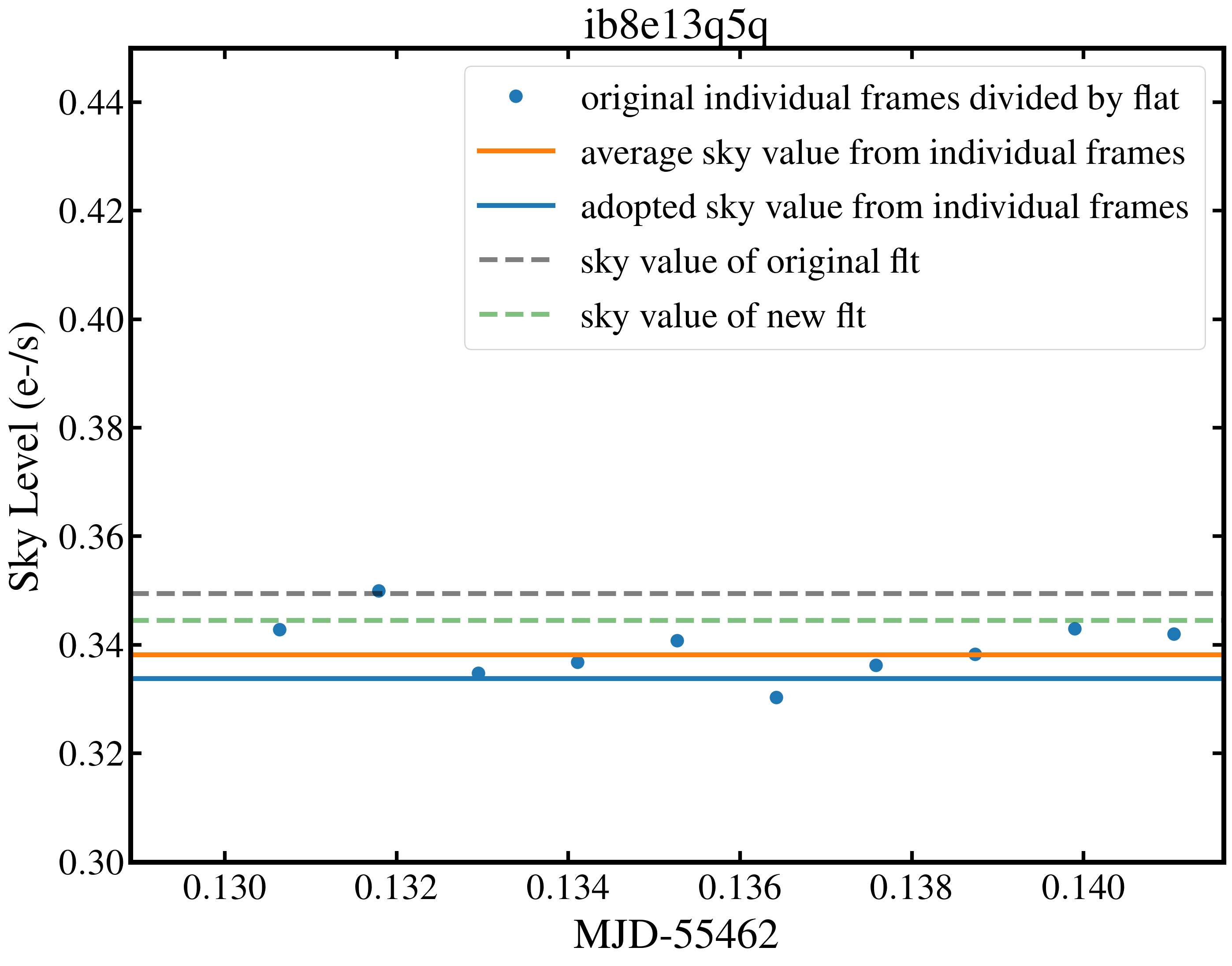
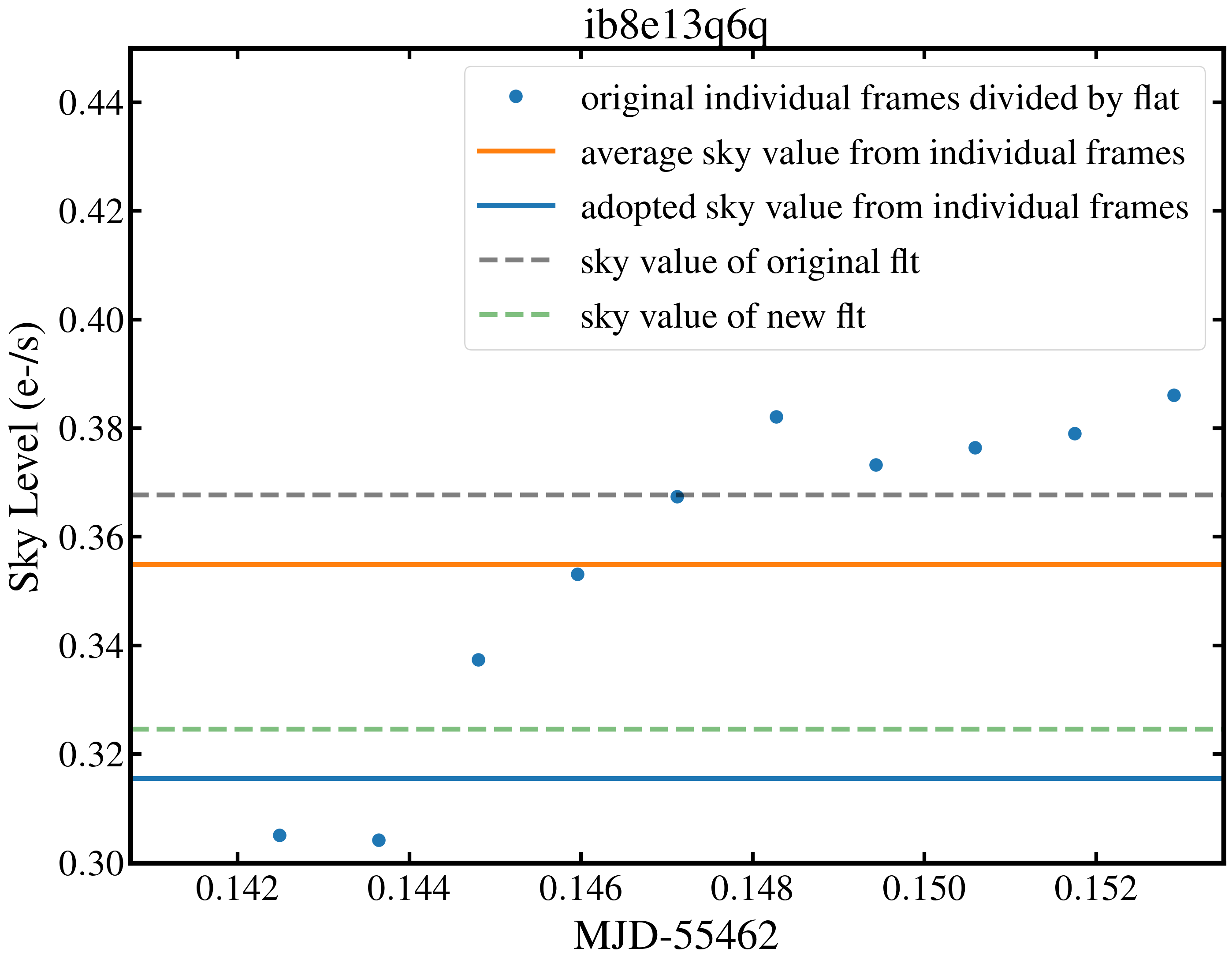
WFC3/IR — Splitting and Analyzing Exposures using Individual Ramps: The WFC3/IR detector read-outs are non-destructive, so all individual WFC3/IR exposures consist typically of 8–10 on-the-ramp sub-exposures, each of which are calibrated to facilitate correction for the numerous CR-hits and to obtain the desired exposure depth. SKYSURF measures the sky-SB in each of the 8-10 individual WFC3/IR on-the-ramp sub-exposures, which enables us to better diagnose the behavior of the sky-SB (§ 4.3) and the Thermal Dark signal ( SKYSURF-2, ) as a function of orbital phase. An example is shown in Fig. 6a–6b. This process leaves some CRs in the on-the-ramp sub-exposures, which our robust sky-SB algorithms are designed to ignore (§ 4.3 & Appendix B.1). Only the full-ramp full-exposure WFC3/IR images that have been CR-filtered are used for SKYSURF’s object counts (Appendix C).
WFC3/IR Count-Rate Non-Linearity Correction: Riess (2010) and Riess et al. (2019) discuss the changing WFC3 ZP due to its detector Count-Rate Non-Linearity (CRNL) over a very large dynamic range in flux. As a result, the WFC3/IR ZPs are slightly different for the bright calibration stars compared to faint galaxies, whose average SB is close to or below that of the Zodiacal sky-SB. In all its filters, the WFC3/IR zeropoints are subject to CRNL of about 0.0490.005 mag (or 4.50.5%) over the full range of 16 AB-mag (6.4 dex) in flux per pixel, or +0.00770.0008 mag (or +0.710.07%) over each 2.5 mag (1 dex) interval of flux per pixel. This detector CRNL is a charge trapping problem, where up to 4.5% of the faint object and faint SB-flux are lost in detector traps, and is the opposite of persistence, which is mapped and removed as described in § 4.1. WFC3/IR standard stars are measured in the total flux range of 12AB21 mag, and of course cover an area about the size of the WFC3/IR PSF, which is 0.0163 arcsec2. The sky-SB levels in the WFC3/IR broad-band filters are of order 22.6–22.3 AB-mag arcsec-2 (Table 2 of Windhorst et al., 2011) (“W11”), or 26.9 mag/PSF area. Hence, the SKYSURF sky-SB is measured at levels 6–15 mag dimmer than the pixel-signal of the standard stars used to determine the WFC3 zeropoints. We verified that the standard WFC3 pipeline calwf3 corrects all pixel SB-levels accordingly for detector CRNL. In SKYSURF, typical sky-SB levels are corrected upwards by [(6–15)/16]4.5% +(1.7–4.2)% to match the standard star flux scale, while objects with higher SB per pixel are corrected by correspondingly less. Hence, SKYSURF does not need to make further corrections for WFC3/IR detector count-rate non-linearity, but we do account for its 0.5% uncertainty in our error budget below.
WFC3 Dark Current Monitors: The WFC3/IR Dark Current (DC) has been monitored over the years (e.g., Sunnquist et al., 2017b, a, 2019). In particular, these studies show some trends in the measured WFC3/IR DC levels and structure with the four different IR detector quadrants. Also, these studies found trends of the measured WFC3/IR DC levels with telescope temperature and with HST’s of orbital phase (Sun Altitude; §4.3 & Appendix A.2.2) during the Dark Current frame observations. In O’Brien et al. (2022, in preparation), we study the WFC3/IR quadrant variations in more detail, but find them, in general, to be 0.5%, i.e., smaller than most other systematic uncertainties in measuring the sky-SB values (§ 4.2), and hence not requiring additional quadrant-dependent DC corrections. Sunnquist et al. (2017a) suggest that the rms variations in dark current level are 0.0069 e-/s, or 1% of the typical sky-SB in Fig. 1, which is incorporated into the error budget of Table 5.
The fact that the WFC3/IR Dark Current levels appear to be a function of Sun Altitude in Sunnquist et al. (2017a) prompted us to take a closer look at how much of the electronic Dark Current level is temperature-dependent — e.g., due to temperature variations in the detector A/D converters, as Sunnquist et al. (2017a) suggest — and how much additional Thermal Dark signal may be caused by HST’s temperature variations across its orbit and as a function of Sun Altitude. These aspects are addressed in § 4.3 and SKYSURF-2 as needed for the current SKYSURF results, and in more detail by Carleton et al. (2022b, in preparation) and O’Brien et al. (2022, in preparation), which will include a correction for temperature-dependent dark current variations using the Sunnquist et al. (2017a) prescription.
WFC3/IR Thermal Dark Signal: For the WFC3/IR channel, we need to distinguish between the WFC3/IR Dark Current and its Thermal Dark signal. The former is mostly an electronic current in the WFC3/IR detector that depends on the temperature of the detector and its read-out electronics, while the latter is caused by Planck black-body photons generated in HST OTA, the WFC3 housing, and the WFC3/IR detector enclosures. We need to have the best possible estimates of both to analyze the sky-SB values measured in WFC3/IR images. We will throughout refer to the WFC3/IR Thermal Dark signal as “TD” or ”TD signal”. The WFC3/IR TD signal was predicted in Table 7.11 of the WFC3 IHB (Dressel, 2012, 2016, 2021), where it is referred to as a “thermal dark current”.
The IR detector Dark Current is rather well measured out to the WFC3 shutter, which is a WFC3/IR filter slot filled with aluminum. The WFC3/IR TD signal is more uncertain and depends somewhat on the exact thermal history of each HST orbit. Predictions of the Thermal Dark signal can be made with the python package 131313https://www.stsci.edu/hst/instrumentation/reference-data-for-calibration-and-tools/synphot-throughput-tables. Tables with thermal foreground levels are incorporated into the tool, based on the observed temperatures of the HST optical and instrument components discussed in Appendix A of SKYSURF-2. In summary, our calculations of the WFC3/IR TD signal assume temperatures of the HST primary and secondary mirror of T287 K, temperatures for the WFC3 pick-off mirror and the corrective optics mirrors inside WFC3 and the IR channel of T273 K, and temperatures for the two outer enclosures and the one inner cold enclosure holding the WFC3/IR detector of T223–173 K, respectively.
To ensure that our sky-SB measurements are properly corrected for TD signal, SKYSURF-2 will conduct sky-SB estimates measurements in the three WFC3/IR broad-band filters F125W, F140W, and F160W, and correct all three for the TD signal predicted for the known ambient temperatures of the HST components. Our analysis reveals that the predicted TD signal is strongly wavelength dependent. For the F125W and F140W images, the vast majority of the TD signal comes from the WFC3/IR cold enclosure, and not from the two telescope mirrors plus the five optical-path mirrors inside WFC3, due to their much smaller solid angle as seen from the IR detector and the fact that their Planck SB is still minimal at the long-wavelength cutoff of these two bluer filters. In the F160W images, the TD contribution from the 7 mirrors in front of the WFC3/IR cold enclosure increases significantly. In SKYSURF-2, we will therefore consider a range of plausible TD values given the HST component temperatures discussed in their Appendix A. Depending on the temperature of these HST components, the predicted TD signal may vary by up to 30%. In the F160W filter, this corresponds to 2.7% of the average sky-SB, which is folded into Table 5.
4.1.5 SKYSURF Zeropoints and Zeropoint Monitors
For SKYSURF, we need to know HST’s zeropoints (ZPs) as accurately as possible from 1994–2020. Photometric stability over the years is different from photometric calibration or ZP errors. We therefore consider below in order: 1) photometric ZP definition in the context of PSF wings; 2) the actual photometric zeropoints; and 3) stability and drifts of photometric ZPs over the years. This is followed by a discussion of ZP specifics for each HST instrument used in SKYSURF.
1) Zeropoint Definition and ZP Use: For each of the HST instruments used in SKYSURF, the Data Handbooks and ISRs provide instrumental zeropoints for an object with a total flux of 1.000 /pixel/sec. These ZPs are usually offered for “compact objects” within radii 04, and for an “infinite radius aperture”. Because of the Encircled Energy (EE) curve of the spherically aberration-corrected PSF, the EE-values for point sources decrease from 91% at 04 in the F606W filter to 84% in the F125W, F140W and F160W filters due to HST’s broader PSFs at the longer wavelengths. Since the HST EE-curves approach 100% enclosed flux for 60, the “infinite radius apertures” integrate the total fluxes out to 60. For details, we refer to the ISRs by Ryan et al. (e.g., 2016), Deustua et al. (2016), and Medina et al. (2022). Most faint galaxies that SKYSURF detects to AB26.5 mag in single 500 sec SKYSURF exposures have half-light radii 02–03 (§ 4.7 & Appendix C), so their total flux is not fully captured by the “compact object” aperture ZPs at radii 04. Hence, to obtain more accurate total magnitudes for slightly resolved faint galaxies, as well as accurate sky-SB levels in the empty image areas (§ 4.2), we will always use the ZPs for “infinite radius apertures” in SKYSURF. For the current SKYSURF study, the “infinite radius apertures” ZPs provide the best absolute sky-SB values. This assumes that for a given sky-pixel and constant sky-SB, the HST PSF will leak as much flux into neighboring pixels as the neighboring pixels will leak into that pixel.
2) Photometric Zeropoints: The instrument ZPs are derived from white dwarf standard star observations, which for most filters can be done to 1% accuracy (e.g., Bohlin et al., 2020). The ACS/WFC and WFC3/UVIS and IR instrument zeropoints have been stable to 1–2% (Kalirai et al., 2010; Ryon, 2022; Dressel, 2016, 2021) with the caveats discussed below, allowing their use as absolute photometers. When comparing results from very similar broad-band filters in different instruments, small corrections for differences in central wavelength may need to be applied (see, e.g., Fig. 2a here; W11, D16; and the ICRAR zeropoint transformation tool (Koushan et al., 2021) 141414http://transformcalc.icrar.org). This is relevant when doing the objects counts over a wide dynamic range in similar filters from different instruments. Details on the filter zeropoints and aperture corrections needed for faint object fluxes and faint object counts are provided by Tompkins et al. (2022, in preparation).
3) ZP Stability and Drifts over the Years: We need to monitor and carefully account for panchromatic WFPC2, ACS/WFC, and WFC3/UVIS and IR zeropoint changes vs. time, some of which may be due to modest accumulation of contaminants onto the HST optics and in each camera over 11–18 years. This is especially true for the HST WFC3/UVIS ultraviolet filters F225W, F275W, and F336W. We discuss the relevant ZP details for each of the cameras below.
WFPC2: WFPC2’s Archival data spans over 16 years (1994–2009) with photometric zeropoints stable to within 2–3% (Holtzman et al., 1995), and 1–2% in F439W and redwards. The WFPC2 photometric zeropoints are taken from Table 10 of Holtzman et al. (1995) using their equation 9. Section 5.7 and Table 5.10 of the WFPC2 Data Handbook151515https://www.stsci.edu/instruments/wfpc2/Wfpc2_dhb/wfpc2_ch53.html#1920857 summarize the end-of-mission uncertainties in the WFPC2 calibration aspects and time-dependent zeropoints, which are summarized in Table 5. The WFCP2 ATODGAIN was read from the FITS header, and the appropriate gain ratio from Holtzman et al. (1995) was applied to correct the zeropoints for the different CCDs to AB-magnitudes.
ACS/WFC: The STScI ACS group has monitored the ACS zeropoints since its 2002 Shuttle launch on Servicing Mission 3 (SM3B). True ACS zeropoint changes are smaller than 1–2%, with drifts of order 0.1–0.2% per year. SKYSURF uses the ACS zeropoints website 161616http://acszeropoints.stsci.edu which provides this up-to-date information as a function of observing date. We use these time-dependent functions to determine the best zeropoints for the observation dates for all ACS/WFC images. From the scatter in the time-dependent zero-points in Fig. 2 of Bohlin et al. (2020), we will conservatively take this ZP-trending to be no better than 1% in accuracy, which is incorporated in the error budget of Table 5.
WFC3/UVIS: STScI has also monitored the WFC3/UVIS zeropoint
changes since its 2009 Shuttle launch on SM4 (e.g., Ryan et al., 2016; Deustua et al., 2016; Bajaj, 2019; Calamida et al., 2021). Long-term WFC3 zeropoint changes can
amount to 3% (Ryan et al., 2016) but are in part due to definition changes
in the calwf3 pipeline. True WFC3 zeropoint changes are smaller than
this, with drifts of order 0.1–0.2% per year (Calamida et al., 2021).
SKYSURF uses the WFC3/UVIS zeropoints websites 171717
https://www.stsci.edu/contents/news/wfc3-stans/wfc3-stan-issue-33-october-15,
and
https://www.stsci.edu/hst/instrumentation/wfc3/data-analysis/photometric-calibration/uvis-photometric-calibration,
which provide this up-to-date information. In particular, Calamida et al. (2021)
summarize well-sampled time-dependent zeropoint changes for most WFC3/UVIS
filters from 2009–2019. For the WFC3/UVIS UV-filters with central wavelengths
below 300 nm, the ZPs show an increase in sensitivity of +0.5%/yr for the
first two years, followed by a slowly declining sensitivity over time in
subsequent years. All filters redwards of F300X have seen a slow, nearly
linear and somewhat wavelength-dependent decline in ZP-sensitivity over time,
with well-determined slopes that typically range between –0.1%/yr to
–0.2%/yr. E.g., for the most used WFC3/UVIS F606W and F814W filters
(Table 2b), this steady decline in ZP amounts to about –1.8% and
–1.0% over 11 years, respectively. The linear fits of the
Calamida et al. (2021) zeropoint drifts have rms errors of 0.5%, and
provide the best available data on the time-dependent WFC3/UVIS zeropoints as
of 2021. To implement these slowly time-dependent ZPs as a function of
wavelength and time, we therefore downloaded the WFC3/UVIS images again in
early 2022 with calwf3 pipeline version 3.6.2 on AWS, which updated
all FITS headers with the proper time-dependent ZPs. For details of this
process, we refer to O’Brien et al. (2022, in preparation). The resulting
WFC3/UVIS ZP errors as a function of time are estimated have a 1%
accuracy, as listed in Table 5.
WFC3/IR: The WFC3/IR photometric zeropoints have roughly remained
constant to within 1.5% (rms) in the 10 years after its SM4 launch
without a noticeable time-dependent decline (Fig. 7 of Bajaj, 2019),
unlike those of WFC3/UVIS. Some of the 1.5% scatter is due to residual
persistence, which with proper dithering and drizzling can be further reduced
(Bajaj, 2019). We will therefore take the error in the WFC3/IR broad-band
ZPs to be 1.5% in Table 5. The WFC3/IR ZPs used in the
F125W, F140W, and F160W filters are 26.232, 26.450, 25.936 AB-mag,
respectively, for an object with 1.000 /pixel/sec. 181818
https://www.stsci.edu/hst/instrumentation/wfc3/data-analysis/photometric-calibration,
https://www.stsci.edu/hst/instrumentation/wfc3/data-analysis/photometric-calibration/ir-photometric-calibration,
see also http://svo2.cab.inta-csic.es/svo/theory/fps3/index.php
4.1.6 Sky-SB Error Budget Thus Far
Table 5 summarizes the error budget for WFPC2, ACS/WFC, WFC3/UVIS and WFC3/IR resulting from the considerations in § 4.1.1–4.1.5 & 4.2. For the WFC3/IR filters F125W and F140W, the total relative error is 2.7–2.8% of the average sky-SB level, while for F160W it is 3.8%, which is indicated by the brown horizontal short-dotted line in Fig. 1. The dominant sky-SB errors in Table 5 are multiplicative in nature, i.e., the global flat-field and photometric zeropoint errors. Because of the way the flat-fields and photometric zeropoints are created, these two main relative error sources are independent, so that adding them in quadrature is justified. O’Brien et al. (2022, in preparation) present a comparison between the ACS, WFC3/UVIS and WFPC2 sky-SB measurements over 26 years (e.g., 49,000 images in the F606W filter alone), enabling them to confirm our relative errors in Table 5 and — together with the WFC3/IR data — compare SKYSURF’s sky-SB values to panchromatic Zodiacal models.
The predicted WFC3/IR Thermal Dark signal error is modest in the F125W and F140W filters, but increases significantly for the F160W filter (SKYSURF-2), and therefore becomes a dominant additive error in the F160W sky-SB estimates. For this reason, the bottom two rows of Table 5 list both the lowest and the average sky-SB values plus the total errors for each in units of nW m-2 sr-1 for the WFC3/IR F125W, F140W, and F160W filters, respectively. For the darkest sky-SB values the percentage TD error is about 2 larger than the errors quoted for the average sky-SB values, increasing the total errors for the darkest sky-SB values to 2.8%, 2.9%, 6.3% in the F125W, F140W, and F160W filters, respectively. In SKYSURF-2, we will consider both the darkest and average sky-SB values in these filters, and will therefore propagate the errors of Table 5 accordingly into our results. SKYSURF-2 includes a method to avoid images with significant straylight for sky-SB estimates, which will have its own error considerations.
4.2 Optimal Object-Free Sky-SB Estimates in All Individual SKYSURF Exposures
A critical part of SKYSURF is measuring the sky-SB in between the discrete objects as accurately as possible. For this, we introduce in the next subsections different algorithms to estimate the sky-SB as well as possible in between discrete objects, which are primarily faint galaxies, Galactic stars, and CRs. To test these algorithms, we check them against simulated images with known input sky-SB values, as well as realistic distributions of galaxies, stars, and CRs. Here, we summarize how those simulations were done, how sky-SB measurements were made with different algorithms, and how these were verified. Details of these WFC3/IR image simulations and all nine SKYSURF methods used to estimate the sky-SB are given in O’Brien et al. (2022, in preparation).
4.2.1 Simulation of Images with Known Sky-SB and Realistic Cosmic Ray, Star and Galaxy Counts
Following the observed panchromatic galaxy and star counts of Windhorst et al. (2011), we generated 784 simulated WFC3/IR F125W images with known input sky-SB values, and realistic surface densities and magnitude distributions of stars and galaxies. The 784 simulated images cover the range of expected sky-SB values given the exposure time distribution in WFC3/IR F125W of Fig. 5. For about half the images we include the expected increase in sky-SB and its resulting sky-gradient in typical HST exposures towards the Earth’s limb at the end of each HST orbit, as discussed in § 4.3.
The total AB-magnitudes of both the imposed galaxy and star counts use the same WFC3/IR F125W AB-mag zeropoint of § 4.1.5 for an object with 1.000 /pixel/sec. The simulated stellar and galaxy profiles are broadened with the WFC3 PSF, while the galaxy profiles also have the ellipticity distributions superimposed as observed for faint galaxies (Odewahn et al., 1997). Finally, the images add a known sky-SB and corresponding rms sky-noise level. A variety of Zodiacal sky-SB levels are used with a range of sky-SB0.628–3.14 /pixel/sec for the range of exposure
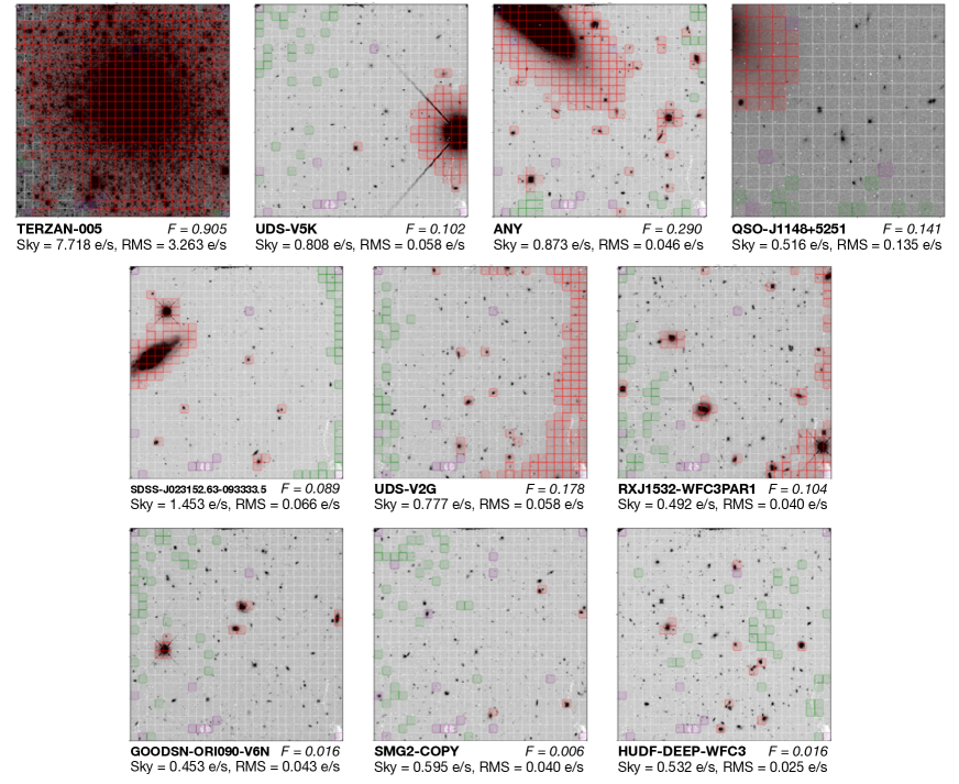
times of 50–1300 sec. Following the instrument parameters in Table 7.11 of the WFC3 IHB (Dressel, 2021), the rms noise includes the sky-noise of the imposed Zodiacal sky-level, the WFC3/IR read-noise, and Dark Current noise. Including all of these yields a typical simulated WFC3 F125W signal of 1.1 /pixel/sec, so that an average 500 sec WFC3/IR exposure has a total imposed sky-level of 556 with an rms noise of 23–24 .
In total, 784 WFC3 images were simulated by two independent teams, one following the above analytical galaxy image description that is based on well-defined statistical properties of real WFC3 images (e.g., Windhorst et al., 2011), while the other team used real WFC3 galaxy parameters as observed in CANDELS and 3DHST (van der Wel et al., 2012; Skelton et al., 2014). The latter method automatically produces the observed size distribution of § 4.7 and the observed distribution of Odewahn et al. (1997), so these parameters did not need to be imposed by the second team. These images look realistic, with the exception that real HST images show galaxies that are more irregular than the exponential disk or generalized Sersic light profiles. We validated our simulations by running the star-counts and galaxy counts on these images following the procedures described in § 4.7 and Appendix C, and concluded that the required surface densities, count slopes, and galaxy size and distributions were imposed correctly. This set of simulated WFC3/IR images with known input sky-SB levels was subsequently analyzed by different independent teams that assessed which algorithms most closely recover the known input sky-SB levels. This provides the proof of concept that SKYSURF can measure the sky-SB levels in between the discrete objects accurately, independent of their actual cause.
4.2.2 SKYSURF Algorithms to Obtain the Lowest Estimated Sky-SB in Each Exposure
SKYSURF’s specific goal is to measure the Lowest Estimated Sky-SB in each image that is not due to a statistical variation nor image defects, but is closest to the true sky-SB that SKYSURF intends to constrain. Throughout, we will refer to this Lowest Estimated Sky-SB level as “LES” or the “LES method”. In object-free areas of SKYSURF images taken during the darkest part of each HST orbit, the LES level will be as close as HST can measure to the true ZL+DGL+EBL level in that direction and time of the year. This is because all contaminating signals outside the HST instruments (e.g., Earthshine, scattered Sun and Moon light) add as a positive signal — only some of the instrument calibration errors in § 4.1 could add a dim negative signal to the images. Hence, SKYSURF needs to find this LES level in each filter in each direction of the sky, accounting also for the Earth’s Limb, Moon, and Sun Angle at that time, and flagging images that may have higher straylight values, as discussed in § 4.3.
Several different teams developed independent sky-SB estimation methods to recover the sky-SB levels imposed in the simulated images by the two separate teams in § 4.2.1. These sky-SB estimation teams had no knowledge of the actual sky-SB levels imposed by the two independent simulation teams. The only aspects they were made aware of are that the simulated images had a plausible range of sky-SB levels and exposure times (Fig. 5), surface densities of Galactic stars, galaxies with size- and ellipticity () distributions, as well as CR distributions. This process can be easily expanded to include ACS/WFC, WFC3/UVIS, or WFPC2 filters and pixel scales, to check on the wavelength dependence of the reliability of our algorithms that estimate the sky-SB using the LES method.
A total of nine methods were created to estimate LES levels in each image, each taking a different approach in identifying the best algorithm to use on real SKYSURF images (Fig. 7). These methods vary in their approach: some calculate a clipped mean, while others incorporate the ProFound (Robotham et al., 2017) package which was designed to robustly create an interpolated sky-SB map from an image. Several of the methods in Fig. 7 attempt to estimate the sky-SB by taking into account that the sky-SB might vary across a single image, i.e., indicating the presence of a sky-SB gradient (§ 4.3–4.4).
In several of the methods, SKYSURF accomplishes this by dividing each 10141014 pixel WFC3/IR image into a 2626 grid of square sub-regions or boxes that contain pixels each. Every box thus contains 1521 pixels, which is sufficient to make an estimate of its own sky-SB value accurate to 2.6% (i.e., 1/39) of the sky-rms value in that box if it contained no objects or image defects, that is, if the sky in that box were truly featureless and flat. Next, we implemented a procedure that excluded boxes based on their rms value or the number of pixels flagged in the Data Quality extension of the image, which identifies bright or faint objects or known defects in that box. The green boxes in Fig. 7 represent the lowest 5% values of the total grid of boxes that was used to estimate the Lowest Estimated Sky values in each image, i.e., those without detectable objects. We emphasize that our LES method does not look at the lowest 5% of all pixel values in each WFC3/IR image, an estimate that would certainly be biased to be well below the
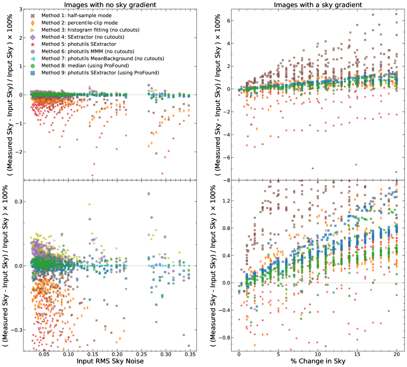
true image mode or peak. Instead, the LES method uses the lowest 5% of all boxes that were selected to not contain barely detectable faint objects, bright object outskirts, and/or image defects. We show in § 4.2.3 that using this 5% threshold of all boxes with the lowest sky-SB values most accurately recovers the known input sky-SB values from the simulations in § 4.2.1.
In SKYSURF-2, we use the best of these algorithms to estimate the LES values for all 34,400 WFC3/IR images in the F125W, F140W, and F160W images in Table 3. To check if the distribution of the green boxes in Fig. 7 showed any noticeable correlation with the GDC structure across the detector, we collapsed the green boxes from all 34,400 WFC3/IR images into one 2626 density grid. The WFC3/IR detector is on HST’s optical axis, and due to its 24∘ tilt about its x-axis, its pixels cover each a somewhat rectangular area of the sky with a 4.5% GDC variation that stretches mostly along the y-axis (see e.g., Fig. B.3 of Dressel, 2021). The average locations of the green boxes to estimate LES sky-SB values across 34,400 exposures showed no correlation with the GDC structure across the detector. Nor did they avoid the “fiducial point” in the WFC3/IR center where the GO user is recommended to place their small targets, suggesting that the average GO observer uses WFC3/IR more as a survey instrument than for individual (large) object imaging. In summary, the green boxes in Fig. 7 sample the LES values rather randomly across the detector when considering all 34,400 WFC3/IR exposures. This then justifies the sky-SB estimation in the undrizzled flat-fielded / images (§ 4.1). We will henceforth assume that the LES method estimates the lowest sky-SB in each exposure well enough to proceed.
4.2.3 Algorithm- and Scene-Dependent Reliability of Recovered Input Sky-SB
Here, we summarize the main algorithmic results and discuss the best algorithms to estimate the Lowest Estimated Sky-SB in the absence and presence of sky-SB gradients. By implementing the filtered gridding method of § 4.2.2, we are also able to indirectly detect gradients across an image. We flag and remove sub-regions that are brighter than the mean sky-SB level + the mean sky-SB rms level, then remove images where more than 30% of sub-regions are flagged as non-sky regions. A comparison of the results from these nine methods is shown in Fig. 8.
In the absence of sky-gradients, Fig. 8ac show that method 3 (based on histogram fitting; yellow triangles), and methods 8 and 9 (based on ProFound-catalogs; Robotham et al., 2017, green and blue squares) generally provide measured sky-SB levels to well within 0.2% from the known input values. In methods 8 and 9, the simulated sky-SB values are best recovered when the lowest 5% of the sky boxes’ SB-values are used as an estimator. Method 4 (based on SourceExtractor-catalogs; purple diamonds) performs worse at sky-levels with lower S/N-ratio. For methods 8 and 9, the observed–simulated difference is as small as 0.1%, as long as the WFC3/IR sky-noise is 0.24 /pixel/sec (i.e., 200 sec for its broad-band filters).
In retrospect, the resulting 0.1% accuracy of estimating the known input sky-SB values with the best algorithms makes sense. In § 4.2.2 we estimated that in the best possible case of a clean flat sky over an entire image, each of the 676 boxes of 1521 pixels could estimate its sky-value to an accuracy of 2.6% of the sky-SB in that box. For a perfectly flat sky these methods may thus recover the input sky-SB to no better than 2.6%/0.1% of the input sky-value. This is indeed about the best accuracy at which methods 8 and 9 recover the known input sky-SB values in Fig. 8ac.
Fig. 8bd show that in the presence of simulated sky-SB gradients that amount to 10–20% of the lowest sky-SB value edge-to-edge, method 8 provides measured sky-SB levels generally within 0.4% from the simulated input values when the gradients are 10%, and within 0.2% when the imposed sky-SB gradients are 5% edge-to-edge or corner-to-corner. These simulated image gradients are in excess of any gradients expected in the ZL on arcmin scales. Significant gradients with amplitudes 10% can be caused in real HST images by: a) straylight (§ 4.3); b) large artifacts; or c) large targeted objects with real astrophysical gradients (Appendix B.3). SKYSURF flags images with strong gradients or large targets or artifacts, estimates their LES values (at lower accuracy) to help diagnose these causes of straylight and straylight gradients, and where needed discards them for sky-SB analysis or object counts.
In conclusion, the histogram-fitting method 3 provides LES sky-SB values with the simplest algorithm available that is accurate to within 0.2% in SKYSURF images without gradients (Fig. 8c), but it is not proven in the presence of strong gradients. The percentile-clip method 2 works better in the presence of gradients, but has larger errors (0.3%) in images without gradients. Hence, in the first science analysis of SKYSURF-2 we will use method 3 and discard images with higher sky-SB levels and significant gradients. Methods 4, 8 and 9 are considerably more CPU intensive, since they require complete SourceExtractor- or ProFound-catalogs object catalogs to be made in advance. Overall, method 8 can provide the most accurate LES sky-SB values to within 0.1% in SKYSURF images without gradients, and to within 0.2–0.4% in images with gradients that are less than 5–10% edge-to-edge or corner-to-corner, respectively. This method will be applied to all individual SKYSURF images in O’Brien et al. (2022, in preparation), which requires the entire SKYSURF database to be processed with ProFound.
4.3 Orbital Sky-SB Dependence and Possible Sources of Straylight
We define our usable sample of SKYSURF images as a function of orbital parameters that may affect the measured image sky-SB values: Limb Angle (LA), Moon Angle (MA), Sun Angle (SA), Sun Altitude above the Earth’s Limb, the Illuminated Earth Fraction (IEF), HST’s Roll Angle (RA), and HST’s position in the Continuous Viewing Zone (CVZ). The MA and SA are defined as the angular distance between the HST pointing-direction and the center of the Moon or Sun during the exposure, respectively. Sun Altitude is defined as the Sun–Earth–HST angle, which determines the amount of Sunlight scattered off the bright Earth that can reach the HST aperture. SKYSURF does ephemeris and visual checks to identify images that got too close to: (a) the Earth’s Limb, including those taken at the bottom of the CVZ, (b) the Sun; and/or (c) the Moon. Any one of these can corrupt the sky-SB measurements, and in some cases also the SKYSURF source catalogs. Some, but not all of this information is available in the HST Engineering telemetry data, i.e., the “jit”-files that come with the raw FITS images. Where needed, we compute the parameters LA, MA, SA, and for each SKYSURF exposure. Appendix A.1 gives details on how the HST orbital parameters are calculated at any given time since its April 24, 1990 launch or its subsequent Shuttle Servicing Mission reboosts. In our current analysis, only sky-SB measurements from images with sufficient blank sky are used for the final SKYSURF analysis (§ 4.2).
A full ray-tracing of the HST straylight from first principles is beyond the scope of the SKYSURF project, and so we start with an empirical approach to trace the sky-SB measurements as a function of the orbital parameters LA, MA, SA, and , and define the ranges in these parameters where the SB-measurements are generally not significantly enhanced above the minimum in each direction, as described in Caddy & Spitler (2021). For the 249,861 ACS+WFPC2+WFC3 images, we calculate these angles and identify the angle ranges that may have resulted in enhanced straylight levels. Such exposures may still be usable for panchromatic object counts, in which case they are used in our modified drizzled pipeline (§ 4.6).
Some examples are shown in Fig. 6a–6b. Here, Fig. 6a shows the WFC3/IR F125W sky-SB values of the first half-orbit exposure at the start of an orbit, which typically uses the darker orbital part, so that the sky-SB values do not change much over the total exposure length. The blue data points show the sky-SB values of individual WFC3/IR ramp read-outs as estimated with the best algorithms in § 4.2.3. The orange line in Fig. 6a shows the exposure time-weighted average over all ramps. The default calwf3 calibration procedure of this exposure uses all these values, which results in the grey dashed line as the sky-SB value of the final file, which is biased by the ramps with the highest sky-SB. When we run this through calwf3, we find the green dashed line as the sky value of the final file, which still does not reflect the lowest possible sky-SB value for that exposure well. For WFC3/IR, we therefore adopt the average of the three ramps with the lowest sky-SB values (blue line), excluding the initial clearing readouts. We consider the blue line to be the more representative value of the Lowest Estimated Sky-SB for that exposure.
Fig. 6b shows the WFC3 F125W sky-SB at the end of a typical HST orbit, which in this case is the second half-orbit exposure observed directly after the one shown in Fig. 6a. The procedures and lines are the same as in Fig. 6a, but the differences are now much larger because in this second half-orbit WFC3/IR exposure the sky-SB values increase significantly towards the end of the orbit due to Earthshine. The resulting blue line indicates the final adopted sky-SB value compared to the calwf3 average (orange line). Over the course of this orbit, the dispersion of our reprocessed sky-SB values is smaller than the dispersion in the original sky-SB values, so our procedure results in more consistent estimates of the Lowest Estimated Sky-SB than the default calwf3 pipeline.
The GOODS North data of Giavalisco et al. (2004) were used as an initial case study to investigate the sky-SB in HST images as a function of the orbital parameters, and reduce the impact on sky-SB measurements of: (a) Earthshine due to the proximity of the Earth’s Limb; (b) the Sun Altitude above the Earth’s Limb to minimize Sunlight scattered off the bright Earth; (c) the Moon; and (d) the Sun during each exposure to minimize their straylight. The data and model predictions are shown together with their uncertainty wedges in Fig. 9. Details are given in Caddy & Spitler (2021), Caddy et al. (2022), and Appendix A.2. The ACS F850LP-filter data in GOODS-North were chosen for this study, because: (1) it is the closest filter in central wavelength to the WFC3/IR filters used to present our first SKYSURF results; (2) the high Ecliptic Latitude (57∘) of GOODS-North reduces the impact of true ZL variations on the analysis; and (3) its very large sample size. These data consist of sky-SB measurements from 1018 ACS F850LP images in the GOODS North field, which is in HST’s CVZ and covers a range of Earth Limb Angles, Sun Altitudes, Sun Angles, and Moon Angles recorded in the HST telemetry data. Only exposure times in the range of 240–1800 seconds were used for this study.
In Fig. 9a–9d, the measured sky-SB values are colored by orbital parameters that meet the SKYSURF criteria for avoiding straylight contamination. Black points are exposures that do not meet our criteria and red points are those that do. In summary, the combined boundaries in orbital parameters that yield the darkest sky-SB values as indicated by the red points are: (a) Earth’s Limb Angle LA30–40∘to avoid Earthshine; (b) Sun Altitude above the Earth
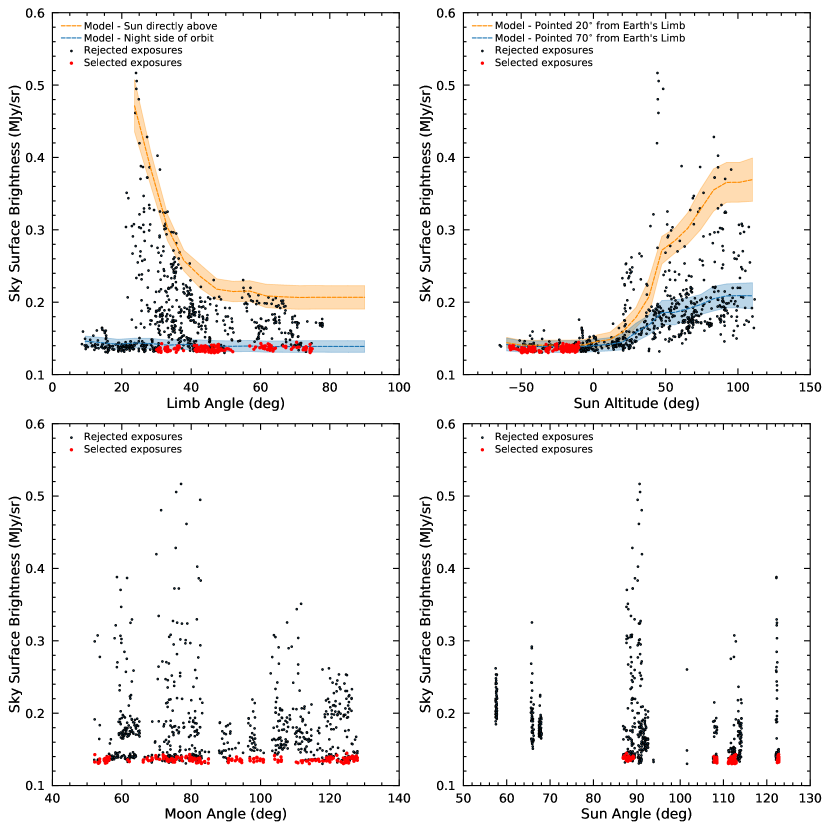
–10∘ (i.e., orbital night side) to minimize Sunlight scattered off the bright Earth; (c) Moon Angle MA50 ∘; and (d) Sun Angle SA80∘ to avoid straylight into the HST optics, respectively.
Imposing these constraints as detailed below, the standard deviation of the GOODS-N sky-SB values is reduced from 0.055 MJy/sr to 0.002 MJy/sr with an overall decrease in mean sky-SB of 0.138–0.179 MJy/sr, respectively. These selection criteria can thus minimize the impact of Earthshine, Sun Altitude, Sun Angle and Moon Angle on the HST’s sky-SB measurements. These limits are more extreme than those recommended by the HST Instrument Handbooks, and we impose them on all our panchromatic sky-SB estimates for ACS/WFC, WFC/UVIS and WFC/IR that sub-select HST’s orbital phases with the lowest straylight (O’Brien et al. 2022, in preparation). Further details on straylight resulting from the Earth’s Limb, the Sun Altitude above the bright Earth and the Sun Angle with respect to HST’s pointing direction, as well as the Moon angle are given in § A.2.
4.4 Definition and Strategy for Treatment of Sky-SB Gradients
We need to estimate and preserve the Lowest Estimated Sky-SB (LES) level in all SKYSURF images for subsequent sky-SB analysis. This is currently not the default option in AstroDrizzle 191919 https://hst-docs.stsci.edu/drizzpac/chapter-5-drizzlepac-software-package/5-2-astrodrizzle-the-new-drizzle-workhorse (Avila et al., 2015). Hence, we run AstroDrizzle on the entire SKYSURF database with the LES sky-SB preserved in each sequence of observations in a given filter that was taken in the same visit. HST exposures can have low-level gradients if they were pushed too close to the Earth’s limb, or if they were taken at too small Moon Angles or Sun Angles. An example is given in Fig. 6b. AstroDrizzle normally removes a gradient surface before drizzling, using the MDRIZSKY keyword that preserves the sky, so the subtracted sky-level or sky surface can be reinstated. We use ProFound (Robotham et al., 2017) to map low-level gradients with spline surface fits to the sky-SB in between all discrete objects detected in the SKYSURF images, preserving the spline surfaces in separate FITS files for later diagnostics. In this process, we subtract the gradient from the ProFound surface, but not the lowest reliable DC-level of the sky-SB, as that is one of the key parameters SKYSURF is measuring. Details are given by Tompkins et al. (2022, in preparation).
Images at low Galactic latitude ( 30∘), or images of large bright-object targets may have real astrophysical gradients in their sky-SB due to substantial DGL, such as Galactic star-formation regions and the outskirts of nearby galaxies. In that case, any gradient must not be removed (e.g., the top right two panels in Fig. 7). This is monitored and flagged by SKYSURF (blue column in Fig. 3), with feedback to the SKYSURF SB-measurements and drizzling database and input from the LA, MA, SA monitoring in § 4.3, to help identify which images at 30∘ may be dominated by DGL or by large bright-object targets, and not by orbital straylight.
4.5 Definition of SKYSURF Drizzle Families and Drizzle Footprints
SKYSURF drizzles all images to the same pixel scale of 0060/pixel, including the single exposures, to provide proper photometry for both sky-SB measurements and discrete object catalogs (§ 4.1). This includes the latest practices in AstroDrizzle for the identification and masking of CRs and Charge Transfer Efficiency (CTE) trails as a function of image-stack depth. Appendix B.1–B.2 describe the application of CR-removal and Charge Transfer Inefficiency trail removal over wider apertures in the calwf3 pipeline, which is applied to SKYSURF’s drizzling process.
To drizzle the SKYSURF database, we generated instrument+filter-specific on-sky footprints for all for 220,657 images with 200 sec (out of a total of 249,861 SKYSURF images), starting with their APT files. This allowed us to organize the SKYSURF database in preparation for the drizzling process, and to assess its total area (§ 3.2), which we need for accurate galaxy counts averaged over as many independent HST fields as possible (§ 2.5.2).
In total, there are 11,965 APT footprints to be drizzled in SKYSURF using a linking distance of 6 arcminutes. Each group contains all images in all available filters, whose centers are within 6 arcminutes of their nearest neighbor. The most frequently observed group has 10,761 exposure files (i.e., the HUDF), while the least frequently observed groups have only one exposure in one filter and are mostly SNAPshots. The images in each group in the same filter and instrument are then drizzled into separate mosaics. With an average of 4–5 exposures per HST orbit (Fig. 5 & Table 4), the SKYSURF database amounts to 55,000 HST orbits, or the equivalent of 15 years of HST observing time assuming an average of 3600 science orbits per year. We use all 11,965 APT footprints together with SKYSURF’s initial SB-measurements to assess which images are useful for the final set of reliable sky-SB measurements, and for the final object SourceExtractor and ProFound catalogs and all-sky object counts (Appendix C). Using the same matching algorithm, the 11,965 APT footprints contain the 4,858 independent fields of § 3.2 that are more than 1∘ away from the nearest APT footprint.
4.6 Drizzling all SKYSURF Images in AWS with Lowest Estimated Sky-SB Preserved per Image Family
The last unconventional step critical for SKYSURF is that when drizzling the images, we preserve the sky-level into all images that AstroDrizzle normally removes. This sky-level as defined in § 4.2 is carefully monitored by SKYSURF as a function of orbital phase for all multiple exposures in a given filter visit per target (§ 4.3).
In a first drizzle run, the ProFound sky-surface maps of § 4.2 are subtracted from each and its LES level is added back in. In the second drizzle run, all images in a given filter from the first run have their own LES value subtracted, followed by adding to each image the lowest LES value from that visit that went into the mosaic. Hence, each mosaic is drizzled while reinstating the lowest sky-SB value from that visit (§ 4.2–4.3). In the case of WFC3/IR — where we have more detector reads per exposure in a given visit — the average over the lowest three sky-SB values from that exposure gets reinstated to represent its sky-SB. The justification of this procedure was given in Fig. 6, Fig. 9, and § 4.3. In all cases, the subtracted ProFound sky surface maps and the reinstated constant sky-SB levels are preserved as FITS files or in the FITS header, respectively, so future users can apply them differently for other purposes. Mosaic weight-maps are also created in this process, which preserve the information on the signal-to-noise ratio in each mosaic pixel that follows from the sky-SB levels in the original images that were drizzled.
We use Amazon Web Services 202020https://aws.amazon.com/ for mass cloud computations without transferring all data files whenever possible, since the entire HST Archival database resides in AWS and is being kept up-to-date there by STScI. We use AWS to run our modified ACS and WFC3 pipelines on the HST Archival data until the end-product is as reliable as it can be. Most of the code is Python, which works well in AWS. AWS can run code or pipelines in Python, R, or C++. A few SKYSURF tasks originally developed under a FORTRAN or IRAF environment do not run on AWS and are run on the SKYSURF servers at our home institutions.
On AWS we can reprocess the HST ACS/WFC and WFC3/UVIS and IR Archive within a few months at modest costs for each iteration. We do this for the entire SKYSURF dataset. Running ProFound on all images in the entire SKYSURF database takes one full month on AWS. Central storage space of 40 TB houses the different levels of datasets for processing and distribution at ASU, plus another 40 TB to store SKYSURF’s expanded data products. In total, 80 TB of disk space at ASU and ICRAR hosts the final SKYSURF database and products. These will be made available via MAST. Details on SKYSURF’s drizzle products as they become available and their applications are given by Carter et al. (2022, in preparation).
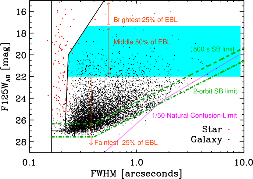
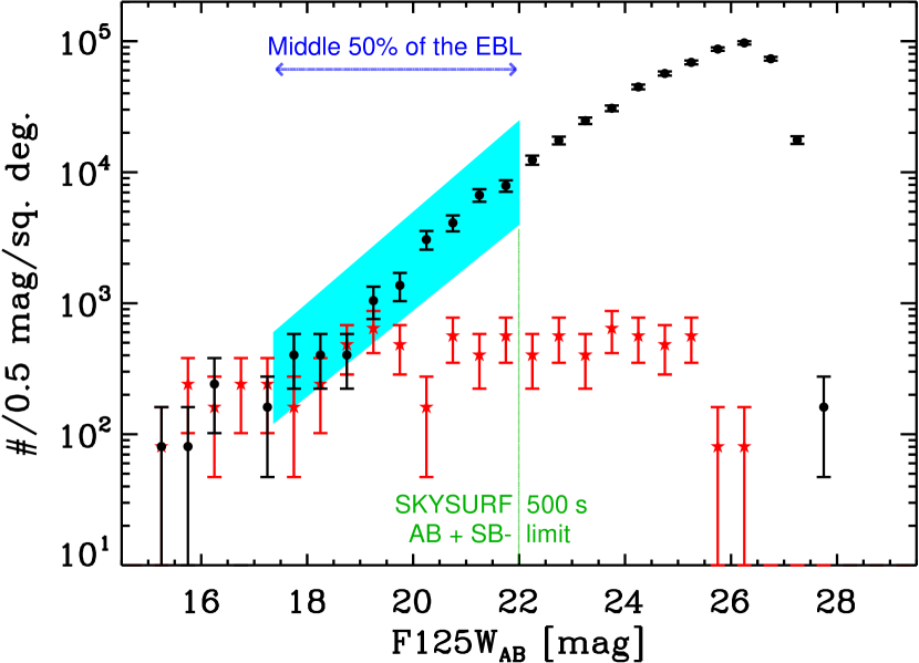
4.7 Star-Galaxy Separation, Catalog Reliability and Completeness
Our second main SKYSURF goal is to have highly reliable panchromatic HST object catalogs across the sky (Fig. 3–4). SKYSURF therefore needs to define accurate, conservative completeness limits for each object catalog. We need to determine at what magnitude bin the counts in each filter and field start to turn over from the expected power-law slope (see Windhorst et al., 2011, Driver et al., 2016b; Fig. 2 & 10–11 here). As a preliminary test, we consider images taken as part of WFC3/IR ERS program here (W11). Because of SKYSURF’s large dynamic range in flux, we can afford to cut off each individual filter catalog in each HST field at rather high significance levels. From the deeper fields, we can then determine at which flux levels each shallower catalog becomes incomplete when we do the star and galaxy counts in each field, typically at the 5–6 level for point sources. When all catalogs are combined, SKYSURF can provide accurate object counts for 16AB28 mag. Details are given in Tompkins et al. (2022, in preparation), Carleton et al. (2022b, in preparation), and Goisman et al. (2022, in preparation), including simulations to quantify incompleteness as a function of total flux, size, and SB.
Star-Galaxy Separation Method: The black slanted line in Fig. 10 illustrates SKYSURF’s star-galaxy separation method of W11, where objects were classified as stars in at least three available filters from the 10-band filter set. The average SKYSURF field will have on average only two filters available for star-galaxy separation (Table 4). Hence, SKYSURF’s star-galaxy separation process will be modified to work on fewer filters as the image drizzling, catalog production and object counting proceeds over all SKYSURF fields. The blue wedge in Fig. 10 indicates the flux range 17.4AB22 mag in F125W where galaxies contribute the central 50% of the EBL integral. The red arrows indicate the F125W flux ranges where the brightest 25%, the middle 50%, and the faintest 25% of the discrete EBL are produced, as determined from Fig. 2d (§ 2.3).
Catalog Reliability: For 17.4AB22 mag, a total of 37 objects were classified as stars (red dots) to the left of the black slanted–vertical line in Fig. 10. To the right of the black slanted line, there are 328 objects (black dots) classified as galaxies for 17.4AB22 mag, and 10 objects that were classified as stars in other filters, but are misclassified in the galaxy region in the F125W filter, although some of these could still be stars. Using such a star-galaxy separation method over this relatively bright magnitude range at HST resolution thus yields a fraction of objects misclassified as galaxies of 10/3283.0%. The ratio of classified stars-to-galaxies in this magnitude range is about 37/32811%. Because the star-to-galaxy ratio remains small at most Galactic latitudes with 30∘, SKYSURF’s galaxy samples will thus in general be more reliable (1–(10/328)97%) than its stellar samples (reliability 1–(37/47)78%).
Catalog Completeness: The two green dashed lines in Fig. 10 show the SB-limits for a typical single SKYSURF exposure of =500 sec and for a 2-orbit exposure stack, which are 25.6 and 26.8 mag arcsec-2, respectively. We use the distribution of points in Fig. 10 to estimate the catalog completeness. In the average SKYSURF exposure time of 2 orbits per filter, we expect the SKYSURF completeness limit for compact objects to be AB26–27 mag depending on the filter used, and 28 mag for the deeper HST fields. For many of the shallowest SKYSURF exposures, the completeness limit is AB25.5–26 mag (Tables 1–3 and Fig. 11).
The pink line in Fig. 10 indicates the “natural confusion” limit derived from the integrated J-band counts in Fig. 2c (represented here as a broken power law). For galaxy FWHM-sizes larger than the natural confusion limit at any given total flux, there is a 2% probability of objects overlapping due to their own finite object sizes, rather than due to the much smaller instrument PSF FWHM. Object finding algorithms may start to have issues deblending a noticeable fraction of (lower-SB) objects at sizes larger than this limit, if such objects existed (Windhorst et al., 2008, 2021). Indeed, very few objects are detected to the right of either the SB-limit and the natural confusion limit in Fig. 10. The most conservative of the two limits thus seems to be bounding the detected galaxy samples at any -value. (For deeper HST images, the natural confusion limit remains fixed, but the SB-limit improves with image depth, so the natural confusion limit thus becomes as important as the SB-limit). Together, these two limits are relevant for estimating whether a significant fraction of low-SB galaxies may have been missed at faint fluxes to explain a significant excess of diffuse EBL (Fig. 1 and SKYSURF-2, ). Further discussion is given by Windhorst et al. (2021) and Kramer et al. (2022, in preparation).
We use the two-orbit F125W data in Fig. 10 (lower green dashed lines) to estimate the incompleteness due to SB-selection in an average 500 sec SKYSURF exposure (top green dashed lines) and natural confusion (pink line). This allows us to estimate the amount of discrete, integrated, and extrapolated EBL not yet subtracted from SKYSURF’s sky-SB measurements in SKYSURF-2. For this calculation, we assume that the fraction of faint low-SB objects missing in typical 500 sec F125W exposures due to SB-selection is mostly detected in the deeper two-orbit data of W11 shown in Fig. 10. This estimate thus does not yet include any population of faint, very low-SB objects that might be missing from the deepest HST images altogether to the right of these lines in Fig. 10, which we address in SKYSURF-2. To assess the amount of possibly missing discrete, integrated, and extrapolated EBL in Fig. 2bd due to SB-selection, we estimate the 500 sec catalog incompleteness in each AB-magnitude slice from the fraction of objects known to exist in deeper HST images between the two green SB-boundaries in Fig. 10. This incompleteness amounts to 1% at AB22.0 mag and increases to 26% at AB26.0 mag. For the eight 0.5-mag slices between 22 26 mag, the incompleteness correction due to SB-selection is represented by:
| (3) |
where the quantity between square brackets is the best fit to the estimated percentage of known missing objects as a function of total AB-mag. For AB26.5 mag, sample incompleteness is not considered here, because the average 500 sec SKYSURF exposure does not reach fainter than this limit. We note that Eq. 3 would imply a SB-incompleteness of 45% at AB29 mag. The SB-incompleteness at AB29 mag is possibly that large, given the much deeper HUDF data and SB-limits plotted in Fig. 2 of Windhorst et al. (2008) and Windhorst et al. (2021). Much deeper JWST images will be needed to address the SB-incompleteness for objects with AB26–30 mag. Further considerations of SB-selection against ultra-diffuse low-SB galaxies in deep surveys are discussed in, e.g., the SMUDGES survey of Zaritsky et al. (2019), the Subaru Hyper Suprime-Cam survey of Greco et al. (2018), and future SKYSURF studies. For our average shallow SKYSURF exposures and catalogs, we adopt Eq. 3 as the minimum SB-incompleteness correction that needs to be applied for 22.0 26.5 mag to the discrete integrated EBL for objects that are known to exist in deeper HST images, but that are missing in the average 500 sec SKYSURF exposures. This is correction is applied in SKYSURF-2 to fully estimate our iEBL+eEBL values.
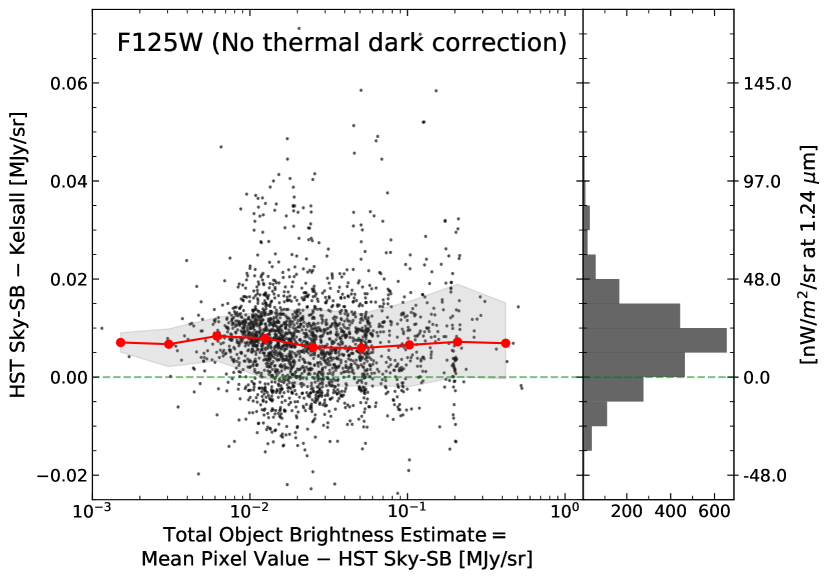
4.8 Proof-of-Concept: HST–Kelsall 1.25 µm sky-SB Difference vs. net Object SB in each Image
It is possible that stray light from discrete objects may contaminate our sky-SB measurements even with the best algorithms of § 4.2. This could be due to residual instrumental effects not recognized in § 4.1, or due to straylight from or the extended light-profiles of bright objects. While the HST cameras are in general well baffled against straylight, there are known locations just inside or outside the detector FOV where light within the telescope can scatter back onto or within the detector, thus raising the measured sky-SB levels between the discrete objects (§ 4.1.3).
To provide proof of concept of our methods in this paper, we therefore investigated whether the (sky-subtracted) total object brightness is correlated with levels of diffuse light that may be present or left in each image. We consider the total flux coming from objects in each image to be the mean pixel-value of the -image minus the LES sky-SB level as measured in § 4.2. For this test, we exclude images that may be contaminated by Earthshine or Sun Light scattered off the Earth by only considering Sun Altitudes 0∘ (§ 4.3). We also exclude images that are significantly saturated with objects, where more than 30% of the sub-regions are masked out in Fig. 7.
We perform this test on the WFC3/IR F125W images for two reasons: 1) we use WFC3/IR’s ability to flag and remove most Cosmic Rays during each on-the-ramp exposure, so that each image mean-pixel value is not skewed by bright CRs, but instead traces the sky-SB plus the total object flux in the image; 2) we can directly compare the LES sky-SB in each WFC3/IR F125W image to the Kelsall et al. (1998) COBE/DIRBE J-band Zodiacal model prediction made in the same direction and time of the year (i.e., at the same RA, Decl., t). We assume here that the HST–Kelsall sky-SB differences are a measure of diffuse light that may be present in the F125W images. Details of the applied Kelsall et al. (1998) model and the analysis of the HST-Kelsall sky-SB differences are given in SKYSURF-2.
In essence, we are testing here if the darkest WFC3/IR F125W images — where we can measure LES values close to the Zodiacal sky-SB — are largely free of residual object flux that affects the sky-SB. The results are shown in Fig. 12, where the F125W HST–Kelsall sky-SB differences are nearly constant at 0.0071 MJy/sr or 17 nW m-2 sr-1 over a factor of 100 in total object flux along the horizontal axis. Hence, Fig. 12 shows no significant trend between the HST–Kelsall sky-SB difference in each image and its total sky-subtracted object brightness. This confirms the validity of our LES method to estimate sky-SB values that are largely free of residual object flux. We will return to this residual HST–Kelsall sky-SB difference in all three WFC3/IR filters in SKYSURF-2.
In summary, it is unlikely that a residual diffuse light level is affected significantly by instrumental effects where light from discrete objects scatters back into image pixels that are part of the foreground sky-SB. This suggests that discrete objects (i.e. extended stellar or galaxy light-profiles) can be ruled out as a major source of diffuse light.
5 Discussion
In this section we briefly summarize how SKYSURF’s methods and error budget of § 4 propagate into the constraints on diffuse light that HST may see in excess of Zodiacal models. We confine ourselves to the WFC3/IR F125W filter used as an example throughout this paper. We refer to Carleton et al. (2022) [or “SKYSURF-2”] for a detailed discussion of any diffuse light signal HST may see — or limits thereto — at 1.25–1.6 µm in excess of the Kelsall et al. (1998) and Wright (1998) Zodiacal models.
The F125W filter has 6810 full on-the-ramp exposures (Table 3), of which 2337 survive the sub-selection in § 4.8. Fig. 12 suggests an average HST–Kelsall sky-SB difference of +0.00710.0138 (rms) MJy/sr, or 1733 (rms) nW m-2 sr-1. These are the values before subtraction of the WFC3/IR Thermal Dark signal and the DGL for each exposure. SKYSURF-2 discusses in detail the corrections that needs to be made to the total HST WFC3/IR diffuse sky-signal, which include subtracting the best fit TD signal from a variety of HST component temperatures, and the DGL level as estimated for each image location in the sky.
The discussion of the HST calibration, Zeropoint, sky-SB measurements and TD signal errors in § 4.1–4.2 and Table 5 suggest a 2.7% total error in our ability to estimate the F125W sky-SB. Subtraction of the DGL has its own errors, as does the comparison to any of the Zodiacal Light models. For instance, the error in the Kelsall et al. (1998) ZL model prediction is 15 nW m-2 sr-1 at 1.25 µm and 6 nW m-2 sr-1 at 2.2 µm. This amounts to 3% of their average predicted Zodiacal sky-SB. In SKYSURF-2, we thus need to add these ZL model errors in quadrature to the total sky-SB estimation error of Table 5 – appropriately interpolated for the F140W and F160W filters — before constraints can be placed on diffuse light that HST may see in excess of the Zodiacal Light models. We now have all the tools in place to do so.
Last, we return to the most recent diffuse light limits that have been placed in the visual–near-IR wavelength range, as summarized in § 2 and Fig. 1. The CIBER spectra of Matsuura et al. (2017) suggest a diffuse light component in excess of the discrete EBL of 25.612.9 nW m-2 sr-1 at 1.1 µm and 29.7 nW m-2 sr-1 at 1.6 µm compared to the Kelsall et al. (1998) model prediction as seen from 1 AU. Sano et al. (2020) reanalyze the weekly COBE/DIRBE data and suggest the existence of a total (isotropic) diffuse light component of 4510 nW m-2 sr-1 in excess of the Kelsall et al. (1998) model at 1.25 µm, which amounts to 3410 nW m-2 sr-1 after subtracting the iEBL+eEBL component of 11.20.9 nW m-2 sr-1 (Koushan et al., 2021; Carleton et al., 2022). We plot these constraints as the purple symbols in Fig. 1. Korngut et al. (2022) use spectra from 3 recent CIBER rocket flights to estimate the Equivalent Width (EW) of the Ca triplet around 8542 Å, extrapolate their result to the Kelsall et al. (1998) model prediction at 1.25 µm, and find a diffuse light component of 4619 nW m-2 sr-1 at 1.25 µm. This estimate has a larger error, but because it is based on the Ca-triplet, they suggest a residual (spheroidal) Zodiacal component that is not present in the Kelsall et al. (1998) model. Lauer et al. (2021, 2022) present 0.608 µm object counts and sky-SB measurements from New Horizons images taken at 43–51 AU (blue points with error bars in Fig. 1), where their single image obtained at 51 AU from the Sun suggests a much dimmer diffuse light signal of 8.11.9 nW m-2 sr-1 at 0.608 µm. They discuss a number of explanations for such a signal.
SKYSURF-2 will discuss the HST diffuse light constraints at 1.25–1.6 µm from SKYSURF in the context of this recent work. In O’Brien et al. (2022, in preparation) we will present the sky-SB in the broad-band ACS/WFC, WFC3/UVIS, and WFC3/IR filters of Table 1–3, and compare these results to various Zodiacal Light models at 0.2–1.7 µm. Table 1–2 shows that the full SKYSURF data set will have 49,000 images in the F606W filter alone that use all three HST cameras ACS/WFC, WFPC2, and WFC3/UVIS, allowing us to check for camera-dependent systematics. SKYSURF’s goal is then to use all these results to better constrain the Zodiacal Light models and how much diffuse light may exist at 0.2–1.7 µm as seen from Low Earth Orbit.
6 Summary and Conclusions
In this paper, we present an overview and describe the rationale, methods, and first results from the Hubble Space Telescope Archival project “SKYSURF”. The following are our main highlights and results:
(1) SKYSURF uses HST’s unique capability as an absolute photometer on timescales of decades to measure the 0.2–1.7 µm all-sky surface brightness from 249,861 WFPC2, ACS, and WFC3 exposures. Of these, 220,657 exposures have 200 sec and cover 16,822 HST FOVs that are being drizzled in on average 8 exposures per filter and 1.8 filters per target.
(2) Among these, 1400 constitute independent HST fields spread across the sky that are suitable for galaxy counts that average over Cosmic Variance, and cover an area of 10 deg2. For object detection and catalogs, our zeropoint errors are 1.5%, while for sky-SB estimates our total errors are 3–4% of the Zodiacal sky-SB.
(3) SKYSURF’s panchromatic Legacy dataset is designed to constrain the diffuse UV-near-IR sky-SB components: Zodiacal Light (inner Solar System), Kuiper Belt Objects (outer Solar System), Diffuse Galactic Light, integrated and extrapolated discrete Extragalactic Background Light (iEBL/eEBL), and the diffuse Extragalactic Background Light (dEBL).
(4) Many of SKYSURF’s goals require a non-standard re-processing of these HST images that we summarize, which include, e.g., monitoring the instrument zeropoints over 11–18 years, identifying and removing image gradients where needed, using wider object apertures to remove the outskirts of stars and galaxy images, as well as trails from CRs and Charge Transfer Inefficiency effects, and restoring into each drizzled image footprint the lowest estimated sky-level from each visit in a given image/filter combination.
(5) We present simulations of HST WFC3/IR images with known sky-values and sky-gradients, and realistic CR distributions and star plus galaxy counts. We test nine different algorithms that measure the “Lowest Estimated Sky” (LES) in each image away from the discrete objects and identified the best algorithm that recovers the inserted LES values to within 0.2% when there are no image gradients, and within 0.2–0.4% in the presence of 5–10% image gradients. Images with larger gradients are flagged for SKYSURF sky-SB analysis. Sky-SB values and image gradients are checked against Earth Limb Angle, Sun Altitude, Sun Angle, and Moon Angle, to help identify the cleanest and darkest subset of the SKYSURF images.
(6) Our WFC32/IR sky-SB estimates in the F125W, F140W, and F160W filters have errors of 2.7–3.8% of the average sky-SB, respectively. We compare our WFC3/IR F125W sky-SB estimates to the Kelsall et al. (1998) J-band Zodiacal model prediction for the same direction and time of the year. We find no significant trend between the 1.25 µm HST–Kelsall sky-SB difference for each image and its total sky-subtracted object brightness. This confirms the validity of our LES method to estimate sky-SB values that are largely free of residual object flux.
(7) Last, we will release to MAST our SKYSURF’s panchromatic legacy products with the publication of the respective sequel papers: optimized object catalogs, absolute calibrated panchromatic sky-SB data, and models of the ZL, DGL, and EBL, with pointers and documentation at the SKYSURF website at ASU (http://skysurf.asu.edu). Through this first SKYSURF paper, we invite community feedback, so we may further improve our methods as the entire SKYSURF database gets reprocessed.
References
- Alexander et al. (2005) Alexander, D. M., Bauer, F. E., Chapman, S. C., et al. 2005, ApJ, 632, 736
- Anand et al. (2022) Anand, G., Grogin, N., & Anderson, J. 2022, Revisiting ACS/WFC Sky Backgrounds, Instrument Science Report ACS 2022-1, ,
- Anderson et al. (2021) Anderson, J., Baggett, S., & Kuhn, B. 2021, Updating the WFC3/UVIS CTE model and Mitigation Strategies, Space Telescope WFC Instrument Science Report, ,
- Anderson & Bedin (2010) Anderson, J., & Bedin, L. R. 2010, PASP, 122, 1035
- Andrews et al. (2017) Andrews, S. K., Driver, S. P., Davies, L. J. M., et al. 2017, MNRAS, 464, 1569
- Andrews et al. (2018) Andrews, S. K., Driver, S. P., Davies, L. J. M., Lagos, C. d. P., & Robotham, A. S. G. 2018, MNRAS, 474, 898
- Ashby et al. (2015) Ashby, M. L. N., Willner, S. P., Fazio, G. G., et al. 2015, ApJS, 218, 33
- Astropy Collaboration et al. (2013) Astropy Collaboration, Robitaille, T. P., Tollerud, E. J., et al. 2013, A&A, 558, A33
- Astropy Collaboration et al. (2018) Astropy Collaboration, Price-Whelan, A. M., Sipőcz, B. M., et al. 2018, AJ, 156, 123
- Avila et al. (2015) Avila, R. J., Hack, W., Cara, M., et al. 2015, in Astronomical Society of the Pacific Conference Series, Vol. 495, Astronomical Data Analysis Software an Systems XXIV (ADASS XXIV), ed. A. R. Taylor & E. Rosolowsky, 281
- Bajaj (2019) Bajaj, V. 2019, WFC3/IR Photometric Repeatability, Space Telescope WFC Instrument Science Report 2019-07, ,
- Beckwith et al. (2006) Beckwith, S. V. W., Stiavelli, M., Koekemoer, A. M., et al. 2006, AJ, 132, 1729
- Bernstein (2007) Bernstein, R. A. 2007, ApJ, 666, 663
- Bernstein et al. (2002) Bernstein, R. A., Freedman, W. L., & Madore, B. F. 2002, ApJ, 571, 56
- Berta et al. (2011) Berta, S., Magnelli, B., Nordon, R., et al. 2011, A&A, 532, A49
- Bertin & Arnouts (1996) Bertin, E., & Arnouts, S. 1996, A&AS, 117, 393
- Béthermin et al. (2012) Béthermin, M., Le Floc’h, E., Ilbert, O., et al. 2012, A&A, 542, A58
- Biretta (2009) Biretta, J. 2009, WFPC2 Handbook v9.2, ,
- Biretta & Baggett (2013) Biretta, J., & Baggett, S. 2013, WFC3 Post-Flash Calibration, Space Telescope WFC Instrument Science Report, ,
- Biretta et al. (1995) Biretta, J., Ritchie, C., & Rudloff, K. 1995, A Field Guide to WFPC2 Image Anomalies, Space Telescope WFPC2 Instrument Science Report, ,
- Biteau & Williams (2015) Biteau, J., & Williams, D. A. 2015, ApJ, 812, 60
- Bohlin et al. (2020) Bohlin, R. C., Ryon, J. E., & Anderson, J. 2020, Update of the Photometric Calibration of the ACS CCD Cameras, Instrument Science Report ACS 2020-8, ,
- Borlaff et al. (2019) Borlaff, A., Trujillo, I., Román, J., et al. 2019, A&A, 621, A133
- Bradley et al. (2020) Bradley, L., Sipőcz, B., Robitaille, T., et al. 2020, astropy/photutils: 1.0.0, v.1.0.0, Zenodo, doi:10.5281/zenodo.4044744
- Brammer (2016) Brammer, G. 2016, Reprocessing WFC3/IR Exposures Affected by Time-Variable Backgrounds, Space Telescope WFC Instrument Science Report 2016-16, ,
- Brammer et al. (2014) Brammer, G., Pirzkal, N., McCullough, P., & MacKenty, J. 2014, Time-varying Excess Earth-glow Backgrounds in the WFC3/IR Channel, Space Telescope WFC Instrument Science Report 2014-03, ,
- Brammer et al. (2015) Brammer, G., Ryan, R., & Pirzkal, N. 2015, Source-dependent master sky images for the WFC3/IR grisms, Space Telescope WFC Instrument Science Report 2015-17, ,
- Budavári & Lubow (2012) Budavári, T., & Lubow, S. H. 2012, ApJ, 761, 188
- Bushouse (2008) Bushouse, H. 2008, WFC3 IR Ground P-Flats, Space Telescope WFC Instrument Science Report, ,
- Caddy & Spitler (2021) Caddy, S., & Spitler, L. 2021, in 43rd COSPAR Scientific Assembly. Held 28 January - 4 February, Vol. 43, 1534
- Caddy et al. (2022) Caddy, S. E., Spitler, L. R., & Ellis, S. C. 2022, arXiv e-prints, arXiv:2205.16002
- Calamida et al. (2021) Calamida, A., Mack, J., Medina, J., et al. 2021, New time-dependent WFC3 UVIS inverse sensitivities, Space Telescope WFC Instrument Science Report, ,
- Cambrésy et al. (2001) Cambrésy, L., Reach, W. T., Beichman, C. A., & Jarrett, T. H. 2001, ApJ, 555, 563
- Carleton et al. (2022) Carleton, T., Windhorst, R. A., O’Brien, R., et al. 2022, AJ, submitted, https://arxiv.org/abs/2205.06347
- Casertano et al. (2000) Casertano, S., de Mello, D., Dickinson, M., et al. 2000, AJ, 120, 2747
- Cohen et al. (2020) Cohen, Y., Grogin, N. A., & Bellini, A. 2020, Post-SM4 ACS/WFC L-Flats and Photometric Errors from Observations of Stellar Fields, Instrument Science Report ACS 2020-1, ,
- Cowley et al. (2019) Cowley, W. I., Lacey, C. G., Baugh, C. M., et al. 2019, MNRAS, 487, 3082
- Dauphin et al. (2022) Dauphin, F., Montes, M., Easmin, N., Bajaj, V., & McCullough, P. R. 2022, WFC3/UVIS Figure-8 Ghost Classification using Convolutional Neural Networks, Instrument Science Report WFC3 2022-3, 41 pages, ,
- Davies et al. (2015) Davies, L. J. M., Driver, S. P., Robotham, A. S. G., et al. 2015, MNRAS, 447, 1014
- Desai et al. (2019) Desai, A., Helgason, K., Ajello, M., et al. 2019, ApJ, 874, L7
- Deustua et al. (2010) Deustua, S., Long, K. S., McCullough, P., et al. 2010, in Society of Photo-Optical Instrumentation Engineers (SPIE) Conference Series, Vol. 7731, Space Telescopes and Instrumentation 2010: Optical, Infrared, and Millimeter Wave, ed. J. Oschmann, Jacobus M., M. C. Clampin, & H. A. MacEwen, 77313C
- Deustua et al. (2016) Deustua, S. E., Mack, J., Bowers, A. S., et al. 2016, UVIS 2.0 Chip-dependent Inverse Sensitivity Values, Space Telescope WFC Instrument Science Report, ,
- Dole et al. (2006) Dole, H., Lagache, G., Puget, J. L., et al. 2006, A&A, 451, 417
- Domínguez et al. (2011) Domínguez, A., Primack, J. R., Rosario, D. J., et al. 2011, MNRAS, 410, 2556
- Dressel (2012) Dressel, L. 2012, “Wide Field Camera 3 Instrument Handbook”, Version 5.0 (Baltimore: STScI)
- Dressel (2016) —. 2016, “Wide Field Camera 3 Instrument Handbook”, Version 8.0, (Baltimore: STScI), ,
- Dressel (2021) —. 2021, “Wide Field Camera 3 Instrument Handbook”, Version 13.0, (Baltimore: STScI), ,
- Driver & Robotham (2010) Driver, S. P., & Robotham, A. S. G. 2010, MNRAS, 407, 2131
- Driver et al. (1995) Driver, S. P., Windhorst, R. A., Ostrander, E. J., et al. 1995, ApJ, 449, L23
- Driver et al. (2011) Driver, S. P., Hill, D. T., Kelvin, L. S., et al. 2011, MNRAS, 413, 971
- Driver et al. (2016a) Driver, S. P., Wright, A. H., Andrews, S. K., et al. 2016a, MNRAS, 455, 3911
- Driver et al. (2016b) Driver, S. P., Andrews, S. K., Davies, L. J., et al. 2016b, ApJ, 827, 108
- Dwek & Arendt (1998) Dwek, E., & Arendt, R. G. 1998, ApJ, 508, L9
- Dwek & Krennrich (2013) Dwek, E., & Krennrich, F. 2013, Astroparticle Physics, 43, 112
- Dwek et al. (1998) Dwek, E., Arendt, R. G., Hauser, M. G., et al. 1998, ApJ, 508, 106
- Fermi-LAT Collaboration et al. (2018) Fermi-LAT Collaboration, Abdollahi, S., Ackermann, M., et al. 2018, Science, 362, 1031
- Finke et al. (2010) Finke, J. D., Razzaque, S., & Dermer, C. D. 2010, ApJ, 712, 238
- Fixsen et al. (1998) Fixsen, D. J., Dwek, E., Mather, J. C., Bennett, C. L., & Shafer, R. A. 1998, ApJ, 508, 123
- Fruchter & Hook (2002) Fruchter, A. S., & Hook, R. N. 2002, PASP, 114, 144
- Gaia Collaboration et al. (2021) Gaia Collaboration, Brown, A. G. A., Vallenari, A., et al. 2021, A&A, 649, A1
- Giavalisco et al. (2004) Giavalisco, M., Ferguson, H. C., Koekemoer, A. M., et al. 2004, ApJ, 600, L93
- Gonzaga & Biretta (2010) Gonzaga, S., & Biretta, J. 2010, WFPC2 Handbook v5.0, ,
- Gosmeyer (2017) Gosmeyer, C. M. 2017, WFC3 Anomalies Flagged by the Quicklook Team, Instrument Science Report WFC3 2017-22, 81 pages, ,
- Greco et al. (2018) Greco, J. P., Greene, J. E., Strauss, M. A., et al. 2018, ApJ, 857, 104
- Green et al. (2019) Green, G. M., Schlafly, E., Zucker, C., Speagle, J. S., & Finkbeiner, D. 2019, ApJ, 887, 93
- Grogin et al. (2011) Grogin, N. A., Kocevski, D. D., Faber, S. M., et al. 2011, ApJS, 197, 35
- H. E. S. S. Collaboration et al. (2013) H. E. S. S. Collaboration, Abramowski, A., Acero, F., et al. 2013, A&A, 550, A4
- Hathi et al. (2010) Hathi, N. P., Ryan, R. E., J., Cohen, S. H., et al. 2010, ApJ, 720, 1708
- Hauser & Dwek (2001) Hauser, M. G., & Dwek, E. 2001, ARA&A, 39, 249
- Hauser et al. (1998) Hauser, M. G., Arendt, R. G., Kelsall, T., et al. 1998, ApJ, 508, 25
- HAWC Collaboration (2022) HAWC Collaboration. 2022, arXiv e-prints, arXiv:2204.12166
- Holtzman et al. (1995) Holtzman, J. A., Burrows, C. J., Casertano, S., et al. 1995, PASP, 107, 1065
- Hopkins et al. (2013) Hopkins, A. M., Driver, S. P., Brough, S., et al. 2013, MNRAS, 430, 2047
- Hopwood et al. (2010) Hopwood, R., Serjeant, S., Negrello, M., et al. 2010, ApJ, 716, L45
- Ilbert et al. (2005) Ilbert, O., Tresse, L., Zucca, E., et al. 2005, A&A, 439, 863
- Jauzac et al. (2011) Jauzac, M., Dole, H., Le Floc’h, E., et al. 2011, A&A, 525, A52
- Kalirai et al. (2010) Kalirai, J. S., Baggett, S., Borders, T., & Rajan, A. 2010, The Photometric Performance of WFC3/UVIS: Temporal Stability Through Year 1, Space Telescope WFC Instrument Science Report 2010-14, ,
- Kashlinsky (2005) Kashlinsky, A. 2005, Phys. Rep., 409, 361
- Kashlinsky & Odenwald (2000) Kashlinsky, A., & Odenwald, S. 2000, ApJ, 528, 74
- Kawara et al. (2017) Kawara, K., Matsuoka, Y., Sano, K., et al. 2017, PASJ, 69, 31
- Keenan et al. (2010) Keenan, R. C., Barger, A. J., Cowie, L. L., & Wang, W. H. 2010, ApJ, 723, 40
- Kelsall et al. (1998) Kelsall, T., Weiland, J. L., Franz, B. A., et al. 1998, ApJ, 508, 44
- Khaire & Srianand (2015) Khaire, V., & Srianand, R. 2015, ApJ, 805, 33
- Koekemoer et al. (2011) Koekemoer, A. M., Faber, S. M., Ferguson, H. C., et al. 2011, ApJS, 197, 36
- Koekemoer et al. (2013) Koekemoer, A. M., Ellis, R. S., McLure, R. J., et al. 2013, ApJS, 209, 3
- Korngut et al. (2022) Korngut, P. M., Kim, M. G., Arai, T., et al. 2022, ApJ, 926, 133
- Koushan et al. (2021) Koushan, S., Driver, S. P., Bellstedt, S., et al. 2021, MNRAS, 503, 2033
- Lagache et al. (1999) Lagache, G., Abergel, A., Boulanger, F., Désert, F. X., & Puget, J. L. 1999, A&A, 344, 322
- Lagache et al. (2005) Lagache, G., Puget, J.-L., & Dole, H. 2005, ARA&A, 43, 727
- Landsman (1993) Landsman, W. B. 1993, in Astronomical Society of the Pacific Conference Series, Vol. 52, Astronomical Data Analysis Software and Systems II, ed. R. J. Hanisch, R. J. V. Brissenden, & J. Barnes, 246
- Lauer (1999) Lauer, T. R. 1999, PASP, 111, 227
- Lauer et al. (2021) Lauer, T. R., Postman, M., Weaver, H. A., et al. 2021, ApJ, 906, 77
- Lauer et al. (2022) Lauer, T. R., Postman, M., Spencer, J. R., et al. 2022, ApJ, 927, L8
- Leinert et al. (1998) Leinert, C., Bowyer, S., Haikala, L. K., et al. 1998, A&AS, 127, 1
- Liske et al. (2015) Liske, J., Baldry, I. K., Driver, S. P., et al. 2015, MNRAS, 452, 2087
- Long et al. (2010) Long, K. S., Baggett, S., Deustua, S., & Riess, A. 2010, WFC3/IR Persistence as Measured in Cycle 17 using Tungsten Lamp Exposures, Space Telescope WFC Instrument Science Report 2010-17, ,
- Long et al. (2012) Long, K. S., Baggett, S. M., MacKenty, J. W., & Riess, A. G. 2012, in Society of Photo-Optical Instrumentation Engineers (SPIE) Conference Series, Vol. 8442, Space Telescopes and Instrumentation 2012: Optical, Infrared, and Millimeter Wave, ed. M. C. Clampin, G. G. Fazio, H. A. MacEwen, & J. Oschmann, Jacobus M., 84421W
- Lorentz et al. (2015) Lorentz, M., Brun, P., & Sanchez, D. 2015, in International Cosmic Ray Conference, Vol. 34, 34th International Cosmic Ray Conference (ICRC2015), 777
- Mack et al. (2021) Mack, J., Olszewksi, H., & Pirzkal, N. 2021, WFC3/IR Filter-Dependent Sky Flats, Space Telescope WFC Instrument Science Report, ,
- Mack et al. (2015) Mack, J., Rajan, A., & Bowers, A. 2015, Spatial Accuracy of the UVIS Flat Fields, Instrument Science Report WFC3 2015-18, 23 pages, ,
- Madau & Dickinson (2014) Madau, P., & Dickinson, M. 2014, ARA&A, 52, 415
- Madau & Pozzetti (2000) Madau, P., & Pozzetti, L. 2000, MNRAS, 312, L9
- Magnelli et al. (2013) Magnelli, B., Popesso, P., Berta, S., et al. 2013, A&A, 553, A132
- Matsumoto et al. (2005) Matsumoto, T., Matsuura, S., Murakami, H., et al. 2005, ApJ, 626, 31
- Matsumoto et al. (2011) Matsumoto, T., Seo, H. J., Jeong, W. S., et al. 2011, ApJ, 742, 124
- Matsuura et al. (2011) Matsuura, S., Shirahata, M., Kawada, M., et al. 2011, ApJ, 737, 2
- Matsuura et al. (2017) Matsuura, S., Arai, T., Bock, J. J., et al. 2017, ApJ, 839, 7
- Mattila (2006) Mattila, K. 2006, MNRAS, 372, 1253
- Mattila et al. (2017) Mattila, K., Väisänen, P., Lehtinen, K., von Appen-Schnur, G., & Leinert, C. 2017, MNRAS, 470, 2152
- McMaster & Whitmore (2002) McMaster, M., & Whitmore, B. 2002, Updated Contamination Rates for WFPC2 UV Filters, Space Telescope WFPC2 Instrument Science Report, ,
- McVittie & Wyatt (1959) McVittie, G. C., & Wyatt, S. P. 1959, ApJ, 130, 1
- Medina et al. (2022) Medina, J., Mack, J., & Calamida, A. 2022, WFC3/UVIS Encircled Energy, Instrument Science Report WFC3 2022-2, 23 pages, ,
- Miles et al. (2020) Miles, N. D., Deustua, S., & Tancredi, G. 2020, HSTCosmicrays: Analyzing cosmic rays in HST calibration data, , , ascl:2011.021
- Miles et al. (2018) Miles, N. D., Lim, P.-L., Bellini, A., & Grogin, N. A. 2018, Updates to the CALACS Cosmic Ray Rejection Routine: ACSREJ, Instrument Science Report ACS 2018-05, ,
- Moster et al. (2011) Moster, B. P., Somerville, R. S., Newman, J. A., & Rix, H.-W. 2011, ApJ, 731, 113
- Odewahn et al. (1997) Odewahn, S. C., Burstein, D., & Windhorst, R. A. 1997, AJ, 114, 2219
- Odewahn et al. (1996) Odewahn, S. C., Windhorst, R. A., Driver, S. P., & Keel, W. C. 1996, ApJ, 472, L13
- Oke & Gunn (1983) Oke, J. B., & Gunn, J. E. 1983, ApJ, 266, 713
- Olszewski & Mack (2021) Olszewski, H., & Mack, J. 2021, WFC3/IR Blob Flats, Space Telescope WFC Instrument Science Report, ,
- Partridge & Peebles (1967a) Partridge, R. B., & Peebles, P. J. E. 1967a, ApJ, 147, 868
- Partridge & Peebles (1967b) —. 1967b, ApJ, 148, 377
- Pirzkal (2014) Pirzkal, N. 2014, ISR WFC3 2014-11 (STScI), Space Telescope WFC3 Instrument Science Report, ,
- Pirzkal et al. (2011) Pirzkal, N., Mack, J., Dahlen, T., & Sabbi, E. 2011, Sky Flats: Generating Improved WFC3 IR Flat-fields, Space Telescope WFC Instrument Science Report, ,
- Pirzkal & Ryan (2020) Pirzkal, N., & Ryan, R. 2020, The Dispersed infrared background in WFC3 G102 and G141 observations, Space Telescope WFC Instrument Science Report, ,
- Pirzkal et al. (2010) Pirzkal, N., Viana, A., & Rajan, A. 2010, The WFC3 IR ’Blobs”, Space Telescope WFC Instrument Science Report, ,
- Pirzkal et al. (2009) Pirzkal, N., Burgasser, A. J., Malhotra, S., et al. 2009, ApJ, 695, 1591
- Planck Collaboration et al. (2016) Planck Collaboration, Ade, P. A. R., Aghanim, N., et al. 2016, A&A, 594, A13
- Puget et al. (1996) Puget, J. L., Abergel, A., Bernard, J. P., et al. 1996, A&A, 308, L5
- Rafelski et al. (2015) Rafelski, M., Teplitz, H. I., Gardner, J. P., et al. 2015, AJ, 150, 31
- Rajan & Baggett (2010) Rajan, A., & Baggett, S. 2010, WFC3 SMOV Proposal 11432: UVIS Internal Flats, Space Telescope WFC Instrument Science Report, ,
- Riess (2010) Riess, A. G. 2010, First On-orbit Measurements of the WFC3-IR Count-rate Non-Linearity, Space Telescope WFC Instrument Science Report, ,
- Riess et al. (2019) Riess, A. G., Narayan, G., & Calamida, A. 2019, Calibration of the WFC3-IR Count-rate Nonlinearity, Sub-percent Accuracy for a Factor of a Million in Flux, Space Telescope WFC Instrument Science Report, ,
- Robotham et al. (2018) Robotham, A. S. G., Davies, L. J. M., Driver, S. P., et al. 2018, MNRAS, 476, 3137
- Robotham et al. (2017) Robotham, A. S. G., Taranu, D. S., Tobar, R., Moffett, A., & Driver, S. P. 2017, MNRAS, 466, 1513
- Ryan et al. (2016) Ryan, R. E., J., Deustua, S., Sosey, M., et al. 2016, The Updated Calibration Pipeline for WFC3/UVIS: a Reference Guide to calwf3 (version 3.3), Space Telescope WFC Instrument Science Report 2016-01, ,
- Ryan et al. (2017) Ryan, Russell E., J., Thorman, P. A., Schmidt, S. J., et al. 2017, ApJ, 847, 53
- Ryan et al. (2011) Ryan, R. E., Thorman, P. A., Yan, H., et al. 2011, ApJ, 739, 83
- Ryon (2022) Ryon, J. E. 2022, “ACS Instrument Handbook”, Version 21.0, (Baltimore: STScI), ,
- Saldana-Lopez et al. (2021) Saldana-Lopez, A., Domínguez, A., Pérez-González, P. G., et al. 2021, MNRAS, 507, 5144
- Sano et al. (2020) Sano, K., Matsuura, S., Yomo, K., & Takahashi, A. 2020, ApJ, 901, 112
- Schlafly & Finkbeiner (2011) Schlafly, E. F., & Finkbeiner, D. P. 2011, ApJ, 737, 103
- Skelton et al. (2014) Skelton, R. E., Whitaker, K. E., Momcheva, I. G., et al. 2014, ApJS, 214, 24
- Smith et al. (2018) Smith, B. M., Windhorst, R. A., Jansen, R. A., et al. 2018, ApJ, 853, 191
- Smith et al. (2020) Smith, B. M., Windhorst, R. A., Cohen, S. H., et al. 2020, ApJ, 897, 41
- Smith et al. (1993) Smith, R. W., Hanle, P. A., Kargon, R. H., & Tatarewicz, J. N. 1993, The Space Telescope. A study of NASA, science, technology, and politics.
- Somerville et al. (2004) Somerville, R. S., Lee, K., Ferguson, H. C., et al. 2004, ApJ, 600, L171
- Suchkov & Baggett (2012) Suchkov, A., & Baggett, S. 2012, WFC3/UVIS Crosstalk and Crosstalk Correction, Space Telescope WFC Instrument Science Report 2012-02, ,
- Sunnquist et al. (2017a) Sunnquist, B., Baggett, S., & Long, K. S. 2017a, A Predictive WFC3/IR Dark Current Model, Space Telescope WFC Instrument Science Report 2017-24, ,
- Sunnquist et al. (2017b) —. 2017b, An Exploration of WFC3/IR Dark Current Variation, Space Telescope WFC Instrument Science Report 2017-04, ,
- Sunnquist et al. (2019) Sunnquist, B., Mckay, M., & Baggett, S. 2019, Time-dependent WFC3/IR Superdarks, Space Telescope WFC Instrument Science Report 2019-04, ,
- Teplitz et al. (2013) Teplitz, H. I., Rafelski, M., Kurczynski, P., et al. 2013, AJ, 146, 159
- Totani et al. (2001) Totani, T., Yoshii, Y., Iwamuro, F., Maihara, T., & Motohara, K. 2001, ApJ, 550, L137
- Trenti & Stiavelli (2008) Trenti, M., & Stiavelli, M. 2008, ApJ, 676, 767
- Tsumura et al. (2013) Tsumura, K., Matsumoto, T., Matsuura, S., Sakon, I., & Wada, T. 2013, PASJ, 65, 121
- Vaiana & Baggett (2010) Vaiana, A. C., & Baggett, S. 2010, WFC3 TV3 Testing: IR Crosstalk, Space Telescope WFC Instrument Science Report 2010-02, ,
- van der Wel et al. (2012) van der Wel, A., Bell, E. F., Häussler, B., et al. 2012, ApJS, 203, 24
- van Dokkum (2001) van Dokkum, P. G. 2001, PASP, 113, 1420
- Whitmore et al. (2016) Whitmore, B. C., Allam, S. S., Budavári, T., et al. 2016, AJ, 151, 134
- Wielicki et al. (1996) Wielicki, B. A., Barkstrom, B. R., Harrison, E. F., et al. 1996, Bulletin of the American Meteorological Society, 77, 853
- Williams et al. (1996) Williams, R. E., Blacker, B., Dickinson, M., et al. 1996, AJ, 112, 1335
- Windhorst et al. (1992) Windhorst, R., Mathis, D. F., & Keel, W. C. 1992, ApJ, 400, L1
- Windhorst et al. (1994a) Windhorst, R. A., Franklin, B. E., & Neuschaefer, L. W. 1994a, PASP, 106, 798
- Windhorst et al. (2008) Windhorst, R. A., Hathi, N. P., Cohen, S. H., et al. 2008, Advances in Space Research, 41, 1965
- Windhorst et al. (1998) Windhorst, R. A., Keel, W. C., & Pascarelle, S. M. 1998, ApJ, 494, L27
- Windhorst et al. (1994b) Windhorst, R. A., Schmidtke, P. C., Pascarelle, S. M., et al. 1994b, AJ, 107, 930
- Windhorst et al. (2011) Windhorst, R. A., Cohen, S. H., Hathi, N. P., et al. 2011, ApJS, 193, 27
- Windhorst et al. (2018) Windhorst, R. A., Timmes, F. X., Wyithe, J. S. B., et al. 2018, ApJS, 234, 41
- Windhorst et al. (2021) Windhorst, R. A., Carleton, T., Cohen, S. H., et al. 2021, arXiv e-prints, 1
- Wright (1998) Wright, E. L. 1998, ApJ, 496, 1
- Xu et al. (2005) Xu, C. K., Donas, J., Arnouts, S., et al. 2005, ApJ, 619, L11
- York et al. (2000) York, D. G., Adelman, J., Anderson, John E., J., et al. 2000, AJ, 120, 1579
- Zaritsky et al. (2019) Zaritsky, D., Donnerstein, R., Dey, A., et al. 2019, ApJS, 240, 1
- Zemcov et al. (2017) Zemcov, M., Immel, P., Nguyen, C., et al. 2017, Nature Communications, 8, 15003
Appendix A HST Orbital Parameters and Orbital Straylight
In Appendix A.1–A.2, we give a summary of the calculation of HST’s orbital parameters, as well as of straylight from the Earth, Sun and Moon across HST’s orbital phases. In Appendix A of SKYSURF-2 we also give summary of HST’s known thermal behavior as documented in its telemetry data.
A.1 Calculation of HST Orbital Parameters
The Earth’s Limb Angle (LA) is recorded in the jit-files every few seconds during an exposure. SKYSURF retrieves this information for all ACS/WFC3, WFPC2, and WFC3/UVIS and IR images. The run of LA’s across a WFC3/IR exposure has to be recomputed using the post-observing ephemerides of HST. We developed code to generalize this, and obtain a good match to these jit-values compared to ephemerides. The LA-predicting software 212121https://www.qsl.net/kd2bd/predict.html (IDL) and https://github.com/npirzkal/EarthPlot (Python) calculates the exact past HST orbital parameters (in 6-dimensional space + velocity coordinates: , , ; , , ) in the geocentric system for any time in the past, which can be retrieved from the NORAD database 222222http://www.celestrak.com/NORAD/archives/request.php, where HST is satellite number 20580. The NORAD satellite archive returns a file that needs to be split into individual HST orbital files, done with IDL routine split_hstorbits.pro. The results are saved in a .predict folder, and the LA is calculated with limbangle.pro, which updates the predict files for each orbit. Together with the past HST ephemerides, these calculations also include the Illuminated Earth Fraction (IEF) as a parameter that can affect the amount straylight in the individual SKYSURF images (§ 4.3). Because of Earth-limb straylight possibly reflecting differently off the HST OTA cover at different off-nominal roll angles (RAs), this code can also help trace the sky-SB as a function of off-nominal RA and IEF as needed (Caddy et al., 2022).
It should be noted that COBE’s orbit is at an average Low Earth Orbit (LEO) altitude of 885 km, while HST is at an average orbital altitude of 539 km. The HST orbital altitude was somewhat higher early in the mission, and it has slightly decayed during the 1991, 2002, and 2013 Solar maxima, but some altitude was recovered due to reboosts from several of its five Shuttle Servicing Missions. Given the very low atmospheric emission at 539–885 km altitude in directions well away from the Earth (other than Geocoronal lines such as Ly at 1216 Å and He II at 1.083 µm), we will assume that the orbital altitude difference between the HST and COBE is not the main source of any differences in 1.25–1.6 µm sky-SB measurements between the two missions discussed in SKYSURF-2. This is supported by MSISE-90 Upper Atmospheric models of the Earth 232323http://www.braeunig.us/space/atmos.htm, which lists that the mean atmospheric pressure is 2.2710-7 Pa at 540 km, while it is 1.0410-8 Pa at 885 km.
A.2 HST Orbital Straylight
This section gives further details on straylight due to proximity to the Earth’s Limb, the Sun Altitude above the bright Earth and the Sun Angle with respect to HST’s pointing direction, as well as due to the Moon angle.
A.2.1 Earth’s Limb Angle
Eliminating levels of scattered Earthshine contamination in exposures used in deriving sky-SB levels is paramount to the core science goals of SKYSURF. All orbital parameters that may impact the Earthshine intensity in exposures must be considered. SKYSURF thus needs to identify all exposures impacted by Earthshine or scattered light, and flag those. To ensure that Earthshine is limited to a minimum, one would need to select only those fields that were taken in orbital dark time, which meet the SHADOW or LOW-SKY Special Requirements. STScI developed these options for this purpose early in the HST mission, as can be seen in the current version of APT. However, not every HST observer who asked for orbital SHADOW or LOW-SKY time in their APT file did, in fact, receive it, nor did every observer who received orbital SHADOW or LOW-SKY time ask for it.
We flag all individual images that came too close to the Earth’s limb (LA40–60∘), irrespective of whether the observer asked for orbital dark time or not. For WFC3/IR, we do this also using individual time-samples within an exposure as in Fig. 9a–9b. Since the orbital dark time does not generally exceed 1800 sec per HST orbit, the simplest approach is to sub-select only those exposures in the range 200–1800 sec. Exposures longer than 2100 sec often run into elevated sky due to proximity to the Earth’s limb. An example is given by the green 0.23 and 1.6 µm-points in Fig. 1, which are for these reasons higher than the expected Zodiacal SB-values that are normalized to the Solar spectrum, as discussed in Windhorst et al. (2018).
Fig. 9a shows the sky-SB as a function of Earth’s Limb Angle. The orange line and model uncertainty wedge of Caddy et al. (2022) show the elevated sky-SB due to Earthshine for Sun Altitude 90∘ on the orbital day side with the SA fixed at 90∘. The model cuts off at LA20∘ due to HST scheduling constraints. A strong exponential increase is seen for fields taken on the day side of the orbit with LA40–45∘, but even fields with LA70–80∘ on the day side have an elevated sky-SB. The blue line plus uncertainty error wedge indicates the Caddy et al. (2022) model on the night side for –10∘, and shows a marked decrease in sky-SB. The model extends to LA10∘ due to scheduling constraints on the night side. Deviation from an otherwise flat relation is seen for fields with LA20∘ on the night side. Exposures that have 10LA20∘ and also 0∘ have reduced sky-SB, but with somewhat increased scatter due to the shallow Limb Angle.
In summary, Earthshine increases strongly as a function of Limb Angle. This is also visible in FIGS WFC3/IR grism data (e.g., Pirzkal, 2014; Brammer et al., 2015; Brammer, 2016). The 1.083 µm Geocoronal He II line can be quite bright and contaminate WFC3 near-IR images in the F105W and F110W filters and the G102 grism (Brammer et al., 2014; Pirzkal & Ryan, 2020), so F105W and F110W images with increased sky-SB levels are also flagged for this reason. SKYSURF-2 shows that the HST WFC3/IR F125W and COBE/DIRBE J-band filters exclude the 1.083 µm Geocoronal He II line, if it were present at low Limb Angles. The WFC3/IR filters F125W, F140W, and F160W used for our first SKYSURF results in Carleton et al. (2022) are thus free of the brightest known Geocoronal emission lines.
A.2.2 Sun Altitude and Sun Angle
In addition to the Earth’s Limb Angle, the Sun Altitude above the Earth’s Limb, the Sun Angle, and the Moon Angle [both measured from HST’s pointing direction] over the duration of an exposure must be identified and constrained to minimize Sunlight scattered off the bright Earth, or off the IPD cloud at angles too close to the Sun. The results of this analysis are shown in Fig. 9c–9d.
Sun Altitude (): The Sun Altitude limit is found to be the most influential parameter in reducing Earthshine contamination, followed by the Limb Angle limit. For SKYSURF data the Sun Altitude limit is chosen to be all exposures with –10∘. Earthshine directly below the location of HST can be assessed independently from surface flux measurements at 0.3–5 µm wavelengths by the CERES (Clouds and the Earth’s Radiant Energy System) satellite over the duration of the same Low-Earth orbit (Wielicki et al., 1996). This enables us to monitor Earthshine levels in real time on the day side of an HST orbit underneath the telescope, where the intensity of Earthshine cannot be accurately predicted due to the complex nature of the weather systems below (Caddy & Spitler, 2021). This work suggests that higher Earthshine levels are found to potentially contaminate HST fields with Sun Altitudes values –10∘ or more on the day side of an orbit. Fig. 9b shows the sky-SB as a function of Sun Altitude . The orange and blue lines plus model uncertainty wedges of Caddy et al. (2022) show that lower LA’s result in steeper relationships for Sun Altitudes 10–20∘ due to the increased Sunlight scattered off the bright Earth. In this CVZ dataset — and in many others — the Sun Altitude can be 90∘ and in GOODS-N up to 110∘ (Fig. 9b), or 20∘ towards HST’s aperture as seen from HST’s “local Zenith”. Such angles almost certainly increase Solar straylight off the bright Earth, depending on HST’s roll angle and how its aperture door faces the illuminated Earth. For –10∘, the sky-SB is lowest and remains approximately constant. As a result, no day-side exposures are used in the final SKYSURF sky-SB analysis. This constraint considerably reduces the amount of usable data in the archive but is necessary to prevent significant Earthshine contamination.
Sun Angle: Fig. 9d shows that the minimum HST sky-SB levels increase for Sun Angles80∘, including on the night side of an orbit, in part due to an increase in ZL intensity closer to the Sun. Standard HST scheduling constraints of SA50∘ are observed. HST observations are often scheduled at or near SA90∘ or “nominal roll” angle to ensure optimal illumination of the solar array. Sun Angles are therefore clustered corresponding to the date of the exposures. The large scatter in the sky-SB levels around each Sun Angle is primarily due to the variation in Sun Altitude and Limb Angle for each exposure. Due to the degeneracy between elevated ZL and scattered Sunlight inside the HST telescope tube, it is not possible to identify the dominant cause of elevated sky-SB for Sun Angles SA80∘. As a result, we will avoid Sun Angles SA80∘ for our final SKYSURF sample.
A.2.3 Moon Angle
Fig. 9c shows the sky-SB as a function of Moon Angle. For the Moon, the HST avoidance angle is typically MA50∘. At MA50∘, the Moon Angle is not the major driver of increased sky-SB.
Appendix B Specific SKYSURF Requirements for Image Drizzling and Image Filtering
In this section, we discuss the application of wider-apertures for the removal of trails from cosmic rays (CRs) and Charge Transfer Inefficiency effects during drizzling. We also give details on SKYSURF’s methods to identify and remove HST images with large artifacts, and HST images with large targets that overfill the FOV. In all cases, fields that are discarded during the flagging process in Appendix B.3 must have a known reason for their omission to avoid biasing the remaining sample with galaxy counts in Appendix C that are too low or too high. Further details are given in Tompkins et al. (2022, in preparation).
B.1 Application of Wider-Aperture Cosmic Ray Removal during Drizzling
SKYSURF has several unique aspects to optimize its CR rejection procedures: (a) do wider-aperture CR rejection to get accurate sky-SB measurements; (b) drizzle images that mostly overlap; and (c) properly drizzle all targets with one ACS, WFPC2, or WFC3 exposure per filter. These latter steps are needed to increase the statistics for SKYSURF sky-SB measurements. The HLA does not process all HST images, and does not drizzle HST targets with one exposure per filter, nor drizzles targets with partly overlapping images. SKYSURF needs to carry out both steps to increase the statistics for SKYSURF sky-SB measurements and apply the GDC to each output image to enable us to do faint object photometry across each FOV.
Non-Standard CR rejection is required for SKYSURF. For reliable discrete object counts, we need to remove CRs reliably during drizzling. Miles et al. (2018) and Miles et al. (2020) recovered more than 1.4 billion CRs that have hit ACS, WFC3 or STIS images, which took a few days on AWS to process. The CR-flux varies by 10–20% across the Solar Cycle, in a way that is anti-correlated with the Solar Maximum activity (Miles et al., 2018). SKYSURF uses the fact that CRs are usually sharper than the FWHM of the image PSF to remove them from images with only 1–2 exposures (e.g., van Dokkum, 2001). For most targets with 3–4 exposures per filter per target (Table 4), the CR filtering will work more reliably by comparing the sky-flux in each aligned pixel (e.g., Windhorst et al., 1994a).
The CR rejection is customized in this processing, in particular ensuring that faint regions around bright CRs are accurately rejected and accounted for, so as not to impact the final surface brightness measurements. To make sure this is done correctly, we run the pipeline on both the and the CTE-corrected files (), with two different CR rejection masks. We then use the images for the sky-histogram, and images to get the best possible total fluxes (Appendix B.2). This uses wider apertures to optimize the CR-masking, and is part of our modified SKYSURF pipeline. AstroDrizzle performs this process as follows: a) all images, starting with single exposures per filter, get drizzled on a grid with a common — Gaia DR2 based (Gaia Collaboration et al., 2021) — World Coordinate System (WCS); and b) run SourceExtractor and ProFound on all images, including the single exposures per target, where typically 5–10% of the pixels are affected by CRs. Most algorithms in § 4.2 can nonetheless measure their sky-SB accurately, and ProFound (Robotham et al., 2017) has been tested to verify it can do so also. All multiple orbital — or multi-orbit — exposures per filter on a given target are then drizzled into a final mosaic for each filter on that target (§ 3.2 & 4.5). The lowest sky-SB measurement is preserved for each visit during this drizzling process (§ 4.6), with sky gradients mapped and removed (unless they are part of the astrophysical scene). Both the removed sky-gradients and the restored sky-levels are preserved as separate FITS files or in the FITS header, respectively, for later diagnostics or other uses.
SKYSURF is processing all HST images with exposure times 200 sec (220,657 WFPC2, ACS, and WFC3 exposures in 16,822 HST FOVs (Table 4) through these special-purpose, non-standard DrizzlePac steps on AWS, including the use of custom-measured sky values, and preserving the full information about any variation in sky between different exposures.
B.2 Application of Wider-Aperture Removal of Charge Transfer Inefficiency Trails
To get the most reliable sky-SB measurements, SKYSURF also makes corrections for Charge Transfer Efficiency (CTE) degradation. We assess and correct biases due to the increase of CTE effects over time, i.e., trails behind bright point sources, including CRs. CTE trails that bleed into the sky-SB foreground are not removed in standard processing. The standard pipeline therefore applies the CTE-correction code of Anderson & Bedin (2010) to all images before drizzling. If not corrected, CTE trails may affect the sky pixel histogram, and may also accentuate read-noise artifacts. During the 90–100 sec ACS and WFC3 readout times, CRs are also accumulated during readout, which are harder to deal with. We therefore use the non-CTE-corrected files to remove those CRs. SKYSURF then grows the standard CR masks a little larger than normal to remove faint CTE trails in the final drizzled images. For a subset of the data per detector, we test our SB-measurements before and after removal of CTE trails (Anderson & Bedin, 2010) as a check. We find no significant difference in the sky-SB estimates.
We use the images to get the sky-histograms and the best possible total object fluxes. With SourceExtractor or ProFound, we then define all objects on the images, and next grow the CR-, CTE-, and object-masks on the images to ensure that all of the CTE-trailed CR-flux and object-flux is included in the CR-, CTE-, and object-rejection apertures. Since SKYSURF’s dataset has a large dynamic range in flux, we can afford to do wider-aperture removal of CRs: false negatives are acceptable (e.g., some faint point-like objects mistakenly removed as CRs in some images), but false positives are not (e.g., faint CRs left in the images). The optimal parameter settings for blind global CR-masking for SKYSURF thus need to be done over more conservative, wider-apertures than for default CR-removal.
The CTE-correction code of Anderson & Bedin (2010) has been improved over the years (e.g., Anderson et al., 2021), which is now available under calwfc3 pipeline version 3.6.0 and higher. Our WFC3/UVIS images were retrieved in spring 2020 using the latest available calwfc3 version 3.5.0 at that stage, which implemented the 2016 version of the CTE correction. The difference between the 2016 and 2021 CTE corrections are primarily a somewhat noisier sky-image and perhaps somewhat over corrected faint object fluxes using the 2016 CTE correction, and a somewhat smoother sky with somewhat under-corrected faint object fluxes using the 2021 CTE correction 242424see e.g., Fig. 1 and 2 of https://www.stsci.edu/hst/instrumentation/wfc3/performance/cte. To quantify this for SKYSURF, we ran all WFC3/UVIS F850LP images with both calwfc3 pipelines (versions 3.5.0 and 3.6.2 in early 2022) on AWS. We found indeed that the rms sky-noise in object-free areas was 2.4% lower, while the average object-free sky-SB was 0.8% higher with the 2021 pipeline. Details are given by O’Brien et al. (2022, in preparation). The 0.8% uncertainty in sky-SB induced by the different CTE-correction methods is acceptable for SKYSURF and folded into the error budget of Table 5 for WFC3/UVIS. The 2.4% higher average sky-rms values resulting from calwfc3 version 3.5.0 are not of immediate concern, as they are easily offset by SKYSURF’s statistics from over 40,000 WFC3/UVIS images. Both the WFC3/UVIS 2016 and 2021 CTE corrections are preserved until it can be determined which one provides more reliable total fluxes and counts of faint objects across the sky, as that is the second main goal of SKYSURF. Details on this process are given by Tompkins et al. (2022, in preparation).
B.3 Identifying and Removal of HST Images with Large Artifacts and Large Targets
To get reliable panchromatic object catalogs and sky-SB measurements, SKYSURF needs to reliably identify and remove all major image artifacts. These can be due to, e.g., scattered (star) light, satellite trails, “dragon’s breath”, edge-glow, straylight from (brighter) stars just outside the FOV, and image persistence or crosstalk in the ACS, WFPC2, or WFC3 images (§ 4.1). Some examples are shown in, e.g., Gosmeyer (2017) and Dauphin et al. (2022). STScI has spent considerable effort to catalog these image artifacts in WFC3, and the ACS group has done the same mostly in F606W and F814W, used as a starting point and guidance to do the flagging. Anomalies have been recorded since ACS and WFC3’s launch in 2002 and 2009, respectively, in the QL database of “Visually Noted Anomalies” (VNA’s). The VNA database is available for all non-proprietary data from the WFC3 and ACS archives in MAST.
The ability of SKYSURF to accurately carry out the Zodiacal foreground measurements hinges on a robust, largely automated rejection algorithm of all images with known large and bright foreground objects. These objects are often, but not always, obvious from the title of the observing program or the Object Name in the FITS header. SKYSURF uses information in the HST FITS headers and Engineering telemetry (jit files), through catalogs on NED and SIMBAD, and/or by visual inspection of WFPC2, ACS, and WFC3 images to flag: (a) large targets that HST pointed at; (b) very large random objects that overfill the ACS or WFC3 FOV; or (c) known or unknown large image defects. Examples are, e.g., large Galactic objects or star-forming regions, as well as nearby NGC and RC3 galaxies with a scale-length large enough to overfill the FOV. Either one of these can corrupt the SKYSURF source catalogs, and often also the SKYSURF sky-SB measurements, as illustrated in the top row of Fig. 7. These large targets get flagged by SKYSURF collaborators in the same stage where the large artifacts and visual anomalies are found and flagged (e.g., Fig. 3 & Fig. 7).
After removing the fields with large artifacts and/or large HST targets, we expect that 30% of the HST FOVs that are 1∘ apart on the sky, or 1400 independent HST fields, will be usable for independent galaxy counts in a given filter that will significantly average over Cosmic Variance (§ 2.5.2, 3.2 & 4.5). Further details are given in Tompkins et al. (2022, in preparation).
Appendix C SKYSURF Panchromatic Object Catalogs and Star-Galaxy Separation
In this section, we summarize SKYSURF’s methods to generate object catalogs and perform star-galaxy separation, using both the SourceExtractor- and the ProFound-packages, as well as SKYSURF’s method to correct for Galactic extinction for both galaxies and stars.
C.1 SKYSURF Object Catalogs
Reliable object catalogs are essential for SKYSURF’s goals. Hence, SKYSURF uses two independent object finder algorithms on the drizzled ACS/WFC and WFC3/UVIS and IR images as illustrated in Fig. 3. For the SKYSURF source finding process, we use traditional object finder SourceExtractor (Bertin & Arnouts, 1996) and the more recent object-finding code ProFound (Robotham et al., 2017) and profile-fitting code ProFit (Robotham et al., 2018). Both packages were designed to deblend close objects and find the optimal object total fluxes. SKYSURF compares the ProFound source catalogs to those from SourceExtractor to quantify which algorithm yields the most robust object total fluxes and sky-SB measurements in between the discrete objects (e.g., Fig. 3 & Fig. 7–8).
C.1.1 Object Catalogs with SourceExtractor
For SKYSURF source finding, we first use the traditional SourceExtractor algorithm (Bertin & Arnouts, 1996) that the astronomical community has been using for over 25 years, but on our newly produced SKYSURF mosaics with CR-removal over wider apertures, while the lowest estimated sky-SB from each drizzle family is left in the drizzled images. Each catalog is manually inspected for quality control, as described in Appendix B.3. Object catalogs are then passed on to the star-galaxy separation module described in § 4.7 & Appendix C.2. Questionable catalogs are flagged for either refinement of SourceExtractor parameters or removal from the survey, i.e., in the case of overcrowded fields. Once the best possible catalogs are obtained with SourceExtractor and visually verified, star-galaxy separation is performed by examining plots of source brightness vs. spatial extent (i.e., magnitude versus full-width at half-max (FWHM; see Fig. 10).
C.1.2 Object Catalogs with ProFound
The ProFound (Robotham et al., 2017) source finding and ProFit (Robotham et al., 2018) object profile-fitting codes are used for the source finding and source definition aspects of SKYSURF. These packages were designed to get the most reliable image sky-surface, object light profiles and total magnitudes for panchromatic object counts. ProFound is optimized to trace the shape of the object and then dilate around this shape to some convergence limit.
C.2 SKYSURF Star-Galaxy Separation and Galactic Extinction Corrections
SKYSURF requires accurate star-galaxy separation in each field, which must be highly reliable to get the best possible galaxy counts over 1400 independent HST fields covering 16AB28 mag. SKYSURF therefore needs to do accurate star-galaxy separation on all images in each filter in an optimized way that is both automatic and highly reliable. ProFound can do star counts reliably in ground-based images to AB20 mag as confirmed by Gaia (see e.g., Koushan et al., 2021). At HST resolution, reliable star counts can be done to AB25–26 mag (Fig. 10–11 here; Windhorst et al., 2011). At total fluxes fainter than AB25 mag, the galaxy counts clearly dominate the star counts by a factor of 100 (Fig. 11) at intermediate to high Galactic latitudes, so we do not need to aim for very accurate star-galaxy separation for the purpose of galaxy counts at AB25–26 mag.
The panchromatic magnitudes of all SKYSURF galaxies — and hence their galaxy counts — are corrected for Galactic extinction using Schlafly & Finkbeiner (2011) as a function of (, ). The panchromatic galaxy counts will likely only be reliable and be done for Galactic latitudes 30∘, where the extinction corrections are generally accurate and relatively small. No extinction correction has been applied to the star counts in Fig. 11. As the SKYSURF catalogs proceed, bright stars (AB19 mag) are verified with the Gaia DR2 catalog (Gaia Collaboration et al., 2021). Given their Gaia parallax distance from the Sun, their Galactic extinction correction thus depends on where Gaia places the star compared to the 3D Galactic dust maps of Green et al. (2019), which are based on a joint analysis that combines Pan-STARRS, 2MASS, and Gaia data. Stars fainter than those measured with Gaia (AB20 mag) are likely much closer than the brighter Gaia stars, with typical disk scale heights of a few 100 pc (e.g., Pirzkal et al., 2009; Ryan et al., 2011, 2017), and may not need a full extinction correction, as they are likely in front of most of the Galactic dust. Further details on SKYSURF’s star-galaxy separation methods, object catalogs, and Galactic extinction corrections made are given by Carleton et al. (2022b, in preparation) and Tompkins et al. (2022, in preparation).
Appendix D Acronyms Used in SKYSURF
| Acronym | Explanation |
| AB-mag | –2.5 log (Object-Flux / Zeropoint-Flux) |
| ACS | Advanced Camera for Surveys |
| AGN | Active Galactic Nucleus |
| APT | Astronomers Proposal Tool |
| ASU | Arizona State University |
| AWS | Amazon Web Services |
| CCD | Charged Coupled Device |
| CDM | Cold Dark Matter |
| CERES | Clouds and the Earth’s Radiant Energy System |
| CIB | Cosmic Infrared Background |
| COB | Cosmic Optical Background |
| COBE | Cosmic Background Explorer |
| COS | HST’s Cosmic Origins Spectrograph |
| CR | Cosmic Ray |
| CTE | Charge Transfer Efficiency |
| CV | Cosmic Variance |
| CVZ | Continuous Viewing Zone |
| DC | (Electronic) Dark Current |
| DGL | Diffuse Galactic Light |
| DIRBE | Diffuse Infra-Red Background Experiment |
| EBL | Extragalactic Background Light |
| dEBL | diffuse Extragalactic Background Light |
| eEBL | extrapolated Extragalactic Background Light |
| iEBL | integrated Extragalactic Background Light |
| ERS | (HST WFC3) Early Release Science program |
| FOC | HST’s Faint Object Camera |
| FOS | HST’s Faint Object Spectrograph |
| FOV | Field of View |
| FWHM | Full-Width Half-Maximum |
| GDC | Geometrical Distortion Corrections |
| GOODS | Great Orbiting Observatories Deep Survey |
| H-band (1.6 µm) AB-mag | |
| HDF | Hubble Deep Field |
| HLA | Hubble Legacy Archive |
| HLC | Hubble Legacy Catalog |
| HST | Hubble Space Telescope |
| HUDF | Hubble UltraDeep Field |
| HWHM | Half Width Half Maximum (=0.5FWHM) |
| ICL | Intra-Cluster Light |
| IEF | Illuminated Earth Fraction |
| IGL | Intra-Group Light |
| IPD | InterPlanetary Dust |
D. ACRONYMS USED IN SKYSURF (continued)
| Acronym | Explanation |
| IRAF | Image Reduction and Analysis Facility |
| ISM | Interstellar Medium |
| J-band (1.25 µm) AB-mag | |
| Jy | Jansky or Flux Density unit (=10-26) |
| KBOs | Kuiper Belt Objects |
| LA | Earth’s Limb Angle |
| LEO | Low Earth Orbit |
| LES | Lowest Estimated Sky-SB |
| LFS | Lowest Fitted Sky-SB |
| MA | Moon Angle |
| MAST | Mikulski Archive for Space Telescopes |
| NED | NASA Extragalactic Database |
| NEP | North Ecliptic Pole |
| NICMOS | Near-Infrared Camera and Multi-Object Spectrograph |
| OCC | Oort Cloud Comets |
| OTA | Optical Telescope Assembly |
| PAM | Pixel Area Map |
| PSF | Point Spread Function |
| QSOs | Quasi Stellar Objects |
| RA | HST Roll Angle |
| R.A. | Right Ascension |
| RC3 | Third Reference Catalog of Bright Galaxies |
| SAA | South Atlantic Anomaly |
| SA | Sun Angle |
| SB | Surface Brightness |
| SDSS | Sloan Digital Sky Survey |
| SED | Spectral Energy Distribution |
| SEP | South Ecliptic Pole |
| SFR | Star-Formation Rate |
| SF | Star-Forming |
| SM | Servicing Mission |
| STIS | Space Telescope Imaging Spectrograph |
| STScI | Space Telescope Science Institute |
| TD | Thermal Dark signal |
| TNOs | Trans-Neptunian Objects |
| UVIS | WFC3 UV–Visual channel |
| UV | Ultraviolet (0.1–0.3 µm) |
| WFC3 | HST’s Wide Field Camera 3 |
| WFPC2 | HST’s Wide Field Planetary Camera 2 |
| WF/PC | HST’s Wide Field/Planetary Camera |
| ZL | Zodiacal Light |