The Gaia EDR3 view of Johnson-Kron-Cousins standard stars:
the curated Landolt and Stetson collections

Abstract

Context. In the era of large surveys and space missions, it is necessary to rely on large samples of well-characterized stars for inter-calibrating and comparing measurements from different surveys and catalogues. Among the most employed photometric systems, the Johnson-Kron-Cousins has been used for decades and for a large amount of important datasets.

Aims. Our goal is to profit from the Gaia EDR3 data, Gaia official cross-match algorithm, and Gaia-derived literature catalogues, to provide a well-characterized and clean sample of secondary standards in the Johnson-Kron-Cousins system, as well as a set of transformations between the main photometric systems and the Johnson-Kron-Cousins one.

Methods. Using Gaia as a reference, as well as data from reddening maps, spectroscopic surveys, and variable stars monitoring surveys, we curated and characterized the widely used Landolt and Stetson collections of more than 200 000 secondary standards, employing classical as well as machine learning techniques. In particular, our atmospheric parameters agree significantly better with spectroscopic ones, compared to other machine learning catalogues. We also cross-matched the curated collections with the major photometric surveys to provide a comprehensive set of reliable measurements in the most widely adopted photometric systems.

Results. We provide a curated catalogue of secondary standards in the Johnson-Kron-Cousins system that are well-measured and as free as possible from variable and multiple sources. We characterize the collection in terms of astrophysical parameters, distance, reddening, and radial velocity. We provide a table with the magnitudes of the secondary standards in the most widely used photometric systems (ugriz, grizy, Gaia, Hipparcos, Tycho, 2MASS). We finally provide a set of 167 polynomial transformations, valid for dwarfs and giants, metal-poor and metal-rich stars, to transform $UBVRI$ magnitudes in the above photometric systems and vice-versa.

1 Introduction

The Johnson-Kron-Cousins system is one of the most widely used photometric systems over the years. It was designed building on the work made previously by various researches, most notably on the Johnson $UBV$ (Johnson & Morgan 1953; Johnson 1963; Johnson et al. 1966), Kron RI (Kron et al. 1953) and Cousins VRI (Cousins 1976, 1983, 1984) photometric systems. Indeed, the Johnson system in 1966 formed the basis of most subsequent photometric systems in the optical and near infrared (Bessell 2005). In 1992, Arlo U. Landolt published a comprehensive catalogue of equatorial standard stars which, from then on, became the fundamental defining set for the $UBVRI$ Johnson-Kron-Cousins system, and was used in the last three decades to calibrate the vast majority of all imaging observations in the $UBVRI$ passbands. The Johnson-Kron-Cousins system is mounted on optical instruments in most of the 8 m telescopes presently available, including VLT, LBT, Subaru, or Keck.

Along the years, several photometric systems were proposed (see Bessell 2005, for a comprehensive review), both based on wide bands and on medium or narrow bands that pinpoint important spectral features for specific research goals (for example the Strömgren system: Strömgren 1966), while a large part of the present-day photometric surveys is based on variations of the SDSS ugriz or the Pan-STARRS grizy systems (Fukugita et al. 1996; Tonry et al. 2012, see also Section 5 and Figure 10). The Johnson-Kron-Cousins system is still alive and widely employed today, but the fact that several other photometric systems are now equally or even more widely used, imposes the need to ”connect” or ”compare” measurements in different systems, if one wants to profitably use data from different sources. One particularly striking example is in the field of variable star studies (Monelli & Fiorentino 2022), where the use of long time series is one of the most fundamental tools, and the need of homogeneous photometry is of paramount importance. Photometric variability studies are in fact gradually moving from the Johnson-Kron-Cousins system (for instance the OGLE or ASAS-SN surveys, Kaluzny et al. 1995; Shappee et al. 2014) to ugriz or grizy systems (such as the ZTF or the upcoming LSST, Ivezić et al. 2019; Chen et al. 2020) and thus there is the need to accurately and precisely connect the two systems. That community has indeed started its own dedicated survey for the purpose, the AAVSO photometric all sky survey (APASS, Henden et al. 2012; Levine 2017), which employs the B and V bands from the Johnson-Kron-Cousins system, together with the ugriz passbands from the SDSS system.

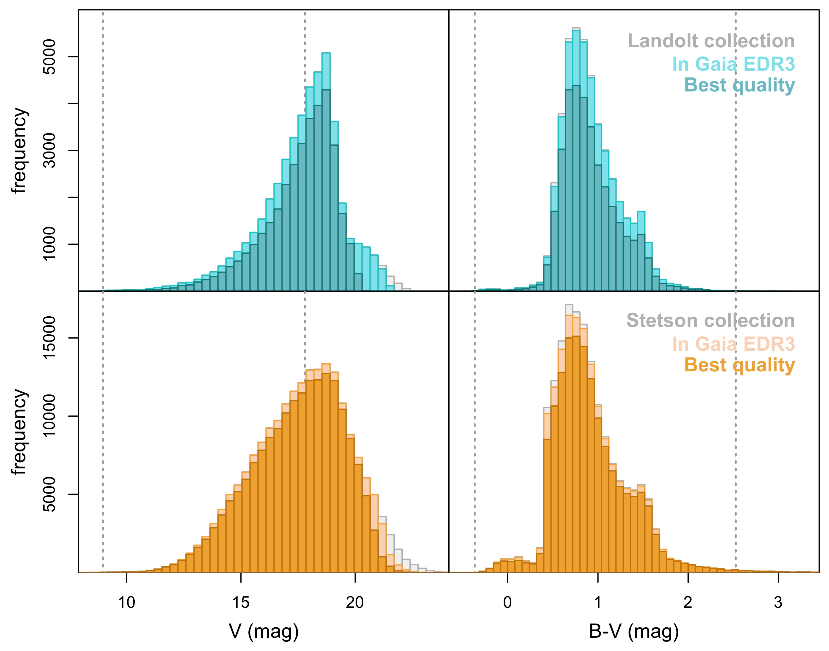
Figure 1: The V magnitude (left panels) and B-V color (right panels) distribution of the Landolt (top panels) and Stetson (bottom panels) collections. The full samples are plotted in grey, the samples with a match in Gaia EDR3 in light colors, and the best-quality samples (see Section 4.1 for details) in full colors. The dotted vertical lines show the coverage of the original Landolt (1992) standards set.

In this paper we build on the large body of exquisite measurements by A. U. Landolt, (Landolt & Uomoto 2007; Landolt 2007, 2009, 2013; Clem & Landolt 2013, 2016), P. B. Stetson and collaborators (Stetson & Harris 1988; Stetson 2000; Stetson et al. 2019), to provide a sample of more than 200 000 secondary standards, accurately calibrated on the original standards by Landolt (1992). The Landolt and Stetson collections have been curated, pruned of variable stars and binaries, and cross-matched – with the help of Gaia – to several large photometric surveys in different photometric systems. The two collections have also been characterized in terms of atmospheric parameters, reddening, distance, and therefore will hopefully enable a variety of calibration and inter-comparison tasks, including the calibration of Johnson-Kron-Cousins measurements from images that were not observed together with Landolt (1992) standard fields.

The paper is organized as follows: in Section 2 we present the Landolt and the Stetson collections; in Section 3 we describe the cross-match with Gaia and all the quality checks on the data, including the identification of binary and variable stars; in Section 4 we compare and combine the collections into one catalogue, and we characterize its stellar content in terms of distance, reddening, classification, and stellar parameters; in Section 5 we compute transformations between the Johnson-Kron-Cousins system and some other widely used photometric systems; finally, in Section 6 we summarize our results and draw our conclusions.

2 The Landolt and Stetson collections

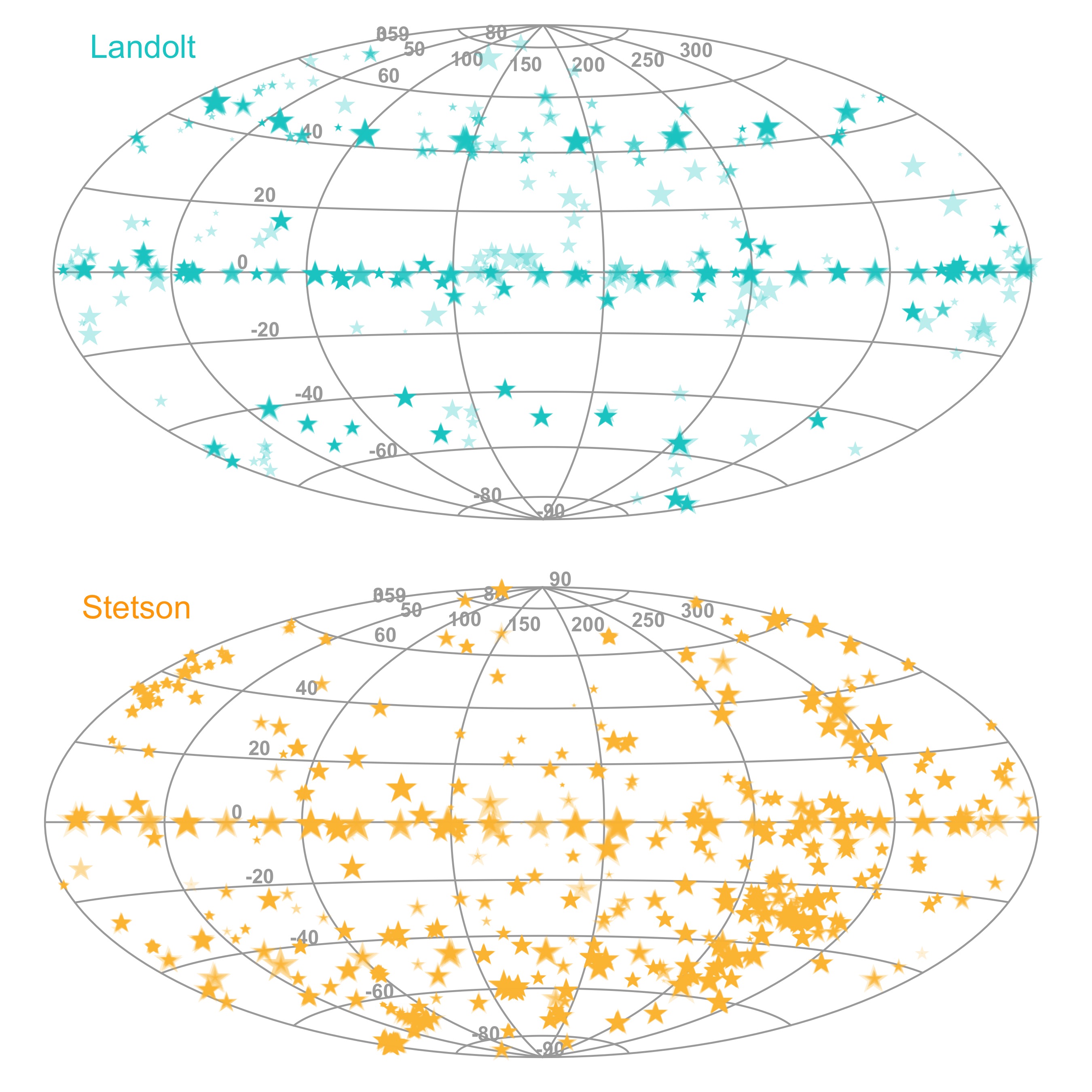
Figure 2: Distribution in RA and Dec on the sky of the Landolt (top panel) and Stetson (bottom panel) collections, in an Aitoff projection. Note that some of the Landolt fields are also included in the Stetson collection. The sizes of the symbols are proportional to the magnitudes and darker colors correspond to higher star densities.

Table 1: The curated Landolt collection (Section 2.1), with re-calibrated uncertainties and cross-match analysis parameters (Section 3.1). This table contains also 520 stars with no Gaia EDR3 match (Section 3.1), thus we report both the original Landolt coordinates and the Gaia EDR3 ICRS coordinates (epoch J2016), when available.

Column	Units	Description
Unique ID		Unique star ID defined here
Gaia EDR3 ID		Gaia Source ID from EDR3
Star Name		Landolt star name
RAorig	deg	Landolt original right ascension
Decorig	deg	Landolt original declination
RAEDR3	deg	Gaia EDR3 right ascension
DecEDR3	deg	Gaia EDR3 declination
U	mag	U-band magnitude
$\sigma$U	mag	re-calibrated uncertainty on U
nU		number of U-band measurements
B	mag	B-band magnitude
$\sigma$B	mag	re-calibrated uncertainty on B
nB		number of B-band measurements
V	mag	V-band magnitude
$\sigma$V	mag	re-calibrated uncertainty on V
nV		number of V-band measurements
R	mag	R-band magnitude
$\sigma$R	mag	re-calibrated uncertainty on R
nR		number of R-band measurements
I	mag	I-band magnitude
$\sigma$I	mag	re-calibrated uncertainty on I
nI		number of I-band measurements
PhotQual		Photometric quality flag
Duplicates		Number of duplicates ($\geq$0)
Neighbors		Number of neighbors ($\geq$1)
gaiaDist	arcsec	Distance from Gaia best match

2.1 The Landolt collection

The Landolt standards (Landolt 1992) are the foundation of the Johnson-Kron-Cousins photometric system. Although they are tied to the Vega zero-point, they are based on the sets of primary standards in UBV by Johnson (1963) and in RI by Cousins (1976). In practice, they were used for three decades to calibrate the vast majority of all imaging observations in the $UBVRI$ passbands. The original 1992 photoelectric set was later extended with observations far from the celestial equator and also with a large amount of CCD observations. We consider here a series of works by Landolt and collaborators, that can be divided into two subgroups: one based on photoelectric observations (Landolt 1992; Landolt & Uomoto 2007; Landolt 2007, 2009, 2013) and the other on CCD observations (Clem & Landolt 2013, 2016). We also complement the set with $UBVRI$ measurements for two CALSPEC (Bohlin 2014; Bohlin et al. 2019) standards by Bohlin & Landolt (2015). A preliminary version of the Landolt collection presented here was used to validate the Gaia Spectro-Photometric Standard Stars for the flux calibration of Gaia (hereafter SPSS; Pancino et al. 2012, 2021; Altavilla et al. 2015, 2021; Marinoni et al. 2016). A more advanced preliminary version of this collection was used to standardize the synthetic photometry obtained from the Gaia DR3 low-resolution spectra (R=$\lambda/\delta\lambda\simeq 20-100$, Gaia collaboration, Montegriffo et al., in preparation).

When assembling the Landolt collection, we always chose the most recent measurement in case of stars re-observed in different papers (see also Section 3.1). In general, newest photometry was based on larger numbers of independent measurements in each band. Detailed comparisons presented in the respective publications show that the measurements agree with the original Landolt (1992) ones and with each other to better than 1%, which is considered the current technological limit in our ability to calibrate the flux of stars (Clem & Landolt 2013; Bohlin et al. 2019; Pancino et al. 2021, see also Section 3.1 and Figure 3). Their photometry was made with a fixed aperture of 14” to replicate as much as possible the observing setup of the Landolt (1992) set. Small trends between the newer CCD measurements and the older photoelectric measurements were carefully corrected in the Clem & Landolt (2013, 2016) analysis, to follow as faithfully as possible the photometric system defined by the original Landolt (1992) standards. The collection contains about 47000 stars (see also Section 3.1), of which $\simeq$90% are from Clem & Landolt (2013, 2016). The distribution of the Landolt collection in magnitude and color is presented in Figure 1. The sky distribution is presented in Figure 2, where the original observations are clustered along the celestial equator, while recent observations populate the $\pm$50 deg declination strips and other areas on the sky.

We also evaluated the relative quality of the photometry by adding to each entry the PhotQual flag, which counts in how many passbands the star has uncertainties exceeding the 99th percentile of the uncertainty distribution as a function of magnitude. The curated Landolt collection, including indications about the number of duplicates and of neighbors from the cross-match analysis presented in Section 3.1, is presented in Table 1. The uncertainties in the curated Landolt collection have been re-calibrated as described in Section 3.1.

2.2 The Stetson collection

The Stetson database (Stetson 2000; Stetson et al. 2019) is based on more than half a million public and proprietary CCD images, collected by P. B. Stetson starting in 1983, when public archives did not exist yet. The images cover open and globular clusters, dwarf galaxies, supernova remnants, and other interesting areas on the sky, including some Landolt (1992) standard fields. All images were obtained in $UBVRI$ filters and were uniformly processed. Photometry was derived with the DAOPHOT package (Stetson 1987, 1994) and calibrated on the Johnson-Kron-Cousins system based on repeated Landolt (1992) standard field observations. It is worth noting that, unlike in the Landolt collection, the Stetson collection measurements were obtained by profile fitting, and then corrected with aperture photometry curves of growth. Only stars matching strict quality criteria were considered as secondary $UBVRI$ standards: (i) observed at least five times independently in photometric conditions, (ii) with uncertainties $<$0.02 mag, and (iii) with a spread in repeated measurements $<$0.05 mag (see Stetson et al. 2019, for more details). The Stetson database grows in time as new images are selected from public archives, and the quality of the measurements increases as more and more measurements contribute to the homogeneity and stability of the global photometric solution. Updates to the Stetson database are uploaded on a regular basis, therefore it is relevant to note that the data presented here were downloaded in April, 2021 and consists in more than 200 000 entries (see also Section 3.2).

The Stetson secondary standards are routinely used to calibrate photometry when no accurate standard stars observations were obtained, or to compute transformations between catalogues when no stars in common with the Landolt collection are found. For example, they were used to calibrate the photometry for the Gaia-ESO calibrating clusters observations (Gilmore et al. 2012; Pancino et al. 2017); the 2019 version of the standards was used, among other catalogues, by Riello et al. (2021) to validate the Gaia EDR3 photometric calibration and to derive color transformations between the Gaia and Johnson-Kron-Cousins photometry; and the transformations used to build the all-sky PLATO input catalogue (asPIC1.1) were based, among other sets, on the Stetson secondary standards as well (Montalto et al. 2021).

Table 2: The curated Stetson collection (Section 2.2), with cross-match analysis parameters (Section 3.2), and re-calibrated uncertainties (Section 4.2). The number of measurements reported here for each band refers to measurements obtained in photometric sky conditions only, according to the original Stetson data tables. This table contains also 4970 stars with no Gaia EDR3 match, thus we report both the original coordinates from Stetson and the Gaia EDR3 ICRS coordinates (epoch J2016), when available.

Column	Units	Description
Unique ID		Unique star ID defined here
Gaia EDR3 ID		Gaia Source ID from EDR3
Star Name		Stetson star Name
RAorig	deg	Stetson original right ascension
Decorig	deg	Stetson original declination
RAEDR3	deg	Gaia EDR3 right ascension
DecEDR3	deg	Gaia EDR3 declination
U	mag	U-band magnitude
$\sigma$U	mag	re-calibrated uncertainty on U
nU		Number of U-band measurements
B	mag	B-band magnitude
$\sigma$B	mag	re-calibrated uncertainty on B
nB		Number of B-band measurements
V	mag	V-band magnitude
$\sigma$V	mag	re-calibrated uncertainty on V
nV		Number of V-band measurements
R	mag	R-band magnitude
$\sigma$R	mag	re-calibrated uncertainty on R
nR		Number of R-band measurements
I	mag	I-band magnitude
$\sigma$I	mag	re-calibrated uncertainty on I
nI		Number of I-band measurements
VarWS		Welch-Stetson variability index
PhotQual		Photometric quality flag
Duplicates		Number of duplicates ($\geq$0)
Neighbors		Number of neighbors ($\geq$1)
gaiaDist	arcsec	Distance from Gaia best match

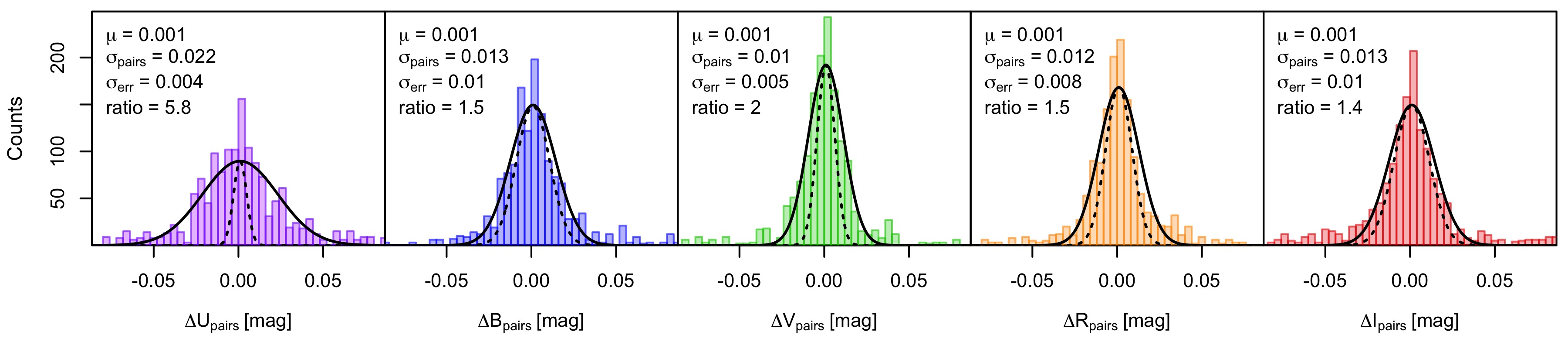
Figure 3: Analysis of the 1532 duplicated measurements in the Landolt collection, for 679 stars. Each panel displays the paired magnitude differences in a different band. Solid lines are Gaussians centered on the mean difference $\mu$ and standard deviation equal to the MAD (median absolute deviation) of the paired differences $\sigma_{\rm{pairs}}$. Dashed lines show Gaussians centered on $\mu$ and with a standard deviation obtained by summing in quadrature the Landolt uncertainties of the stars in each pair, $\sigma_{\rm{err}}$. The ratios between the two standard deviations are annotated in each panel, along with relevant quantities.

Before proceding, we used the photometric uncertainties in the Stetson collection to trim the stars with relatively worse photometric quality. We defined a quality flag (PhotQual in Table 2) similarly to what done for the Landolt collection: we counted the number of bands in which the photometric error is higher than the 99th percentile, as a function of magnitude. Besides the magnitudes, errors, and the number of measurements in each band, the Stetson original catalogues contain an indication of the probability that a star is variable (VarWS in Table 2), which is derived from the Welch-Stetson variability index (Welch & Stetson 1993; Stetson et al. 2019) and the number of available measurements (see also Section 3.2). To further clean the sample, we increased the above photometric flag by one for the stars in the extreme tail of the variability flag distribution (VarWS$>$0.04, 1588 stars). The resulting catalogue of unique secondary standards in the Stetson collection, including coordinates, photometry, quality parameters, and the cross-match analysis flags (from Section 3.2), is presented in Table 2 (see also Figures 1 and 2). The errors are re-calibrated following the analysis in Section 4.2.

3 Gaia cross-match and catalogue cleaning

We cross-matched the Landolt and Stetson collections with Gaia (Gaia Collaboration et al. 2016) EDR3 data (Gaia Collaboration et al. 2021) and with additional literature catalogues (Section 4). As a result, we cleaned the sample from duplicates and unreliable matches and we flagged suspect binaries and variable stars, or stars with relatively lower quality in their photometry.

We employed the Gaia cross-match software, routinely used to produce cross-identifications of Gaia sources within large public surveys (Marrese et al. 2017, 2019). The version of the software adopted here (Marrese et al. 2019) finds the best matching Gaia source(s) given an external sparse catalogue, i.e., in our case the Landolt or the Stetson collection. For each source, a figure of merit is computed after correcting stellar position for the proper motions and epoch of the observations, that takes into account all the relevant uncertainties as well as the Gaia local stellar density. The software also helps in finding: (i) likely duplicates, i.e., stars in the sparse catalogue that point to the same Gaia star and (ii) neighbors, i.e., additional Gaia stars that have compatible positions with an object in the sparse catalogue.

We also performed a cross-match between the Gaia DR2 and EDR3 releases, with the source IDs reported in Table 5. This differs from the official Gaia DR2-EDR3 match in the sense that we looked backwards for EDR3 stars in the DR2 catalogue, while the official Gaia cross-match looks forward for DR2 stars in the EDR3 catalogue. This specific cross-match will be used below for the cross-match with the Survey of Surveys SoS (Tsantaki et al. 2022, see also Sections 3.5 and 4.5) and for the reddening estimates (Section 4.3).

3.1 Landolt cross-match analysis

For the Landolt collection, we found 563 stars without a match, of which 520 are too faint to be in Gaia (V$>$20.5 mag). For the remaining 43, which were mostly bright, high-proper motion stars, we performed manually wide cone searches (up to 5–35”) and ultimately recovered them all. All of the duplicated entries found during the cross-match (679 stars with 1532 entries) came from different source papers, i.e. there were no unrecognized duplicates in any of the individual source catalogues. Among stars repeated in different papers, about a dozen pairs had large magnitude differences ($>$0.3 mag), generally in the U and B bands, but they all had very few measurements in the oldest of the source catalogues. Apart from these cases, we found that the typical spreads in the pairwise magnitude differences was about 1–2% (Figure 3), depending on the band. The spreads of the paired differences were generally not compatible with the squared sum of the formal uncertainties on each pair, being on average larger by a varying amount. We thus multiplied the original Landolt uncertainties by the ratios reported in Figure 3, i.e., 5.8 for the U band, 1.5 for the B and R bands, 2 for the V band, and 1.4 for the I band. The re-calibrated uncertainties are reported in Table 1. Stars with repeated entries in different Landolt source catalogues were flagged (Duplicates column in Table 1).

The resulting catalogue of unique stars contained 683 stars with one or more neighbors, i.e., with possible alternate matches, albeit with a lower figure of merit (as defined by Marrese et al. 2019). To verify whether any neighbor could be a better match than the originally chosen best match, we computed the expected G magnitude from Landolt V and V–I, using both the relations by Riello et al. (2021) and the ones presented in Section 5.1, and we studied the distribution of differences between the original and expected Gaia magnitudes. On the one hand, we found that neighbors were generally fainter in Gaia than expected from the V and I magnitudes in the Landolt collection. On the other hand, the best matches had expected G magnitudes compatible with the V and I Landolt magnitudes, within uncertanties. We thus concluded that the best matches – according to the astrometric figure of merit – were also best matches according to photometry. Therefore, we kept the best match in the catalogue, but we flagged all stars with neighbors (Neighbors column in Table 1).

3.2 Stetson cross-match analysis

For the Stetson collection, the database snapshot downloaded in April 2021 contains 204 303 individual entries. In the field of the Carina dwarf galaxy, we found almost 5000 stars with the same ID and photometry, and slightly different coordinates. These duplicates were removed before performing the cross-match and are not included in the figure above. Of the 4970 stars without a Gaia match, about 4550 are too faint to be observed by Gaia, while the remaining $\simeq$450 are mostly located in the Hydra I cluster field. Even when trying a wide cone search (20”) and then selecting the best neighbors based on magnitudes, we could not recover unambiguously these stars in the Gaia catalogue.

Only one unrecognized duplicate object was found in the Stetson collection, thus no independent statistical analysis of the reported uncertainties was possible. We therefore used the comparison with the Landolt collection to re-calibrate the Stetson uncertainties, which are reported in Table 2 (see Section 4.2 for details). The stars with at least one neighbor are 19073 and the number of neighbors is reported in the Neighbors column in Table 2. Similarly to the case of the Landolt collection, the neighbors do not only have a lower figure of merit based on their positions and motions, but they also tend to have Gaia magnitudes systematically fainter than expected from their V and I magnitudes, using both the relations by Riello et al. (2021) and our own relations from Section 5.1. Conversely, the best matches have compatible measured and expected Gaia magnitudes, within uncertainties. Therefore, we kept the best matches in all cases.

3.3 Gaia photometric quality flag

The precision and accuracy of the Gaia EDR3 photometry is unprecedented, especially for the relatively bright stars in common with the Landolt and Stetson collections presented here: standard errors of a few mmag or better and an overall zeropoint accuracy of better than 1% (Riello et al. 2021; Pancino et al. 2021). Thanks to the numerous parameters published in the Gaia catalogue, we can perform a variety of quality assessments. In the next section we will deal with the risk of contamination and blends by nearby stars and binary companions. Here, we will use those parameters that are most relevant to evaluate the photometric measurement quality. We started by flagging (not removing) stars with:

• a BP magnitude lower than 20.3 mag, following the recommendation by Riello et al. (2021);

• a two-parameter solution, i.e., without proper motion and parallax determination (Lindegren et al. 2021b) and, what is more important here, without BP and RP magnitudes;

• a relative error on the flux of the G, G_BP, and G_RP magnitudes larger than the 99th percentile as a function of magnitude, similarly to what done in Sections 2.1 and 2.2 for the ground-based photometric quality;

• a fraction of BP or RP contaminated transits higher than 7% (following Riello et al. 2021), indicating that the mean photometry could be significantly disturbed by nearby (bright) stars, located outside of the BP/RP window assigned to the star itself.

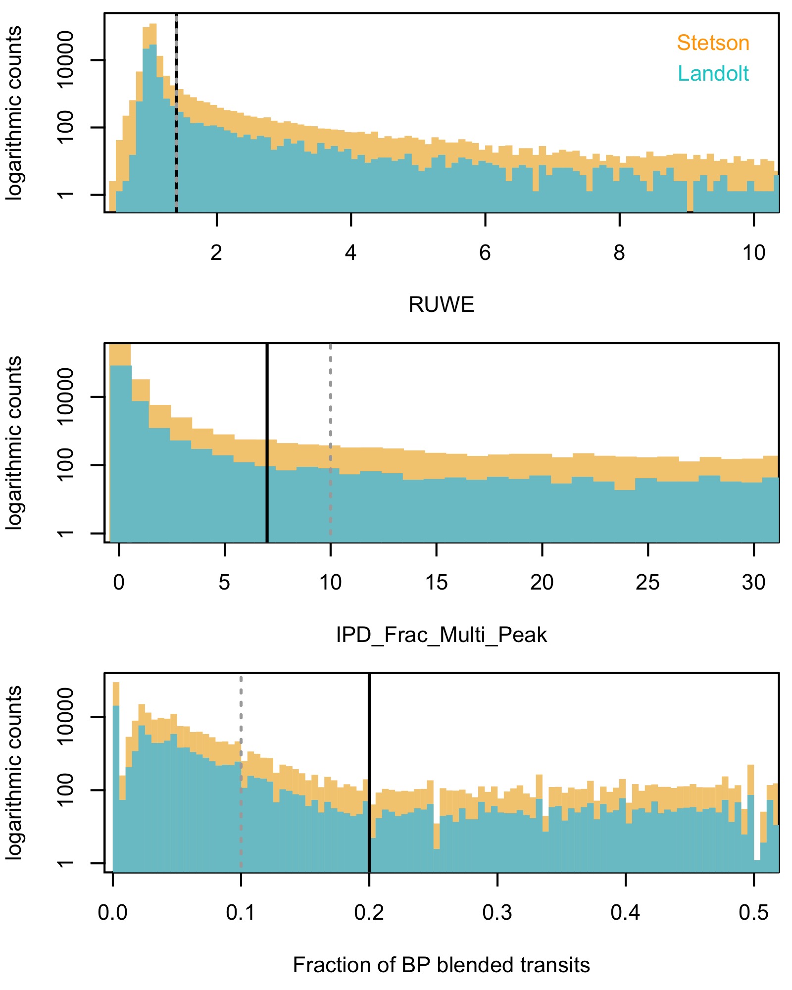
Figure 4: Example of quality thresholds: each panel shows the logarithmic histogram of some of the explored Gaia EDR3 parameters, for the Landolt (cyan) and Stetson (orange) collections. The recommended thresholds by Lindegren et al. (2021b), Fabricius et al. (2021), and Riello et al. (2021) are indicated by grey dotted vertical lines, while our final adopted ones are indicated by black solid lines.

In practice, the Gaia quality flag GaiaQual (Table 5) counts how many of the above quality criteria were not fulfilled, i.e., a zero flag means that all criteria were passed (best quality), one that one quality criterium was not met, and so on. In the Landolt collection, 98% of the stars with a Gaia match met all the quality criteria, while no star failed all the criteria. In the Stetson collection, 82% of the stars with a Gaia match passed all the quality criteria, while only one star failed all criteria.

3.4 Probable blends and binaries

As a space observatory with a typical PSF (Point Spread Function) size of 0.177”, Gaia can help in flagging potentially disturbed sources, either by chance superposition with other stars on the plane of the sky (blends) or by gravitationally bound binary companions. Among the astrometric quality indicators in the Gaia EDR3 main catalogue (Lindegren et al. 2021b; Fabricius et al. 2021), we used the following for the purpose:

• IPDFracOddWin is the fraction (in percentage) of Gaia transits that had disturbed windows or gates, indicating that those transits are likely to be contaminated by a possible companion (or a spurious source); we conservatively flagged all stars with more than 7% of disturbed transits;

• IPDFracMultiPeak is the fraction (in percentage) of the Gaia transits with double or multiple peaks detected in the PSF; we conservatively flagged all stars with more than 7% of multiple-peak transits (Figure 4, see also Mannucci et al. 2022, where this indicator was used to reliably select double QSO candidates with separations of 0.3”-0.6”);

• RUWE is the renormalized unit weight error of the astrometric solution; for well behaved stars it should be around one and Lindegren et al. (2021b) suggested a cut of $<$1.4, which seems appropriate for our sample as well (Figure 4);

• the fraction of BP and RP with blended transits, i.e. with one or more disturbing sources within the BP/RP window assigned to the star, is also a useful indicator (Riello et al. 2021); we flagged stars with more than 20% of blended transits in BP or RP (Figure 4);

• finally, we computed the C* parameter, a color-corrected version of the bp_rp_excess_factor (Riello et al. 2021); when higher than zero, it indicates that the sum of the BP and RP fluxes is higher than the G-band flux, indicating a possible flux contamination by nearby sources; when smaller than zero, the opposite is true, for example because of background over-subtraction in BP or RP. We applied a threshold to C* following the modeling of $\sigma_{\rm{C*}}$ by Riello et al. (2021, Section 9.4), and we flagged all sources with $|\rm{C*}|>2\,\sigma_{\rm{C*}}$.

Similarly to what was done in the previous section, the GaiaBlend flag (Table 5) indicates the number of the above criteria that failed. Thus, a flag of zero means that the star passed all criteria, while a flag of $n$ means that it failed $n$ criteria. In the Landolt collection, 85% of the stars met all criteria, while 13 stars failed them all. In the Stetson collection, 85% of the stars met all criteria, while 39 stars failed them all.

Table 3: Dictionary for the stellar classification labels in the StarType column in Tables 4 and 5. A colon ”:” added after the Acronym in the StarType column indicates an uncertain or suspected classification.

Acronym	Description
BYDRA	BY Draconis type rotational variables
CB	Close Binary
CnB	Contact binary
COOL	Cool Main Sequence star, mostly K or M
DCEP	Classical Cepheid variable ($\delta$ Cephei type)
DSCT	Low-amplitude $\delta$ Scuti type variables)
EA	Detached Algol-type binary
EB	$\beta$ Lyrae type binary
EW	W Ursa Majoris type binary
GCAS	$\gamma$ Cassiopeiae type variable (rapidly rotating
	early type stars with mass outflow)
HOT	Hot star, mostly OBA main sequence
HOT_SD	Hot Sub-dwarf
L	Red irregular variable
LP	Long period variable
LPSR	Long period semi-regular variable
MIRA	Mira type variable
MS	Main Sequence Star, mostly AFGK
PN	Central star of a Planetary Nebula
R	Rotational variable
RG	Red giant star
RC	Red clump star
RRAB	RR Lyrae with asymmetric light curves,
	fundamental mode
RRC	RR Lyr with nearly symmetric light curves,
	first overtone
RRD	Double Mode RR Lyrae variables
ROT	Spotted stars showing rotational modulation
RSCVN	RS Canum Venaticorum rotational variables
SB1	Single-lined spectroscopic binary
SB2	Double-lined spectroscopic binary
SBVC	Spectroscopic binary or variable candidates
SD	Sub-dwarf
SR	Semi-regular variable
T2CEP	Type II Cepheid (no sub-classification)
T2CEP_WVIR	W Virginis type variables (Cepheid)
UGER	ER Ursae Majoris cataclysmic variables
UV	Flare star
UWB	Ultra-wide binary
V361HYA	V361 Hydrae type variable stars
	(fast pulsating hot subdwarf)
VAR	Variable star of unspecified type
WD	White Dwarf
YSO	Young Stellar Object (irregular variable)
ZZCET	ZZ Ceti type variable star (WD variable)

3.5 Binary stars

To identify spectroscopically confirmed binaries, we used the Survey of Surveys (hereafter SoS, Tsantaki et al. 2022), which combines in a homogeneous way data from the major spectroscopic surveys (see Section 4.5 for more details). Among other parameters, the SoS catalogue contains a flag indicating whether a star is a spectroscopic confirmed binary in any of the surveys, using information from Price-Whelan et al. (2020) and Kounkel et al. (2021) for APOGEE, Traven et al. (2020) for GALAH, Merle et al. (2017) for Gaia-ESO, Birko et al. (2019) for RAVE, Qian et al. (2019) for LAMOST, and Tian et al. (2020) for Gaia DR2. Because the SoS is based on Gaia DR2, we used the Gaia DR2-EDR3 cross-match described at the beginning of Section 3. In addition, we also searched the CoRoT (Deleuil et al. 2018) and the Kepler (Kirk et al. 2016) catalogues for binary stars.

As a result, we found 301 unique confirmed binaries (308 when counting detections in multiple catalogues), of which 35 from the Landolt collection and 266 from the Stetson collection. About half of the 301 stars are classified as close binaries by APOGEE (Price-Whelan et al. 2020; Kounkel et al. 2021), the others are SB2, contact binaries, radial velocity variables, or ultra-wide binaries. We have set a flag for these stars, BinFlag=1, in Table 5. Their classification, according to the dictionary in Table 3, is stored in the StarType column in Table 5, with an annotation in the StarMethod column stating ”Binary – see Table 4”. Of the found binaries, 16 were also classified as variable stars (next section), thus we included both the binary and the variable classification in the starType column of Table 5, separated by a slash. More details on their classification and literature source can be found in Table 4. The spectroscopically confirmed binaries, which dominate by number the found binaries, have orbital plane inclinations that tend to be parallel to the line of sight. This makes them complementary to the suspected astrometric binaries, flagged with GaiaBlend=1 together with photometric blends, whose orbital planes tend to be perpendicular to the line of sight.

Table 4: Details on notable stars with non-zero VarFlag and/or BinFlag in Table 5. Stars found in more than one external catalogue have repeated entries in this table.

Column	Description
Star ID	Star ID from Table 5
Gaia EDR3 ID	Gaia Source ID from EDR3
External ID	ID in the external catalogue
Source	External catalogue
StarType	External classification (Table 3)
	(”:” means suspected or uncertain)
Notes	Any additional notes

3.6 Variable stars

To search for variable stars in the Landolt and Stetson collections, we examined three different catalogues: (i) the Gaia DR2 catalogue of variable stars (Gaia Collaboration et al. 2019); (ii) the ASAS-SN catalogue of variable stars (Shappee et al. 2014; Jayasinghe et al. 2018, 2019a, 2019b); and (iii) the The Zwicky Transient Facility (ZTF) catalog of periodic variable stars (Chen et al. 2020). When appropriate, we used our Gaia DR2-EDR3 cross-match to identify the stars in the various catalogues.

We found 117 variables in the Landolt collection and 1416 in the Stetson collection (but see Section 4.4 for additional identifications of young stellar objects). The majority were unclassified variables ($\simeq$900), followed by rotational variables ($\simeq$250). There were 19 variables in common between the Gaia DR2 and the ASAS-SN catalogue, 37 between ZTF and ASAS-SN, 5 between Gaia DR2 and ZTF, and only one star was reported as variable in all three catalogues. To classify variable stars present in more than one catalogue, we adopted the following choices:

• when the variability class was certain in one catalogue and uncertain in another (with a colon ”:” appended), we chose the certain one (i.e., ROT over ROT:);

• if all classifications were uncertain, but one specified a class, we chose the more specific one (i.e., ROT: over VAR:);

• if two or more classifications were concordant, we chose the most specific one or the one indicating the subcategory (i.e., ROT over VAR, or RSCVN over ROT);

• if classifications were discordant at any level (category or sub-category) we indicated them all separated by a slash (i.e., EW/EB).

A dictionary of all the adopted StarType labels can be found in Table 3. In the main combined catalogue (Table 5), we just indicated whether the star is a variable using the column VarFlag, that is zero for non-variable stars and one for variable stars; the variable type was indicated in the StarType column and the star was excluded from the clean sample (Qual=1). In that table, the StarMethod column reports the string ”Variable – see Table 4”. We then provided more details in Table 4, where stars identified as variables in multiple catalogues have multiple entries, and the original classification from the corresponding literature source is reported in StarType for each entry.

We note here that some of the confirmed or suspected variables in the Landolt collection are part of some of the most widely used selected areas, for example around Mark A, Ru 152, T Phe, some of the PG standards, and in the SA98, SA104, SA107, SA110, and SA113 standard fields.

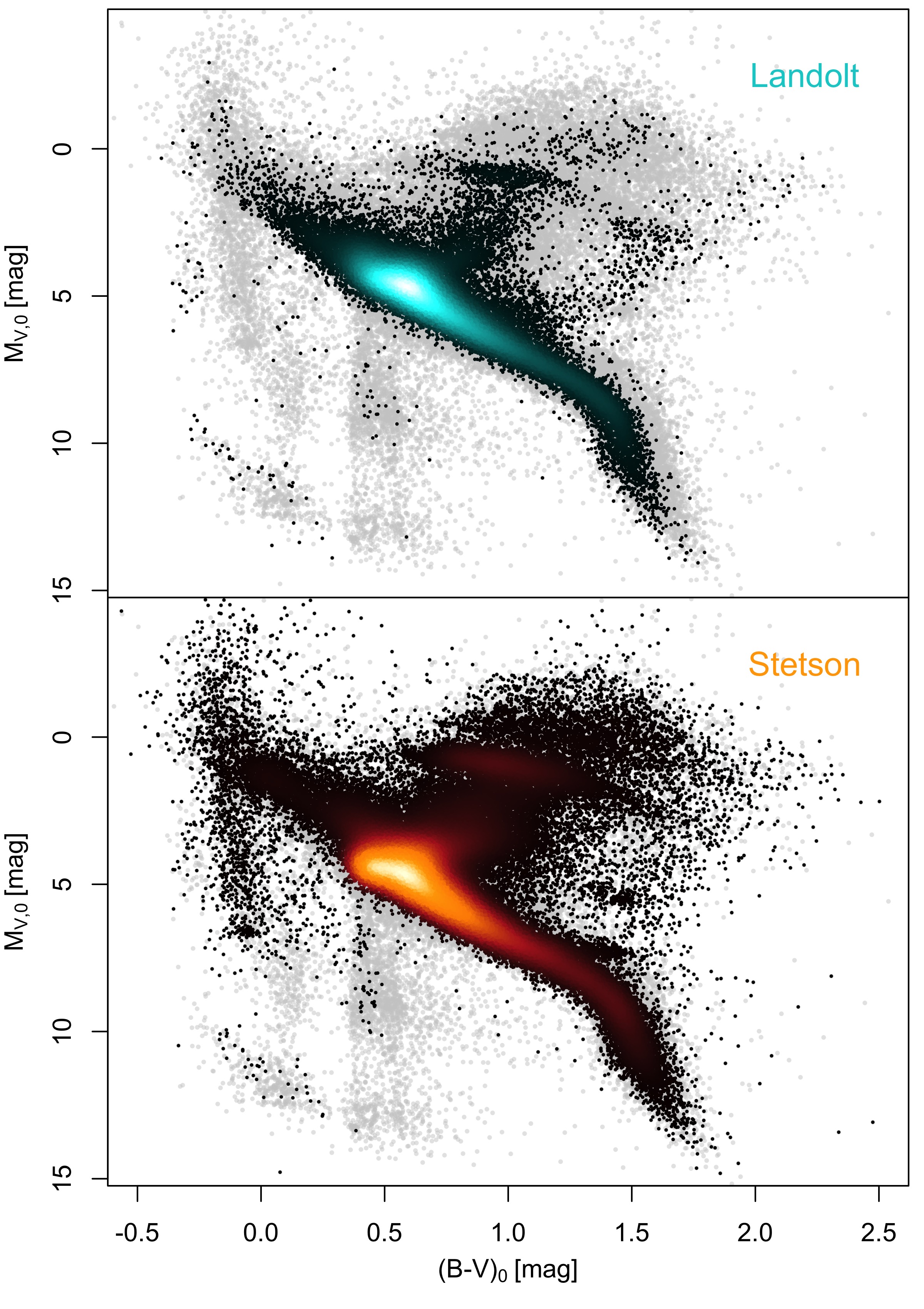
Figure 5: The clean Landolt (top panel) and Stetson (bottom panel) samples, in the absolute and de-reddened V, B–V plane. Stars belonging to both the Landolt and the Stetson collections are only shown in the top panel. The color scales reflect the density of points in the CMD. The whole sample of stars with distance and reddening estimates (Section 4.3, Table 5) is reported in both panels as grey dots in the background. The vertical stripes of stars between the main sequence and the white dwarfs, that almost disappear in the clean samples, are mostly made of relatively faint stars with very uncertain distance estimates.

Table 5: Content of the combined secondary standards catalogue.

Column	Units	Description
Unique ID		Unique star ID defined here
EDR3 ID		Gaia Source ID from EDR3
DR2 ID		Gaia Source ID from DR2
Star Name		Star Name
Collection		Landolt or Stetson
RAorig	deg	Original right ascension
Decorig	deg	Original declination
RAEDR3	deg	Gaia EDR3 right ascension
DecEDR3	deg	Gaia EDR3 declination
U	mag	U-band calibrated magnitude
$\sigma$U	mag	uncertainty on U
nU		Number of U-band measurements
B	mag	B-band calibrated magnitude
$\sigma$B	mag	uncertainty on B
nB		Number of B-band measurements
V	mag	V-band calibrated magnitude
$\sigma$V	mag	uncertainty on V
nV		Number of V-band measurements
R	mag	R-band calibrated magnitude
$\sigma$R	mag	uncertainty on R
nR		Number of R-band measurements
I	mag	I-band calibrated magnitude
$\sigma$I	mag	uncertainty on I
nI		Number of I-band measurements
PhotQual		Photometry quality (Section 2.1, 2.2)
GaiaQual		Gaia quality (Section 3.3)
GaiaBlend		Suspect blend or binary (Section 3.4)
BinFlag		Binary flag (Section 3.5, Table 4)
VarFlag		Variable flag (Section 3.6, Table 4)
Qual		Clean sample has zero (Section 4.1)
Dist	(pc)	Distance (Section 4.3)
Distmin	(pc)	Minimum distance (Section 4.3)
Distmax	(pc)	Maximum distance (Section 4.3)
E(B–V)	(mag)	Reddening (Section 4.3)
$\sigma$E(B–V)	(mag)	Reddening error (Section 4.3)
StarType		Classification (Section 4.4, Table 3)
StarMethod		Classification method (Section 4.4)
RV	(km/s)	Line-of sight velocity (Section 4.5)
$\sigma$RV	(km/s)	RV error (Section 4.5)
RVMethod		Source of the RV
Teff	(K)	Effective temperature (Section 4.5)
$\sigma$Teff	(K)	Teff error (Section 4.5)
log$g$	(dex)	Surface gravity (Section 4.5)
$\sigma$log$g$	(dex)	log$g$ error (Section 4.5)
$\rm{[Fe/H]}$	(dex)	Iron abundance (Section 4.5)
$\sigma\rm{[Fe/H]}$	(dex)	[Fe/H] error (Section 4.5)
ParMethod		Method for Teff, log$g$, and [Fe/H]
		(Section 4.5)

4 The combined catalogue

We detail in the following sections our procedures to generate the final combined catalogue: we first define a clean sample (Section 4.1); we then compare the Landolt and Stetson collections before merging them (Section 4.2); we further proceed to characterize the stars in terms of reddening, distance, stellar type, and astrophysical parameters (Sections 4.3, 4.4, 4.5). A summary of the catalogue content and format can be found in Table 5, which will be available electronically and will also be published at the CDS through the Vizier service and at SSDC through the GaiaPortal service.

4.1 Clean sample

Before proceeding, we build a clean sample, that will be used in the following analysis and especially in Section 5. Note that all stars will be listed in the combined catalogue, not just the ones belonging to the clean sample. We use the criteria:

• the photometric quality flags (PhotQual) in the Landolt (Section 2.1, Table 1) and Stetson collections (Section 2.2, Table 2) must be smaller than three, meaning that the star cannot be an outlier in three bands or more;

• the Gaia photometric quality flag GaiaQual must also be smaller than three (Section 3.3);

• the Gaia suspected blends and binaries flag GaiaBlend (Section 3.4) must be zero and the star must not be a confirmed binary (i.e., BinFlag=0) in any of the scanned binary star catalogues (Section 3.5);

• the star is not a suspected or confirmed variable (VarFlag and Section 3.6) and in particular is not a suspected or confirmed YSO (see also Section 4.4);

• as an important exception, the ten reddest stars (V–I$>$3.5 mag) in the Landolt collection with a Gaia match are kept for the following analysis, regardless of their quality flags, because of the paucity of very red stars in the combined collection.

The clean Landolt and Stetson samples are shown in Figure 5. The Landolt clean sample contains 35194 stars (i.e., 76%), while the Stetson one 127467 stars (i.e., 67%), excluding those in common with the Landolt collection. The final combined catalogue (Table 5) contains a unified Qual flag that is zero for the clean sample, null for stars without a Gaia match, and one for the remaining stars.

4.2 Comparison and catalogue merging

The Landolt and Stetson collections are accurately calibrated on the original Landolt (1992) set of standards, which covers the color range –0.37$<$(B–V)$<$2.53 or –0.53$<$(V–I)$<$3.68 mag, with few stars in the bluest and reddest ranges. Thus, stars out of these color ranges are calibrated in extrapolation and might be less reliably placed on the standard system, and stars close to the color limits can also be uncertain, because their calibration is based on a handful of standards. In the Landolt collection, the red color limit is extended by about 0.5 mags with respect to Landolt (1992), while in the Stetson collection by about one magnitude. This has to be taken into consideration when comparing the two collections with each other. For the comparison, we used stars in common between the Landolt and Stetson collections, that matched the clean-sample criteria in Section 4.1: we found 10769 clean-sample stars in common between the two collections. The comparison is shown in Figure 6.

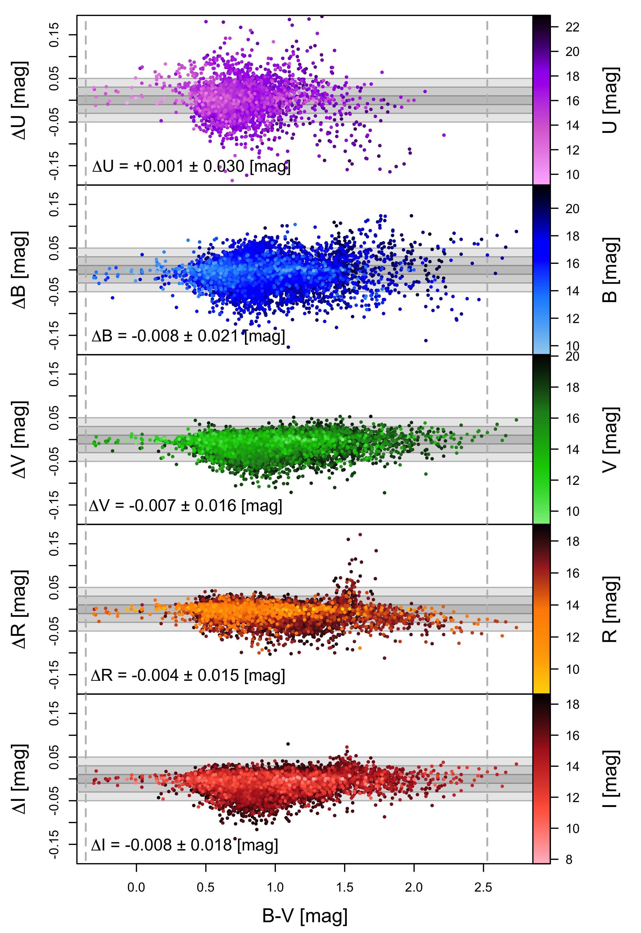
Figure 6: Differences between the Stetson and the Landolt magnitudes for 10769 stars in common, matching the clean-sample criteria (Section 4.1). Each panel reports one of the $UBVRI$ magnitudes as a function of the Landolt B-V, as indicated. The points are colored based on the respective Landolt magnitude, and the median differences with their median absolute deviations are reported in each panel. Horizontal lines and grey-shaded areas mark the zero, $\pm$1, $\pm$3, and $\pm$5% differences. Vertical lines mark the color range covered by the original Landolt (1992) catalogue, which defines the Johnson-Kron-Cousins system. The tail of faint stars extending upwards in the $\Delta$R panel at about B–V=1.5 mag is composed by M dwarfs (although other M dwarfs are well behaved) and could be populated by H${\rm{\alpha}}$ emitting stars.

Given that we could not renormalize the Stetson collection uncertainties because there was only one duplicated measurement, we can use this comparison instead. If we use the mean renormalized Landolt uncertainties in each band $\sigma_{\rm{Lan}}$ (Section 3.1) and the spread in the above comparisons $\sigma_{\rm{comp}}$, we can obtain the expected uncertainty in the Stetson collection, $\sigma_{\rm{Ste}}$ considering that $\sigma_{\rm{comp}}^{2}=\sigma_{\rm{Lan}}^{2}+\sigma_{\rm{Ste}}^{2}$. We thus find that the Stetson uncertainties are underestimated by approximately a factor of two. The re-calibrated uncertainties for the Landolt and Stetson collections are listed in Tables 1 and 2, and in the combined catalogue as well (Table 5).

As expected, the two collections agree to better than 1% with each other in each band, with a spread of 1–3% depending on the band. The U band has the highest spread of about 3%, while the B band displays a spread of 2%, with several discrepant stars. The bluest bands are notoriously more difficult to standardize (Clem & Landolt 2013; Altavilla et al. 2021; Pancino et al. 2021) and, in addition, the Stetson collection is based on a heterogeneous collection of data from different instruments and filter sets. As anticipated, we can observe a slightly worse agreement (at the 2–3% level) between the Landolt and Stetson collections for stars redder than B–V$\simeq$2 mag, especially in the R and I bands. The disagreement appears to be systematic, i.e., it seems to increase with color, and is most probably a consequence of the scarcity of red stars in the original Landolt (1992) catalogue, as discussed above. After several experiments, we decided not to re-calibrate the R and I magnitudes of the Stetson or Landolt collections, because different calibrations would be required to achieve a better agreement for the M dwarfs and the M giants. However, extra caution should be used when relying on stars redder than B–V$\simeq$2.0–2.5 mag.

For the final, combined catalogue, we chose the Landolt magnitudes when available and the Stetson magnitudes when the Landolt ones were missing. All the stars are listed in the combined catalogue, including those lacking a Gaia counterpart and those not matching the clean-sample criteria described in Section 4.1.

4.3 Distance and reddening

We complemented the combined catalogue with distance and reddening estimates. For Distances, we used the catalogue by Bailer-Jones et al. (2021), based on the Gaia EDR3 parallaxes, who carefully accounted for the relevant parallax biases (Lindegren et al. 2021b, a). We used their photo-geometric determination, which takes into account the expected color and magnitude distribution of stars in the Milky Way, to better constrain probable distances. The typical (median) distance is 2883 pc, while only about 25% of the stars are farther than 4883 pc. It is worth noting that the Stetson collection contains more distant stars compared to the Landolt collection, because it targets specifically globular clusters and dwarf galaxies with long exposures. We could assign a distance estimate to 96% of the stars in the combined collection, but for distant stars the uncertainties are of course rather high, with 25% of the stars having distance uncertainties above 40%.

For reddening, we explored two different sources: (i) the 3D reddening map by Green et al. (2019), based on Gaia DR2, Pan-STARRS 1 (Chambers et al. 2016; Flewelling 2016), and 2MASS (Skrutskie et al. 2006; Cutri et al. 2012); and (ii) the 3D reddening map by Lallement et al. (2019), based also on Gaia DR2 and 2MASS data. We used the 3D bins in the Green et al. (2019) and Lallement et al. (2019) maps to assign a reddening estimate to each of the stars in the Landolt and Stetson collections having a distance estimate in Bailer-Jones et al. (2021). For more distant stars, or stars with large distance uncertainties, which spanned more than one 3D-bin in the maps, we apdoted the weighted average of the E(B–V) estimates corresponding to the best distance estimate, the minimum distance estimate, and the maximum one. As a result, our E(B–V) estimates often have considerably larger uncertainties than the single 3D-bin values in the original reddening maps. We studied the differences between the E(B–V) values derived in this way from the Green et al. (2019) and the Lallement et al. (2019) maps. We found that – except for about 8% nearby stars with tendentially blue colors and located in specific areas of the sky – the two sets agree very well, with a median offset of 0.01$\pm$0.05 mag and a mean one of 0.02$\pm$0.14 mag. However, the Green et al. (2019) set does not cover the entire sky. We therefore decided to use the Lallement et al. (2019) maps for sake of homogeneity. We could assign an E(B–V) estimate to 96% of the stars in the combined catalogue, i.e., virtually all the stars with a distance estimate. It is however very important to keep in mind that a large fraction of the stars in the combined catalogue are farther than the volume covered by the 3D maps and therefore their E(B–V) might be underestimated.

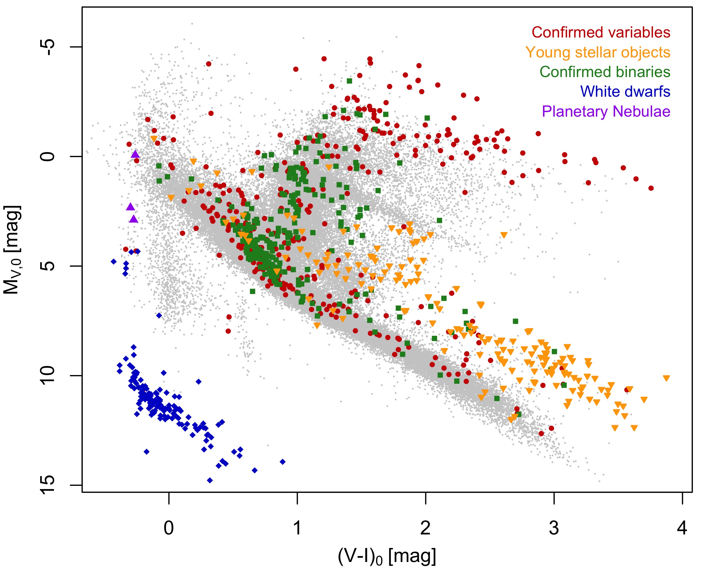
Figure 7: The position of some stellar types in the absolute and dereddenend V, V–I plane (see Sections 3.5, 3.6, and 4.4 for more details). The clean sample (Section 4.1) is plotted in grey in the background.

4.4 Color-magnitude diagram and stellar classification

To characterize the stellar content of the combined catalogue, we built the absolute and de-reddened color-magnitude diagram (CMD, see Figure 7), using the distance and the E(B–V) determined in Section 4.3. We assumed $R_{V}=3.1$ and used Dean et al. (1978) and Cardelli et al. (1989) to obtain A_λ/A_V from E(B–V). As a first step, we performed a rough manual classification of stars in different categories (main sequence, giants, red clump giants, hot, cool, subdwarfs, white dwarfs, and so on) based on their position in the above CMD, as indicated in the StarType column in Table 5, using the labels in Table 3. Only stars having V and I magnitudes, as well as distance and reddening estimates, could be initially classified this way. In the same StarType column, we also marked the following specific stellar types from literature catalogues:

• five central stars of confirmed planetary nebulae, identified with the catalogue by González-Santamaría et al. (2021); all five are high confidence planetary mebulae according to the authors (Group A), but only three have good $UBVRI$ photometry in the combined catalogue;

• 189 young stellar objects (YSO) from the Marton et al. (2019) catalogue; these were identified adopting slightly more stringent criteria that the ones recommended by the authors; all YSO from Marton et al. (2019) or from Section 3.6, confirmed or suspected, were flagged as variables in the VarFlag of Table 5 and excluded from the clean sample (Section 4.1);

• 168 white dwarfs from the catalogues by Kong & Luo (2021), who used LAMOST spectra and literature sources to confirm their candidates, and Fusillo et al. (2021), who used APOGEE spectra; we used both the main and the reduced proper motion catalogues by Fusillo et al. (2021), applying the recommended probability cuts of 0.75% and 0.85%, respectively; 39 sources were in both the Kong & Luo (2021) and Fusillo et al. (2021) catalogues;

• we also searched for stars with reliable X-ray counterparts in the optically cross-matched XMMslew and ROSAT catalogues by Salvato et al. (2018) and in the eRosita catalogues by Salvato et al. (2021) and Robrade et al. (2021); however, we only found a handful of objects, all with non-stellar X-ray properties according to the criteria by Salvato et al. (2018), that were probable false matches.

As an exception, for binary and variable stars, the appropriate classification from Sections 3.5 or 3.6 was adopted instead of the one based on the CMD. The classification is reported in the StarType column in Table 5, using the acronyms listed in Table 3. The classification is accompanied by a StarMethod column, which details whether the classification was done using the CMD, the binary or variable analysis, or one of the mentioned literature sources.

4.5 Stellar parameters

Here we characterize the secondary standards in terms of the following parameters: line-of-sight or radial velocity, hereafter RV; effective temperature, T_eff; surface gravity log$g$; and iron metallicity, [Fe/H]. The goal of this exercise is not to provide the most accurate parameters. Rather, we found that even a relatively good characterization of stars in the combined catalogue is sufficient to provide more reliable color transformations between photometric systems, and in particular it helps in defining the domain of applicability of those transformations (see Section 5 for more details). We used three different methods to derive stellar parameters: spectroscopy (Section 4.5.1); photometry (Section 4.5.2); and machine learning (hereafter ML, Section 4.5.3). We then built a recommended set of parameters by choosing the spectroscopic ones when available, then the ML ones, and for stars lacking both, we used the photometric parameters. To keep track of the method used to get parameters for each star, we added the information in Table 5, in the parMethod column. In this way, we could assign some estimate of the stellar parameters to 190651 stars, i.e., 80% of the total. The final set of recommended parameters is displayed in Figure 8, while the comparison among the results of the three methods is shown in Figure 9.

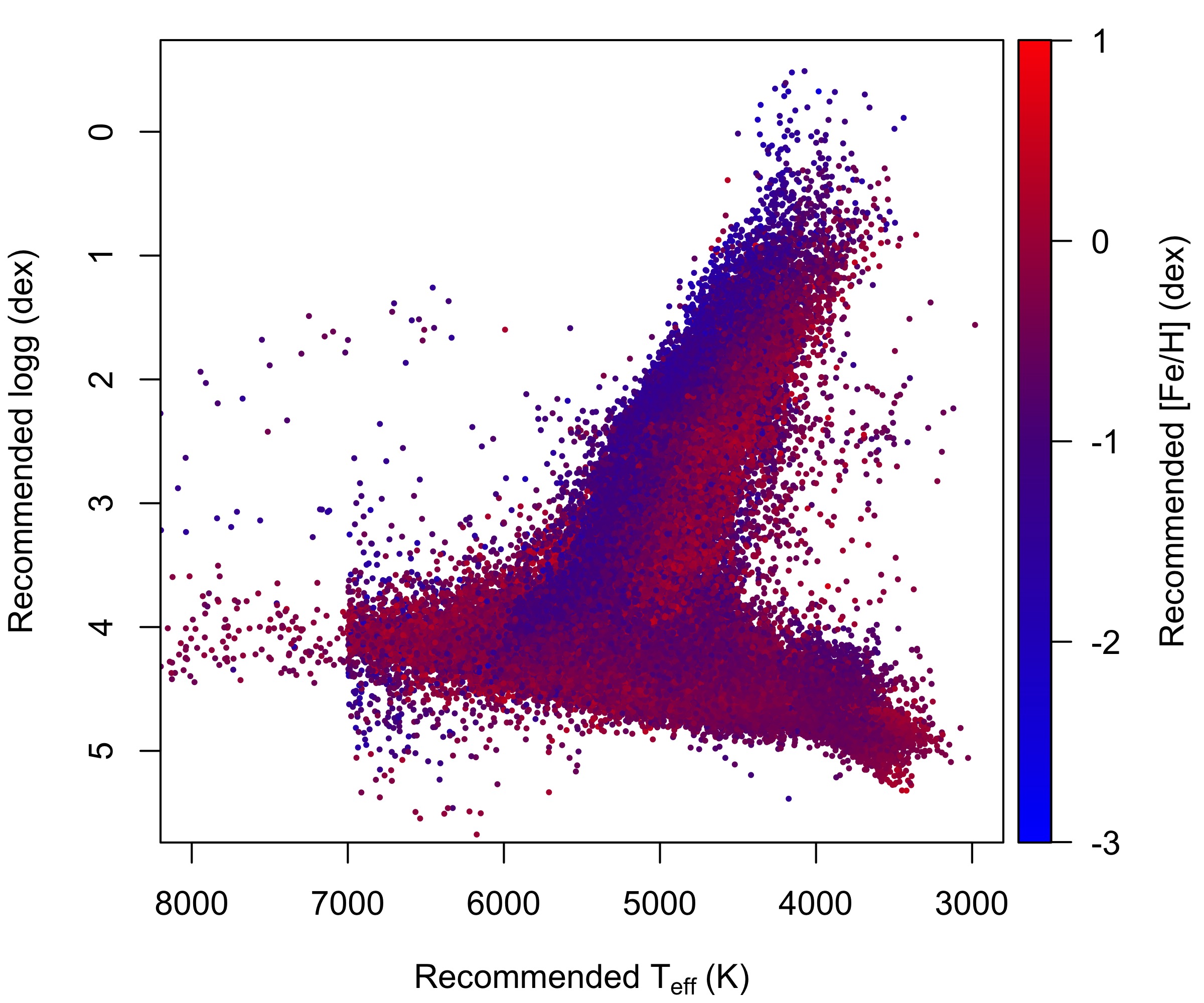
Figure 8: The final set of recommended parameters for the clean sample. Only stars having also an [Fe/H] estimate are shown. A long tail of hot stars and the WD sequence are not shown. See Section 4.5 for details.

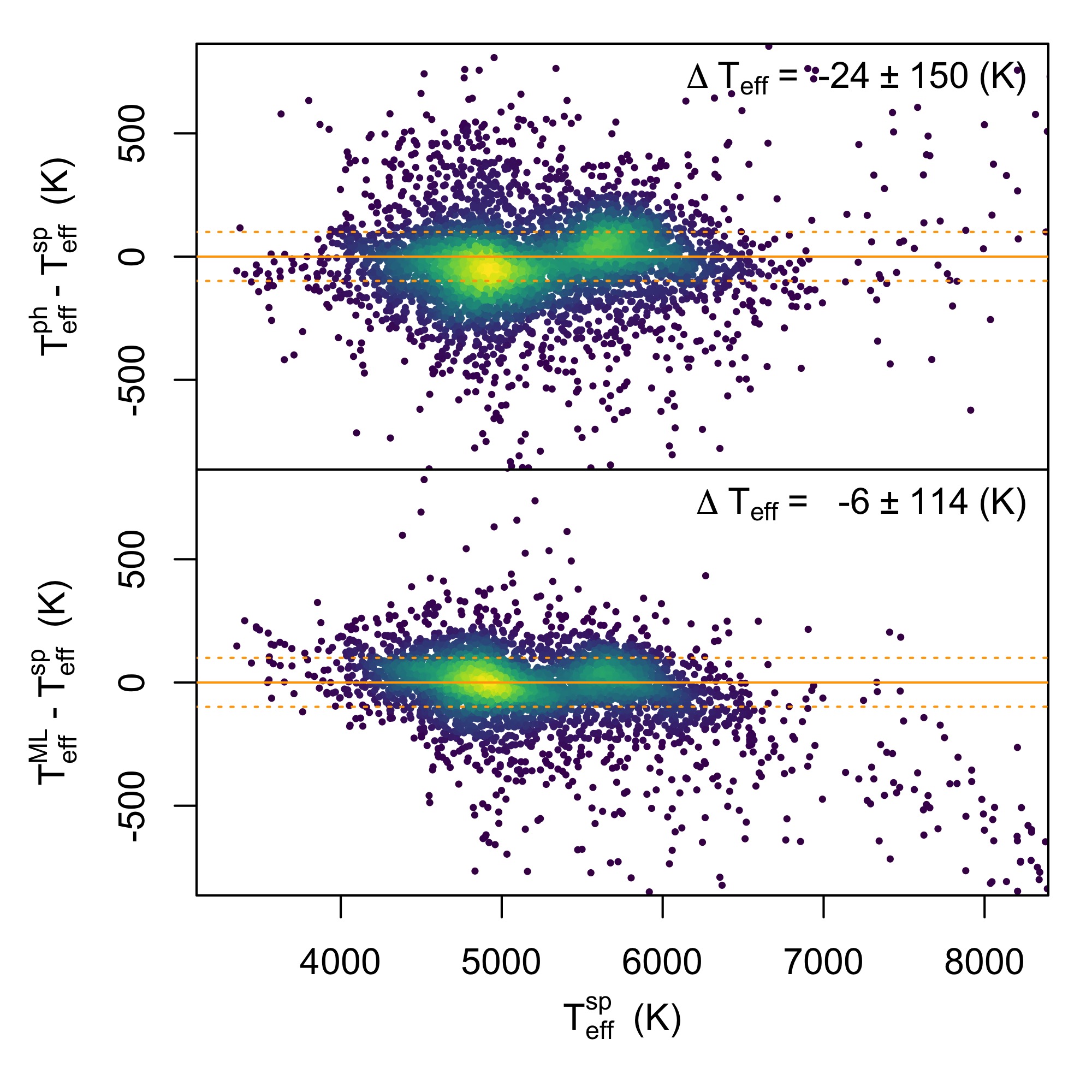
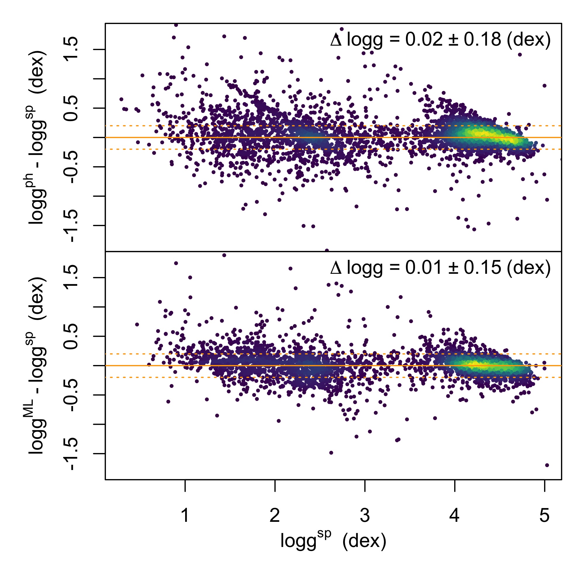
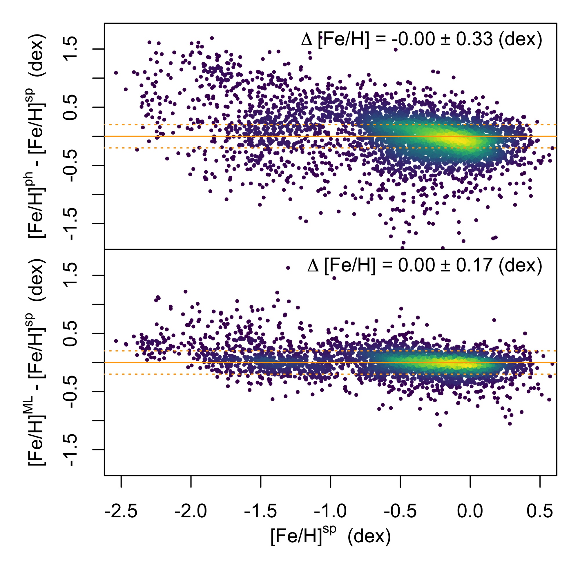
Figure 9: Comparison between parameters obtained with different methods. The top panels show the differences between the photometric and spectroscopic parameters, the bottom ones between the machine-learning and the spectroscopic ones. The left panels show the case of T_eff, the middle ones of log$g$, and the right ones of [Fe/H]. The median difference and MAD are written in each panel. The horizontal lines mark the zero (perfect agreement), $\pm$100 K (for T_eff), and $\pm$0.2 dex differences (for log$g$ and [Fe/H]), respectively. See Section 4.5 for more details.

4.5.1 Spectroscopic parameters and radial velocity

The first method we employed is based on spectroscopy. We used data from the SoS I (Tsantaki et al. 2022, see also Section 3.5), which contains homogenized, combined, and recalibrated RVs for about 11 million stars, with zero-point errors of a few hundred m/s and internal uncertainties in the range 0.5–1.5 km/s, depending on each star’s survey provenance. It is based on data from Gaia DR2 (Gaia Collaboration et al. 2018); APOGEE DR16 (Ahumada et al. 2020); RAVE DR6 (Steinmetz et al. 2020); GALAH DR2 (Buder et al. 2018); LAMOST DR5 (Zhao et al. 2012); and Gaia-ESO DR3 (Gilmore et al. 2012).

We found RV estimates for 9643 stars and stellar parameters for 6365 stars in the combined catalogue. Because only RVs are carefully re-calibrated in SoS I, to obtain the other stellar parameters for stars observed in more than one survey, we simply took the mean of the parameters presented in Table 8 by Tsantaki et al. (2022), which is adequate for our present purpose. We complemented the SoS spectroscopic parameters using the white dwarfs identified in the Kong & Luo (2021) or Fusillo et al. (2021) catalogues (see also Section 4.4). This way, we could find additional RV estimates for 35 WDs and stellar parameters for 161 WDs, that were specifically derived with the use of WD synthetic spectra by the authors, comparing them with LAMOST and APOGEE spectra, respectively. For the stars in common between the two studies, we simply took the average of their values, that compared well with each other.

4.5.2 Photometric parameters

As a second method, we used the accurate Landolt and Stetson photometry, together with our preliminary CMD classification, to compute photometric T_eff and log$g$ estimates. For the T_eff computation we used:

• for the FGK dwarfs and giants, we used (V-I)₀ which is the least sensitive to metallicity, and the relations by González Hernández & Bonifacio (2009) for dwarfs and giants;

• for stars resulting in T${}_{\rm{eff}}<4000$ K, we still used (V-I)₀, but we relied on the relation by Mann et al. (2015), which are computed specifically for cool stars;

• for stars hotter than 7000 K and 13000 K, we used the two relations by Deng et al. (2020), which however require (B–V)₀ rather than (V–I)₀;

• for white dwarfs, we fitted with a third-order polynomial the (B–V)₀ of the WDs having spectroscopic parameters from Kong & Luo (2021) or Fusillo et al. (2021) and we estimated a typical 15% uncertainty from the residuals of the fit; we then applied the relation to all stars classified as WDs either spectroscopically or from the CMD (i.e., with StarType WD or WD:, Section 4.4).

We further assigned T_eff to 4244 stars, using the Anders et al. (2022) catalogue, described in more details below. As can be seen from Figure 9, a good overall agreement is obtained between the spectroscopic and photometric temperatures, with a median difference of $\Delta$T_eff=–24$\pm$150 K, in the sense that the photometric temperatures are slightly smaller than the spectroscopic ones. For consistency, we corrected the photometric T_eff for this small offset. However, above $\simeq$7000 K, there are various large trends and substructures – mostly related to WDs and hot subdwarfs – and the uncertainties can be substantially higher than for cooler stars. We thus obtained photometric T_eff for 93% of the stars in the combined catalogue, i.e., the vast majority of the stars with distance and reddening estimates (Section 4.3), albeit with high uncertainties above $\simeq$7000 K.

To obtain log$g$ estimates, we computed bolometric corrections using the relations by Alonso et al. (1999), Flower (1996), and Mann et al. (2015), depending on the type of star and the validity range of the relations. With the bolometric luminosity, we estimated the radius from fundamental relations, and then log$g$ using the empirical logR$\sim$f(log$g$) relation by Moya et al. (2018), which is based on a sample of stars hotter than about 5000 K. For cooler stars, both dwarfs and giants, the log$g$ estimate is much more uncertain than for warmer stars. The photometric log$g$ obtained in this way have a median difference of $\Delta$log$g$=–0.2$\pm$0.4 dex with the spectroscopic log$g$, and they show a lot of substructure, especially below 5000 K. However, we found that the log$g$ estimates obtained by means of machine learning by Anders et al. (2022) from photometry and astrometry (see below for more details) are in better agreement with the spectroscopic parameters and show a much smoother behavior across the CMD, especially for K and M main sequence stars. We thus used the Anders et al. (2022) log$g$ estimates whenever available, and the above photometric ones for 21381 hot stars for which the Anders et al. (2022) estimates are not available. The comparison of the log$g$ estimates obtained by combining the two approaches yields $\Delta$log$g$=+0.02$\pm$0.18 dex, and we thus obtained photometric log$g$ estimates for 91% of the stars in the combined catalogue.

Finally, it is not possible to derive reliable estimates of [Fe/H] from simple relations based on Johnson-Kron-Cousins photometry. Thus, we used three different literature catalogues, in the following order or preference:

• The Xu et al. (2022) catalogue, which is based on LAMOST DR7 and Gaia EDR3 data, to provide photometric [Fe/H] estimates based on the stellar loci of stars with known metallicity; their [Fe/H] estimates show good agreement with the spectroscopic [Fe/H], with no significant trend and just a small bias: $\Delta$[Fe/H]=–0.07$\pm$0.35 dex; these were available for 24240 stars in our combined catalogue;

• The Anders et al. (2022) catalogue mentioned above, which results from the application of the machine-learning code StarHorse (Santiago et al. 2016; Queiroz et al. 2018) to the astrometry and the photometry from Gaia EDR3, and to the combined photometry from 2MASS (Skrutskie et al. 2006; Cutri et al. 2012), Pan-STARSS1 (Chambers et al. 2016; Flewelling 2016), Skymapper, and AllWISE (Cutri et al. 2013), matched using the same cross-matched algorithm used here (Marrese et al. 2017, 2019); these data show a clear trend when compared to the spectroscopic [Fe/H] (Section 4.5.1) where the metal-poor end at about [Fe/H]$\simeq$–2.0 dex is overestimated by about 0.5–1.0 dex, with a large scatter, while the metal-rich one at about [Fe/H]$\simeq$0.5 dex is underestimated by about 0.5 dex; we obtained photometric [Fe/H] estimates for 126706 stars, albeit less accurate than the Xu et al. (2022) ones;

• the [Fe/H] estimates by Miller (2015), based on SDSS 10 photometry (Ahn et al. 2014), which are available for 15523 stars in our combined catalogue; these estimates show a very similar trend with the spectroscopic [Fe/H] estimates as the Anders et al. (2022) ones, therefore, we used them for the 409 stars that did not have an estimate by Anders et al. (2022) or Xu et al. (2022);

• the [Fe/H] estimates by Chiti et al. (2021), based on SkyMapper photometry (Wolf et al. 2018), which are available for 998 stars in our combined catalogue; these saturate at about [Fe/H]$\simeq$–1.0 dex but are linearly correlated with the spectroscopic estimates below [Fe/H]$\simeq$–1.2 dex; we used them for 12 additional stars without an estimate by other sources.

The comparison between photometric and spectroscopic parameters is shown in the top panels of Figure 9.

4.5.3 Machine learning parameters

Having a sizeable set of stars with reliable spectroscopic parameters from the SoS, and keeping in mind the difficulties of obtaining log$g$ and [Fe/H] estimates for field stars from photometry (see Figure 9, top panels), we experimented with ML algorithms as well. It has indeed already been shown that purely numerical methods, such as ML techniques, can be successfully employed to estimate stellar parameters from photometric inputs (see the cited work by Miller 2015; Santiago et al. 2016; Queiroz et al. 2018; Xu et al. 2022; Anders et al. 2022, and references therein).

There is a large number of ML techniques in the literature that can apply to the case presented in this study. The problem at hand, in the ML lexicon, can be categorized as a supervised regression problem. Supervised ML methods are trained on a relatively small sample of objects, where the expected output is known (in our case, the spectroscopic T_eff, log$g$ or [Fe/H] from Section 4.5.1). Over this training sample, the algorithm learns how to transform the input variables, which can be an arbitrary number (see Table 6), into the output estimates by minimizing the resulting error. The trained algorithm is then tested on an independent sample, where the output is still known but is not provided to the algorithm, in order to prove that it can indeed work in a general case. The size of the sample used for both training and testing is crucial to maximize the performances of the method. We tested several ML methods, namely: Random Forest (RF Liaw & Wiener 2002), Probabilistic Random Forest (PRF Reis et al. 2019), K-Neighbours (KN Goldberger et al. 2005), Support Vector Regression (SVR Drucker et al. 1997), Multi-Layer-Perceptron (MLP Murtagh 1991). In the end we identified the SVR method to have the best results, outperforming the other methods by a considerable margin.

Table 6: Best photometric input variables selected for each ML stellar parameter estimation (T_eff, log$g$, and [Fe/H]) and for each quality level (gold, silver, bronze). We also indicate the sample size available for both the training and testing of the ML algorithm. See Section 4.5.3 for details.

Dataset	Parameter	Sample size	Input variables∗
Gold	Teff	2260	Dist, E(B–V), $\sigma$E(B–V), Uabs, Babs, Vabs, Rabs, Iabs, U, B, V, $\sigma$V, R, I, $\sigma$I, T${}_{\rm{eff}}^{\rm{photo}}$, [Fe/H]photo
	log$g$	2260	Dist, Uabs, Rabs, Iabs, U, B, V, R, I, T${}_{\rm{eff}}^{\rm{photo}}$, log$g^{\rm{photo}}$, [Fe/H]photo
	[Fe/H]	2366	Dist, E(B–V), Uabs, Babs, Vabs, Rabs, B, V, R, I, T${}_{\rm{eff}}^{\rm{photo}}$
Silver	(all)	3154	Dist, E(B–V), Uabs, Babs, Vabs, B, V, I, T${}_{\rm{eff}}^{\rm{photo}}$
Bronze	(all)	4290	Dist, E(B–V), Babs, Vabs, B, V, I, T${}_{\rm{eff}}^{\rm{photo}}$
∗The symbols Uabs, Babs, Vabs, Rabs, Iabs refer to the absolute and dereddened magnitudes; the ”photo” superscript to photometric parameters.

Table 7: Typical (median) error on the ML estimates of the parameters for each training dataset (gold, silver and bronze).

Dataset	Teff	log$g$	[Fe/H]
	(K)	(dex)	(dex)
Gold	98	0.14	0.14
Silver	137	0.16	0.20
Bronze	403	0.59	0.45

We initially identified a set of input values for the ML algorithms from the photometric variables present in the catalogue. ML methods cannot correctly treat empty (null or NaN) values, thus the major limiting factor on the size of the sample for training and testing (and on the final number of parametrized stars) is that some parameters, mostly R and U magnitudes, are frequently missing. By minimizing the error, i.e., the difference between the training parameters and the output ones in the test phase, we identified an optimal set of input variables, depending on the specific parameter that we are trying to estimate and that are indicated in Table 6. The estimates produced with these input parameters sets are labelled with starMethod=ml_gold in the catalogue (55231 stars). We also identified two reduced sets of input variables, which allow the method to be applied to additional sets of stars, although with reduced accuracy. These samples are labelled as (starMethod=ml_silver and ml_bronze) in the combined catalogue, amounting to 102959 and 1075 stars, respectively. In the case of silver parameters we essentially drop the R magnitude, while for the bronze ones we also drop the U magnitude.

After multiple trials, we selected the following operational strategy to estimate the parameters over the widest possible sample. Since the sample selection can influence the output of the algorithm, we decided to iterate the algorithm 100 times, each time randomly selecting half of the ML sample for training, and the other half for testing. Then, for each iteration, we applied the method to the whole sample of stars having all the relevant input variables. We selected as our best estimate for each star the median value of the 100 parameter estimates. We verified that the result is consistent with the best possible estimate using a single iteration and 100% of the ML sample for training. This approach permits to compute a Median Absolute Deviation (MAD) of the estimate for each star, which can be seen as the precision of the trained method in producing the same value independently of the sample selection. This also means that the method is self-consistent and reproducible within the MAD, and we can use it to filter out predictions with larger MAD values as inaccurate. For each parameter, we also computed the standard deviation of the previously defined best estimate on the ML sample by comparing with the spectroscopic parameters (Table 7, see also Figure 9). We finally computed the uncertainty on each parameter and for each star by taking the quadrature sum of the MAD (on each star) and the above standard deviation.

In Figure 9 (bottom panels) we show the error distribution obtained for each estimated variable obtained over the ML sample (as described before). We highlight that the [Fe/H] estimates obtained with SVR, differently from what observed in Anders et al. (2022) and Miller (2015), do not show such a large trend of overestimation for low metallicity and underestimation for high metallicity. Also, there is no saturation effect in the ML metallicity, as opposed to the estimates by Chiti et al. (2021). We believe that the main reason for the better performance obtained here lies mostly in the choice of the algorithm. In fact, when using a Random Forest insted of the SVR, we found the same trend as Anders et al. (2022) and Miller (2015) with the spectroscopic metallicity. Other factors that may have also helped are the choice of a large and diverse set of input parameters (see Table 6) and the fact that we used a reliable and large sample of spectroscopic parameter estimates for the training of the algorithm, covering the relevant parameter space. We believe it will be worth investigating the matter further and trying to apply our method to larger photometric samples such as the SDSS or Pan-STARRS in the near future.

Finally, we filtered out the following samples:

• white dwarfs estimates are particularly unrealistic in all parameters ($\simeq$ 800 stars);

• some of the [Fe/H] results outside of the range covered by the training sample (–3 to +1 dex), and with a MAD greater than 0.9 dex ($\simeq$3000 stars);

• most of the log$g$ results below –0.5 dex, which had MAD higher than 0.9 dex ($\simeq$1600 stars);

• T_eff for stars with (V–I)${}_{0}<-0.23$ mag, which appear to be too cool by hundreds or thousands of degrees, perhaps due to an under-representation of the category in the ML sample ($\simeq$300 stars).

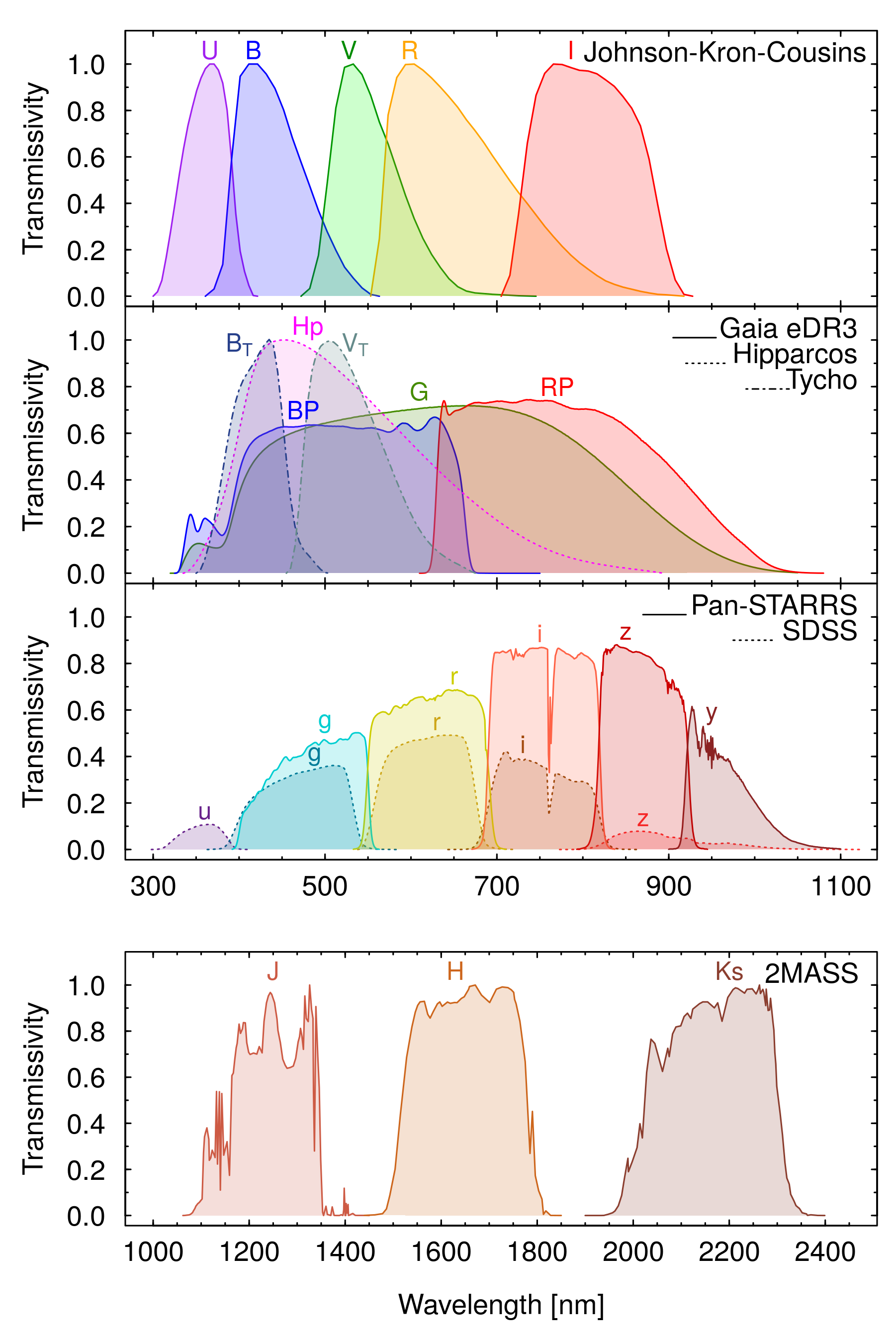
Figure 10: Summary of the photometric systems used to compute color transformations with the Johnson-Kron-Cousins system. The passbands were obtained from the SVO Filter Profile Service (see Section 5 for more details).

5 Relations with other photometric systems

To obtain transformations between the Johnson-Kron-Cousins system and some of the currently most used photometric systems, we looked for the counterparts of our clean sample standards (Section 4.1) in the large photometric surveys that use those photometric systems. To this aim, we used the official cross-matches of Gaia ERD3 with large photometric surveys, publicly available at the SSDC Gaia portal or the Gaia archive, which were obtained with the same cross-match algorithm used here (Marrese et al. 2017, 2019). Moreover, we only selected stars with a relatively low reddening, E(B–V)$\lesssim$0.3–0.8 mag, depending on the exact color combination and the direction of the reddening vector in that plane. The final catalogue of the magnitudes of the Landolt and Stetson standards in all the considered photometric systems is presented in Table 8. More details about the sample selections can be found in the following sections. Figure 10 summarizes the photometric systems and passbands considered. The transmissivity curves used in the figure were obtained from the SVO Filter Profile Service (Rodrigo et al. 2012; Rodrigo & Solano 2020). In particular, we used the passbands by Bessell & Murphy (2012), Riello et al. (2021), Moro & Munari (2000), Tonry et al. (2012), Doi et al. (2010), and Cohen et al. (2003).

For each photometric system, we computed the transformations as polynomial fits in the form:

$$Y=\Sigma_{i}\leavevmode\nobreak\ a_{i}\leavevmode\nobreak\ X^{i}$$ (1)

where $Y$ is a difference between two magnitudes in the two systems (e.g., G–V or B–G) and $X$ is a color in one of the two systems (e.g., B–V or G_BP–G_BP). The choice of the order of the polynomial was made by inspecting the residual plots and by selecting the lowest polynomial order that removes any residual systematic oscillations (wavy patterns) in the residuals, or that reduces it below the overall spread in the residuals. Although the data are often of very high quality, there are sometimes substructures, jumps, or secondary branches. These arise naturally because of: (i) the magnitude dependent uncertainties and (ii) the different sensitivity of the employed photometric passbands to different spectral features. Rather than using a weighted fit, which would bias the fits in favour of bright stars, we opted for a smoothing of the Y vector before fitting. We replaced each Y value with the median of the three closest values after sorting in $X$, iteratively for three times (Beyer 1977). This minimizes any outlying features caused by higher reddening stars or specific minority stellar sub-groups (such as WDs or SDs), and it also has the side advantage of slightly improving the fits at the borders, where there are statistically much fewer stars. The disadvantage is that minority components (e.g., WDs or SDs) can be in some cases not well represented by the fits. The coefficients of all the 167 polynomial fits are presented in Table 9. More details on the fitting procedure, adopted choices, and goodness of the fits can be found in the following sections.

With the data presented in Table 8, it is possible to compute additional color transformations between the explored samples in color combinations that we did not include in Table 9. Using the data in Table 5, it should also be relatively easy to identify Landolt and Stetson standards in any other survey or catalogue, if they are present. This will enable the computation of transformations to and from additional photometric systems not considered in this work. Finally, we have used mostly giants and dwarfs, so in several cases our transformations do not apply to WDs, YSO, or hot subdwarfs. However, with the classification provided in Table 5 and the magnitudes in Table 8, users can derive their own specific transformations for these and other less represented stellar types.

Table 8: Magnitudes of stars in the combined catalogue (Table 5) in the different photometric systems considered in Section 5. Only stars with a Gaia EDR3 match, belonging to the clean sample (Section 4.1), and with a match in at least one of the photometric surveys, after survey-specific quality cuts, are included (see Sections 5.1–5.5 for details).

Column	Units	Description
ID		Star ID from Table 5
Gaia EDR3 ID		Gaia Source ID from EDR3
G′	(mag)	Corrected Gaia G magnitude
$\delta$G′	(mag)	Recomputed error on G′
G${}_{\rm{BP}}^{\prime}$	(mag)	Corrected Gaia GBP magnitude
$\delta$G${}_{\rm{BP}}^{\prime}$	(mag)	Recomputed error on G${}_{\rm{BP}}^{\prime}$
G${}_{\rm{RP}}^{\prime}$	(mag)	Corrected Gaia GRP
$\delta$G${}_{\rm{RP}}^{\prime}$	(mag)	Recomputed error on G${}_{\rm{RP}}^{\prime}$
HIP ID		HIPPARCOS identifier
HP	(mag)	Hipparcos magnitude
$\delta$HP	(mag)	Error on HP
TYC ID		Tycho identifier
BT	(mag)	Tycho B magnitude
$\delta$BT	(mag)	Error on BT
VT	(mag)	Tycho V magnitude
$\delta$VT	(mag)	Error on VT
SDSS ID		SDSS DR13 identifier
uSDSS	(mag)	u PSF magnitude in SDSS  DR13
$\delta$uSDSS	(mag)	Error on uSDSS
gSDSS	(mag)	g PSF magnitude in SDSS  DR13
$\delta$gSDSS	(mag)	Error on gSDSS
rSDSS	(mag)	r PSF magnitude in SDSS  DR13
$\delta$rSDSS	(mag)	Error on rSDSS
iSDSS	(mag)	i PSF magnitude in SDSS  DR13
$\delta$iSDSS	(mag)	Error on iSDSS
zSDSS	(mag)	z PSF magnitude in SDSS  DR13
$\delta$zSDSS	(mag)	Error on zSDSS
PS1 ID		Pan-STARRS-1 identifier
gPS	(mag)	g PSF magnitude in PS1
$\delta$gPS	(mag)	Error on gPS
rPS	(mag)	r PSF magnitude in PS1
$\delta$rPS	(mag)	Error on rPS
iPS	(mag)	i PSF magnitude in PS1
$\delta$iPS	(mag)	Error on iPS
zPS	(mag)	z PSF magnitude in PS1
$\delta$zPS	(mag)	Error on zPS
yPS	(mag)	y PSF magnitude in PS1
$\delta$yPS	(mag)	Error on yPS
2MASS ID		2MASS PSC identifier
J2MASS	(mag)	J magnitude from 2MASS PSC
$\delta$J2MASS	(mag)	Error on J2MASS
H2MASS	(mag)	H magnitude from 2MASS PSC
$\delta$H2MASS	(mag)	Error on H2MASS
K2MASS	(mag)	Ks magnitude from 2MASS PSC
$\delta$K2MASS	(mag)	Error on K2MASS

Table 9: Coefficients of the polynomial fits (Equation 1) to convert magnitudes between the Johnson-Kron-Cousins photometric system and literature photometric systems of various photometric surveys, based on the data in Table 8. See Section 5 for more details.

Column	Units	Description
Survey		Provenance of the survey data
		(example: Gaia EDR3, SDSS DR13, …)
System		Photometric system of the survey data
		(example: Gaia, ugriz, JHK, …)
X	(mag)	Input color (examples: V–I or GBP–GRP)
Xmin	(mag)	Lower validity limit for the fit
Xmax	(mag)	Upper validity limit for the fit
Y	(mag)	Output color (examples: G–V or g–V)
$a_{0}$		Coefficient of zero-order term
$a_{1}$		Coefficient of first-order term (X)
$a_{2}$		Coefficient of second-order term (X2)
…		(i.e., one column for each coefficient)
$a_{n}$		Coefficient of nth-order term (Xn)
$\sigma$	(mag)	Standard deviation of Y residuals
N		Number of stars used in the fit
Validity		Notes on validity regime
		(examples: giants, dwarfs, all)
Notes		Additional cautionary notes
		(example: not for WDs)

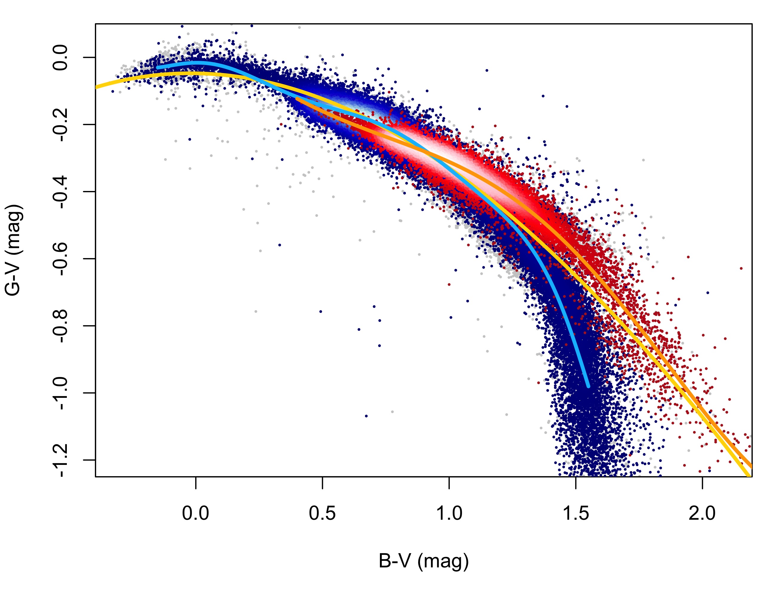
Figure 11: Example of transformation from V, B–V to the Gaia G magnitude, illustrating the advantage of performing separate polynomial fits for dwarfs and giants. The whole clean sample is plotted in the background as grey dots, dwarfs are plotted in blue, and giants in red. The polynomials fitted on the two samples separately are plotted as a light blue and an orange line, respectively. The polynomial fit by Riello et al. (2021) is plotted in yellow: it reproduces the dwarfs at blue colors, the giants at red colors, and passes between the two at intermediate colors.

5.1 The Gaia EDR3 system

Before computing the transformations between the Johnson-Kron-Cousins and the Gaia EDR3 photometric system (Figure 10), we corrected for some known effects in the Gaia EDR3 photometry. This has to be taken into consideration when using our transformations on the publicly available Gaia EDR3 magnitudes. In particular:

• saturated stars were corrected following the equations C.1, C.2, and C.3 in Appendix C by Riello et al. (2021); although the impact of saturation has decreased with respect to Gaia DR2 (Rowell et al. 2021), a small correction is still needed;

• the G magnitude of stars with a six-parameter solution, i.e., for which the BP and RP magnitudes where not available to produce the astrometry and, most importantly the PSF/LSF calibration (Rowell et al. 2021), were corrected following the recipe in Section 8.3 and Table 5 by Riello et al. (2021);

• the G magnitudes of bright blue giants (8$<$G$<$13 mag and G_BP–G_RP$<$–0.1 mag) has been corrected following the recipe in Section 8.4 by Riello et al. (2021); the linear trend with G is probably caused by small problems in the PSF/LSF calibration (Rowell et al. 2021).

The $a_{i}$ coefficients for 35 different Gaia and Johnson-Kron-Cousins color combinations are provided in Table 9, along with their color validity ranges, the standard deviation of the $Y$ residuals of each fit, and relevant annotations. An example is presented in Figure 11, where a comparison with the transformations by Riello et al. (2021) is also presented. Outside of the indicated color validity ranges, the transformations are either less accurate or completely unreliable, depending on the polynomial behavior at the borders, and therefore caution is required. In particular, we noted that in most of the relations reported in Table 9, it was necessary to perform separate fits for dwarf and giant stars. The largest differences are observed for M stars, as already noted by Riello et al. (2021), but in most cases dwarfs and giants occupy different loci at all colors, not just at the reddest ones, as illustrated in Figure 11. We separated giants and dwarfs using both our stellar classification (Section 4.4) and parametrization (Section 4.5). In particular, we separated the samples at log$g$=3.5 dex and we further removed stars with log$g$$>$5.5 dex from the dwarfs sample (except for those cases in which the WDs and SDs could be well fitted together with the dwarfs). We also note that, to improve the fits, we removed highly reddened stars, therefore our transformations are in general not appropriate for stars with reddening E(B–V)$\gtrsim$0.5 mag.

The WDs and hot sub-dwarfs did not follow the same relations as the normal dwarfs and giants in some of the fits. When this occurred, we noted it down in the Notes column of Table 9. Additionally, some transformations involving the U band, which is not well covered by the Gaia passbands, require a very high order and provide large spreads (3% or more); some others have a non monotonic behaviour. In some of these cases, we still provided the coefficients, but inserted a warning in the Notes column. Finally, while the standard U band can be generally used to predict Gaia photometry, the opposite is not true, because a simple polynomial cannot be used to reproduce the complex behaviour in these planes with the G_BP–G_RP color and magnitude differences involving the U band.

5.2 The Hipparcos and Tycho systems

The Hipparcos astrometric satellite (Perryman et al. 1997; Hoeg et al. 1997; van Leeuwen 2007), the predecessor of Gaia, provided photometry in one very wide, white-light band labelled H_P. The photometric system has been discussed in detail by Bessell (2000). The Tycho instrument onboard also provided color information, by means of a blue and a red wide band, B_T and V_T, respectively (Figure 10). We used the cross-match between Gaia EDR3 (Marrese et al. 2017, 2019) with the re-reduction of the original Hipparcos data (van Leeuwen 2007) and the Tycho-2 re-analysis of the Tycho data (Høg et al. 2000). We found 76 stars in common with the Hipparcos and 1315 with the Tycho catalogue.

Given the small sample sizes and the large uncertainties in the B_T and V_T magnitudes, the spreads on the computed relations, especially those involving the B_T and V_T bands, are often of 10–20%, reaching above 30% when involving the U band. The two transformations involving only H_P have instead spreads of the order of 2–3%. We did not perform separate fits for dwarfs and giants. We computed 10 relations between H_P and the $UBVRI$ magnitudes, using the smaller sample of Hipparcos stars with simultaneous estimates of H_P, B_T, and V_T (these transformations are labeled ”Hipparcos 2007” in Table 9). We also computed 10 relations between the $UBVRI$ and the B_T, and V_T bands, using the larger sample of Tycho-2 stars (these are labelled ”Tycho-2” in Table 9), where we selected only stars with $\delta$B_T and $\delta$V_T smaller than 0.1 mag for the fits, remaining with 24 stars from Hipparcos and 786 for Tycho. The polynomial orders of these fits are considerably lower than in other systems, between 2 and 3.

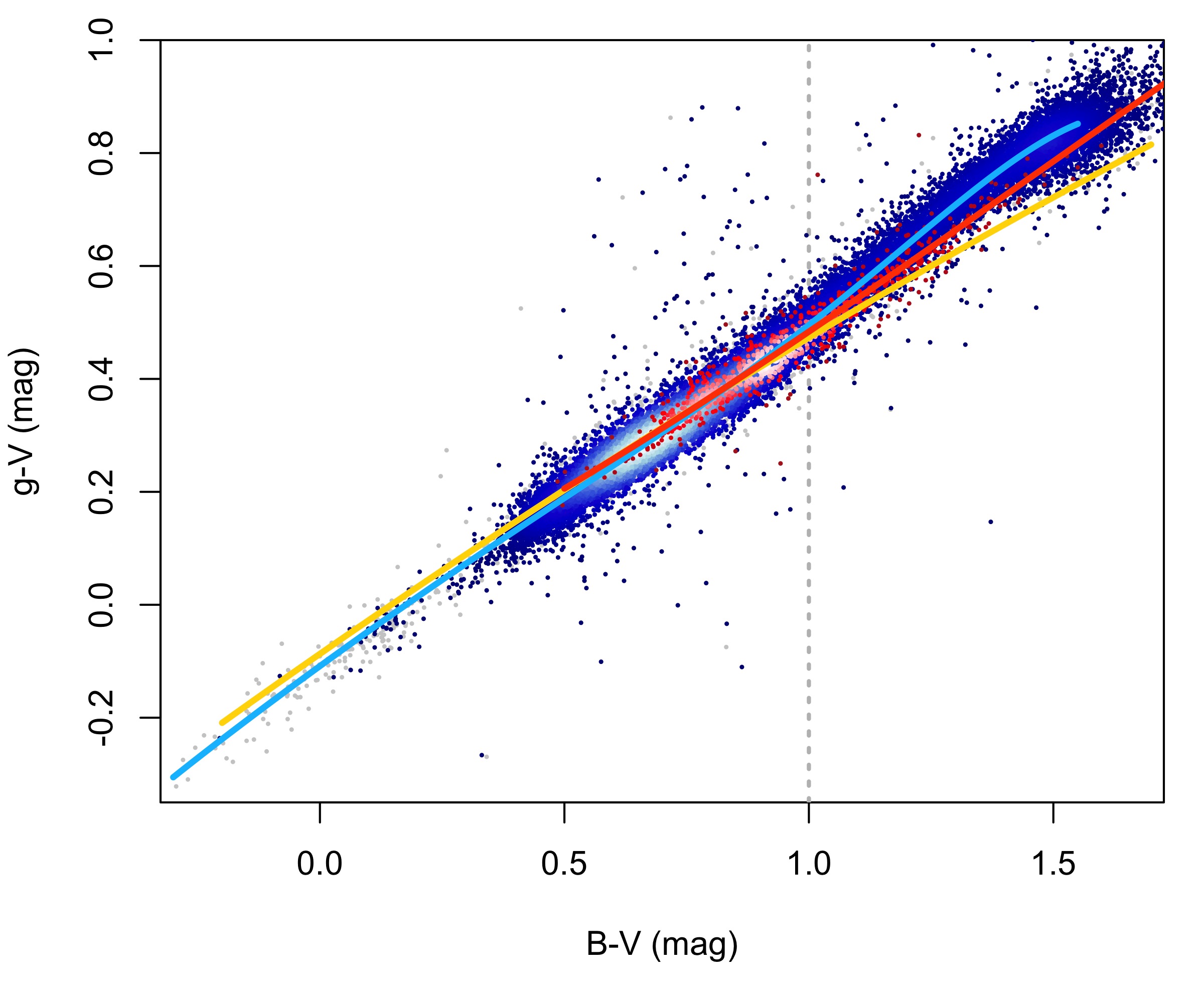
Figure 12: Similar to Figure 11, but for the SDSS DR13 ugriz system. In particular, the B–V, g–V case is shown. The clean sample is plotted in the background as grey dots, dwarfs are plotted in blue, and giants in red. The polynomials fitted on the two samples separately are plotted as a light blue and an orange line, respectively. The original transformation by Rodgers et al. (2006), who used the Smith et al. (2002) ugriz standards and who could only count on four stars redder than B–V=1 mag (grey dotted line), is shown in yellow. For B–V$<$1 mag, the three relations agree within about 2%. In general, the Rodgers et al. (2006) relation agrees more with the giants sample than with the dwarfs one.

5.3 The SDSS DR13 ugriz system

The ugriz photometric system was first defined by Fukugita et al. (1996) and Newberg et al. (1999) and it is the system of choice to derive photometric redshifts of (faint) external galaxies for cosmological studies, thanks to its very wide and equally spaced passbands (Figure 10), thus it does not focus on specific stellar features (Bessell 2005). Initially, the passbands were indicated in the literature with apices (u^′g^′r^′i^′z^′), to discern them from those of the older Thuan & Gunn (1976) system, which had narrower bands and no z filter. We will not use apices in the following. The standard stars in the ugriz system were provided by Smith et al. (2002) and the tranformations with the Johnson-Kron-Cousins system were provided by Rodgers et al. (2006). It is worth mentioning here that the Vera Rubin telescope (previously known as LSST, Ivezić et al. 2019) will instead employ a photometric system similar to the SDSS ugriz and Pan-STARRS grizy ones, but slightly different from both in the passband shapes. Additionally, APASS (Henden et al. 2012; Levine 2017), which is widely used by the community studying variable stars, uses the SDSS griz filters in combination with the Johnson-Kron-Cousins BV bands.

To derive new transformations using our standard catalogue, we used the publicly available Gaia EDR3 cross-match (Marrese et al. 2017, 2019) with SDSS DR13 (Albareti et al. 2017). In that release, a complete re-assessment of the SDSS half-billion object photometry was performed, including improvements of the data processing and a full re-calibration of the ugriz magnitudes (Finkbeiner et al. 2016), based on the zero-points of the Pan-STARRS system by Schlafly et al. (2012). We used the SDSS clean flag to select high-quality measurements. We excluded all duplicates found by the cross-match and we removed all stars with more than one neighbor. We further removed stars with E(B–V)$\gtrsim$0.3–0.8 mag, depending on the case, and errors on the SDSS magnitudes above the 95% percentile, as a function of magnitude, in at least three bands. We remained with a sample of about $\simeq$38 000 stars out of the original $\simeq$63 000.

We used Equation 1 and computed 26 polynomial fits to obtain SDSS magnitudes from Johnson-Kron-Cousins ones and vice versa. We restricted the relations to bands covering similar wavelength ranges (Figure 10) and therefore we could often use polynomials of lower order, especially for giants. Similarly to the previous cases, we found that it is often more effective to perform separate fits for dwarfs and giants. This occurrence is noted down in the Validity column of Table 9. Additionally, transformations involving the blue bands are generally not appropriate for cool stars and those obtained from red bands are less accurate for the hot stars. The transformations are also not appropriate for highly reddened stars, or for WD and hot sub-dwarfs in general.

An example of polynomial fit for the SDSS ugriz system is shown in Figure 12, where we also compare with the original transformations from Rodgers et al. (2006). It is important to note that the Rodgers et al. (2006) transformations were based on the Smith et al. (2002) standards and that only four stars were present in that sample with colors redder than B-V=1 mag. For this reason, their relation and ours diverge for redder stars in Figure 12. However, the agreement for B–V$<$1 mag is $\leq$2%.

5.4 The Pan-STARSS-1 grizy system

The Panoramic Survey Telescope and Rapid Response System (Pan-STARRS, Chambers et al. 2016; Flewelling 2016) photometric system (Tonry et al. 2012; Magnier et al. 2020) is similar to the ugriz one adopted by SDSS, but it does not have u and it adds a redder y band. At the same time, the passband shapes are slightly different from the SDSS ones (see Figure 10) and small differences are also expected with the upcoming Vera Rubin telescope passbands (Ivezić et al. 2019).

Similarly to the other surveys, we used the official Gaia cross-match (Marrese et al. 2017, 2019) to look for stars in common with our sample. For the reference photometry, we used the pre-filtered version of the PS1 release available in the Gaia archive, where data with only one detection, with large or null uncertainties or magnitudes, and with large errors on the coordinates were removed. We further removed stars with more than one neighbor or mate. This provided us with a starting clean sample of about 88 000 stars in common with our combined catalogue. Similarly to the case of the SDSS in the previous section, we computed 22 transformations, using the closest passbands in wavelength, therefore we did not need to use often high-degree polynomials. We also separated the giants from the dwarfs in most cases, and the WDs generally were well reproduced by the transformations appropriated for the dwarfs, unlike in the case of SDSS.

5.5 The 2MASS JHK system

The 2MASS survey (Two-Micron All Sky Survey Skrutskie et al. 2006; Cutri et al. 2012) is among the most used photometric survey in the near infrared wavelength range. Several authors provide transformations between optical photometric systems and the JHK system used in 2MASS. We believe that, because of the two very different wavelength regimes covered, these transformations have to be used with great caution, but we do understand that they can be helpful in a variety of applications. Here, we use the 2MASS PSC (Point Source Catalogue) of 470 million sources, which has been cross-matched with Gaia EDR3 using the same software used elsewhere in this paper (Marrese et al. 2017, 2019). We selected stars with no mates and no neighbours in the cross-match table, and we further imposed an angular distance smaller than 0.5”. We also made use of the various flags in the 2MASS PSC, to remove sources affected by blends, projected on extended sources, or with problems in the photometric data or processing. From a list of $\simeq$150 000 stars in common with our combined catalogue, we thus selected the best $\simeq$90 000.

We did not provide any transformations with the U-band, because of the large scatter around the fits ($>$0.5 mag) and the large dependency on metallicity. We found, in the U-band fits, color differences between solar metallicity and metal-poor stars reaching up to one magnitude, especially for giants. The dependency on metallicity is present also in other bands, mostly when involving the B, R, or H bands. Unfortunately, for the dwarfs sample, we could not count on enough good metallicity estimates, thus our fits for dwarfs are only valid for stars with [Fe/H]$\gtrsim$–1.0 dex. For giants, we sometimes split the sample at [Fe/H]=–0.8 dex and performed separate fits for the two groups, as appropriate and as annotated in the Validity column of Table 9. We computed in total 63 transformations with the 2MASS JHK system. In general, the transformations to obtain Johnson-Kron-Cousins magnitudes from 2MASS ones have large spreads, around 0.3–0.4, 0.2–0.3, 0.1–0.2 and 0.1 mag for B, V, R, and I respectively. The transformations to get 2MASS magnitudes from Johnson-Kron-Cousins ones have generally lower spreads, ranging from 0.03 mags to 0.1 mags.

An additional complication is that the different wavelength range covered (optical vs. infrared) implies a large amount of substructures in the color plots, revealing important differences in the underlying spectral energy distribution of the stars. For example, several bifurcations are evident in certain color combinations, which split stars according to their reddening (even if we remained below E(B–V)$\simeq$0.5 mag), to their gravity, separating giants from subgiants, and to their metallicity. Following all of these bifurcations would have multiplied the number of transformations that we had to provide, so we generally discarded the minority branches and provided the relevant information in the notes in Table 9. However, the potential – in terms of stellar classification power – of a combined optical-infrared photometry is enormous and is definitely worth exploring further.

6 Conclusions

We have provided a curated version of the widely used collections of secondary standards provided by Landolt and Stetson and their collaborators. We have selected stars with comparatively higher photometric accuracy and we profited from Gaia EDR3 data and literature catalogues to flag confirmed or suspected blends, binaries, and variable stars. We also classified and characterized stars making a wide use of the available literature data and of the exquisite Gaia data, in terms of evolutionary stage, stellar types, atmospheric parameters, reddening, distance, and radial velocity. In particular, we used the SVR regression algorithm, trained on the SoS spectroscopic data (Tsantaki et al. 2022) to derive machine learning parameters from the Landolt and Stetson photometry, which provides significantly better results compared to similar machine learning studies in the literature, especially as far as log$g$ and [Fe/H] determinations are concerned. We used the Gaia cross-match algorithm to identify the high-quality sample of Landolt and Stetson secondary standards in external surveys (Gaia, Hipparchos and Tycho, SDSS, Pan-STARRS-1, and 2MASS) and computed 167 transformations between those photometric systems and the Johnson-Kron-Cousins one. All the data presented in the paper tables are available electronically, on the CDS Vizier catalogue service and on the Gaia Portal at SSDC (http://gaiaportal.ssdc.asi.it/).