Probabilistic Predictability of Stochastic Dynamical Systems:
Metric, Optimality and Application

Abstract

To assess the quality of a probabilistic prediction for stochastic dynamical systems (SDSs), scoring rules assign a numerical score based on the predictive distribution and the measured state. In this paper, we propose an $\epsilon$-logarithm score that generalizes the celebrated logarithm score by considering a neighborhood with radius $\epsilon$. To begin with, we prove that the $\epsilon$-logarithm score is proper (the expected score is optimized when the predictive distribution meets the ground truth) based on discrete approximations. Then, we characterize the probabilistic predictability of an SDS by the optimal expected score and approximate it with an error of scale $\mathcal{O}(\epsilon)$. The approximation quantitatively shows how the system predictability is jointly determined by the neighborhood radius, the differential entropies of process noises, and the system dimension. In addition to the expected score, we also analyze the asymptotic behaviors of the score on individual trajectories. Specifically, we prove that the score on a trajectory will converge to the probabilistic predictability when the process noises are independent and identically distributed. Moreover, the convergence speed against the trajectory length $T$ is of scale $\mathcal{O}(T^{-\frac{1}{2}})$ in the sense of probability. Finally, we apply the predictability analysis to design unpredictable SDSs. Numerical examples are given to elaborate the results.

, ,

1 Introduction

1.1 Background

Stochastic noises are inevitable in dynamical systems, thus resulting in prediction uncertainties for future state trajectories. A probabilistic predictor predicts the target by a distribution rather than a single point, which can inherently quantify the prediction uncertainties. Therefore, probabilistic prediction for stochastic dynamical systems (SDSs) has attracted a surge of recent attention [2].

To measure the quality of a probabilistic prediction, scoring rules assign a numerical score based on the predictive distribution and the realized outcome [3, 4]. A scoring rule is called proper if the expected score can be maximized when the predictive distribution equals the ground truth, and it has a wide range of applications in statistical decision theory [5] and meteorology [6]. The fundamental idea of a proper score is to motivate a probabilistic predictor to be unbiased in predicting the true distribution. Practically, it can be used to compare the performance of different probabilistic predictors and to further improve them. One of the most celebrated proper scoring rules is the logarithm score, which assigns the score by the logarithm value of a probabilistic density function (PDF) at the outcome.

However, the logarithm score risks assigning reasonable scores for multimodal PDFs, mainly because a PDF being large at a point does not necessarily indicate a large probability around that point. Consider a multimodal PDF with a large value at point $a$ but quickly declines to 0 around its neighborhood. It also has a smaller value at another point $b$ but keeps invariant around its neighborhood. The logarithm score still assigns a larger score at $a$ than $b$, which is not reasonable for this type of PDFs.

1.2 Motivations

In the scenarios of SDS prediction, it is quite common for the predictive distributions to be multimodal (e.g., particle filters [7]), thus the logarithm score is not the most appropriate choice. By taking into account the neighborhood with tunable radius $\epsilon$, we propose an $\epsilon$-logarithm score in this paper, which can also degenerate into the traditional logarithm score by letting $\epsilon$ equal $0$. For this new scoring rule, we should first verify that it is indeed proper before applying it to characterize the trajectory prediction of SDSs.

A popular line of research is to design algorithms to probabilistically predict the state trajectories of SDSs, aiming for feasibility guarantee [8], better robustness [9], higher accuracy [10], etc. It may greatly boost the efficiency of designing predictors if we have a deeper understanding of the predictability of an SDS, e.g., what system features directly affect the value of predictability and which one possesses the largest weight. Under a proper scoring rule, the probabilistic predictability of an SDS can be naturally characterized by the optimal expected score.

Although the expected score is theoretically appealing in characterizing the system’s predictability, practically evaluating its value requires a sufficient amount of repeated samples for averaging. However, the samples generated from a typical SDS prediction scenario are usually temporal (a trajectory of states) rather than spatial (repeated samplings for the state at a fixed time step). While the average of spatial score samplings converges to the expectation as ensured by the law of large numbers, there is no simple guarantee for the average of temporal score samplings. Given any single trajectory generated from an SDS, under what condition can the temporal averaged score converge? Will it converge to the probabilistic predictability? How fast the convergence can be? These questions are answered in the following sections.

1.3 Contributions

The differences between this paper and its conference version [1] include i) the SDSs under consideration do not necessarily require i.i.d process noises; ii) the prediction problem has been reformulated under the general probabilistic prediction framework, and the performance metric under consideration also pivots from error metric to scoring rules; iii) the definition, evaluation and approximation of the predictability of SDSs are also adapted to the probabilistic predictors; iv) application of the predictability analysis is provided, based on which we design unpredictable SDSs and v) extended simulations are provided. The main contributions are summarized as follows.

• (Metric) We propose an $\epsilon$-logarithm score that generalizes the celebrated logarithm score by considering a neighborhood with radius $\epsilon$. When $\epsilon$ equals $0$, the proposed score will degenerate to the logarithm score. We also prove that it is a proper scoring rule based on a discrete approximation method. Benefiting from the neighborhood mechanism, the proposed score can provide more reasonable assessments for multimodal predictive distributions, which happen a lot in the prediction scenarios for SDSs.

• (Optimality) We characterize the probabilistic predictability of an SDS by the optimal expected $\epsilon$-logarithm score, regardless of specific prediction algorithms. Then, we approximate the probabilistic predictability with an error of the scale $\mathcal{O}(\epsilon)$. This approximation quantitatively strengthens our understanding of how a system’s predictability is jointly determined by the neighborhood radius, the differential entropies of process noises and the state dimension.

• (Convergence) We analyze the asymptotic convergence behaviors of the proposed score on any single trajectory generated from an SDS. It is proved that the score will converge to the system’s predictability when the process noises are independent and identically distributed. Furthermore, the convergence speed against the trajectory length $T$ is guaranteed to be of scale $\mathcal{O}(T^{-\frac{1}{2}})$ in the sense of probability.

• (Application) We apply the analysis on probabilistic predictability to design unpredictable SDSs. Specifically, we optimize over the noise distribution space to minimize the optimal expected $\epsilon$-logarithm score under some reasonable constraints. We also prove that our unpredictable design generalizes the design in a closely related work [11] by limiting our results to the one-dimension SDSs.

The remainder of this paper is organized as follows. Section II reviews the related works. Sec. III gives preliminaries, defines the $\epsilon$-logarithm score and formulates the problems of interest. Sec. IV introduces the discrete approximation method to prove the proposed score is proper. In Sec. V, we characterize the system’s predictability by evaluating and approximating the optimal expected score, and the asymptotic behavior of the score is presented. As an application, Sec. VI applies the conclusions about predictability to design unpredictable SDSs. Simulations are shown in Sec. VII, followed by the concluding remarks in Sec. VIII.

2 Related Works

In this section, we provide a brief review of the extensive research on analyzing the predictability of dynamical systems from deterministic to stochastic systems.

A large amount of insightful works contribute to the predictability analysis of deterministic dynamical systems. Lorenz considered prediction performance as the growing rate of initial state uncertainty, then defined predictability as the asymptotic exponential growing rate of initial prediction error [12]. Motivated by this idea, some famous indexes such as Lyapunov exponent and Kolmogorov-Sinai entropy were proposed to characterize the predictability of dynamical systems, see a review of these indexes in [13]. These early predictability analyses have found wide applications in the climatology fields such as atmospheric modeling, weather and climate prediction [14, 15, 16]. However, these works do not take noises or state measurements into consideration, thus can not be directly applied to characterize the predictability of SDSs.

Research on the predictability analysis of discrete-state SDSs mainly bifurcates into two directions. A body of research treats the predictability of SDS from an information-theoretic perspective without first evaluating the prediction performance, thus a lot of entropy-based predictability metrics were proposed. The entropy of stochastic process is defined as the joint entropy in [17, 18], based on which optimal prediction performance analysis and unpredictable system designs were presented in [19, 20, 21]. Another line of research steer the complicated evaluation of prediction performance by approximation techniques. In [22], an upper bound of the accurate prediction probability is derived based on standard Fano’s inequality. This bound is applied to the study of large-scale urban vehicular mobility [23]. Concerning more prior knowledge during the prediction process, this method is further enriched in [24] and [25].

Research on the predictability analysis of continuous-state SDS is relatively less than the discrete ones. In the field of climate forecasting, the predictability of an SDS is defined as the distance between a predicted distribution and climatological distribution based on entropy, relative entropy and mutual information [26, 27, 28]. In the field of state estimation, some concern the predictability as the effect of model mismatch on the steady solution of the Kalman filter [29], some study the predictability by evaluating the worst-case mean square error prediction performance of the Kalman filter [30]. Recently, an unpredictable design of SDS was developed in [11], which formulated an optimization problem with $\epsilon$-accurate prediction probability as the objective.

However, existing works on predictability analysis of SDSs mainly serve for point predictions, and it remains open and challenging to analyze the predictability under a probabilistic prediction framework.

3 Preliminaries and Problem Formulation

3.1 Preliminaries and Notations

In this paper, we denote random variables in bold fonts to distinguish them from constant variables, e.g., $\mathbf{x}$ is a random variable with PDF $p_{\mathbf{x}}(\cdot)$. We also denote a sequence $\{(\cdot)_{k}\}_{k=1}^{T}$ by $(\cdot)_{1:T}$.

3.1.1 Entropy and KL-Divergence

The Shannon entropy of a discrete random variable $\mathbf{x}$ with alphabet $\mathcal{X}$ and PDF $p_{\mathbf{x}}(x)$ is,

$$\mathrm{H}_{\mathrm{s}}(\mathbf{x}):=-\sum_{x\in\mathcal{X}}p_{\mathbf{x}}(x)\log p_{\mathbf{x}}(x).$$

The differential entropy of a continuous random variable $\mathbf{x}$ with support $\mathcal{X}$ and PDF $p_{\mathbf{x}}(x)$ is,

$$\mathrm{H}_{\mathrm{d}}(\mathbf{x}):=-\int_{x\in\mathcal{X}}p_{\mathbf{x}}(x)\log p_{\mathbf{x}}(x)\mathrm{d}x.$$

The KL-divergence measures how much distant $\mathbf{x}_{2}$ diverges away from $\mathbf{x}_{1}$, i.e.,

$$D_{\mathcal{KL}}(\mathbf{x}_{1}||\mathbf{x}_{2})\!:=\!\left\{\!\begin{array}[]{ll}\sum\limits_{x\in\mathcal{X}}p_{\mathbf{x}_{1}}(x)\log\left(\frac{p_{\mathbf{x}_{1}}(x)}{p_{\mathbf{x}_{2}}(x)}\right)&\text{discrete},\\ \int\limits_{x\in\mathcal{X}}p_{\mathbf{x}_{1}}(x)\log\left(\frac{p_{\mathbf{x}_{1}}(x)}{p_{\mathbf{x}_{2}}(x)}\right)\mathrm{d}x&\text{continuous}.\end{array}\right.$$

3.1.2 Probabilistic Prediction and Proper Scoring Rules

The problem of probabilistic prediction can be generally formulated as follows. Suppose a random variable $\mathbf{x}$ takes value on $\mathcal{X}$ with distribution $p_{\mathbf{x}}$, a probabilistic predictor predicts it by a distribution $\hat{p}_{\mathbf{x}}\in\mathcal{P}$, where $\mathcal{P}$ is a family of distributions over $\mathcal{X}$. When the value of $\mathbf{x}$ is materialized as $x$, a scoring rule,

$$S(\hat{p}_{\mathbf{x}},x):\mathcal{P}\times\mathcal{X}\to\mathbb{R},$$ (1)

assigns a numerical score $S(\hat{p}_{\mathbf{x}},x)$ to measure the quality of the predictive distribution $\hat{p}_{\mathbf{x}}$ on the realized value $x$. The expected scoring rule of $S$, usually sharing the same operator but possessing different operands, is defined as

$$S(\hat{p}_{\mathbf{x}},p_{\mathbf{x}}):\mathcal{P}\times\mathcal{P} \to\mathbb{R}$$ (2)

$$(\hat{p}_{\mathbf{x}},p_{\mathbf{x}}) \mapsto\mathbb{E}_{x}S(\hat{p}_{\mathbf{x}},x)$$

A scoring rule $S$ is proper with respect to the prediction space $\mathcal{P}$ if

$$S(\hat{p}_{\mathbf{x}},p_{\mathbf{x}})\geq S(p_{\mathbf{x}},p_{\mathbf{x}})$$ (3)

holds for all $\hat{p}_{\mathbf{x}},p_{\mathbf{x}}\in\mathcal{P}$. It is strictly proper if and only if the equality of (3) holds when $\hat{p}_{\mathbf{x}}=p_{\mathbf{x}}$. It is termed a local scoring rule if the score depends on the predictive distribution $\hat{p}_{\mathbf{x}}$ only through its value, $\hat{p}_{\mathbf{x}}(x)$, at $x$. For example, the logarithm score,

$$\mathcal{L}(\hat{p}_{\mathbf{x}},x):=\log\hat{p}_{\mathbf{x}}(x),$$ (4)

is most celebrated for being essentially the only local proper scoring rule up to equivalence [31, 32, 33]. While the linear score,

$$\operatorname{LinS}(\hat{p}_{\mathbf{x}},x):=\hat{p}_{\mathbf{x}}(x),$$

is not a proper scoring rule, despite its intuitive appeal in both theory and practice [3].

3.2 System and Predictor Model

Consider a discrete-time stochastic dynamical system, denoted by $\Phi$,

$$\Phi:\mathbf{x}_{k+1}=f(\mathbf{x}_{k})+\mathbf{w}_{k},$$ (5)

where $\mathbf{x}_{k}\in\mathbb{R}^{d_{x}}$ is the system state, $f:\mathbb{R}^{d_{x}}\to\mathbb{R}^{d_{x}}$ is the dynamic function, and $\{\mathbf{w}_{k}\}_{k=1}^{\infty}$ are process noises which are not necessarily required to be independent and identically distributed (i.i.d).

A probabilistic predictor keeps observing the states of $\Phi$ and predicting the conditional distributions of future states based on its knowledge of the system model and previous observations. Specifically, at time step $k$, suppose the predicting target $\mathbf{x}_{k+1}$ is a random variable with values in $\mathcal{X}$. Let $\mathcal{P}$ be a family of distributions over $\mathcal{X}$, the predictor intends to predict the conditional distribution $p_{\mathbf{x}_{k+1}\mid\mathbf{x}_{1:k}}(\cdot\mid x_{1:k})$ by $\hat{p}_{\mathbf{x}_{k+1}\mid\mathbf{x}_{1:k}}(\cdot\mid x_{1:k})\in\mathcal{P}$. Later, after the value of $\mathbf{x}_{k+1}$ is revealed as $x_{k+1}$, the prediction performance will be evaluated by a score $S(\hat{p}_{\mathbf{x}_{k+1}\mid\mathbf{x}_{1:k}}(\cdot\mid x_{1:k}),x_{k+1})$, where $S(\cdot,\cdot):\mathcal{P}\times\mathcal{X}\to\mathbb{R}$ is a scoring rule for probabilistic predictions.

3.3 Problems in Interest

Although the logarithm score is theoretically appealing to many statistical decision problems, it ignores the neighborhood of the target to be predicted. By generalizing the logarithm score, we propose an $\epsilon$-logarithm score as follows.

Definition 1 ($\epsilon$-logarithm score).

Given a neighborhood radius $\epsilon\geq 0$, a random variable $\mathbf{x}$ to be probabilistically predicted, and a family of distributions $\mathcal{P}$, the $\epsilon$-logarithm score evaluates the quality of any distribution $\hat{p}_{\mathbf{x}}\in\mathcal{P}$ on a realized outcome $x$ by

$$\mathcal{L}_{\epsilon}(\hat{p}_{\mathbf{x}},x):=\left\{\begin{array}[]{lr}\log\hat{p}_{\mathbf{x}}(x)&\epsilon=0,\\ \log\int_{\|s-x\|_{\infty}\leq\epsilon}\hat{p}_{\mathbf{x}}(s)\mathrm{d}s&\epsilon>0,\end{array}\right.$$ (6)

and the expected $\epsilon$-logarithm score is denoted as

$$\mathcal{L}_{\epsilon}(\hat{p}_{\mathbf{x}},p_{\mathbf{x}}):=\mathbb{E}_{x}\,\mathcal{L}_{\epsilon}(\hat{p}_{\mathbf{x}},x).$$ (7)

When $\epsilon=0$, $\mathcal{L}_{0}$ is the classical logarithm score, therefore strictly proper and local. The problem is, are these properties retained for $\mathcal{L}_{\epsilon}$ with $\epsilon>0$?

Problem 1.

Prove that the $\epsilon$-logarithm score is proper.

While the $\epsilon$-logarithm score $\mathcal{L}_{\epsilon}(p_{\mathbf{x}},x)$ scores a one-step prediction, we can naturally extend this definition to the trajectory prediction of SDSs.

Definition 2 ($\epsilon$-logarithm score for SDSs).

Given a neighborhood radius $\epsilon\geq 0$, a state trajectory $x_{1:T}$ generated from an SDS $\Phi$ and a family of distributions $\mathcal{P}$, the $\epsilon$-logarithm score for a probabilistic predictor $\hat{p}$ on this trajectory is the average of one-step scores, i.e.,

$$\bar{\mathcal{L}}_{\epsilon}(\hat{p}_{\mathbf{x}_{1:T}},x_{1:T})\!:=\!\frac{1}{T}\!\sum_{k=1}^{T}\mathcal{L}_{\epsilon}\left(\hat{p}_{\mathbf{x}_{k}\mid\mathbf{x}_{1:k-1}}(\cdot\mid x_{1:k-1}),x_{k}\right),$$ (8)

where $\hat{p}_{\mathbf{x}_{k}\mid\mathbf{x}_{1:k-1}}\in\mathcal{P}$ for $k=1,\ldots,T$. Then, the expected $\epsilon$-logarithm score is denoted as

$$\bar{\mathcal{L}}_{\epsilon}(\hat{p}_{\mathbf{x}_{1:T}},p_{\mathbf{x}_{1:T}}):=\mathbb{E}_{x_{1:T}}\bar{\mathcal{L}}_{\epsilon}(\hat{p}_{\mathbf{x}_{1:T}},x_{1:T}).$$ (9)

Given a probabilistic predictor and an SDS, we are interested in evaluating the expected $\epsilon$-logarithm score. Based on the evaluation, we optimize over the predictive space $\mathcal{P}$ to obtain the optimal expected $\epsilon$-logarithm score. Since the optimal score does not depend on a predictor, it characterizes the probabilistic predictability of an SDS.

Problem 2.

Evaluate the expected $\epsilon$-logarithm score and characterize the probabilistic predictability of an SDS by optimizing the expected $\epsilon$-logarithm score.

Although the expected $\epsilon$-logarithm score is theoretically appealing, practically evaluating its value requires a sufficient amount of samples for averaging. However, the data generated from a typical SDS prediction scenario is usually a trajectory of states rather than repeated samplings for one state. Therefore, we are also interested in answering the following questions.

Problem 3.

Given any state trajectory $x_{1:\infty}$ generated from $\Phi$, does the $\epsilon$-logarithm score $\bar{\mathcal{L}}_{\epsilon}(\hat{p}_{\mathbf{x}_{1:T}},x_{1:T})$ converge as $T$ approaches infinity? If it does converge, will it converge to the probabilistic predictability of $\Phi$? How fast the convergence is?

4 Evaluation of $\epsilon$-Logarithm Score

Evaluation of $\epsilon$-logarithm score is the fundamentation of all the problems to be studied. However, for a general probabilistic distribution, explicit expressions may not exist for the interval integrations. To overcome this challenge, a discrete approximation method is utilized to transform $\mathcal{L}_{\epsilon}$ to an analyzing-friendly form. Based on this transformation, we can prove that both $\mathcal{L}_{\epsilon}$ and $\bar{\mathcal{L}}_{\epsilon}$ are indeed proper scoring rules.

4.1 Discrete Approximation

Definition 3 (Partition).

A partition of a set $\mathcal{X}$, denoted by $\Sigma$, is a set that divides $\mathcal{X}$ into $N\in\mathbb{N}$ disjoint subsets, i.e.,

$$\Sigma:=\left\{A_{1},\cdots,A_{N}~{}\Bigg{|}~{}\bigcup\limits_{i=1}^{N}A_{i}=\mathcal{X},A_{i}\cap A_{j}=\emptyset,~{}\forall i\neq j\right\}.$$

Based on the partition, the space $\mathcal{X}$ can be treated as a set of $N$ small regions, and any element in $\mathcal{X}$ belongs to exactly one region. This belonging relation can be conveniently characterized by a label function as follows.

Definition 4 (Label function induced from $\Sigma$).

The label function $\Theta_{\Sigma}(\cdot)$ assigns each element $x\in\mathcal{X}$ to the region where it belongs in $\Sigma$, i.e.,

$$\Theta_{\Sigma}(x):=\sum\limits_{i=1}^{N}i\cdot\mathbb{I}_{A_{i}}(x),$$

where $\mathbb{I}_{A_{i}}(x)=1$ if and only if $x\in A_{i}$, else $\mathbb{I}_{A_{i}}(x)=0$.

Next, we make discrete approximations to any continuous probabilistic distribution $\hat{p}_{\mathbf{x}}$.

Definition 5 (Discrete approximation of $\hat{p}_{\mathbf{x}}$).

Given a partition $\Sigma=\bigcup_{i=1}^{N}A_{i}$ of $\mathcal{X}$, a continuous probabilistic distribution $\hat{p}_{\mathbf{x}}$ with support $\mathcal{X}$ can be approximated by a discrete distribution $\hat{p}_{\mathbf{x}}^{\Sigma}$, where

$$\hat{p}_{\mathbf{x}}^{\Sigma}(i):=\int\nolimits_{A_{i}}\hat{p}_{\mathbf{x}}(s)\mathrm{d}s,\text{ for }i=1,2,\cdots,N.$$

For $\hat{p}_{\mathbf{x}}^{\Sigma}$, a discrete scoring rule can be defined as follows.

Definition 6 ($\Sigma$-logarithm score for SDSs).

Given a partition $\Sigma=\bigcup_{i=1}^{N}A_{i}$ of $\mathcal{X}$ and a continuous distribution $\hat{p}_{\mathbf{x}}$ with approximation $\hat{p}_{\mathbf{x}}^{\Sigma}$, the $\Sigma$-logarithm score is

$$\mathcal{L}_{\Sigma}(\hat{p}_{\mathbf{x}},x):=\log\hat{p}_{\mathbf{x}}^{\Sigma}(\Theta_{\Sigma}(x)),$$ (10)

where $\Theta_{\Sigma}(\cdot)$ is the label function induced from partition $\Sigma$, and the expected $\Sigma$-logarithm score is

$$\mathcal{L}_{\Sigma}(\hat{p}_{\mathbf{x}},p_{\mathbf{x}}):=\mathbb{E}_{x}\mathcal{L}_{\Sigma}(\hat{p}_{\mathbf{x}},x).$$ (11)

4.2 From $\mathcal{L}_{\Sigma}$ To $\mathcal{L}_{\epsilon}$

Unlike $\mathcal{L}_{\epsilon}$, $\mathcal{L}_{\Sigma}$ can be explicitly evaluated based on the differential entropy and KL-divergence.

Theorem 1 (Evaluation of $\mathcal{L}_{\Sigma}$).

For a random variable $\mathbf{x}$ taking values on $\mathcal{X}$, a partition $\Sigma$ on $\mathcal{X}$ and a probabilistic predictor $\hat{p}_{\mathbf{x}}$, the $\Sigma$-logarithm score is

$$\mathcal{L}_{\Sigma}(\hat{p}_{\mathbf{x}},{p}_{\mathbf{x}})=-\mathrm{H}_{\mathrm{s}}(p_{\mathbf{x}}^{\Sigma})-D_{\mathcal{KL}}(p_{\mathbf{x}}^{\Sigma}||\hat{p}_{\mathbf{x}}^{\Sigma}).$$ (12)

Please see Appendix A.

Theorem 1 reveals that the $\Sigma$-logarithm score $\mathcal{L}_{\Sigma}$ is determined by the differential entropy of $p_{\mathbf{x}}^{\Sigma}$, and the KL-divergence between $p_{\mathbf{x}}^{\Sigma}$ and $\hat{p}_{\mathbf{x}}^{\Sigma}$. Specifically, the first term, $\mathrm{H}_{\mathrm{s}}(p_{\mathbf{x}}^{\Sigma})$, characterizes the inherent predictability of an SDS, and the second term, $D_{\mathcal{KL}}(p_{\mathbf{x}}^{\Sigma}||\hat{p}_{\mathbf{x}}^{\Sigma})$, reflects the distance between the predictive distribution and the ground truth. This is consistent with our intuition that the prediction performance should be jointly affected by both the system and the predictor.

The evaluation challenge will be overcome if we can find some special $\mathcal{L}_{\Sigma}$ equals $\mathcal{L}_{\epsilon}$ under certain conditions. As a first step, we develop a lemma to address an inequality relationship between them.

Lemma 1.

Given a random variable $\mathbf{x}$ taking values on $\mathcal{X}$ and a predictor $\hat{p}_{\mathbf{x}}$, $\mathcal{L}_{\epsilon}(\hat{p}_{\mathbf{x}},p_{\mathbf{x}})$ is bounded by $\mathcal{L}_{\Sigma}(\hat{p}_{\mathbf{x}},p_{\mathbf{x}})$ from both upper and lower directions,

$$\max\limits_{\{\Sigma|\operatorname{diam}(\Sigma)\leq\epsilon\}}\mathcal{L}_{\Sigma}(\hat{p}_{\mathbf{x}},p_{\mathbf{x}})\leq \mathcal{L}_{\epsilon}(\hat{p}_{\mathbf{x}},p_{\mathbf{x}})$$ (13)

$$\leq \max\limits_{\Sigma}\mathcal{L}_{\Sigma}(\hat{p}_{\mathbf{x}},p_{\mathbf{x}}),$$

where the partition $\Sigma$ is on $\mathcal{X}$ and

$$\operatorname{diam}(\Sigma):=\max\limits_{A\in\Sigma}\max\limits_{x,y\in A}\|x-y\|_{\infty}.$$

Please see Appendix B.

This lemma provides a coarse way to bound the $\epsilon$-logarithm score by $\Sigma$-logarithm score. Then, it helps to guarantee the existence of a special partition $\Sigma^{\star}$ to transform the evaluation of $\epsilon$-logarithm score to the evaluation of $\Sigma^{\star}$-logarithm score, as the following lemma shows.

Lemma 2 (Existence of $\Sigma^{\star}$).

Given a random variable $\mathbf{x}$ taking values on $\mathcal{X}$ and a predictor $\hat{p}_{\mathbf{x}}$, there exists a partition on $\mathcal{X}$, $\Sigma^{\star}$, such that

$$\mathcal{L}_{\epsilon}(\hat{p}_{\mathbf{x}},p_{\mathbf{x}})=\mathcal{L}_{\Sigma^{\star}}(\hat{p}_{\mathbf{x}},p_{\mathbf{x}}).$$

Please see Appendix C.

Substituting $\Sigma^{\star}$ into Theorem 1, we immediately have a formal evaluation of $\mathcal{L}_{\epsilon}$ without incurring any approximation loss.

Theorem 2 (Evaluation of $\mathcal{L}_{\epsilon}$).

Given a random variable $\mathbf{x}$ taking values on $\mathcal{X}$ and a predictor $\hat{p}_{\mathbf{x}}$, there exists a partition $\Sigma^{\star}$ on $\mathcal{X}$ such that

$$\mathcal{L}_{\epsilon}(\hat{p}_{\mathbf{x}},p_{\mathbf{x}})=-\mathrm{H}_{\mathrm{s}}(p_{\mathbf{x}}^{\Sigma^{\star}})-D_{\mathcal{KL}}(p_{\mathbf{x}}^{\Sigma^{\star}}||\hat{p}_{\mathbf{x}}^{\Sigma^{\star}}).$$ (14)

Although Lemma 2 does not provide a detailed algorithm to figure out a specific $\Sigma^{\star}$, this formal evaluation suffices to prove that both $\mathcal{L}_{\epsilon}$ and $\bar{\mathcal{L}}_{\epsilon}$ are proper.

4.3 $\mathcal{L}_{\epsilon}$ and $\bar{\mathcal{L}}_{\epsilon}$ are Proper

Theorem 3.

Given a family of distributions $\mathcal{P}$, and a random variable $\mathbf{x}$ with $p_{\mathbf{x}}\in\mathcal{P}$, $\mathcal{L}_{\epsilon}$ is a proper scoring rule, i.e.,

$$\mathcal{L}_{\epsilon}(p_{\mathbf{x}},p_{\mathbf{x}})\geq\mathcal{L}_{\epsilon}(\hat{p}_{\mathbf{x}},p_{\mathbf{x}})\text{ for any }\hat{p}_{\mathbf{x}}\in\mathcal{P}.$$

According to equation (14) and the fact that $KL$-divergence is nonnegative, we have

$$\mathcal{L}_{\epsilon}(\hat{p}_{\mathbf{x}},p_{\mathbf{x}})\leq-\mathrm{H}_{\mathrm{s}}(p_{\mathbf{x}}^{\Sigma^{\star}}),$$

where the equality holds if and only if $p_{\mathbf{x}}^{\Sigma^{\star}}$ and $\hat{p}_{\mathbf{x}}^{\Sigma^{\star}}$ are equal. When $\hat{p}_{\mathbf{x}}=p_{\mathbf{x}}$, $\mathcal{L}_{\epsilon}$ can be maximized. Therefore, it is proved that $\mathcal{L}_{\epsilon}$ is indeed a proper scoring rule.

Remark 1.

It should be noted that $\mathcal{L}_{\epsilon}$ is not a strictly proper scoring rule, i.e., the optimal predictor is not unique. In fact, any prediction algorithm that makes $D_{\mathcal{KL}}(p_{\mathbf{x}}^{\Sigma^{\star}}||\hat{p}_{\mathbf{x}}^{\Sigma^{\star}})$ equal to zero for $k=1,\cdots,T$ is an optimal predictor.

Now that the $\epsilon$-logarithm score is proper, one can further get that the $\epsilon$-logarithm score for SDSs is also proper such that the score is optimized when each one-step conditional distribution is accurately predicted.

Corollary 1.

Given a family of distributions $\mathcal{P}$, and a trajectory of state $\mathbf{x}_{1:T}$ of an SDS $\Phi$ with $p_{\mathbf{x}_{k}\mid\mathbf{x}_{1:k-1}}\in\mathcal{P}$, $\bar{\mathcal{L}}_{\epsilon}$ is proper in the sense that

$$\bar{\mathcal{L}}_{\epsilon}(p_{\mathbf{x}_{1:T}},p_{\mathbf{x}_{1:T}})\geq\bar{\mathcal{L}}_{\epsilon}(\hat{p}_{\mathbf{x}_{1:T}},p_{\mathbf{x}_{1:T}}),$$

for any $\hat{p}_{\mathbf{x}_{1:T}}\text{ satisfying }\hat{p}_{\mathbf{x}_{k}\mid\mathbf{x}_{1:k-1}}\in\mathcal{P}$ with $k=1,\ldots,T$.

5 Probabilistic Predictability of SDSs

In the last section, formal evaluations for $\mathcal{L}_{\epsilon}$ and $\bar{\mathcal{L}_{\epsilon}}$ are obtained, based on which we proved that they are proper scoring rules. However, formal evaluations are insufficient to analyze the probabilistic predictability of SDSs (i.e., $\bar{\mathcal{L}}_{\epsilon}(p_{\mathbf{x}_{1:T}},p_{\mathbf{x}_{1:T}})$) due to their dependence on the $\Sigma^{\star}$. In this section, we provide approximations to the probabilistic predictability with the approximation error guaranteed to be $\mathcal{O}(\epsilon)$. While $\bar{\mathcal{L}}_{\epsilon}(p_{\mathbf{x}_{1:T}},p_{\mathbf{x}_{1:T}})$ considers the expected performance over all possible trajectories, we also analyze the asymptotic behaviors of the $\bar{\mathcal{L}}_{\epsilon}(p_{\mathbf{x}_{1:T}},x_{1:T})$ on any single trajectory. In particular, we characterize the convergence rate for the SDSs with i.i.d process noises.

5.1 Approximation of $\mathcal{L}_{\epsilon}(p_{\mathbf{x}_{1:T}},\hat{p}_{\mathbf{x}_{1:T}})$

Now that we already have an explicit expression of $\mathcal{L}_{\epsilon}$ in equation (14), the probabilistic predictability of a random variable $\mathbf{x}$ can be characterized by $-\mathrm{H}_{\mathrm{s}}(p_{\mathbf{x}}^{\Sigma^{\star}})$, which can be explicitly evaluated if $\Sigma^{\star}$ is known. To get a more explicit characterization of the probabilistic predictability, we need to further explore the inherent structure of $\Sigma^{\star}$. Rather than figuring out the accurate form of the partition, we overcome this challenge by approximating the diameters of the partitions.

Lemma 3 (Approximation of $\mathcal{L}_{\epsilon}(p_{\mathbf{x}},p_{\mathbf{x}})$).

Given a random variable $\mathbf{x}$ with the optimal predictor $p_{\mathbf{x}}$, the expected $\epsilon$-logarithm score $\mathcal{L}_{\epsilon}(p_{\mathbf{x}},p_{\mathbf{x}})$ can be approximated as follows,

$$\left\{\begin{array}[]{cr}\left|\mathcal{L}_{\epsilon}(p_{\mathbf{x}},p_{\mathbf{x}})\!-\!\left\{d_{x}\log(2\epsilon)-\mathrm{H}_{\mathrm{d}}(\mathbf{x})\right\}\right|=\mathcal{O}(\epsilon)&\epsilon>0,\\ \mathcal{L}_{\epsilon}(p_{\mathbf{x}},p_{\mathbf{x}})=-\mathrm{H}_{\mathrm{d}}(\mathbf{x})&\epsilon=0.\end{array}\right.$$ (15)

Please see Appendix D.

This theorem provides an accurate approximation of $\mathcal{L}_{\epsilon}(p_{\mathbf{x}},p_{\mathbf{x}})$, and the error is controlled by $O(\epsilon)$. Besides, the term $d\log(2\epsilon)-\mathrm{H}_{\mathrm{d}}(\mathbf{x})$ only depends on the distribution $p_{\mathbf{x}}$ and the tolerance error $\epsilon$ rather than an uncertain partition $\Sigma^{\star}$. Similarly, one can extend this one-step predictability result to the characterization of the predictability for an SDS trajectory.

Theorem 4 (Approximation of $\bar{\mathcal{L}}_{\epsilon}(p_{\mathbf{x}_{1:T}},p_{\mathbf{x}_{1:T}})$).

Given a trajectory $\mathbf{x}_{1:T}$ of an SDS $\Phi$ with the optimal conditional predictor $p_{\mathbf{x}_{k}\mid\mathbf{x}_{1:k-1}}$ at each step $k$, the expected $\epsilon$-logarithm score $\bar{\mathcal{L}}_{\epsilon}(p_{\mathbf{x}_{1:T}},p_{\mathbf{x}_{1:T}})$ can be approximated as follows,

$$\left\{\begin{array}[]{ll}\begin{array}[]{ll}\left|\bar{\mathcal{L}}_{\epsilon}(p_{\mathbf{x}_{1:T}},p_{\mathbf{x}_{1:T}})-\left\{d_{x}\log(2\epsilon)-\frac{1}{T}\mathrm{H}_{\mathrm{d}}(\mathbf{x}_{1:T})\right\}\right|&\\ =O(\epsilon)&\end{array}&\epsilon>0,\\ \bar{\mathcal{L}}_{\epsilon}(p_{\mathbf{x}_{1:T}},p_{\mathbf{x}_{1:T}})=-\frac{1}{T}\mathrm{H}_{\mathrm{d}}(\mathbf{x}_{1:T})&\epsilon=0.\\ \end{array}\right.$$ (16)

Please see Appendix E.

The probabilistic predictability of an SDS approximately characterizes the least upper bound to the optimal prediction performance with an error of scale $O(\epsilon)$. It boosts our understanding of the predictability of SDS by quantitatively describing how differential entropy, system dimension and neighborhood radius determine the probabilistic predictability of an SDS.

5.2 Convergence of $\bar{\mathcal{L}}_{\epsilon}(p_{\mathbf{x}_{1:T}},p_{\mathbf{x}_{1:T}})$

Theorem 4 shows that the converegence of $\bar{\mathcal{L}}_{\epsilon}(p_{\mathbf{x}_{1:T}},p_{\mathbf{x}_{1:T}})$ is mainly determined by the convergence of $\frac{1}{T}\mathrm{H}_{\mathrm{d}}(\mathbf{x}_{1:T})$, which is the entropy rate of the stochastic process $\{\mathbf{x}_{k}\}_{k=1}^{\infty}$. However, the entropy rate is not guaranteed to be always existed, as shown in the following proposition.

Proposition 1.

If the process noises $\{\mathbf{w}_{k}\}_{k=1}^{\infty}$ of an SDS are independent, there is

$$\frac{1}{T}\mathrm{H}_{\mathrm{d}}(\mathbf{x}_{1:T})=\frac{1}{T}\sum_{k=1}^{T}\mathrm{H}_{\mathrm{d}}(\mathbf{w}_{k}).$$ (17)

Moreover, if $\{\mathbf{w}_{k}\}_{k=1}^{\infty}$ are also identically distributed with PDF $p_{\mathbf{w}}$, there is

$$\frac{1}{T}\mathrm{H}_{\mathrm{d}}(\mathbf{x}_{1:T})=\mathrm{H}_{\mathrm{d}}(p_{\mathbf{w}}).$$ (18)

Please refer to [34] (Chapter 4.2, p74).

When the process noises are not necessarily i.i.d, there is no guarantee that $\lim\limits_{T\to\infty}\mathcal{L}_{\epsilon}(p_{\mathbf{x}_{1:T}},p_{\mathbf{x}_{1:T}})$ exists. Even when the process noises are independent, the expected $\epsilon$-logarithm score may still not converge. Therefore, to analyze the convergence of the $\epsilon$-logarithm score for a given state trajectory, we should focus on the SDSs with i.i.d process noises.

5.3 Convergence of $\bar{\mathcal{L}}_{\epsilon}(p_{\mathbf{x}_{1:T}},x_{1:T})$

When an SDS has i.i.d process noises, the expected $\epsilon$-logarithm score is approximately invariant with $T$ as the equation (18) indicates. Moreover, we can show that $\bar{\mathcal{L}}_{\epsilon}(p_{\mathbf{x}_{1:T}},x_{1:T})$ on any trajectory $x_{1:T}$ will converge to the expected $\epsilon$-logarithm score as $T$ asymptotically approach infinity.

Theorem 5.

Given a state trajectory $x_{1:T}$ generated from an SDS subjected to i.i.d process noises with PDF $p_{\mathbf{w}}$, we have

$$\lim\limits_{T\to\infty}\bar{\mathcal{L}}_{\epsilon}(p_{\mathbf{x}_{1:T}},x_{1:T})\overset{P}{=}\mathcal{L}_{\epsilon}(p_{\mathbf{w}},p_{\mathbf{w}}).$$

Moreover, if $\mathbb{E}_{w}\mathcal{L}_{\epsilon}(p_{\mathbf{w}},w)^{2}<\infty$, then the converging speed is $\mathcal{O}_{p}(\frac{1}{\sqrt{T}})$, i.e., $\forall\delta>0$, there is

$$\operatorname{Pr}\left\{|\bar{\mathcal{L}}_{\epsilon}(p_{\mathbf{x}_{1:T}},x_{1:T})-\mathcal{L}_{\epsilon}(p_{\mathbf{w}},p_{\mathbf{w}})|\geq\delta\right\}=\mathcal{O}(\frac{1}{\sqrt{T}}).$$

Please see Appendix F.

Remark 2.

This theorem guarantees that, in practice, there is no need to use the sample average of a large number of trajectories to approximate $\bar{\mathcal{L}}_{\epsilon}(p_{\mathbf{x}_{1:T}},p_{\mathbf{x}_{1:T}})$ when the SDS has i.i.d process noises. Instead, calculating the $\epsilon$-logarithm score on any single trajectory will quickly converge to the expected score with the speed $\mathcal{O}_{p}(\frac{1}{\sqrt{T}})$.

6 Application: Design Unpredictable SDSs

To protect the system state from being accurately predicted, we apply the previously derived approximation of $\bar{\mathcal{L}}_{\epsilon}(p_{\mathbf{x}_{1:T}},p_{\mathbf{x}_{1:T}})$ to design unpredictable SDSs. In this way, designing an unpredictable SDS is equivalent to optimizing the distribution of $p_{\mathbf{x}_{1:T}}$ over the space $\mathcal{P}$ subjected to some system constraints. First, we provide an explicit solution to the optimization problem when the variances of the process noises are fixed. Then, we compare the result to another unpredictable SDS design in a closely related work [11]. Finally, we show how our unpredictable design extends the previous work by proving an equivalence relation between these two designs.

6.1 Design of Unpredictable SDSs

To design an unpredictable SDS $\Phi$ subjected to i.i.d process noises with PDF $p_{\mathbf{w}}$, we need to minimize the probabilistic predictability. Hence, an optimization problem is formulated as

$$\mathbb{P}_{0}:\left\{\begin{aligned} &\min\limits_{p_{\mathbf{w}}}~{}\bar{\mathcal{L}}_{\epsilon}(p_{\mathbf{x}_{1:T}},p_{\mathbf{x}_{1:T}}),\\ &\text{ s.t. }\mathbf{x}_{k+1}=f(\mathbf{x}_{k})+\mathbf{w}_{k}\;k=0,\ldots,T-1.\end{aligned}\right.$$ (19)

Substituting the objective with the approximation derived in Theorem 4 and considering some common additional constraints to the first two moments of $p_{\mathbf{w}}$, we further attain the following functional optimization problem,

$$\mathbb{P}_{1}:\left\{\begin{aligned} \max_{p_{\mathbf{w}}}&~{}\mathrm{H}_{\mathrm{d}}(p_{\mathbf{w}})\\ \text{ s.t. }&\operatorname{E}(p_{\mathbf{w}})\!=\!0,\operatorname{Cov}(p_{\mathbf{w}})\!=\!D,\\ &\mu(\operatorname{supp}(p_{\mathbf{w}}))<\infty,\end{aligned}\right.$$ (20)

where $\operatorname{supp}(\cdot)$ denotes the support of a distribution and $\mu(\cdot)$ denotes the Lebesgue measure of a set. The finite measure of the support of $p_{\mathbf{w}}$ means that the process noises under consideration are bounded.

Remark 3.

The constraints on the first two moments of $p_{\mathbf{w}}$ is general and reasonable. Even if the noises do not have zero expectations, we can still transform the system to make it unbiased.

Remark 4.

Usually, one is prone to use the covariance of the process noise to measure how unpredictable a system is. However, it will fail to judge which system is less predictable when the covariances are fixed. Using the probabilistic predictability as above manages to overcome this problem.

Theorem 6.

When $D=\operatorname{diag}(\sigma_{1}^{2},\ldots,\sigma_{d_{x}}^{2})$, the optimal solution for the unpredictability design problem $\mathbb{P}_{1}$ is

$$p_{\mathbf{w}}^{\star}\sim\prod_{k=1}^{d_{x}}\frac{1}{2\sqrt{3}\sigma_{k}}\mathbb{I}_{[-\sqrt{3}\sigma_{k},\sqrt{3}\sigma_{k}]}.$$ (21)

See Appendix G. Theorem 6 is consistent with the common intuition: an SDS with uniformly distributed process noise should be the most difficult to predict. Moreover, the unpredictable design can be developed for other requirements by choosing different constraints in the optimization problem.

6.2 Discussion: Relationship with One-step Max-min Unpredictable SDS

In [11], the design of unpredictable SDS is based on one-step max-min prediction, which defines the prediction performance as the probability of making an accurate prediction, and the considered one-step unpredictable is modeled as follows,

$$\mathbb{P}_{2}:\left\{\begin{aligned} \min_{q}&\max_{u}~{}\int\nolimits_{B_{u}(r)}q(x)\mathrm{d}x\\ \text{ s.t. }&\operatorname{E}(q)=0,\operatorname{Var}(q)=\sigma^{2},\\ &\mu(\operatorname{supp}(q))<\infty.\end{aligned}\right.$$ (22)

where $B_{u}(r):=\{x\in\mathbb{R}\mid|x-u|\leq r\}$. $u$ in the inner maximization represents the predicted point, the objective function $\int\nolimits_{B_{u}(r)}q(x)\mathrm{d}x$ is the probability that the distance between $u$ and the real sample is less than $r$. The inner maximization attains the best performance of this prediction method based on point, while the outer minimization on $q$ helps to find the best $q$ to make the SDS unpredictable. In fact, this design is equivalent to our design based on probabilistic predictability for one-dimensional SDSs, which is ensured by the following theorem.

Theorem 7.

The unpredictable SDS design based on the probabilistic predictability and the design based on one-step probability are equivalent, i.e., $\mathbb{P}_{2}$ is equivalent to $\mathbb{P}_{1}$ in the one-dimensional case.

See Appendix H. This theorem shows that the unpredictable design in [11] is a special case of our work where the time horizon of prediction is one and system dimension is one.

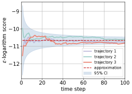
(a) $\epsilon$=0.01

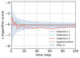
(b) $\epsilon$=0.1

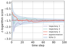
(c) $\epsilon$=1

Figure 1: $\epsilon$-logarithm score $\bar{\mathcal{L}}_{\epsilon}(p_{\mathbf{x}_{1:T},x_{1:T}})$ v.s. the time step $T$: for each $\epsilon$, three individual trajectories are randomly chosen for presentation; the blue transparent areas represent the $95$ confidence intervals, which are evaluated based on the sample variance of the scores on $100,000$ trajectories; the red-dotted line is pre-calculated based on Theorem 4 before simulations.

7 Simulation

In this section, we evaluate the $\epsilon$-logarithm score on a randomly generated linear SDS driven by Gaussian noises. The goals of our simulations are two-fold: first, under the assumption that the predictor is optimal, we verify the fact that the optimal expected $\epsilon$-logarithm score can be approximated by $d_{x}\log(2\epsilon)-\mathrm{H}_{\mathrm{d}}(p_{\mathbf{w}})$ with an error of scale $\mathcal{O}(\epsilon)$. Second, we verify the converging speed of $\bar{\mathcal{L}}(p_{\mathbf{x}_{1:T}},x_{1:T})$ on any given individual trajectory $x_{1:T}$ is of scale $\mathcal{O}(T^{-\frac{1}{2}})$ in the sense of probability.

7.1 Simulation Setup

We consider a two-dimensional linear SDS as follows.

$$\begin{array}[]{cc}\Phi:\begin{array}[]{lcl}x_{k+1}&=&Fx_{k}+w_{k},\quad w_{k}\overset{\text{i.i.d}}{\sim}\mathcal{N}(0,I).\end{array}\end{array}$$

The time step of each trajectory is $100$, and we randomly generate $100,000$ state trajectories of $\Phi$ starting from a random initial state. Choosing the neighborhood radius $\epsilon$ as $0.01,0.1,1$, we calculate the $\epsilon$-logarithm score $\bar{\mathcal{L}}_{\epsilon}$ for each state trajectory respectively.

7.2 Results and Analysis

First, the approximation accuracy of the optimal $\epsilon$-logarithm is verified to be of scale $\mathcal{O}(\epsilon)$. As Fig. 1 shows, the scores of three randomly generated individual trajectories converge to the same red dotted line (which is calculated before simulation, thus independent of the score on any trajectory). Moreover, according to the $95$ confidence intervals, the approximation error for each $\epsilon$ is of the same scale as $\epsilon$. Therefore, Theorem 4 indeed gives an effective approximation to the optimal $\epsilon$-logarithm score, and the approximation error suffices to characterize the system’s probabilistic predictability.

Second, Fig. 1 shows that all individual trajectories approach fast to the red dotted lines in less than $20$ time steps. This quick convergence is ensured by Theorem 5 in the sense of probability. The fact that different trajectories generated from the same SDS hold the same asymptotic decaying rate has reconfirmed the advantages of the $\epsilon$-logarithm score. Theoretically, Since this score is defined directly from probabilistic prediction performance and does not depend on specific state trajectory generated from an SDS, it views different trajectories as having the same predictability. Practically, benefiting from the quick convergence property of the score on individual trajectories, evaluating the expected score is easy to implement on one trajectory without the need for repeated samplings of different trajectories.

8 Conclusion

In this paper, we have proposed an $\epsilon$-logarithm score as a means to assess the quality of probabilistic predictions in stochastic dynamical systems (SDSs). By considering a neighborhood with radius $\epsilon$, our score generalizes the logarithm score and provides a comprehensive evaluation metric. Through formal evaluation and a discrete approximation method, we have demonstrated that the $\epsilon$-logarithm score is proper. We have further characterized the probabilistic predictability of an SDS by deriving the optimal expected score and providing an approximation with an error of scale $\mathcal{O}(\epsilon)$. This approximation has allowed us to quantitatively analyze how the predictability of the system depends on the neighborhood radius, differential entropies of process noises, and system dimension. Additionally, we have investigated the asymptotic convergence behavior of our score on individual trajectories. Our analysis has shown that the score converges to the probabilistic predictability when the process noises are independent and identically distributed, with a convergence speed of scale $\mathcal{O}(T^{-\frac{1}{2}})$ with respect to the trajectory length $T$. Finally, we have demonstrated the practical implications of our predictability analysis by designing unpredictable SDSs. Overall, our findings contribute to a deeper understanding of probabilistic prediction evaluation and offer valuable insights for the design and assessment of stochastic dynamical systems.

Appendix A Proof of Lemma 1

According to the definition of $\mathcal{L}_{\Sigma}$, one has

$$\mathcal{L}_{\Sigma}(\hat{p}_{\mathbf{x}},p_{\mathbf{x}}) =\mathbb{E}_{x}\log\hat{p}_{\mathbf{x}}^{\Sigma}(\Theta_{\Sigma}(x))$$

$$\overset{(i)}{=}\int_{\mathcal{X}}p_{\mathbf{x}}(x)\log\hat{p}_{\mathbf{x}}^{\Sigma}(\Theta_{\Sigma}(x))\mathrm{d}x$$

$$\overset{(ii)}{=}\sum_{i=1}^{N}\int_{A_{i}}p_{\mathbf{x}}(x)\log\hat{p}_{\mathbf{x}}^{\Sigma}(\Theta_{\Sigma}(x))\mathrm{d}x$$

$$\overset{(iii)}{=}\sum_{i=1}^{N}p_{\mathbf{x}}^{\Sigma}(i)\log\hat{p}_{\mathbf{x}}^{\Sigma}(i)$$

$$=\sum_{i=1}^{N}p_{\mathbf{x}}^{\Sigma}(i)\log\frac{\hat{p}_{\mathbf{x}}^{\Sigma}(i)}{p_{\mathbf{x}}^{\Sigma}(i)}+p_{\mathbf{x}}^{\Sigma}(i)\log p_{\mathbf{x}}^{\Sigma}(i)$$

$$\overset{(iv)}{=}-\mathrm{H}_{\mathrm{s}}(p_{\mathbf{x}}^{\Sigma})-D_{\mathcal{KL}}(p_{\mathbf{x}}^{\Sigma}||\hat{p}_{\mathbf{x}}^{\Sigma}),$$

where equality $(i)$ follows from the definition; $(ii)$ holds by first decomposing the set $\mathcal{X}$ based on the partition $\Sigma$ and then doing integration parts by parts; $(iii)$ holds according to the property of the label function that $\Theta_{\Sigma}(x)=i\;\forall x\in A_{i}$; (iv) follows from the definitions of Shannon entropy and discrete KL-divergence.

Appendix B Proof of Lemma 1

To begin with, we view the probabilistic prediction measured by $\mathcal{L}_{\epsilon}(\hat{p}_{\mathbf{x}},p_{\mathbf{x}})$ from a sequential sampling perspective between the predictor and the system. At each round $r\in\{1,\ldots,R\}$, the system randomly samples $x^{r}$ from the distribution $p_{\mathbf{x}}$, a score $\mathcal{L}_{\epsilon}^{(r)}(\hat{p}_{\mathbf{x}},p_{\mathbf{x}})$ is initialized by

$$\left\{\begin{array}[]{lr}\mathcal{L}_{\epsilon}^{(r)}(\hat{p}_{\mathbf{x}},p_{\mathbf{x}})\leftarrow\frac{r-1}{r}\mathcal{L}_{\epsilon}^{(r-1)}(\hat{p}_{\mathbf{x}},p_{\mathbf{x}})&r\geq 1,\\ \mathcal{L}_{\epsilon}^{(0)}(\hat{p}_{\mathbf{x}},p_{\mathbf{x}})\leftarrow 0&r=0.\end{array}\right.$$

Then the predictor samples $\hat{x}_{k}^{r}\overset{i.i.d}{\sim}\hat{p}_{\mathbf{x}}$ starting from $k=1$ to $K$. At each step $k$, a temporary score $\mathcal{L}_{\epsilon}^{(r,k)}(\hat{p}_{\mathbf{x}},p_{\mathbf{x}})$ is initialized by

$$\left\{\begin{array}[]{lr}\mathcal{L}_{\epsilon}^{(r,k)}(\hat{p}_{\mathbf{x}},p_{\mathbf{x}})\leftarrow\frac{k-1}{k}\mathcal{L}_{\epsilon}^{(r,k-1)}(\hat{p}_{\mathbf{x}},p_{\mathbf{x}})&k\geq 1,\\ \mathcal{L}_{\epsilon}^{(r,0)}(\hat{p}_{\mathbf{x}},p_{\mathbf{x}})\leftarrow 0&k=0.\end{array}\right.$$

If there is $\|\hat{x}_{k}^{r}-x^{r}\|\leq\epsilon$, the gain $\mathcal{K}_{k}^{r}=1$, else $\mathcal{K}_{k}^{r}=0$. Next, the score is updated by

$$\mathcal{L}_{\epsilon}^{(r,k)}(\hat{p}_{\mathbf{x}},p_{\mathbf{x}})\leftarrow\mathcal{L}_{\epsilon}^{(r,k)}(\hat{p}_{\mathbf{x}},p_{\mathbf{x}})+\frac{1}{k}\mathcal{K}_{k}^{r}.$$

The final update at the end of round $r$ is:

$$\mathcal{L}_{\epsilon}^{(r)}(\hat{p}_{\mathbf{x}},p_{\mathbf{x}})\leftarrow\mathcal{L}_{\epsilon}^{(r)}(\hat{p}_{\mathbf{x}},p_{\mathbf{x}})+\frac{1}{r}\mathcal{L}_{\epsilon}^{(r,K)}(\hat{p}_{\mathbf{x}},p_{\mathbf{x}}).$$

As both $R$ and $K$ asymptotically approach infinity, there is

$$\lim\limits_{R,K\to\infty}\mathcal{L}_{\epsilon}^{(R,K)}(\hat{p}_{\mathbf{x}},p_{\mathbf{x}})$$

$$\overset{(i)}{=} \lim\limits_{R\to\infty}\frac{1}{R}\sum_{r=1}^{R}\log\left(\lim\limits_{K\to\infty}\frac{1}{K}\sum_{k=1}^{K}\mathcal{K}_{k}^{r}\right)$$

$$\overset{(ii)}{\rightarrow} \lim\limits_{R\to\infty}\frac{1}{R}\sum_{r=1}^{R}\log\int_{\|\hat{x}-x^{r}\|\leq\epsilon}\hat{p}_{\mathbf{x}}(\hat{x})\mathrm{d}\hat{x}\text{ (a.s.)}$$

$$\overset{(iii)}{\rightarrow} \int_{\mathcal{X}}p_{\mathbf{x}}(x)\log\int_{\|\hat{x}-x\|\leq\epsilon}\hat{p}_{\mathbf{x}}(\hat{x})\mathrm{d}\hat{x}\mathrm{d}x\text{ (a.s.)}$$

$$\overset{(iv)}{=} \mathcal{L}_{\epsilon}(\hat{p}_{\mathbf{x}},p_{\mathbf{x}}),$$

where equation $(i)$ follows immediately from the above definitions on the sequential procedures; the convergences of $(ii)$ and $(iii)$ are ensured by the strong law of large numbers; equation (iv) follows from the definition of the expected $\epsilon$-logarithm score.

Similarly, we can also take a sequential sampling perspective on the probabilistic prediction measured by $\mathcal{L}_{\Sigma}(\hat{p}_{\mathbf{x}},p_{\mathbf{x}})$. At each round $r\in\{1,\ldots,R\}$, the system randomly samples $x^{r}$ from the distribution $p_{\mathbf{x}}$, a score $\mathcal{L}_{\Sigma}^{(r)}(\hat{p}_{\mathbf{x}},p_{\mathbf{x}})$ is initialized by

$$\left\{\begin{array}[]{lr}\mathcal{L}_{\Sigma}^{(r)}(\hat{p}_{\mathbf{x}},p_{\mathbf{x}})\leftarrow\frac{r-1}{r}\mathcal{L}_{\Sigma}^{(r-1)}(\hat{p}_{\mathbf{x}},p_{\mathbf{x}})&r\geq 1,\\ \mathcal{L}_{\Sigma}^{(0)}(\hat{p}_{\mathbf{x}},p_{\mathbf{x}})\leftarrow 0&r=0.\end{array}\right.$$

Then the predictor samples $\hat{x}_{k}^{r}\overset{i.i.d}{\sim}\hat{p}_{\mathbf{x}}$ starting from $k=1$ to $K$. At each step $k$, a temporary score $\mathcal{L}_{\Sigma}^{(r,k)}(\hat{p}_{\mathbf{x}},p_{\mathbf{x}})$ is initialized by

$$\left\{\begin{array}[]{lr}\mathcal{L}_{\Sigma}^{(r,k)}(\hat{p}_{\mathbf{x}},p_{\mathbf{x}})\leftarrow\frac{k-1}{k}\mathcal{L}_{\Sigma}^{(r,k-1)}(\hat{p}_{\mathbf{x}},p_{\mathbf{x}})&k\geq 1,\\ \mathcal{L}_{\Sigma}^{(r,0)}(\hat{p}_{\mathbf{x}},p_{\mathbf{x}})\leftarrow 0&k=0.\end{array}\right.$$

If there is $\Theta_{\Sigma}(\hat{x}_{k}^{r})=\Theta_{\Sigma}(x^{r})$, the gain $\mathcal{K}_{k}^{r}=1$, else $\mathcal{K}_{k}^{r}=0$. Next, the score is updated by

$$\mathcal{L}_{\Sigma}^{(r,k)}(\hat{p}_{\mathbf{x}},p_{\mathbf{x}})\leftarrow\mathcal{L}_{\Sigma}^{(r,k)}(\hat{p}_{\mathbf{x}},p_{\mathbf{x}})+\frac{1}{k}\mathcal{K}_{k}^{r}.$$

The final update at the end of round $r$ is:

$$\mathcal{L}_{\Sigma}^{(r)}(\hat{p}_{\mathbf{x}},p_{\mathbf{x}})\leftarrow\mathcal{L}_{\Sigma}^{(r)}(\hat{p}_{\mathbf{x}},p_{\mathbf{x}})+\frac{1}{r}\mathcal{L}_{\Sigma}^{(r,K)}(\hat{p}_{\mathbf{x}},p_{\mathbf{x}}).$$

As both $R$ and $K$ asymptotically approach infinity, there is

$$\lim\limits_{R,K\to\infty}\mathcal{L}_{\Sigma}^{(R,K)}(\hat{p}_{\mathbf{x}},p_{\mathbf{x}})$$

$$\overset{(i)}{=} \lim\limits_{R\to\infty}\frac{1}{R}\sum_{r=1}^{R}\log\left(\lim\limits_{K\to\infty}\frac{1}{K}\sum_{k=1}^{K}\mathcal{K}_{k}^{r}\right)$$

$$\overset{(ii)}{=} \lim\limits_{R\to\infty}\frac{1}{R}\sum_{r=1}^{R}\log\hat{p}_{\mathbf{x}}^{\Sigma}(\Theta_{\Sigma}(x^{r}))\text{ (a.s.)}$$

$$\overset{(iii)}{=} \sum_{i=1}^{N}p_{\mathbf{x}}^{\Sigma}(i)\log\hat{p}_{\mathbf{x}}^{\Sigma}(i)\text{ (a.s.)}$$

$$\overset{(iv)}{=} \mathcal{L}_{\Sigma}(\hat{p}_{\mathbf{x}},p_{\mathbf{x}}),$$

where equation $(i)$ follows immediately from the above definitions on the sequential procedures; the convergences of $(ii)$ and $(iii)$ are ensured by the strong law of large numbers; equation (iv) follows from the definition of the expected $\Sigma$-logarithm score.

Then, we prove the left inequality. Given a partition $\Sigma$ with $\operatorname{diam}(\Sigma)\leq\epsilon$, $\Theta_{\Sigma}(\hat{x}_{k}^{r})=\Theta_{\Sigma}(x^{r})$ indicates the existence of a set $A\in\Sigma$ such that $\hat{x}_{k}^{r},x^{r}\in A$. It follows that $\|\hat{x}_{k}^{r}-x^{r}\|_{\infty}\leq\epsilon$ because $\operatorname{diam}(A)\leq\epsilon$. Therefore, once the diameter of $\Sigma$ is less than $\epsilon$, those samples with nonzero gain during the $\Sigma$-sequential prediction must also have non-zero gains during the $\epsilon$-sequential prediction. As a result, we have $\mathcal{L}_{\Sigma}(\hat{p}_{\mathbf{x}},p_{\mathbf{x}})\leq\mathcal{L}_{\epsilon}(\hat{p}_{\mathbf{x}},p_{\mathbf{x}})$ under the assumption that $\operatorname{diam}(\Sigma)\leq\epsilon$. Moreover, since $\Sigma$ can be any partition as long as $\operatorname{diam}(\Sigma)\leq\epsilon$, there is

$$\max\limits_{\{\Sigma|\operatorname{diam}(\Sigma)\leq\epsilon\}}\mathcal{L}_{\Sigma}^{(R,K)}(\hat{p}_{\mathbf{x}},p_{\mathbf{x}})\leq\mathcal{L}_{\epsilon}^{(R,K)}(\hat{p}_{\mathbf{x}},p_{\mathbf{x}})$$

$$\overset{R,K\to\infty}{\Longrightarrow}\max\limits_{\{\Sigma|\operatorname{diam}(\Sigma)\leq\epsilon\}}\mathcal{L}_{\Sigma}(\hat{p}_{\mathbf{x}},p_{\mathbf{x}})\leq\mathcal{L}_{\epsilon}(\hat{p}_{\mathbf{x}},p_{\mathbf{x}}).$$

Finally, when it comes to the extreme case where $\Sigma=\{\mathcal{X}\}$, trivially there is $\mathcal{L}_{\Sigma}(\hat{p}_{\mathbf{x}},p_{\mathbf{x}})=0.$ As a result,

$$\mathcal{L}_{\epsilon}(\hat{p}_{\mathbf{x}},p_{\mathbf{x}})\leq\max\limits_{\Sigma}\mathcal{L}_{\Sigma}(\hat{p}_{\mathbf{x}},p_{\mathbf{x}}),$$

and the proof is completed.

Appendix C Proof of Theorem 2

To begin with, we define some necessary preliminary settings. Let $\mathcal{S}$ be the space composed of all partitions of $\mathbb{R}^{d}$. To make $\mathcal{S}$ a metric space, we implement $\mathcal{S}$ with a partition distance metric $D(\cdot,\cdot)$ which is well studied in [35, 36]:

$$D(P,Q)=\min\left\{\mu(A^{c}):\emptyset\subset A\subseteq\mathbb{R}^{d},P^{A}=Q^{A}\right\},$$

where $P^{A}$ is a partition of set $A$ induced by $P$, i.e., if $P=\bigcup_{i=1}^{m}\{B_{i}\}$ then $P^{A}=\bigcup_{i=1}^{m}\{B_{i}\bigcap A\}$. Intuitively, partition distance $D(P,Q)$ is the minimum measure of set that must be deleted from $\mathbb{R}^{d}$, so that the two induced partitions ($P$ and $Q$ restricted to the remaining elements) are identical to each other. It’s trivial to verify that $D(\cdot,\cdot)$ satisfies all three requirement of a distance metric.

Consider a functional operator $\mathcal{F}:\mathcal{S}\to\mathbb{R}$ such that $\mathcal{F}(\Sigma)=\mathcal{L}_{\Sigma}(\hat{p}_{\mathbf{x}},p_{\mathbf{x}})$. According to Theorem 1, there is

$$\mathcal{F}(\Sigma)=-\mathrm{H}_{\mathrm{s}}(p_{\mathbf{x}}^{\Sigma})-D_{\mathcal{KL}}\left(p_{\mathbf{x}}^{\Sigma}||\hat{p}_{\mathbf{x}}^{\Sigma}\right).$$

Then, we prove that $\mathcal{F}$ is continuous in metric space $\mathcal{S}$ with the distance metric $D(\cdot,\cdot)$. Continuity means that, for any $\Sigma=\{A_{i}\}_{i=1}^{|\Sigma|}$ and any converging partition sequence $\left\{\Sigma^{n}=\{A_{i}^{n}\}_{i=1}^{|\Sigma^{n}|}\right\}$ where $\lim\limits_{n\to\infty}D(\Sigma^{n},\Sigma)=0$, there is $\lim\limits_{n\to\infty}\mathcal{F}(\Sigma^{n})=\mathcal{F}(\Sigma)$. According to the definition of the partition sequence convergence, given any $\gamma>0$, there exists $N\in\mathbb{N}$ such that for any $n>N$ we have $D(\Sigma^{n},\Sigma)<\gamma$. When $n>N$, we have $A_{t}^{n}\in\Sigma^{n}$ such that $\mu(A_{t}\Delta A_{t}^{n})\leq\gamma$ for any $t=1,\ldots,|\Sigma|$, where $\mu(\cdot)$ denotes the Lebesgue measure, and $\Delta$ denotes the symmetric difference between two sets. Notice that for all $i\in\mathbb{N}$, there is

$$\left|p_{\mathbf{x}}^{\Sigma}(i)-p_{\mathbf{x}}^{\Sigma^{n}}(i)\right|= \left|\int\nolimits_{A_{i}}p_{\mathbf{x}}(x)\mathrm{d}x-\int\nolimits_{A_{i}^{n}}p_{\mathbf{x}}(x)\mathrm{d}x\right|$$

$$\leq \int\nolimits_{A_{i}\Delta A_{i}^{n}}p_{\mathbf{x}}(x)\mathrm{d}x.$$

Notice that $\lim\limits_{n\to\infty}\mu(A_{i}\Delta A_{i}^{n})=0$, we have $\lim\limits_{n\to\infty}|p_{\mathbf{x}}^{\Sigma}(i)-p_{\mathbf{x}}^{\Sigma^{n}}(i)|=0.$ Similarly, there is $\lim\limits_{n\to\infty}|\hat{p}_{\mathbf{x}}^{\Sigma}(i)-\hat{p}_{\mathbf{x}}^{\Sigma^{n}}(i)|=0.$ Now that $H_{\mathrm{s}}(\cdot)$, $D_{\mathcal{KL}}(\cdot)$ are all continuous functionals, the continuity of $\mathcal{F}$ is immediately derived.

Finally, the bounded inequality (13) suggests the existence of $\Sigma_{a},\Sigma_{b}\in\mathcal{S}$ such that

$$\mathcal{L}_{\Sigma_{a}}(\hat{p}_{\mathbf{x}},p_{\mathbf{x}})\leq\mathcal{L}_{\epsilon}(\hat{p}_{\mathbf{x}},p_{\mathbf{x}})\leq\mathcal{L}_{\Sigma_{b}}(\hat{p}_{\mathbf{x}},p_{\mathbf{x}}).$$

Therefore, the intermediate value theorem [37] admits the existence of $\Sigma^{\star}\in\mathcal{S}$ such that

$$\mathcal{L}_{\epsilon}(\hat{p}_{\mathbf{x}},p_{\mathbf{x}})=\mathcal{L}_{\Sigma^{\star}}(\hat{p}_{\mathbf{x}},p_{\mathbf{x}}).$$

Appendix D Proof of Theorem 3

When $\epsilon=0$, the result trivially follows from the definition of the expected logarithm score. When $\epsilon>0$, an approximation to $\mathcal{L}_{\epsilon}(p_{\mathbf{x}},p_{\mathbf{x}})$ is needed. To begin with, we need some preliminary tools. First, we define an error functional $\delta_{\epsilon}:\mathcal{P}\to\mathbb{R}$ by

$$\delta_{\epsilon}(h):=\max\limits_{\|x_{1}-x_{2}\|_{\infty}\leq\epsilon}|\log(h(x_{1}))-\log(h(x_{2}))|,$$

where $x_{1},x_{2}\in\mathbb{R}^{d_{x}}$ are two arbitrary states and $h\in\mathcal{P}$ is a continuous PDF. Second, we define another functional operator $\rho:\mathcal{P}\to\mathbb{R}$ as the maximum value of the solution set of an inequality, i.e.,

$$\rho(h)=\max_{z\in\mathbb{R}}\left\{z:\left|d_{x}\log(\frac{2}{z})\right|\leq\delta_{z\epsilon}(h)\right\}.$$

Note that the above inequality holds when $z=2$, thus the solution set is not empty. Besides, when $h$ is bounded, $\delta_{z\epsilon}(h)$ is bounded and monotonically increasing with $z$, thus the solution set is upper bounded. Therefore, $\rho(h)$ is finite and only depends on $h$. Third, we denote the $\epsilon$ neighborhood of $x$ as set $\mathcal{N}_{\epsilon}(x):=\{y\mid\|y-x\|_{\infty}\leq\epsilon\}$. Now, we are prepared to approximate $\mathcal{L}_{\epsilon}(p_{\mathbf{x}},p_{\mathbf{x}})$.

Let $\Sigma^{\star}=\{A_{i}\}_{i=1}^{|\Sigma^{\star}|}$. According to the intermediate value theorem, for any $i=1,\ldots,|\Sigma^{\star}|$ there exists $a_{i}\in A_{i}$ such that $p_{\mathbf{x}}(a_{i})|A_{i}|=p_{\mathbf{x}}^{\Sigma^{\star}}(i)$, where $|A_{i}|$ denotes the Lebesgue volume of $A_{i}$. Without loss of generality, we let all $A_{i}$ be a cube with a diameter equaling $\kappa\epsilon$. It follows that

$$\mathcal{L}_{\epsilon}(p_{\mathbf{x}},p_{\mathbf{x}})= -H_{\mathrm{s}}(p_{\mathbf{x}}^{\Sigma^{\star}})=\sum\limits_{i=1}^{\infty}p_{\mathbf{x}}^{\Sigma^{\star}}(i)\log\{p_{\mathbf{x}}^{\Sigma^{\star}}(i)\}$$

$$= \sum\limits_{i=1}^{\infty}p_{\mathbf{x}}(a_{i})|A_{i}|\log\{p_{\mathbf{x}}(a_{i})|A_{i}|\}$$

$$= \sum\limits_{i=1}^{\infty}p_{\mathbf{x}}(a_{i})|A_{i}|\log\{p_{\mathbf{x}}(a_{i})\}$$

$$+ \sum\limits_{i=1}^{\infty}p_{\mathbf{x}}(a_{i})|A_{i}|\log\{|A_{i}|\}.$$

The second term above can be further formulated as

$$\sum\limits_{i=1}^{\infty}p_{\mathbf{x}}(a_{i})|A_{i}|\log\{|A_{i}|\}= d_{x}\log(\kappa\epsilon)\sum\limits_{i=1}^{\infty}p_{\mathbf{x}}(a_{i})|A_{i}|$$ (23)

$$= d_{x}\log(\kappa\epsilon)$$

The first term is a Darboux sum for the Riemann integration of the negative differential entropy of $p_{\mathbf{x}}$. Their difference can be formulated as

$$\left|\sum\limits_{i=1}^{\infty}p_{\mathbf{x}}(a_{i})|A_{i}|\log\{p_{\mathbf{x}}(a_{i})\}+\mathrm{H}_{\mathrm{d}}(p_{\mathbf{x}})\right|$$ (24)

$$= \left|\sum\limits_{i=1}^{\infty}|p_{\mathbf{x}}(a_{i})|A_{i}|\log\{p_{\mathbf{x}}(a_{i})\}-\int\nolimits_{A_{i}}p_{\mathbf{x}}(x)\log(p_{\mathbf{x}}(x))\mathrm{d}x\right|$$

$$= \left|\sum\limits_{i=1}^{\infty}\int\nolimits_{A_{i}}p_{\mathbf{x}}(x)\log\left(\frac{p_{\mathbf{x}}(x)}{p_{\mathbf{x}}(a_{i})}\right)\mathrm{d}x\right|.$$

For any positive $\tau\leq\frac{\epsilon}{2}$, $\exists M(\tau)>0$ s.t.

$$\left|\mathrm{H}_{\mathrm{d}}(p_{\mathbf{x}})+\int_{\mathcal{N}_{M(\tau)}(0)}p_{\mathbf{x}}(x)\log p_{\mathbf{x}}(x)\mathrm{d}x\right|\leq\tau.$$

Then, we decompose $p_{\mathbf{x}}$ into two parts such that $p_{\mathbf{x}}=q_{1}+q_{2}$, where $q_{1}=p_{\mathbf{x}}\circ\mathbb{I}_{\mathcal{N}_{M(\tau)}(0)}$. Applying this decomposition to the equation (24), we have

$$\left|\sum\limits_{i=1}^{\infty}p_{\mathbf{x}}(a_{i})|A_{i}|\log\{p_{\mathbf{x}}(a_{i})\}+\mathrm{H}_{\mathrm{d}}(p_{\mathbf{x}})\right|$$ (25)

$$\leq \left|\sum\limits_{i=1}^{\infty}\int\nolimits_{A_{i}}q_{1}(x)\log\left(\frac{q_{1}(x)}{q_{1}(a_{i})}\right)\mathrm{d}x\right|$$

$$+\left|\sum\limits_{i=1}^{\infty}\int\nolimits_{A_{i}}q_{2}(x)\log\left(\frac{q_{2}(x)}{q_{2}(a_{i})}\right)\mathrm{d}x\right|$$

$$\leq \sum\limits_{i=1}^{\infty}\left|\int\nolimits_{A_{i}}q_{1}(x)\mathrm{d}x\right|\delta_{\kappa\epsilon}(q_{1})+2\tau$$

$$\leq \delta_{\kappa\epsilon}(q_{1})+\epsilon$$

Combining equation (23) and equation (25), we have

$$|\mathcal{L}_{\epsilon}(p_{\mathbf{x}},p_{\mathbf{x}})+\mathrm{H}_{\mathrm{d}}(p_{\mathbf{x}})-d_{x}\log(\kappa\epsilon)|\leq\delta_{\kappa\epsilon}(q_{1})+\epsilon.$$ (26)

Equation (26) is quite close to our objection except for the $d\log(\kappa\epsilon)$ term. In fact,

$$|\mathcal{L}_{\epsilon}(p_{\mathbf{x}},p_{\mathbf{x}})+\mathrm{H}_{\mathrm{d}}(p_{\mathbf{x}})-d_{x}\log(2\epsilon)|$$ (27)

$$= \left|\mathcal{L}_{\epsilon}(p_{\mathbf{x}},p_{\mathbf{x}})+\mathrm{H}_{\mathrm{d}}(p_{\mathbf{x}})-d_{x}\log(\kappa\epsilon)-d_{x}\log(\frac{2}{\kappa})\right|$$

$$\leq \left|\mathcal{L}_{\epsilon}(p_{\mathbf{x}},p_{\mathbf{x}})+\mathrm{H}_{\mathrm{d}}(p_{\mathbf{x}})-d_{x}\log(\kappa\epsilon)\right|+\left|d_{x}\log(\frac{2}{\kappa})\right|$$

Hence, our final goal is to figure out an upper bound for $\left|d_{x}\log(\frac{2}{\kappa})\right|$. Following the sequential procedure notations in Lemma B, on the one hand, we have

$$\mathcal{L}_{\epsilon}^{(R,\infty)}(p_{\mathbf{x}},p_{\mathbf{x}})= \frac{1}{R}\sum_{r=1}^{R}\log\int_{\|x-x^{r}\|\leq\epsilon}p_{\mathbf{x}}(x)\mathrm{d}x$$

$$= \frac{1}{R}\sum_{r=1}^{R}\log\left\{(2\epsilon)^{d_{x}}(\bar{x}^{r})\right\},$$

where $\bar{x}^{r}\in\mathcal{N}_{\epsilon}(x^{r})$ satisfying

$$p_{\mathbf{x}}(\bar{x}^{r})=\frac{1}{(2\epsilon)^{d_{x}}}\int\nolimits_{\mathcal{N}_{\epsilon}(x^{r})}p_{\mathbf{x}}(x)\mathrm{d}x.$$

On the other hand,

$$\mathcal{L}_{\Sigma^{\star}}^{(R,\infty)}(p_{\mathbf{x}},p_{\mathbf{x}})= \frac{1}{R}\sum_{r=1}^{R}\log p_{\mathbf{x}}^{\Sigma}(\Theta_{\Sigma}(x^{r}))$$

$$= \frac{1}{R}\sum_{r=1}^{R}\log\left\{(\kappa\epsilon)^{d_{x}}p_{\mathbf{x}}(s_{\Theta(x^{r})})\right\},$$

where $s_{\Theta(x^{r})}\in A_{\Theta(x^{r})}$ satisfying

$$p_{\mathbf{x}}(s_{\Theta(x^{r})})=\frac{1}{(\kappa\epsilon)^{d_{x}}}\int\nolimits_{A_{\Theta(w_{k})}}p_{\mathbf{x}}(x)\mathrm{d}x.$$

It follows that

$$0 =\lim\limits_{R\to\infty}\mathcal{L}_{\epsilon}^{(R,\infty)}(p_{\mathbf{x}},p_{\mathbf{x}})-\mathcal{L}_{\Sigma^{\star}}^{(R,\infty)}(p_{\mathbf{x}},p_{\mathbf{x}})$$

$$=d_{x}\log\left(\frac{2}{\kappa}\right)+\lim\limits_{R\to\infty}\frac{1}{R}\sum\limits_{r=1}^{R}\log p_{\mathbf{x}}(\bar{x}_{r})-\log p_{\mathbf{x}}(s_{\Theta(x^{r})}).$$

Therefore,

$$\left|d\log(\frac{2}{\kappa})\right|\leq \lim\limits_{R\to\infty}\!\frac{1}{R}\!\sum\limits_{r=1}^{R}\left|\log p_{\mathbf{x}}(\bar{x}_{r})-\log p_{\mathbf{x}}(s_{\Theta(x^{r})})\right|$$

$$= \lim\limits_{R\to\infty}\frac{1}{R}\!\sum\limits_{r=1}^{R}\left|\log q_{1}(\bar{x}^{r})\!-\!\log q_{1}(s_{\Theta(x^{r})})\right|$$

$$+\!\frac{1}{R}\!\sum\limits_{r=1}^{R}\left|\log q_{2}(\bar{x}^{r})\!-\!\log q_{2}(s_{\Theta(x^{r})})\right|$$

$$\leq \delta_{\kappa\epsilon}(q_{1})+\epsilon$$

Moreover, since $\rho(q_{1})$ is the maximum solution to equation $|d\log(\frac{2}{x})|\leq\delta_{x\epsilon}(q_{1})$ with respect to $x$, we have $\delta_{\kappa\epsilon}(q_{1})\leq\delta_{\rho(q_{1})\epsilon}(q_{1})$. Applying this fact to equation (27), we have

$$|\mathcal{L}_{\epsilon}(p_{\mathbf{x}},p_{\mathbf{x}})+\mathrm{H}_{\mathrm{d}}(q)-d\log(2\epsilon)|\leq 2\left(\delta_{\rho(q_{1})\epsilon}(q_{1})+\epsilon\right).$$

Note that $\delta_{\rho(q_{1})\epsilon}(q_{1})$ reflects to what extent $q_{1}$ can vibrate in a local region with diameter less than $\rho(q_{1})\epsilon$. Since the support of $q_{1}$ is bounded, the probability distribution must be uniformly continuous, thus $\delta_{\rho(q_{1})\epsilon}(q_{1})=O(\epsilon)$. Then we have

$$|\mathcal{L}_{\epsilon}(p_{\mathbf{x}},p_{\mathbf{x}})+\mathrm{H}_{\mathrm{d}}(p_{\mathbf{x}})-d_{x}\log(2\epsilon)|=O(\epsilon).$$

The proof is completed.

Appendix E Proof of Theorem 4

When $\epsilon=0$, the result trivially follows from the definition of the expected logarithm score. When $\epsilon>0$, an approximation to $\mathcal{L}_{\epsilon}(p_{\mathbf{x}},p_{\mathbf{x}})$ is needed. Let $q_{x_{1:k-1}}(\cdot)=p_{\mathbf{x}_{k}\mid\mathbf{x}_{1:k-1}}(\cdot\mid x_{1:k-1})$, it follows that

$$\left|\bar{\mathcal{L}}_{\epsilon}(p_{\mathbf{x}_{1:T}},p_{\mathbf{x}_{1:T}})-\left\{d\log(2\epsilon)-\frac{1}{T}\mathrm{H}_{\mathrm{d}}(\mathbf{x}_{1:T})\right\}\right|$$

$$\overset{(i)}{=} \bigg{|}\frac{1}{T}\!\sum_{k=1}^{T}\mathbb{E}_{x_{1:k-1}}\mathcal{L}_{\epsilon}\left(q_{x_{1:k-1}},q_{x_{1:k-1}}\right)$$

$$-\left\{d\log(2\epsilon)-\frac{1}{T}\sum_{k=1}^{T}\mathrm{H}_{\mathrm{d}}(\mathbf{x}\mid\mathbf{x}_{1:k-1})\right\}\bigg{|}$$

$$\overset{(ii)}{\leq} \frac{1}{T}\!\sum_{k=1}^{T}\mathbb{E}_{x_{1:k-1}}\bigg{|}\mathcal{L}_{\epsilon}\left(q_{x_{1:k-1}},q_{x_{1:k-1}}\right)-$$

$$\left\{d\log(2\epsilon)-\mathrm{H}_{\mathrm{d}}(\mathbf{x}\mid x_{1:k-1})\right\}\bigg{|}$$

$$\overset{(iii)}{=} \mathcal{O}(\epsilon),$$

where equation $(i)$ follows from the definition of $\bar{\mathcal{L}}_{\epsilon}$ and the property of conditional entropy, inequality $(ii)$ follows from the absolute value inequality and equation $(iii)$ holds because Lemma 3 ensures each term is $\mathcal{O}(\epsilon)$, thus the average of finite sum is also of the scale $\mathcal{O}(\epsilon)$.

Appendix F Proof of Theorem 5

Based on the assumption that the process noises are i.i.d and the definition of $\bar{\mathcal{L}}_{\epsilon}$, one has

$$\bar{\mathcal{L}}_{\epsilon}(p_{\mathbf{x}_{1:T}},x_{1:T})= \frac{1}{T}\!\sum_{k=1}^{T}\mathcal{L}_{\epsilon}\left(p_{\mathbf{x}_{k}\mid\mathbf{x}_{1:k-1}}(\cdot\mid x_{1:k-1}),x_{k}\right)$$

$$\overset{(i)}{=} \frac{1}{T}\!\sum_{k=1}^{T}\mathcal{L}_{\epsilon}\left(p_{\mathbf{x}_{k}\mid\mathbf{x}_{k-1}}(\cdot\mid x_{k-1}),x_{k}\right)$$

$$\overset{(ii)}{=} \frac{1}{T}\!\sum_{k=1}^{T}\mathcal{L}_{\epsilon}\left(p_{\mathbf{w}},w_{k}\right)$$

$$\overset{(iii)}{\rightarrow} \mathcal{L}_{\epsilon}\left(p_{\mathbf{w}},p_{\mathbf{w}}\right)\text{ (a.s.)},$$

where equation $(i)$ holds because when the process noises $\{\mathbf{w}_{k}\}_{k=1}^{T}$ are independent, $\{\mathbf{x}_{k}\}_{k=1}^{T}$ is a Markov process, thus $p_{\mathbf{x}_{k}\mid\mathbf{x}_{1:k-1}}=p_{\mathbf{x}_{k}\mid\mathbf{x}_{k-1}}$; equation $(ii)$ holds because the conditional distribution is determined by the distribution of $\mathbf{w}_{k}$, which is identically distributed to PDF $p_{\mathbf{w}}$. The convergence $(iii)$ is ensured by the strong law of large numbers. Moreover, if $\mathbb{E}_{w\sim p_{\mathbf{w}}}\mathcal{L}_{\epsilon}(p_{\mathbf{w}},w)^{2}<\infty$, it follows that

$$\operatorname{Var}\{\bar{\mathcal{L}}_{\epsilon}(p_{\mathbf{x}_{1:T}},x_{1:T})\}=\operatorname{Var}\left\{\frac{1}{T}\!\sum_{k=1}^{T}\mathcal{L}_{\epsilon}\left(p_{\mathbf{w}},w_{k}\right)\right\}$$

$$= \frac{1}{T}\left\{\mathbb{E}_{w\sim p_{\mathbf{w}}}\mathcal{L}_{\epsilon}(p_{\mathbf{w}},w)^{2}-\mathcal{L}_{\epsilon}(p_{\mathbf{w}},p_{\mathbf{w}})^{2}\right\}.$$

Ensured by the Chebyshev inequality, the converging speed is $\mathcal{O}_{p}(\frac{1}{\sqrt{T}})$, i.e., $\forall\delta>0$, there is

$$\operatorname{Pr}\left\{|\bar{\mathcal{L}}_{\epsilon}(p_{\mathbf{x}_{1:T}},x_{1:T})-\mathcal{L}_{\epsilon}(p_{\mathbf{w}},p_{\mathbf{w}})|\geq\delta\right\}=\mathcal{O}(\frac{1}{\sqrt{T}}).$$

Appendix G Proof of Theorem 6

Because $D$ is diagonal, we can focus on the distribution design for each dimension separately. First, we define the Lagrange function,

$$\mathcal{L}(q,\lambda_{0},\lambda_{1},\lambda_{2})$$

$$= \mathrm{H}_{\mathrm{d}}(q)+\lambda_{0}(\int_{-\infty}^{\infty}q(x)\mathrm{d}x-1)+\lambda_{1}(\int_{-\infty}^{\infty}xq(x)\mathrm{d}x-0)$$

$$+\lambda_{2}(\int_{-\infty}^{\infty}x^{2}q(x)\mathrm{d}x-\sigma^{2}).$$

By KKT conditions we get

$$\text{(KKT):}\left\{\begin{array}[]{cl}&\log(q)+1=\lambda_{0}+\lambda_{1}x+\lambda_{2}x^{2}\\ &\int_{-N}^{N}q(x)\mathrm{d}x=1\\ &\int_{-N}^{N}xq(x)\mathrm{d}x=0\\ &\int_{-N}^{N}x^{2}q(x)\mathrm{d}x=\sigma^{2}.\\ \end{array}\right.$$

The first KKT condition shows that

$$q(x)=te^{\lambda x^{2}}\mathbb{I}_{[-N,N]}(x).$$

Substituting this into other KKT conditions we have

$$\left\{\begin{aligned} &\int_{-N}^{N}te^{\lambda x^{2}}\mathrm{d}x=1\\ &\int_{-N}^{N}tx^{2}e^{\lambda x^{2}}\mathrm{d}x=\sigma^{2}.\end{aligned}\right.$$

Our goal is to solve these equations to get $\lambda,t$, the second equation can be transformed as follows

$$\int_{-N}^{N}tx^{2}e^{\lambda x^{2}}\mathrm{d}x= 2\left[\frac{tx}{2\lambda}e^{\lambda x^{2}}\bigg{|}_{0}^{N}-\int_{0}^{N}\frac{t}{2\lambda}e^{\lambda x^{2}}\mathrm{d}x\right]$$

$$= \frac{tN}{\lambda}e^{\lambda N^{2}}-\frac{1}{2\lambda}=\sigma^{2}$$

$$\Rightarrow t= \frac{1+2\sigma^{2}\lambda}{2Ne^{N^{2}\lambda}}.$$

Substituting this into the first equation, we can then focus on the solution of this integral equation:

$$\int_{-N}^{N}\frac{1+2\sigma^{2}\lambda}{2Ne^{N^{2}\lambda}}e^{\lambda x^{2}}\mathrm{d}x=1.$$

If $\lambda=0$, it’s easy to show that only uniform distribution is possible, and $N=\sqrt{3}\sigma$ is the solution. Therefore the distribution is

$$\frac{1}{2\sqrt{3}\sigma}\mathbb{I}_{[-\sqrt{3}\sigma,\sqrt{3}\sigma]}.$$

If $\lambda\neq 0$, suppose $N\geq\sqrt{3}\sigma$. On the one hand, we have

$$\frac{1+2\sigma^{2}\lambda}{2Ne^{N^{2}\lambda}}\leq\frac{1+2\sigma^{2}\lambda}{2\sqrt{3}\sigma e^{3\sigma^{2}\lambda}}\leq\frac{1+2\sigma^{2}\lambda}{2\sqrt{3}\sigma(1+3\sigma^{2}\lambda)}\leq \frac{1}{2\sqrt{3}\sigma},$$

which indicates that

$$q(x)\leq\frac{1}{2\sqrt{3}\sigma},~{}\forall x\in[-N,N].$$

On the other hand,

$$\int_{-N}^{N}x^{2}q(x)\mathrm{d}x=\sigma^{2}$$

$$\Rightarrow \int_{-N}^{N}x^{2}q(x)\mathrm{d}x=\int_{-\sqrt{3}\sigma}^{\sqrt{3}\sigma}x^{2}\frac{1}{2\sqrt{3}\sigma}\mathrm{d}x$$

$$\Rightarrow \int_{-\sqrt{3}\sigma}^{\sqrt{3}\sigma}x^{2}\left(\frac{1}{2\sqrt{3}\sigma}-q(x)\right)\mathrm{d}x=2\int_{\sqrt{3}\sigma}^{N}x^{2}q(x)\mathrm{d}x$$

$$\Rightarrow \frac{\int_{-\sqrt{3}\sigma}^{\sqrt{3}\sigma}x^{2}\left(\frac{1}{2\sqrt{3}\sigma}-q(x)\right)\mathrm{d}x}{\int_{-\sqrt{3}\sigma}^{\sqrt{3}\sigma}\frac{1}{2\sqrt{3}\sigma}-q(x)\mathrm{d}x}=\frac{\int_{\sqrt{3}\sigma}^{N}x^{2}q(x)\mathrm{d}x}{\int_{\sqrt{3}\sigma}^{N}q(x)\mathrm{d}x}.$$

However, the fact that $\text{l.h.s}\leq 3\sigma^{2}$ and $\text{r.h.s}>3\sigma^{2}$ leads to contradiction.

If $N<\sqrt{3}\sigma$, on the one hand it follows that

$$\int_{-N}^{N}q(x)dx=\int_{-\sqrt{3}\sigma}^{\sqrt{3}\sigma}q(x)\mathrm{d}x,$$

then there is $q(0)>\frac{1}{2\sqrt{3}\sigma}.$ Suppose $q(m)=\frac{1}{2\sqrt{3}\sigma}$, then $q(x)\geq\frac{1}{2\sqrt{3}\sigma}\;\forall x\in[-m,m],$ and $q(x)\leq\frac{1}{2\sqrt{3}\sigma}\;\forall x\notin[-m,m].$

On the other hand,

$$\int_{-N}^{N}\!x^{2}q(x)\mathrm{d}x\!=\!\sigma^{2}\Rightarrow\int_{-N}^{N}\!x^{2}q(x)\mathrm{d}x\!=\!\int_{-\sqrt{3}\sigma}^{\sqrt{3}\sigma}\!x^{2}\frac{1}{2\sqrt{3}\sigma}\mathrm{d}x$$

Therefore, we have

$$\int_{-m}^{m}\!\!x^{2}\left(q(x)\!-\!\frac{1}{2\sqrt{3}\sigma}\right)\!\mathrm{d}x\!=\!2\int_{m}^{\sqrt{3}\sigma}\!\!\!x^{2}\left(\frac{1}{2\sqrt{3}\sigma}\!-\!q(x)\right)\!\mathrm{d}x,$$

$$\frac{\int_{-m}^{m}x^{2}\left(q(x)-\frac{1}{2\sqrt{3}\sigma}\right)\mathrm{d}x}{\int_{-m}^{m}q(x)-\frac{1}{2\sqrt{3}\sigma}\mathrm{d}x}=\frac{\int_{m}^{\sqrt{3}\sigma}x^{2}\left(\frac{1}{2\sqrt{3}\sigma}-q(x)\right)\mathrm{d}x}{\int_{m}^{\sqrt{3}\sigma}\frac{1}{2\sqrt{3}\sigma}-q(x)\mathrm{d}x}.$$

Again, the fact that $\text{l.h.s}<m^{2}$ and $\text{r.h.s}\geq m^{2}$ leads to contradiction. Therefore, the solution to KKT conditions must be uniform distribution.

Appendix H Proof of Theorem 7

Optimization problem $\mathbb{P}_{2}$ can be reformed as

$$\max_{q}\min_{u}~{}g_{r}(q,u)\quad$$

s.t. $$\left\{\begin{aligned} &g_{r}(q,u)=-\log\int\nolimits_{B_{u}(r)}q(x)\mathrm{d}x,\\ &E(q)=0,\operatorname{Var}(q)=\sigma^{2},\mu(\operatorname{supp}(q))<\infty.\end{aligned}\right.$$

Notice that,

$$\min_{u}~{}g_{r}(q,u)$$

$$= \min_{h}\int_{-\infty}^{\infty}g_{r}(q,u)h(u)\mathrm{d}u$$

$$= \min_{h}\int_{-\infty}^{\infty}-\log\left[\int\nolimits_{B_{u}(r)}q(x)dx\right]h(u)\mathrm{d}u$$

$$= \min_{h}\int_{-\infty}^{\infty}-\log\left[\frac{\int\nolimits_{B_{u}(r)}q(x)dx}{q(u)\cdot 2r}\cdot q(u)\cdot 2r\right]h(u)\mathrm{d}u$$

$$= \min_{h}D_{\mathcal{KL}}(h||q)+\mathrm{H}_{\mathrm{d}}(h)-\log(2r)+K(q,h,r).$$

Now we can consider this functional optimization problem

$$\max_{q}\min_{h}~{}D_{\mathcal{KL}}(h||q)+\mathrm{H}_{\mathrm{d}}(h)+\log(2r)+K(q,h,r)$$

s.t. $$\left\{\begin{aligned} &K(q,h,r)=\int h(u)\log\left[\frac{\int\nolimits_{B_{u}(r)}q(x)dx}{q(u)\cdot 2r}\right]\mathrm{d}u,\\ &E(q)=0,\operatorname{Var}(q)=\sigma^{2},\mu(\operatorname{supp}(q))<\infty.\end{aligned}\right.$$

Construct a decreasing convergent sequence $\{r_{n}\}_{n=1}^{\infty}$ such that $\lim\limits_{n\rightarrow\infty}r_{n}=0$ and it is easy to show that $\lim\limits_{n\rightarrow\infty}K(f,h,r_{n})=0$. Therefore problem $\mathbb{P}_{2}$ is equivalent to the following problem

$$\max_{q}\min_{h}~{}D_{\mathcal{KL}}(h||q)+\mathrm{H}_{\mathrm{d}}(h)$$

s.t. $$E(q)=0,\operatorname{Var}(q)=\sigma^{2},\mu(\operatorname{supp}(q))<\infty.$$

Immediately, there is

$$\min_{h}D_{\mathcal{KL}}(h||q)+\mathrm{H}_{\mathrm{d}}(h)\leq D_{\mathcal{KL}}(q||q)+\mathrm{H}_{\mathrm{d}}(h)=\mathrm{H}_{\mathrm{d}}(q),$$

and the equality holds when $q$ is a uniform distribution. Moreover, Theorem 6 shows that the solution to problem $\mathbb{P}_{1}$ is uniform distribution, we have

$$\max_{q}\min_{h}~{}D_{\mathcal{KL}}(h||q)+\mathrm{H}_{\mathrm{d}}(h)$$

$$\leq \max_{q}\mathrm{H}_{\mathrm{d}}(q)$$

$$= \mathrm{H}_{\mathrm{d}}(q^{\star}),$$

where $q^{\star}=\frac{1}{2\sqrt{3}\sigma}\mathbb{I}_{[-\sqrt{3}\sigma,\sqrt{3}\sigma]}$. Therefore, these two optimization problems are equivalent in the one-dimension condition.

References

- [1] T. Xu and J. He, “Predictability of stochastic dynamical system: A probabilistic perspective,” in 2022 IEEE 61st Conference on Decision and Control (CDC), pp. 5466–5471, Dec. 2022.
- [2] D. Landgraf, A. Völz, F. Berkel, K. Schmidt, T. Specker, and K. Graichen, “Probabilistic prediction methods for nonlinear systems with application to stochastic model predictive control,” Annual Reviews in Control, vol. 56, p. 100905, Jan. 2023.
- [3] T. Gneiting and A. E. Raftery, “Strictly proper scoring rules, prediction, and estimation,” Journal of the American Statistical Association, vol. 102, pp. 359–378, Mar. 2007.
- [4] T. Gneiting and M. Katzfuss, “Probabilistic forecasting,” Annual Review of Statistics and Its Application, vol. 1, no. 1, pp. 125–151, 2014.
- [5] A. Carvalho, “An overview of applications of proper scoring rules,” Decision Analysis, vol. 13, pp. 223–242, Dec. 2016.
- [6] R. Buizza, “The value of probabilistic prediction,” Atmospheric Science Letters, vol. 9, no. 2, pp. 36–42, 2008.
- [7] P. Djuric, J. Kotecha, J. Zhang, Y. Huang, T. Ghirmai, M. Bugallo, and J. Miguez, “Particle filtering,” IEEE Signal Processing Magazine, vol. 20, pp. 19–38, Sept. 2003.
- [8] B. Kouvaritakis, M. Cannon, S. V. Raković, and Q. Cheng, “Explicit use of probabilistic distributions in linear predictive control,” Automatica, vol. 46, pp. 1719–1724, Oct. 2010.
- [9] T. Sauder, S. Marelli, and A. J. Sørensen, “Probabilistic robust design of control systems for high-fidelity cyber–physical testing,” Automatica, vol. 101, pp. 111–119, Mar. 2019.
- [10] C. E. Roelofse and C. E. van Daalen, “An accurate and efficient approach to probabilistic conflict prediction,” Automatica, vol. 153, p. 111021, July 2023.
- [11] J. Li, J. He, Y. Li, and X. Guan, “Unpredictable trajectory design for mobile agents,” in 2020 American Control Conference (ACC), pp. 1471–1476, July 2020.
- [12] E. N. Lorenz, “Predictability: A problem partly solved,” in Proc. Seminar on Predictability, vol. 1, 1996.
- [13] G. Boffetta, M. Cencini, M. Falcioni, and A. Vulpiani, “Predictability: A way to characterize complexity,” Physics Reports, vol. 356, pp. 367–474, Jan. 2002.
- [14] T. N. Palmer, “Predicting uncertainty in forecasts of weather and climate,” Reports on Progress in Physics, vol. 63, pp. 71–116, Jan. 2000.
- [15] E. Kalnay, Atmospheric Modeling, Data Assimilation and Predictability. Cambridge university press, 2003.
- [16] J. Slingo and T. Palmer, “Uncertainty in weather and climate prediction,” Philosophical Transactions of the Royal Society A: Mathematical, Physical and Engineering Sciences, vol. 369, pp. 4751–4767, Dec. 2011.
- [17] F. Biondi, A. Legay, B. F. Nielsen, and A. Wąsowski, “Maximizing entropy over markov processes,” Journal of Logical and Algebraic Methods in Programming, vol. 83, pp. 384–399, Sept. 2014.
- [18] T. Chen and T. Han, “On the complexity of computing maximum entropy for markovian models,” 34th International Conference on Foundation of Software Technology and Theoretical Computer Science (FSTTCS 2014), vol. 29, pp. 571–583, 2014.
- [19] Y. Savas, M. Ornik, M. Cubuktepe, M. O. Karabag, and U. Topcu, “Entropy maximization for markov decision processes under temporal logic constraints,” IEEE Transactions on Automatic Control, vol. 65, pp. 1552–1567, Apr. 2020.
- [20] Y. Savas, M. Hibbard, B. Wu, T. Tanaka, and U. Topcu, “Entropy maximization for partially observable markov decision processes,” IEEE Transactions on Automatic Control, pp. 1–8, 2022.
- [21] M. Hibbard, Y. Savas, B. Wu, T. Tanaka, and U. Topcu, “Unpredictable planning under partial observability,” in 2019 IEEE 58th Conference on Decision and Control (CDC), pp. 2271–2277, Dec. 2019.
- [22] C. Song, Z. Qu, N. Blumm, and A.-L. Barabási, “Limits of predictability in human mobility,” Science, vol. 327, no. 5968, pp. 1018–1021, 2010.
- [23] Y. Li, D. Jin, P. Hui, Z. Wang, and S. Chen, “Limits of predictability for large-scale urban vehicular mobility,” IEEE Transactions on Intelligent Transportation Systems, vol. 15, pp. 2671–2682, Dec. 2014.
- [24] C. Zhang, K. Zhao, and M. Chen, “Beyond the limits of predictability in human mobility prediction: Context-transition predictability,” IEEE Transactions on Knowledge and Data Engineering, pp. 1–1, 2022.
- [25] H. Wang, S. Zeng, Y. Li, and D. Jin, “Predictability and prediction of human mobility based on application-collected location data,” IEEE Transactions on Mobile Computing, vol. 20, pp. 2457–2472, July 2021.
- [26] T. DelSole, “Predictability and information theory. part i: Measures of predictability,” Journal of the Atmospheric Sciences, vol. 61, pp. 2425–2440, Oct. 2004.
- [27] T. DelSole, “Predictability and information theory. part ii: Imperfect forecasts,” Journal of the Atmospheric Sciences, vol. 62, pp. 3368–3381, Sept. 2005.
- [28] T. DelSole and M. K. Tippett, “Predictability: Recent insights from information theory,” Reviews of Geophysics, vol. 45, no. 4, 2007.
- [29] C. Byrnes, A. Lindquist, and T. McGregor, “Predictability and unpredictability in kalman filtering,” IEEE Transactions on Automatic Control, vol. 36, pp. 563–579, May 1991.
- [30] S. Yasini and K. Pelckmans, “Worst-case prediction performance analysis of the kalman filter,” IEEE Transactions on Automatic Control, vol. 63, pp. 1768–1775, June 2018.
- [31] J. M. Bernardo, “Expected information as expected utility,” The Annals of Statistics, vol. 7, no. 3, pp. 686–690, 1979.
- [32] A. P. Dawid, “The geometry of proper scoring rules,” Annals of the Institute of Statistical Mathematics, vol. 59, pp. 77–93, Feb. 2007.
- [33] M. Parry, A. P. Dawid, and S. Lauritzen, “Proper local scoring rules,” The Annals of Statistics, vol. 40, Feb. 2012.
- [34] MTCAJ. Thomas and A. T. Joy, Elements of Information Theory. Wiley-Interscience, 2006.
- [35] D. Gusfield, “Partition-distance: A problem and class of perfect graphs arising in clustering,” Information Processing Letters, vol. 82, pp. 159–164, May 2002.
- [36] G. Rossi, “Partition distances,” arXiv preprint arXiv:1106.4579, 2011.
- [37] W. Rudin, Principles of Mathematical Analysis, vol. 3. McGraw-hill New York, 1976.