Paths through Equally Spaced Points on a Circle

Abstract

Consider $n$ points evenly spaced on a circle, and a path of $n-1$ chords that uses each point once. There are $m=\lfloor n/2\rfloor$ possible chord lengths, so the path defines a multiset of $n-1$ elements drawn from $\{1,2,\ldots,m\}$. The first problem we consider is to characterize the multisets which are realized by some path. Buratti conjectured that all multisets can be realized when $n$ is prime, and a generalized conjecture for all $n$ was proposed by Horak and Rosa. Previously the conjecture was proved for $n\leq 19$ and $n=23$; we extend this to $n\leq 37$ (OEIS sequence A352568).

The second problem is to determine the number of distinct (euclidean) path lengths that can be realized. For this there is no conjecture; we extend current knowledge from $n\leq 16$ to $n\leq 37$ (OEIS sequence A030077). When $n$ is prime, twice a prime, or a power of 2, we prove that two paths have the same length only if they have the same multiset of chord lengths.

1 Introduction

Consider $n$ points equally spaced around a circle. There are $m=\lfloor n/2\rfloor$ possible chord lengths. The type of a chord is its position in the list of chord lengths in increasing order; thus a chord of type 1 is between two adjacent points and a chord of type $m$ is between two points as antipodal as possible. If the points are numbered cyclically, the type of the chord between points $i$ and $j$ is $\min\{\mathopen{|}i-j\mathclose{|},n-\mathopen{|}i-j\mathclose{|}\}$.

Now connect the points by a polygonal path using each point exactly once. The associated multiset of the path is the multiset of the types of the chords. We consider two questions:

(Q1) Which multisets are the associated multiset of some path?
(Q2) How many distinct (euclidean) lengths can paths have?

We denote a multiset by the notation $[\ell_{1},\ldots,\ell_{m}]$, where $\ell_{j}$ is the number of elements equal to $j$. Figure 1 shows the associated multiset of a path in this notation.

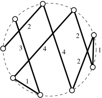
Figure 1: A path for $n=9$ with associated multiset $[2,3,1,2]$.

Three classes of multisets are relevant to this study.

• $\mathcal{M}_{n}$ is the class of all multisets $[\ell_{1},\ldots,\ell_{m}]$ such that $m=\lfloor n/2\rfloor$ and $\sum_{j=1}^{m}\ell_{j}=n-1$.

• The admissible multisets are the class $\mathcal{A}_{n}\subseteq\mathcal{M}_{n}$ of multisets with this additional property: for each divisor $d$ of $n$, $\sum_{j=1}^{\lfloor m/d\rfloor}\ell_{jd}\leq n-d$.

• The realizable multisets are the class $\mathcal{R}_{n}\subseteq\mathcal{M}_{n}$ of multisets associated with some path.

In 2007, Marco Buratti communicated to Alex Rosa the conjecture that $\mathcal{R}_{n}=\mathcal{M}_{n}$ if $n$ is prime [6]. Despite its simple statement, the conjecture remains open, though Mariusz Meszka confirmed it by computer for $n\leq 23$ [7]. It is easy to see that the primality of $n$ is essential for $\mathcal{R}_{n}=\mathcal{M}_{n}$, however Horak and Rosa proposed a more general conjecture that has drawn a lot of attention [6].

Conjecture 1 (Buratti–Horak–Rosa).

$\mathcal{R}_{n}=\mathcal{A}_{n}$ for $n\geq 1$.

Horak and Rosa noted that $\mathcal{R}_{n}\subseteq\mathcal{A}_{n}$; for a self-contained proof see Pasotti and Pellegrini [11]. Meszka confirmed the conjecture for $n\leq 18$ [7]. In addition, Conjecture 1 has been proved for a considerable number of special cases [2, 3, 9, 10, 11, 12, 14]. We will prove:

Theorem 2.

The Buratti–Horak–Rosa conjecture is true for $n\leq 37$.

For question Q2, the first investigation we are aware of was carried out in the mid-1980s by Daniel Gittelson, then at the University of Michigan School of Medicine. Gittelson found the counts up to 12 points [4]. T. E. Noe added the counts up to 16 points in 2007 [8]. We will continue the sequence up to $n=37$.

2 Realization of multisets

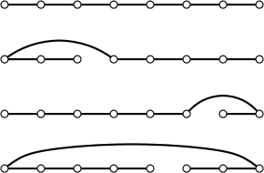
Figure 2: A path and three types of modification

Our most computationally challenging task was to find paths that realize each of approximately $6.4\times 10^{13}$ admissible multisets. For this a simple backtrack search is by far not efficient enough for large $n$, so we designed several improved algorithms. Here we describe the two most successful. Note that, although many special cases of Conjecture 1 have been proved, they are only a small fraction of cases for large $n$, so we chose to not exclude them from our search.

One observation used by both methods is this: if $k$ is an integer coprime to $n$, then $kM$ is realizable if and only if $M$ is realizable, where $kM=\{\mkern-3.0mu\{k\ell\bmod n\mid\ell\in M\}\mkern-3.0mu\}$. Thus, only one of the multisets in each equivalence class defined by this congruence need be tested.

One approach was a randomized form of hill-climbing. Figure 2 shows three ways to transform a path, which were employed for theoretical purposes by Horak and Rosa [6]. In each case, the induced multiset loses one element and gains another (perhaps equal). The idea is to start with some path and then repeatedly apply transformations until the required multiset is achieved.

Choice of transformation was made at random with a strong bias towards beneficial moves. Transformations which moved away from the target (fewer chords matched the required multiset) were given a weight of 1, sideways transformations (same number of matches) a weight of 100, and transformations that moved closer to the target had a weight of 10000 (or $\infty$ if the target multiset was immediately reached). The admissible multisets were processed in lexicographic order, meaning that each multiset was usually very similar to the one before. This meant it was efficient to use the solution for each multiset as the starting point to search for a solution for the following multiset.

There was a large limit on the number of iterations, with code to start over with a random path if the limit was reached, but this never happened. As an example, for $n=34$ the average number of iterations was $104$.

The second method for realizing multisets was a mixture of random and deterministic search. A boolean array indexed by a multiset ranking function kept track of which multisets had been realized, while simultaneously one process generated random paths and another realized multisets using a backtracking search. In both cases, multisets related by coprime multiplication (as described above) and by the last operation in Figure 2 were also marked off. The backtracking search had some problem-specific features that we now describe.

At each recursion level, we have a path so far, and a multiset of chord types that still need to be used. For each distinct chord type remaining, there can be 0, 1 or 2 unused points that can reached by such a chord. The order in which the possibilities are attempted is important for the average efficiency. When all possibilities are exhausted, backtrack to the previous level occurs.

Heuristics are used to try to guess at a good order in which to try chord types. In general, the program favors a pair of chord type and next point that leaves the next point with the fewest number of possible exits, and also favors chord types of which the fewest remain to be used. This all has much in common with the usual heuristics in backtracking Hamiltonian path solvers, including various conditions that allow to prune a search “early”.

There are also some specializations, driven by experience. For example, if $n$ is even, and only one instance of an odd chord type remains, there is only one possible place that chord can appear in the remaining path.

This usually worked very well, but in a small percentage of cases would take hundreds of times longer. A pleasant surprise was that Limited Discrepancy Search (LDS) [5], adapted for non-binary trees, proved extremely effective, 99.9% of the time finding a path with discrepancy no larger than 1, and with discrepancy 2 in 99% of the remaining cases. However, particularly for the largest size $n=28$ completed by this method, a handful of cases required discrepancies as high as 14 and took minutes of cpu time each.

For both implementations, whenever a realization is found it is checked in separate code. The result of the computations was that all admissible multisets for $n\leq 37$ are realizable. All cases for $n\leq 28$ were completed with both methods.

3 When two paths have the same length

For definiteness we will assume a circle of radius 1. The length of a chord of type $j$ is $2\sin(j\pi/n)$. Therefore, realizable multisets $[\ell_{1},\ldots,\ell_{m}]$ and $[\ell^{\prime}_{1},\ldots,\ell^{\prime}_{m}]$ have the same length if and only if $\sum_{j=1}^{m}(\ell^{\prime}_{j}-\ell_{j})\sin(j\pi/n)=0$. Also note that $\sum_{j=1}^{m}(\ell^{\prime}_{j}-\ell_{j})=0$, since all multisets in $\mathcal{M}_{n}$ have $n-1$ elements.

We will call a sequence $(a_{1},\ldots,a_{m})$ of rational numbers an identity if

$$\sum_{j=1}^{m}a_{j}\sin\Bigl{(}\frac{j\pi}{n}\Bigr{)} =0,\ \text{~{}~{}and}$$ (1)

$$\sum_{j=1}^{m}a_{j} =0.$$ (2)

Let $z=e^{i\pi/n}$, which is a primitive $(2n)$-th root of 1. Then $\sin\bigl{(}\frac{j\pi}{n}\bigr{)}=\lower 0.51663pt\hbox{\large$\textstyle\frac{1}{2i}$}(z^{j}-z^{-j})$. Thus (1) can be written

$$\frac{1}{2i}\sum_{j=1}^{m}a_{j}(z^{j}-z^{-j})=0.$$

Since $z\neq 0$, this is equivalent to $P_{n}(z)=0$, where

$$P_{n}(z)=z^{m}\sum_{j=1}^{m}a_{j}(z^{j}-z^{-j})=\sum_{j=1}^{m}a_{j}z^{m+j}-\sum_{j=1}^{m}a_{j}z^{m-j}.$$ (3)

Note that $P_{n}(z)$ is a polynomial with rational coefficients.

The cyclotomic polynomial of order $2n$ is the monic polynomial $\varPhi_{2n}(x)$ whose zeros are the primitive $(2n)$-th roots of unity. In particular, $\varPhi_{2n}(z)=0$. For the theory of cyclotomic polynomials, see Prasolov [13, pp. 89–99]. We will require these properties: (1) up to scaling, $\varPhi_{2n}(z)$ is the unique nonzero rational polynomial of least degree that has $z$ as a zero; (2) the degree of $\varPhi_{2n}(x)$ is Euler’s totient function $\varphi(2n)$ (the number of positive integers less than $2n$ and coprime to $2n$); (3) $\varPhi_{2n}(x)$ is palindromic (the list of coefficients reads the same forwards and backwards).

Perform a rational polynomial division:

$$P_{n}(x)=C_{n}(x)\varPhi_{2n}(x)+R_{n}(x),$$

where $C_{n}(x)$ is a rational polynomial and $R_{n}(x)$ has lower degree than $\varPhi_{2n}(x)$. Since $R_{n}(z)=0$, the minimality of $\varPhi_{2n}(x)$ implies that $R_{n}(x)$ is identically zero.

The coefficients of $R_{n}(x)$ are linear combinations of $a_{1},\ldots,a_{m}$ which must equal 0. Including equation (2), we have a linear system whose solution space is the vector space of all identities.

3.1 Example

Consider $n=15$, $m=7$. The cyclotomic polynomial is

$$\varPhi_{30}(x)=x^{8}+x^{7}-x^{5}-x^{4}-x^{3}+x+1.$$

Performing the division, we find $P_{15}(x)=C_{15}(x)\varPhi_{30}(x)+R_{15}(x)$, where

$$C_{15}(x) =a_{7}x^{6}+(a_{6}-a_{7})x^{5}+(a_{5}-a_{6}+a_{7})x^{4}+(a_{4}-a_{5}+a_{6})x^{3}$$

$${\qquad}+(a_{3}-a_{4}+a_{5})x^{2}+(a_{2}-a_{3}+a_{4}+a_{7})x+a_{1}-a_{2}+a_{3}+a_{6}-a_{7},$$

$$R_{15}(x) =(-a_{1}+a_{2}+a_{5}-a_{6}+a_{7})x^{7}+(-a_{1}+a_{2}+a_{4}+a_{7})x^{6}+(a_{1}-a_{2}+a_{3}+a_{6})x^{5}$$

$${\qquad}+(a_{1}-a_{3}+a_{6}-a_{7})x^{4}+(a_{1}-a_{2}-a_{4}-a_{7})x^{3}+(-a_{2}-2a_{5}-a_{7})x^{2}$$

$${\qquad}+(-a_{1}-a_{4}-2a_{6})x-a_{1}+a_{2}-a_{3}-a_{6}.$$

Now we require $R_{15}(x)=0$ identically, so we can set each of the coefficients to 0 and we also need $a_{1}+a_{2}+a_{3}+a_{4}+a_{5}+a_{6}+a_{7}=0$. In matrix form:

$$\begin{bmatrix}-1&1&-1&0&0&-1&0\\ -1&0&0&-1&0&-2&0\\ 0&-1&0&0&-2&0&-1\\ 1&-1&0&-1&0&0&-1\\ 1&0&-1&0&0&1&-1\\ 1&-1&1&0&0&1&0\\ -1&1&0&1&0&0&1\\ -1&1&0&0&1&-1&1\\ 1&1&1&1&1&1&1\end{bmatrix}\;\begin{bmatrix}a_{1}\\ a_{2}\\ a_{3}\\ a_{4}\\ a_{4}\\ a_{6}\\ a_{7}\end{bmatrix}=\begin{bmatrix}0\\ 0\\ 0\\ 0\\ 0\\ 0\\ 0\\ 0\\ 0\end{bmatrix}.$$

The solution space has dimension 2:

$$\bigl{\langle}(1,0,-1,-1,-1,0,2),(0,1,0,-2,-1,1,1)\bigr{\rangle}.$$

3.2 What is the dimension?

We now determine the dimension of the vector space of identities. For those values of $n$ where the dimension is 0, only paths with the same multiset of chord types have the same length.

Theorem 3.

For all $n\geq 1$, the dimension of the vector space of identities is

$$\max\bigl{\{}0,m-\tfrac{1}{2}\varphi(2n)-1\bigr{\}}.$$

In particular, the dimension is 0 if and only if $n=9$, or $n$ is a prime, twice a prime, or a power of 2.

Proof.

For a polynomial $f(x)=\sum_{j=0}^{k}b_{j}x^{j}$, we say that $f(x)$ is $k$-palindromic if $b_{k-j}=b_{j}$ for all $j$, and $k$-antipalindromic if $b_{k-j}=-b_{j}$ for all $j$. These properties are respectively equivalent to $x^{k}f(1/x)=f(x)$ and $x^{k}f(1/x)=-f(x)$. As examples, $\varPhi_{2n}(x)$ is $\varphi(2n)$-palindromic, while $P_{n}(x)$ defined in (3) is $2m$-antipalindromic.

Consider the equation $P_{n}(x)=C_{n}(x)\varPhi_{2n}(x)$. The degree of $C_{n}(x)$ is at most $t=2m-\varphi(2n)$. Note that $\varphi(2n)$ is even, so $t$ is also even. Also,

$$x^{t}C_{n}(1/x)=\frac{x^{2m}P_{n}(1/x)}{x^{\varphi(2n)}\varPhi_{2n}(1/x)}=\frac{-P_{n}(x)}{\varPhi_{2n}(x)}=-C_{n}(x),$$

so $C_{n}(x)$ is $t$-antipalindromic. By the same logic, if $C_{n}(x)$ is $t$-antipalindromic then $P_{n}(x)$ is $2m$-antipalindromic and so corresponds to a solution of (1).

Choosing a basis of $t/2$ linearly independent $t$-antipalindromic polynomials for $C_{n}(x)$, such as $x^{j}-x^{t-j}$ for $0\leq j\leq\frac{1}{2}t-1$, we find that the vector space of solutions of (1) has dimension $t/2$. If that vector space lies within the hyperplane defined by (2), the vector space of identities has dimension $t/2$; otherwise it has dimension $t/2-1$.

Recall that $\varphi(2n)=n\prod_{p}\,(1-1/p)$ where the product is over all distinct odd primes $p$ dividing $n$. From this, a little calculation shows that $t=0$ only if $n$ is an odd prime ($\varphi(2n)=n-1$) or a power of 2 ($\varphi(2n)=n$).

To show that the dimension is $t/2-1$ rather than $t/2$ when $t\geq 2$, we have only to find $(a_{1},\ldots,a_{m})$ that satisfies (1) but not (2). Let’s call this an improper identity.

Note that if $(a_{1},\ldots,a_{\lfloor n/2\rfloor})$ is an improper identity for $n$ then $(a^{\prime}_{1},\ldots,a^{\prime}_{\lfloor kn/2\rfloor})$ is an improper identity for $kn$, where $a^{\prime}_{kj}=a_{j}$ for $1\leq j\leq m$ and $a^{\prime}_{kj}=0$ otherwise. Therefore, it suffices to find improper identities for some values of $n$ that divide any value of $n$ giving $t\geq 2$. The minimum set is: twice an odd prime, the square of an odd prime, and the product of two distinct odd primes.

First, suppose that $n$ is twice an odd prime. Then $\varPhi_{2n}(x)=\sum_{j=0}^{n-1}(-1)^{j}x^{2j}$ and $t=2$. Taking $C_{n}(x)=x^{2}-1$, notice that the coefficients of $C_{n}(x)\varPhi_{2n}(x)$ are all $\pm 2$ except for the first and last which are $\pm 1$. Therefore, condition (2) is not satisfied and we have an improper identity.

Next suppose that $n=p^{2}$ where $p$ is an odd prime. Then $\varPhi_{2n}(x)=\sum_{j=0}^{p-1}x^{jp}$ and $t=p-1$. Consider $C_{n}(x)=x^{t/2-1}-x^{t/2+1}$, so $C_{n}(x)\varPhi_{2n}(x)=\sum_{j=0}^{p-1}\,(x^{jp+t/2-1}-x^{jp+t/2+1})$. The coefficients are thus in $\pm 1$ pairs, but for $j=(p-1)/2$ the pair is $x^{m-1}-x^{m+1}$. Thus, $\sum_{j=0}^{m}a_{j}$, which is the sum of the coefficients up to and including that of $x^{m-1}$, equals 1 and condition (2) is violated. So this is an improper identity.

Finally, consider $n=pq$ where $3\leq p<q$ are primes. Then $t=p+q-2$ and

$$\varPhi_{2n}(x)=\frac{(x+1)(x^{pq}+1)}{(x^{p}+1)(x^{q}+1)}.$$

Consider the $t$-antipalindromic polynomial $C_{n}(x)=x^{(q-3)/2}(x-1)(x^{p}+1)$. Then

$$C_{n}(x)\varPhi_{2n}(x)=\frac{x^{(q-3)/2}(x^{2}-1)(x^{pq}+1)}{x^{q}+1}=x^{(q-3)/2}(x^{2}-1)(x^{pq}+1)\sum_{j\geq 0}\,(-1)^{j}x^{jq}.$$

Since we are only interested in the coefficients up to $x^{m-1}$, we can ignore the factor $x^{pq}+1$, so the polynomial begins $\sum_{j\geq 0}(-1)^{j}(x^{jq+(q-3)/2+2}-x^{jq+(q-3)/2})$. The coefficients appear in $\pm 1$ pairs but for $j=(p-1)/2$ the pair is $\pm(x^{m-1}-x^{m+1})$. Thus the sum of coefficients up to that of $x^{m-1}$ is $\pm 1$ and this is an improper identity.

To complete the proof, note that $t/2-1=0$ in the case $t=2$, which occurs only for $n=9$ and twice an odd prime. ∎

The case of prime $n$ was previously noted by Simone Costa [1].

It is likely that the presence of an identity implies that there are two distinct realizable multisets with the same length, but this is something that remains open. It is plausible, if unlikely, that the constraints on realizability of multisets sometimes preclude the difference of two realizable multisets ever being an identity.

3.3 Generators

In this section we record generators for the vector spaces of identities. All cases for $n\leq 37$ which are not mentioned have dimension 0.

$n=12$

   [1, -2, 1, 0, -1, 1]

$n=15$

   [1, 0, -1, -1, -1, 0, 2]
   [0, 1,  0, -2, -1, 1, 1]

$n=18$

   [1, 0, -2, 0, 1, 0, -1,  0, 1]
   [0, 1, -2, 1, 0, 0,  0, -1, 1]

$n=20$

   [1, -2, 1, 0, -1, 2, -1, 0, 1, -1]

$n=21$

   [1, 0, 0, -1, -2,  0, 1, 1, 1, -1]
   [0, 1, 0, -1, -1, -1, 1, 2, 0, -1]
   [0, 0, 1,  0, -2, -1, 1, 2, 1, -2]

$n=24$

   [1, 0, 0, -2, 0, 0, 1, 0, -1,  0,  0, 1]
   [0, 1, 0, -2, 0, 1, 0, 0,  0, -1,  0, 1]
   [0, 0, 1, -2, 1, 0, 0, 0,  0,  0, -1, 1]

$n=25$

   [1, -1, -1, 1, 0, -1, 1, 1, -1, 0, 1, -1]

$n=27$

   [1, 0, 0, -1, -1, 0, 0, 1, 0, -1,  0,  0, 1]
   [0, 1, 0, -1, -1, 0, 1, 0, 0,  0, -1,  0, 1]
   [0, 0, 1, -1, -1, 1, 0, 0, 0,  0,  0, -1, 1]

$n=28$

   [1, -2, 1, 0, -1, 2, -1, 0, 1, -2, 1, 0, -1, 1]

$n=30$

   [1, 0, 0, 0, 0, 0, -2,  0, -1,  0, -1,  0, 2,  0, 1]
   [0, 1, 0, 0, 0, 0, -2,  1, -2,  0,  0, -1, 2,  0, 1]
   [0, 0, 1, 0, 0, 0, -1,  0, -2,  0,  0,  0, 1,  0, 1]
   [0, 0, 0, 1, 0, 0,  0, -2,  0, -1,  0,  1, 0,  1, 0]
   [0, 0, 0, 0, 1, 0, -1,  0, -1,  0,  0,  0, 1,  0, 0]
   [0, 0, 0, 0, 0, 1, -2,  2, -2,  1,  0, -1, 2, -2, 1]

$n=33$

   [1, 0, 0, 0, 0, -1, -2, -1, 1, 3, 1, -2, -2, -1, 1, 2]
   [0, 1, 0, 0, 0, -1, -2, -1, 2, 2, 1, -1, -3, -1, 1, 2]
   [0, 0, 1, 0, 0, -1, -2,  0, 1, 2, 1, -1, -2, -2, 1, 2]
   [0, 0, 0, 1, 0, -1, -1, -1, 1, 2, 1, -1, -2, -1, 0, 2]
   [0, 0, 0, 0, 1,  0, -2, -1, 1, 2, 1, -1, -2, -1, 1, 1]

$n=35$

   [1, 0, 0, 0, -1, -1, -1, -1,  0, 1, 2, 2, 1, 1,  0, -2, -2]
   [0, 1, 0, 0,  0, -2, -1,  0, -1, 1, 2, 1, 2, 1, -1, -1, -2]
   [0, 0, 1, 0, -1,  0, -1, -1,  1, 0, 0, 2, 1, 0,  0, -1, -1]
   [0, 0, 0, 1,  0, -2,  0,  1, -1, 0, 1, 0, 1, 1, -1, -1,  0]

$n=36$

   [1, 0, 0, 0, 0, -2, 0, 0, 0, 0, 1, 0, -1,  0,  0,  0,  0, 1]
   [0, 1, 0, 0, 0, -2, 0, 0, 0, 1, 0, 0,  0, -1,  0,  0,  0, 1]
   [0, 0, 1, 0, 0, -2, 0, 0, 1, 0, 0, 0,  0,  0, -1,  0,  0, 1]
   [0, 0, 0, 1, 0, -2, 0, 1, 0, 0, 0, 0,  0,  0,  0, -1,  0, 1]
   [0, 0, 0, 0, 1, -2, 1, 0, 0, 0, 0, 0,  0,  0,  0,  0, -1, 1]

4 Counting distinct lengths

Having verified that the realizable multisets are the admissible multisets for $n\leq 37$, our next task is to determine how many distinct lengths occur for the admissible multisets.

One way is to compute accurate numerical approximations for the lengths, sort them, then rigorously verify equality for those lengths which are no further apart than rounding error can explain. We carried this out up to $n=28$ but memory limits prevented us from going further. This led us to a better method.

For a multiset $M\in\mathcal{A}_{n}$, let $\mathcal{L}(M)$ be the set of all multisets in $\mathcal{A}_{n}$ that have the same length as $M$, including $M$ itself. A multiset $M$ is minimal if it is lexicographically least in $\mathcal{L}(M)$. Since each set $\mathcal{L}(M)$ has exactly one minimal element, we have that the number of distinct lengths equals the number of minimal admissible multisets.

The task is thus reduced to recognizing minimal multisets. Recall that admissible multisets $M,M^{\prime}$ have the same length if and only if $M-M^{\prime}$ is an identity. So, if $M+A$ is an admissible multiset for some nonzero identity $A$ whose first nonzero entry is negative, then $M$ is not minimal. We will say that $A$ eliminates $M$. If there is no such $A$ for which $M+A$ is an admissible multiset, then $M$ is minimal.

The number of identities to test is reduced to a finite number by noting that $M+A$ has at least one negative entry if some subset of entries in $A$ has sum greater than $n-1$. However, in practice there are too many identities remaining. For $n=30$ there are 1,552,732 identities and 78,356,395,953 admissible multisets; the combination is infeasible. For $n=36$ the situation is even worse: 214,302 identities and 21,944,254,861,680 admissible multisets. Fortunately we do not need to test so many identities.

For a multiset or identity $X$, and $2\leq d\leq m$, let $\varSigma_{d}(X)$ be the sum of the entries of $X$ whose position is divisible by $d$. Recall that the definition of admissibility of a multiset $M$ is that $\varSigma_{d}(M)\leq n-d$ whenever $d$ is a divisor of $n$.

For identities $A=(a_{1},\ldots,a_{m})$ and $B=(b_{1},\ldots,b_{m})$ write $B\rightarrowtail A$ if the following two conditions are satisfied.
(a) For $1\leq j\leq m$, either $a_{j}\geq 0$ or $a_{j}\geq b_{j}$.
(b) For each divisor $d$ of $n$, either $\varSigma_{d}(A)\leq 0$ or $\varSigma_{d}(A)\leq\varSigma_{d}(B)$.

Lemma 4.

Let $A,B$ be identities with $B\rightarrowtail A$. Then if $B$ eliminates admissible multiset $M$, so does $A$.

Proof.

Let $M=[\ell_{1},\ldots,\ell_{m}]$, $A=(a_{1},\ldots,a_{m})$ and $B=(b_{1},\ldots,b_{m})$. We are given that $M$ and $M+B$ are admissible multisets, and need to show that $M+A$ is also an admissible multiset.

For $1\leq j\leq m$, if $a_{j}\geq 0$ then $\ell_{j}+a_{j}\geq\ell_{j}\geq 0$, whereas if $a_{j}\geq b_{j}$ then $\ell_{j}+a_{j}\geq\ell_{j}+b_{j}\geq 0$. So $M+A$ is nonnegative, i.e., is a multiset.

For divisor $d$ of $n$, if $\varSigma_{d}(A)\leq 0$ then $\varSigma_{d}(M+A)\leq\varSigma_{d}(M)\leq n-d$, whereas if $\varSigma_{d}(A)\leq\varSigma_{d}(B)$ then $\varSigma_{d}(M+A)\leq\varSigma_{d}(M+B)\leq n-d$. So $M+A$ is admissible. This completes the proof. ∎

Lemma 4 is surprisingly powerful. Start with all identities whose first nonzero entry is negative and such that no subset of the entries sums to greater than $n-1$. Then repeatedly remove identities $B$ from the set if there is a different identity $A$ still in the set such that $B\rightarrowtail A$. At each stage, Lemma 4 guarantees that the ability to eliminate multisets is maintained. For $n=30$, the number of required identities is reduced from 1,552,732 to $65$. The count for each $n$ is shown in the last column of Table 1.

$n$	$\mathopen{|}\mathcal{M}_{n}\mathclose{|}$	$\mathopen{|}\mathcal{R}_{n}\mathclose{|}=\mathopen{|}\mathcal{A}_{n}\mathclose{|}$	distinct lengths	Dimen	Essential
3	1	1	1
4	4	3	3
5	5	5	5
6	21	17	17
7	28	28	28
8	120	105	105
9	165	161	161
10	715	670	670
11	1001	1001	1001
12	4368	4129	2869	1	1
13	6188	6188	6188
14	27132	26565	26565
15	38760	38591	14502	2	4
16	170544	167898	167898
17	245157	245157	245157
18	1081575	1072730	445507	2	3
19	1562275	1562275	1562275
20	6906900	6871780	6055315	1	1
21	10015005	10011302	2571120	3	7
22	44352165	44247137	44247137
23	64512240	64512240	64512240
24	286097760	285599304	65610820	3	6
25	417225900	417219530	362592230	1	1
26	1852482996	1850988412	1850988412
27	2707475148	2707392498	591652989	3	6
28	12033222880	12026818454	11453679146	1	1
29	17620076360	17620076360	17620076360
30	78378960360	78356395953	1511122441	6	65
31	114955808528	114955808528	114955808528
32	511738760544	511647729284	511647729284
33	751616304549	751614362180	67876359922	5	40
34	3348108992991	3347789809236	3347789809236
35	4923689695575	4923688862065	1882352047787	4	32
36	21945588357420	21944254861680	1404030562068	5	17
37	32308782859535	32308782859535	32308782859535

Table 1: Counts of realizable multisets and the number of distinct lengths. “Dimen” is the dimension of the vector space of identities and “Essential” is the number of identities required in Section 4. For readability, zeros in the last two columns are left blank.

$n$	$\mathopen{|}\mathcal{M}_{n}\mathclose{|}$	$\mathopen{|}\mathcal{A}_{n}\mathclose{|}$
38 38	144079707346575	144074954225730
39 39	212327989773900	212327943155328
40 40	947309492837400	947290091984737
41 41	1397281501935165	1397281501935165
42 42	6236646703759395	6236574886430483
43 43	9206478467454345	9206478467454345
44 44	41107996877935680	41107708028136365
45 45	60727722660586800	60727721456103761
46 46	271250494550621040	271249413252489750
47 47	400978991944396320	400978991944396320
48 48	1791608261879217600	1791603906671596709
49 49	2650087220696342700	2650087220630545150
50 50	11844267374132633700	11844250906909678730

Table 2: Counts of admissible multisets. These have not been shown to be realizable.

5 Results

By elementary combinatorics, $\mathopen{|}\mathcal{M}_{n}\mathclose{|}=\binom{n+m-2}{m-1}$. The size of $\mathcal{A}_{n}$ has no formula that we know of, but it is easy to compute for small $n$.

The most expensive task was the verification that $\mathcal{R}_{n}=\mathcal{A}_{n}$ for $n\leq 37$, which took approximately four years of cpu time. By contrast, counting distinct lengths took only about 500 hours.

While the authors shared ideas, in the interest of establishing independent reproducibility they did not share code, hardware, or even programming languages. All of the computations were completed independently by the two authors except for the very expensive realization of admissible multisets for $29\leq n\leq 37$.

The counts resulting from our computations are shown in Table 1. Additional values of $\mathopen{|}\mathcal{A}_{n}\mathclose{|}$, which took less than one minute to compute, are given in Table 2. Note that these additional admissible multisets have not been tested for realizability.

The average testing time per multiset generally grew at a slower rate than the number of multisets, so the latter is the main indicator for how expensive it would be to extend the computation to larger sizes. We also observed that realizability testing tended to be more difficult if $n$ is highly composite, compared to prime or near-prime.

6 OEIS sequences

This paper extends the following entries in the Online Encyclopedia of Integer Sequences.

A030077  Take $n$ equally spaced points on circle, connect them by a path with $n-1$ line segments; sequence gives number of distinct path lengths.

A352568  Take $n$ equally spaced points on circle, connect them by a path with $n-1$ line segments; sequence gives number of distinct multisets of segment lengths.

References

- [1] M. Buratti, personal communication, May 2022.
- [2] S. Capparelli and A. Del Fra, Hamiltonian paths in the complete graph with edge-lengths 1, 2, 3, Electron. J. Combin. 17 (2010), #R44.
- [3] P. Chand and M. A. Ollis, The Buratti–Horak–Rosa conjecture holds for some underlying sets of size three, preprint, 2022, https://arxiv.org/abs/2202.07733.
- [4] D. L. Gittelson, personal communication, June 2022.
- [5] W. D. Harvey and M. L. Ginsberg, Limited Discrepancy Search, IJCAI’95: Proceedings of the 14th international joint conference on Artificial intelligence, vol. 1, Aug. 1995, 607–613.
- [6] P. Horak and A. Rosa, On a problem of Marco Buratti, Electron. J. Combin. 16 (2009), #R20.
- [7] M. Meszka, Private communication to Horak and Rosa [6].
- [8] T. E. Noe, Contribution to OEIS sequence A030077, 2007, https://oeis.org/A030077.
- [9] M. A. Ollis, A. Pasotti, M. A. Pellegrini, and J. R. Schmitt, New methods to attack the Buratti–Horak–Rosa conjecture, Discrete Math. 344 (2021) 112486.
- [10] M. A. Ollis, A. Pasotti, M. A. Pellegrini, and J. R. Schmitt, Growable realizations: a powerful approach to the Buratti–Horak–Rosa conjecture, Ars Math. Contemp. 22 (2022) #P4.04.
- [11] A. Pasotti and M. A. Pellegrini, A new result on the problem of Buratti, Horak and Rosa, Discrete Math. 319 (2014) 1–14.
- [12] A. Pasotti and M. A Pellegrini, On the Buratti–Horak–Rosa conjecture about Hamiltonian paths in complete graphs, Electron. J. Combin. 21 (2014), #P2.30.
- [13] V. Pasolov (trans. D. Leites), Polynomials, Springer-Verlag, Berlin, 2004.
- [14] A. Vázquez-Ávila, A note on the Buratti–Horak–Roza conjecture about hamiltonian paths in complete graphs, Bull. Inst. Combin. Appl. 94 (2022) 53–70.