The role of investor attention in global asset price variation during the invasion of Ukraine

Abstract

We study the impact of event-specific attention indices – based on Google Trends – in predictive price variation models before and during the Russian invasion of Ukraine in February 2022. We extend our analyses to the importance of geographical proximity and economic openness to Russia within 51 global equity markets. Our results demonstrate that 36 countries show significant attention to the conflict at the onset of and during the invasion, which helps predict volatility. We find that the impact of attention is more significant in countries with a higher degree of economic openness to Russia and those nearer to it.

[inst1]organization=Department of Finance, The Faculty of Economics and Administration, Masaryk University,addressline=Lipova 41a, city=Brno, postcode=60200, country=Czech Republic

1 Introduction

The prelude to the Russo–Ukrainian war began in mid-October 2021, during which Russian forces gathered near Ukraine’s borders and in the occupied Crimea region (Lister, 2021). Shortly thereafter, aggressive and escalating statements from Russian policymakers were reported (Bowen, 2022), which led Joe Biden to announce consequences in the event of any Russian invasion of Ukraine (Shalal et al., 2021). As a result (on December 8), we observe the first sharp growth in the conflict attention index depicted in Figure 1, meaning that this threat was likely recognized by many. The intelligence provided by Western security agencies suggested that a possible Russian invasion could start in early 2022 (Harris and Sonne, 2021). Considering those warnings, combined with the growth of tensions, military movements (Salama et al., 2022), and accusations (Olearchyk et al., 2022), the attention paid to the possible conflict grew rapidly.

Figure 1: Conflict attention index and daily price volatility on four continents

Notes: The daily volatility for each area is computed as an average of the individual volatilities of available Morgan Stanley Capital International (MSCI) indices for the particular area. Furthermore, for the Americas volatility average, we used both the North and South American MSCI indices. The vertical red dashed line divides the time series into two periods. We label them the pre-invasion and onset-of-invasion periods.

In his speech on February 21, 2022, President Putin announced that Russia had recognized the separatist republics in eastern Ukraine, which was followed by consequent threats to Ukraine (Reuters, 2022a). In the early morning of February 24, Russian armed forces began a full-scale war against Ukraine.

The response was to impose unprecedented economic sanctions on the Russian economy, which were implemented shortly after the invasion and targeted all kinds of industries such as banking, oil exports, and high-tech components. However, due to economic interconnectedness and dependency on Russian commodities, those sanctions also created risks for all companies and households in countries economically linked to Russia. The sanctions are already resulting in recognizable economic consequences, especially for Europe, whose largest energy supplier is Russia (in 2021, approximately 45% of imported natural gas came from Russia (IEA, 2022)). Along with a sharp increase in energy prices, we are also witnessing devastating consequences for countries that rely on Ukrainian wheat imports (Simon and Davies, 2022). Thus, this war has evolved into a serious global economic and political issue that is subject to exceptional worldwide attention.

In this context, our aim is to investigate this extraordinary interest and determine whether it is linked to increased volatility of stock markets around the globe. We build upon a growing literature related to the relationship between future market movements and investor behavior, particularly investor sentiment and investor attention.

From a theoretical perspective, we rely on the limited attention hypothesis of Barber and Odean (2008), according to which investors face a difficult task of choosing among numerous investment opportunities, despite possessing limited time and resources, and thus gravitate toward ”attention-grabbing” options. Andrei and Hasler (2015) expand on this idea to demonstrate that news that receives substantial interest takes less time to be incorporated into prices. Their results also suggest that investors seek more information during times of high uncertainty – such as the unexpected Russian military invasion of Ukraine.

To capture investors’ panic, fear, and uncertainty, we use a very popular direct measure of attention, the Google Search Volume Index (SVI). Some of the first applications of Google query data in research came from epidemiology (Ginsberg et al., 2009; Dugas et al., 2013); however, such approaches rapidly spread to the field of finance (Da et al., 2011; Joseph et al., 2011) as a proxy for attention (albeit sometimes imprecisely referred to as a sentiment proxy). Search volume has been shown to be correlated with lagged trading volumes (Preis et al., 2010; Bordino et al., 2012), to improve trading strategies (Preis et al., 2013; Bijl et al., 2016) or diversification strategies (Kristoufek, 2013). For economic mechanisms explaining how the attention may impact future volatility, refer, for example, to Aouadi et al. (2013); Vlastakis and Markellos (2012); Hamid and Heiden (2015); Dimpfl and Jank (2016); Audrino et al. (2020). Several studies have also examined interest in cryptocurrencies, measured with Google, as a driver of their price and volume fluctuations (Kristoufek, 2013, 2015; Garcia et al., 2014; Cheah and Fry, 2015; Cretarola et al., 2020; Urquhart, 2018; Aalborg et al., 2019; Eom et al., 2019; Burggraf et al., 2020; Chen et al., 2020). Similar results can be found for major FX markets (Kita and Wang, 2012; Smith, 2012; Goddard et al., 2015; Han et al., 2018; Wu et al., 2019; Saxena and Chakraborty, 2020; Kapounek et al., 2021).

Investor attention appears to be particularly effective in studies related to specific events, which is also the case for our study, namely attention devoted to macroeconomic developments (Lyócsa et al., 2020b; Plíhal, 2021), earnings news announcements (Hirshleifer et al., 2011; Hirshleifer and Sheng, 2021; Fricke et al., 2014; Ben-Rephael et al., 2017), the outbreak of the COVID-19 pandemic (Chen et al., 2020; Lyócsa et al., 2020a), and even this military conflict (Lyócsa and Plíhal, 2022).

We contribute to this literature on the impact of event-specific attention by exploring the one-day ahead predictive power of investor attention devoted to the military conflict in Ukraine in volatility models. We divide the data into two samples (the pre-invasion and onset-of-invasion periods) to compare the effects of such attention on price fluctuations. The analysis covers the stock indices of 51 countries. Our goal is to compare these results and determine whether (1) geographical or (2) economic proximity to the conflict influences the impact of conflict attention on volatility.

The remainder of this paper is organized as follows. In section 2, we describe the data, their sources, and how they were processed into the measures used for analysis. In the following section 3, we present and describe the results and emphasize their place in the context of the war and economic connectedness. Finally, we conclude by describing our results and contributions.

2 Data and methodology

2.1 Financial data

Our financial data consist of two datasets – the daily prices of selected indices and economic indicators. The first dataset includes data from all countries with an available MSCI index. MSCI indices were selected because of the consistent methodology used to calculate indices for all included countries. In addition to the MSCI indices, we include the Latvian stock index – OMX Riga – to capture the impact in this Baltic state. The data were collected from a Bloomberg terminal as an OHLC dataset. After removing countries with missing OHL observations, our sample covers 51 countries, including 8 regions in the Americas, 3 regions in Africa, 19 European countries, and 21 Asia-Pacific regions, including Australia. The period of study is from June 22, 2021, to March 8, 2022. For modeling purposes, the dataset was divided into two periods – before the invasion of Ukraine, June 22, 2021, to December 31, 2021, and during the onset of the invasion of Ukraine from January 1, 2022, to March 8, 2022. The median number of observations in the pre-invasion and onset-of-invasion samples is 136 and 47, respectively.

The second financial dataset considers a filtered set of countries based on previously mentioned conditions. For each country, we extracted data on imports from Russia and exports to Russia, as well as GDP, all for the year 2020. The source of these data is the UN Comtrade Database. This dataset was used to calculate the degree of openness (DOO) (Rodriguez, 2000) to Russia of country $i$ country as follows:

$$DOO_{i}=\frac{Export_{i}+Import_{i}}{GDP_{i}},$$ (1)

where $GDP_{i}$ is the GDP of country $i$, $Export_{i}$ is the exports of country $i$ to Russia and $Import_{i}$ is the imports of country $i$ from Russia. In addition, we define a variable $Dist_{i}$, as a distance to Moscow from $ith$ country capital. The distance is measured in the order of $10^{3}km$.

2.2 Attention measures

Our attention measures were retrieved from Google Trends with the help of the R package gtrendsR (Massicotte and Eddelbuettel, 2021). Unfortunately, the availability of daily data is limited to 270-day intervals, and longer samples would require additional scaling. Although this may appear to be a relatively short sample, we opt for the 270-day interval, as it sufficiently covers the events we want to consider. Previous literature points to the presence of seasonality in attention. Thus, if our sample was larger, we could use fixed effects to address this issue (Liu et al., 2021).

We use two sets of search terms to construct two variables, one related to general stock market attention and one for the attention paid to the military conflict, denoted $G_{t}$ and $C_{t}$, respectively. We include the general index to ensure that we measure the effect of excess attention to the conflict adjusted for the general day-to-day interest of investors in trading. Since we sought to capture global interest, we opted for queries of topics – an option that automatically translates keywords into all available languages and accounts for spelling variations. We primarily wanted to aim our research at international investors, as the developed financial markets are very tied to each other, reflecting the global macroeconomic shocks and unprecedented events such as this one. Thus we decided to retrieve the data using the ”worldwide” option. The $G_{t}$ and $C_{t}$ indices are then adjusted for the time zones of the stock exchanges corresponding to each MSCI index in our dataset. For the MSCI indices that cover more than one country, we select the time zone with the majority coverage, as reported in the country weights in the MSCI fact sheets. Table 1 provides summary statistics for indices $G_{t}$ and $C_{t}$ after log transformation in three different time zones.

After accounting for time zones, we also remove values for nontrading days. Our approach consists of taking the maximum value of Friday to Sunday and assigning this value to Friday, and the method is applied for holidays. This procedure must be applied individually to each country, as the nontrading days are not identical.

Table 1: Descriptive statistics of variables of conflict and general attention indeces

	Mean	S.D.	Median	Min.	Max.	$\rho(1)$	$\rho(5)$
$C_{t}$ (UTC+0)	0.453	0.936	0.182	-0.916	4.605	0.944	0.796
$C_{t}$ (UTC+6)	0.549	0.912	0.223	-0.693	4.605	0.940	0.809
$C_{t}$ (UTC-6)	0.452	0.937	0.182	-0.916	4.605	0.943	0.797
$G_{t}$ (UTC+0)	3.862	0.147	3.861	3.188	4.178	0.609	0.410
$G_{t}$ (UTC+6)	3.862	0.149	3.861	3.188	4.178	0.630	0.458
$G_{t}$ (UTC-6)	3.860	0.148	3.856	3.188	4.177	0.629	0.430

Notes: S.D. stands for standard deviation, $\rho(1)$ represents the first-order autocorrelation coefficient and $\rho(5)$ denotes the fifth-order autocorrelation.

We used five topic search terms to create the conflict index $C_{t}$ (’Russia’, ’Ukraine’, ’Vladimir Putin’, ’NATO’, and ’sanctions’) and 31 topics A to construct the general attention index $G_{t}$. We based our general topic selection on previous studies that captured general attention via a list of financial keywords. In particular, our list of topics closely resembles keywords used by Mao et al. (2011); Preis et al. (2013). In addition, our initial list of search words was first reduced to those keywords that could be obtained as Google topics. Furthermore, to ensure that the resulting average $G_{t}$ variable captures one common phenomenon, we prune the list of keywords by removing topics whose SVI is negatively correlated with the rest of the topics. From previous experience working with attention measures in volatility forecasting, this usually helps remove noise from the data.

Both attention indices are then calculated as simple averages of the individual variables. These data take the form of a normalized volume ratio on a scale of 0–100, where 100 represents the maximum search activity during the selected period. The acquired search volume ratio $SVI_{t}$ at time $t$ can be further transformed according to the procedure proposed by Da et al. (2011) into the abnormal search volume index ($ASVI_{t}$), which should help us to identify significant changes in Google searches.

The $ASVI_{t}$ is usually applied to address the noisiness of $SVI_{t}$ and to capture only abnormal search activity. However, it does not capture the scale of the abnormal change. As the data we are working with have a rather unusual shape, with nearly exponential growth around the time of the invasion of Ukraine, we concluded that the $ASVI_{t}$ transformation is not suitable for our analysis. Instead, we opt for a log transformation of $SVI_{t}$. For the remainder of the paper we use $G_{t}$ and $C_{t}$ in this log-transformed form.

2.3 Price variation estimator

As we rely on MSCI indices, we are limited to the use of daily OHLC data, which do not allow us to use the standard realized volatility estimator calculated as the sum of squared intraday returns (see, e.g., Andersen et al. (2003)). Thus, to maintain the stylized facts of the volatility time series, we employ a range-based volatility estimator following the approach of Lyócsa et al. (2021), which was originally motivated by the approach of Patton and Sheppard (2009), who notes that since the true data generating process is unknown, the optimal estimator must also be unknown. Therefore, a combination of several estimators may be less prone to estimator choice uncertainty:

$$V_{t}=100^{2}\times(J_{t}+3^{-1}(PK_{t}+GK_{t}+RS_{t}))$$ (2)

where $V_{t}$ is the price variation estimator. Furthermore, for every day $t=1,2,...,T$, we compute the average of three different realized range-based estimators ($PK_{t}$, $GK_{t}$, $RS_{t}$) and adjust the final price variation estimates for overnight price variation $J_{t}$. We denote by $PK_{t}$ the estimator of Parkinson (1980):

$$PK_{t}=\frac{(h_{t}-l_{t})^{2}}{4\ln 2}$$ (3)

by $GK_{t}$ the volatility estimator of Garman and Klass (1980) is defined as:

$$GK_{t}=0.511(h_{t}-l_{t})^{2}-0.019(c_{t}(h_{t}+l_{t})-2h_{t}l_{t})-0.383c_{t}^{2}$$ (4)

by $RS_{t}$ the Rogers and Satchell (1991) estimator takes the form:

$$RS_{t}=h_{t}(h_{t}-c_{t})+l_{t}(l_{t}-c_{t})$$ (5)

and finally, the overnight price variation is defined as:

$$J_{t}=[\ln(Open_{t})-\ln(Close_{t-1})]^{2}$$ (6)

where $Open_{t}$, $High_{t}$, $Low_{t}$, and $Close_{t}$ represent the open, high, low and close prices on a given day $t$. Furthermore, define $h_{t}=\ln(High_{t})-\ln(Open_{t})$, $l_{t}=\ln(Low_{t})-\ln(Open_{t})$, $c_{t}=\ln(Close_{t})-\ln(Open_{t})$.

The estimated daily volatilities are in 8.

2.4 Model specification

With a focus on the attention variables and subsequent exploration of their impact on price variation, we define a parsimonious model, mimicking the well-known and time-tested heterogeneous autoregressive (HAR-RV) model of Corsi (2009). By doing so, we investigate whether the attention to the invasion of Ukraine prompted individual investors to increase their trading activities, which would raise volatility. In contrast to the standard HAR-RV, we omit the monthly component because, as presented in Table 8, the fifth-order autocorrelation is low in some cases. During our main period of interest, the uncertainty about subsequent price developments is so high that what the last month’s price variation was should rarely matter.

$$V_{t+1}=\beta_{0}+\beta_{1}V_{t}+\beta_{2}V_{t}^{w}+\beta_{3}C_{t}+\beta_{4}G_{t}+\epsilon_{t+1}$$ (7)

where $C_{t}$ and $G_{t}$ are the attention variables defined in the previous section. $V_{t}^{w}$ is the weekly price variation component given as $V_{t}^{w}=5^{-1}\sum_{j=0}^{4}V_{t-j}$. The model in Equation 7 is estimated via ordinary least squares and for both data samples, that is, in the pre-invasion and onset-of-invasion periods. Next, we estimate the model with the log-transformed price variation.

In order to test the significance of attention variables across the worldwide indices and also hypotheses developed further in the results section, we opted to utilize panel data regression models, defined as:

$$V_{i,t+1}=\beta_{0}+\beta_{1}V_{i,t}+\beta_{2}V_{i,t}^{w}+\beta_{3}C_{i,t}+\beta_{4}G_{i,t}+\alpha_{i}+\epsilon_{i,t+1}$$ (8)

$$V_{i,t+1}=\beta_{0}+\beta_{1}V_{i,t}+\beta_{2}V_{i,t}^{w}+\beta_{3}C_{i,t}+\beta_{4}G_{i,t}+\beta_{5}C_{i,t}X_{i}+\alpha_{i}+\epsilon_{i,t+1}$$ (9)

where e.g. $V_{i,t}$ is volatility of $ith$ cross-sectional unit at time $t$, $\alpha_{i}$ is the unobserved heterogeneity and $X_{i}$ stands for either the $DOO_{i}$ or $Dist_{i}$. We estimate the model parameters via fixed effect panel data regression with standard error of Driscoll and Kraay (1998) robust to cross-sectional and temporal dependence. Hence, we name the Equation 8 as FE-DK model and Equation 9 FE-DK-DOO and FE-DK-Dist.

3 Results

Firstly, we explore the significance of the independent variables across all 51 countries via estimating Equation 8. As presented in Table 2, in the pre-invasion period all regressors, except the conflict attention variable are significant, which is to be expected. In contrast, within the onset-of-invasion period, the $C_{t}$ is among the most significant, explaining high portion of the model variability. This may point to a partial conclusion, that in the onset-of-invasion period, the conflict attention is important in explaining day-ahead volatility throughout all of the indices. However, this may not hold for individual countries.

Table 2: Exploration of the significance of attention variables across all market indices

	FE-DK-pre	FE-DK-during
$const$	$\textbf{-2.572}^{b}$	$\textbf{-3.091}^{a}$
$V_{i,t}$	$\textbf{0.158}^{d}$	$\textbf{0.196}^{c}$
$V^{w}_{i,t}$	$\textbf{0.326}^{d}$	$0.167$
$C_{i,t}$	$-0.056$	$\textbf{0.245}^{d}$
$G_{i,t}$	$\textbf{0.578}^{b}$	$0.704$
$R^{2}(within)$	0.109	0.231
$R^{2}(between)$	0.728	0.579
$F-statistic$	203.721	162.120

Notes: FE-DK-pre is the Equation 8 estimated on the pre-invasion data sample, whereas FE-DK-during is estimated on the onset-of-invasion sample. Superscripts $a$, $b$, $c$ and $d$ denote statistical significance of estimated coefficients at the 10%, 5%, 1% and 0.1% level.

Therefore, we estimate the model defined in Equation 7 for all 51 stock market indices for both the before the invasion and onset-of-invasion periods. The results show that in 70% of countries, the conflict attention variable $C_{t}$ has a significant positive effect on future volatility. In other words, the more common military conflict topic searches are, as measured by Google searches, the higher the next day’s volatility of MSCI indices. Table 3 then presents estimates and diagnostics for those indices for which we found the most significant impact of conflict attention, while Table 4 shows the least significant impacts. The parameter estimates of the remaining countries are reported in the Appendix in Table 6 and Table 7. Each table also compares the results for the sample before the invasion of Ukraine (Panel B) and during the onset of the invasion (Panel A).

Table 3: Results with the most significant conflict attention variable $C_{t}$

	Poland	Denmark	Czechia	Great Britain	Portugal	Hungary	Belgium	Greece	Finland	Italy
Panel A: OLS parameters estimates - with the most significant $C_{t}$
Constant	1.764	$\textbf{-4.505}^{a}$	-0.597	-3.809	-2.885	3.725	$\textbf{-4.965}^{a}$	1.353	-3.579	-4.192
$V_{t}$	0.033	-0.093	0.252	0.129	0.200	0.139	0.040	0.013	0.057	0.150
$V_{w}$	$\textbf{-0.632}^{d}$	$\textbf{-0.822}^{c}$	-0.161	0.040	$\textbf{-0.460}^{b}$	0.215	-0.127	-0.122	0.012	-0.005
$C_{t}$	$\textbf{1.198}^{d}$	$\textbf{0.715}^{d}$	$\textbf{0.782}^{d}$	$\textbf{0.504}^{d}$	$\textbf{0.684}^{d}$	$\textbf{0.703}^{d}$	$\textbf{0.723}^{d}$	$\textbf{0.653}^{d}$	$\textbf{0.618}^{d}$	$\textbf{0.652}^{d}$
$G_{t}$	-0.569	$\textbf{1.329}^{b}$	-0.230	0.654	0.677	-1.036	1.038	-0.515	0.801	0.876
Panel A1: Estimated models diagnostics
$R^{2}$	0.788	0.486	0.686	0.570	0.668	0.756	0.642	0.499	0.614	0.586
$adj.R^{2}$	0.767	0.436	0.656	0.527	0.636	0.733	0.607	0.448	0.575	0.546
residual $\rho(1)$	0.112	0.144	0.066	0.032	0.124	-0.036	0.083	0.040	0.093	0.050
Ljung-Box	0.491	0.854	0.419	0.926	0.702	0.036	0.197	0.010	0.642	0.283
White	0.612	0.950	0.840	0.889	0.202	0.772	0.828	0.777	0.559	0.122
Panel B: Parameters estimates of the same model using pre-invasion data sample
Constant	$\textbf{-5.279}^{c}$	$\textbf{-3.590}^{b}$	$\textbf{-4.859}^{c}$	-2.337	$\textbf{-3.400}^{a}$	-3.071	-2.047	-1.444	$\textbf{-4.604}^{b}$	-0.479
$V_{t}$	0.030	$\textbf{0.313}^{d}$	$\textbf{0.395}^{d}$	0.123	0.085	$\textbf{0.227}^{b}$	0.138	0.130	0.001	$\textbf{0.262}^{c}$
$V_{w}$	$\textbf{0.541}^{d}$	0.147	0.079	$\textbf{0.292}^{a}$	0.210	$\textbf{0.365}^{b}$	0.163	0.029	$\textbf{0.532}^{d}$	0.181
$C_{t}$	-0.173	-0.313	0.217	0.067	0.075	0.057	0.098	-0.208	-0.240	-0.028
$G_{t}$	$\textbf{1.311}^{b}$	$\textbf{0.896}^{b}$	$\textbf{1.142}^{b}$	0.388	$\textbf{0.830}^{a}$	0.766	0.357	0.286	$\textbf{1.087}^{a}$	-0.016
Panel B1: Estimated models diagnostics
$R^{2}$	0.249	0.185	0.263	0.076	0.080	0.227	0.059	0.028	0.176	0.119
$adj.R^{2}$	0.226	0.160	0.240	0.048	0.053	0.203	0.031	-0.002	0.151	0.093
residual $\rho(1)$	0.004	-0.017	-0.050	0.013	0.020	-0.017	0.009	0.014	-0.000	-0.024
Ljung-Box	0.584	0.793	0.750	0.207	0.176	0.994	0.567	0.489	0.556	0.948
White	0.214	0.086	0.558	0.181	0.109	0.302	0.044	0.931	0.009	0.384

Notes: In the header, we use ISO 3166 country codes. Regression parameter estimates in bold indicate significance at the 10% level; superscripts $a$, $b$, $c$ and $d$ denote statistical significance of estimated coefficients at the 10%, 5%, 1% and 0.1% level. Residuals $\rho(1)$ describe the first-order autocorrelation of the residuals. For the Ljung-Box and White tests, we report the corresponding p-values.

Table 4: Results with the least significant conflict attention variable $C_{t}$

	Brazil	Jordan	Argentina	Korea	Philippines	Taiwan	Japan	Columbia	Canada	Peru
Panel A: OLS parameters estimates - with the least significant $C_{t}$
Constant	$\textbf{-12.904}^{a}$	-8.610	$\textbf{-11.535}^{c}$	-1.054	1.189	$\textbf{-6.584}^{b}$	0.834	-5.844	$\textbf{-13.732}^{d}$	$\textbf{-11.051}^{c}$
$V_{t}$	0.115	0.131	0.191	0.110	0.267	-0.065	0.090	0.002	$\textbf{0.281}^{a}$	0.089
$V_{t}^{w}$	-1.110	-0.155	-0.152	0.187	-0.166	$\textbf{-0.824}^{c}$	0.211	0.360	-0.071	-0.001
$C_{t}$	-0.784	0.175	0.106	0.096	0.116	-0.066	0.087	0.075	0.021	-0.012
$G_{t}$	$\textbf{3.898}^{a}$	1.990	$\textbf{3.252}^{d}$	0.197	-0.424	$\textbf{1.599}^{b}$	-0.265	1.493	$\textbf{3.373}^{d}$	$\textbf{3.018}^{c}$
Panel A1: Estimated models diagnostics
$R^{2}$	0.097	0.136	0.283	0.102	0.079	0.197	0.059	0.040	0.386	0.197
$adj.R^{2}$	0.009	0.024	0.209	0.005	-0.018	0.099	-0.043	-0.054	0.323	0.114
residual $\rho(1)$	-0.018	0.038	0.015	0.029	0.042	-0.025	0.059	-0.024	0.058	0.003
Ljung-Box	0.987	0.145	0.893	0.805	0.577	0.539	0.581	0.967	0.777	0.520
White	0.000	0.248	0.875	0.650	0.642	0.114	0.265	0.413	0.443	0.094
Panel B: Parameters estimates of the same model using pre-invasion data sample
Constant	$\textbf{-5.337}^{a}$	2.077	-1.001	$\textbf{-5.077}^{c}$	-1.986	0.382	$\textbf{-2.984}^{a}$	-1.977	$\textbf{-6.946}^{c}$	1.022
$V_{t}$	-0.077	$\textbf{0.318}^{c}$	$\textbf{0.272}^{c}$	0.109	$\textbf{0.356}^{d}$	0.068	0.156	0.019	$\textbf{0.217}^{b}$	0.170
$V_{t}^{w}$	$\textbf{0.587}^{b}$	0.018	$\textbf{0.431}^{c}$	$\textbf{0.536}^{d}$	-0.017	$\textbf{0.335}^{a}$	0.267	0.256	$\textbf{0.281}^{a}$	-0.058
$C_{t}$	-0.429	-0.080	-0.170	$\textbf{-0.413}^{a}$	0.099	0.114	-0.320	-0.348	-0.296	0.182
$G_{t}$	$\textbf{1.471}^{a}$	-0.652	0.323	$\textbf{1.243}^{c}$	0.429	-0.238	0.657	0.513	$\textbf{1.611}^{c}$	-0.139
Panel B1: Estimated models diagnostics
$R^{2}$	0.092	0.114	0.270	0.295	0.133	0.069	0.091	0.018	0.183	0.029
$adj.R^{2}$	0.065	0.079	0.248	0.273	0.106	0.040	0.062	-0.012	0.157	-0.001
residual $\rho(1)$	0.009	-0.071	0.033	-0.020	0.025	-0.018	0.009	-0.001	0.018	-0.014
Ljung-Box	0.981	0.401	0.632	0.970	0.853	0.429	0.230	1.000	0.919	0.244
White	0.797	0.476	0.909	0.961	0.768	0.121	0.922	0.958	0.088	0.042

Notes: In the header, we use ISO 3166 country codes. Regression parameter estimates in bold indicate significance at the 10% level; superscripts $a$, $b$, $c$ and $d$ denote statistical significance of estimated coefficients at the 10%, 5%, 1% and 0.1% level. Residuals $\rho(1)$ describe the first-order autocorrelation of the residuals. For the Ljung-Box and White tests, we report the corresponding p-values.

In some cases the model diagnostics show mild heteroskedasticity and autocorrelation of residuals as indicated by the p-values of the White and Ljung-Box tests (see Tables 3, 4, 6 and 7). To overcome these issues, we applied the Newey-Further-West estimator (Newey and West, 1987). We decided to apply this method to all indices because this facilitates comparing the resulting t-statistics across estimated models. We tested the explanatory variables for the presence of a unit root via the test of Pesaran (2007) for panel data stationarity. This test rejected the null hypothesis of a unit root across the cross-section of the volatility series. Some of the estimated models possess a low $R^{2}$ value, which may be a result of a low persistence of the estimated volatility proxy in the pre-invasion sample. In models reported in Tables 3 and 6, the conflict attention measures essentially replace the traditional role of daily volatility, which is apparent in the substantially higher $R^{2}$ values than those observed in the before invasion period.

Figure 2 summarizes the results of our study. The dots mark the countries analyzed, with their color determined by the p-value of conflict attention variable $C_{t}$ and their size determined by the magnitude of these parameter estimates. We can see that conflict attention primarily affects the volatility in European countries, where the conflict increases volatility. The countries outside of Europe are rarely significantly affected and show a lower impact on their indices’ volatility.

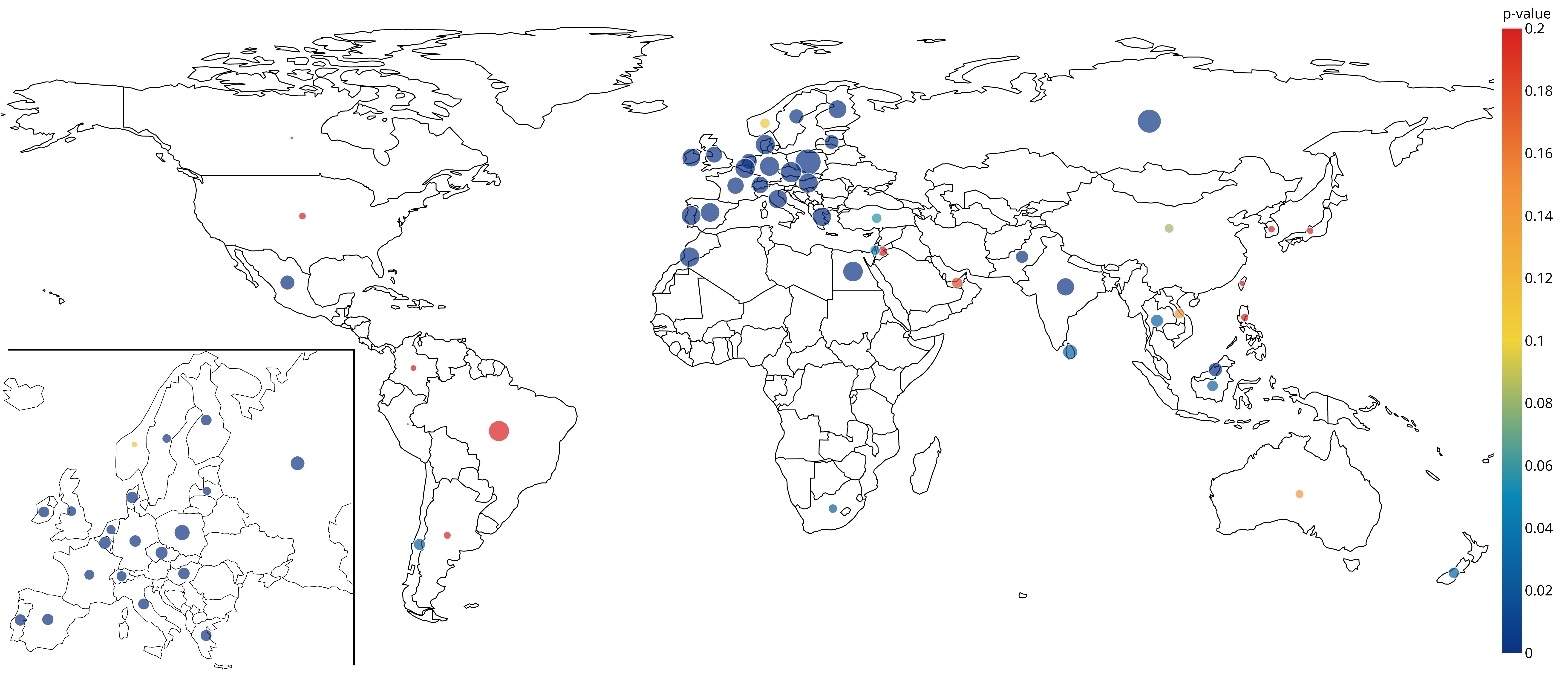
Figure 2: The significance and size of the impact the conflict attention index on future volatility at the onset-of-invasion – worldwide

Notes: The size of a circle is determined by the coefficient estimate of $C_{t}$, relative to the largest observed value. The color denotes the statistical significance in terms of the p-value of the $C_{t}$ coefficient estimate. With all p-values higher than 0.2 being statistically insignificant, these values were capped at 0.2 to facilitate graphical presentation.

Figure 3: The importance of conflict attention independence to economic connectedness with Russia and geographical distance

Notes: On the y-axis, we use the absolute value of the t-statistic for estimated parameter $C_{t}$ during the onset-of-invasion sample. We excluded Latvia from the chart for better graphical representation because its DOO value places it far from the other observations. However, this decision does not bias the presented results in any way.

Based on the results in Table 3, the day-ahead volatility is most significantly affected by conflict attention at the onset of the invasion period in ten European countries. In addition, we find that all European countries in our dataset except for Norway are highly impacted. In fact, the effect is concentrated in Europe and near the military conflict, which is also visible in Figure 2. We assume that these countries might be influenced due to strong economic ties with Russia, the threat of wider European conflict with the possible involvement of NATO or the ongoing humanitarian crisis (with a few million refugees fleeing Ukraine). Of the countries facing a wave of refugees, our analysis covers Poland, Czechia, Hungary, and Germany, all of which are among the most impacted countries. The previously mentioned dependence of Europe on oil and gas imports from Russia may also be an important reason why this conflict has primarily affected European stock markets. This argument is particularly supported by the fact that we have not found a significant impact on Norway, which is independent of Russia due to the former’s substantial oil and gas reserves.

However, in the pre-invasion period, the conflict attention variable was not significant at the 5 % level for any of the countries considered. This statement is also valid for wartime data for the countries extracted in Table 4. These are primarily American and Asian countries. Regarding the variable representing the previous day’s volatility $V_{t}$, despite the significance of this parameter for many countries in the before invasion period, $V_{t}$ became insignificant for most of the indices during the onset-of-invasion.

There are also some significantly impacted countries outside of Europe, for instance, Mexico, whose results could be explained by the fact that Mexico did not condemn the Russian invasion (Reuters, 2022b). Various reasons could explain the impact of the conflict in other countries. We have, for example, countries that are dependent on wheat imports from Ukraine, or those, that like Russia, extract oil.

Based on these findings, we assume that the effect of the conflict attention variable increases the geographically closer the country is to Russia or the stronger its relations are with Russia. Firstly, we decided to graphically verify this relationship in Figure 3, which displays the relationship between the conflict attention t-value of each country and its economic openness with Russia and between the conflict attention t-value and its geographical distance from Moscow. Based on these charts, we conclude that the more open a country is to Russia, meaning a higher ratio of Russian imports and exports to the country’s GDP, the more significant that conflict attention is. Conversely, conflict attention is less significant for countries that are more geographically distant from the Russian capital.
Secondly, appropriate tests were carried out. More specifically, we estimate the panel regression defined by Equation 9 for both variables $DOO_{i}$ and $Dist_{i}$. We are interested in the significance of the parameter $\beta_{5}$ as well as in its sign. Presented in Table 5, the $\beta_{5}$ is significant in both panel regressions. The sign in case of the interaction term $C_{i,t}Dist_{i}$ is negative, and in case of $C_{i,t}DOO_{i}$ positive. This is in perfect alignment with Figure 3. Simply put, marginal effect of a change in $Dist_{i}$ on day-ahead volatility is $\beta_{5}C_{i,t}$, thus for an arbitrary $C_{i,t}$ (which is always positive) we are affected less by $C_{i,t}$ with the growing distance from Moscow. Analogically, the same interpretation holds for $DOO_{i}$, but with the opposite effect.

Table 5: Panel regression to provide further evidence on findings in Figure 3

	FE-DK-DOO	FE-DK-Dist
$const$	$-3.125^{a}$	$-3.280^{b}$
$V_{i,t}$	$\textbf{0.193}^{c}$	$\textbf{0.187}^{c}$
$V^{w}_{i,t}$	0.153	$0.089$
$C_{i,t}$	$\textbf{0.207}^{c}$	$\textbf{0.454}^{d}$
$G_{i,t}$	$0.712$	$0.747^{a}$
$C_{i,t}DOO_{i}$	$\textbf{3.731}^{d}$
$C_{i,t}Dist_{i}$		$\textbf{-0.033}^{d}$
$R^{2}(within)$	0.236	0.249
$R^{2}(between)$	0.552	0.402
$F-statistic$	133.601	143.972

Notes: Superscripts $a$, $b$, $c$ and $d$ denote statistical significance of estimated coefficients at the 10%, 5%, 1% and 0.1% level.

3.1 Robustness checks of achieved results

Achieved results and their significance may be influenced by several factors of choice we had to make in order to conduct our analysis. The most crucial ones are the time-period split date, log transformation of price variation variables, and the likeliness of the results being driven only by the first few days of the invasion. Thus, we resorted to checking our results under different settings. We tried three different split dates (2021-12-01, 2021-12-15, and 2022-01-15), under which the results point to the same conclusions – the same hold for the no-log transformation of volatility measures. For controlling for the first week of the invasion, we introduce a dummy variable into model defined in Equation 7.

$$V_{t+1}=\beta_{0}+\beta_{1}V_{t}+\beta_{2}V_{t}^{w}+\beta_{3}C_{t}+\beta_{4}D_{t}C_{t}+\beta_{5}G_{t}+\epsilon_{t+1}$$ (10)

where we assign $D_{t}$ with ones for the first week of invasion starting on 21st February and also for 21st and 24th February separately. The conflict variable remained significant.

Further, we estimate the Equation 11, where in contrast to Equation 10, the effects of $D_{t}$ and $C_{t}$ are separated.

$$V_{t+1}=\beta_{0}+\beta_{1}V_{t}+\beta_{2}V_{t}^{w}+\beta_{3}C_{t}+\beta_{4}D_{t}+\beta_{5}G_{t}+\epsilon_{t+1}$$ (11)

In this setup, we control for any external effect that may occur during the first week of the invasion, but is not contained by any of our independent variables. With the $\beta_{4}$ being mostly insignificant across the 51 countries. The only difference we observe is in case of Turkey and Israel, which $\beta_{3}$ became less significant, meaning there could be another factor we did not account for in these two countries. Results of other countries remains unchanged.

Furthermore, in our main results, we employ the attention variables of international investors measured by worldwide Google Trends. To verify whether this attention was in fact international, we estimate our models again with country-specific conflict attention $C_{t}$ retrieved with location specified only for the country of the given MSCI index. Panel data regression with local conflict attention confirms our findings, as the results are nearly identical to those with international attention. On the other hand, for individual countries we find slight differences, which could be extended in future research.

4 Conclusion

This paper explores how investors’ attention to the conflict between Russia and Ukraine influences the variability of asset prices in specific countries. We construct a Google search-based military conflict attention variable and general stock market attention to capture the effect of excessive attention devoted to the conflict. To draw sharp conclusions about volatility, we applied an HAR-RV model with a range-volatility estimator to MSCI data.

Our results demonstrate that while the impact of the conflict attention measure was insignificant in the pre-invasion period, at a time of escalating war threats, attention to conflict significantly affects volatility. Specifically, increasing conflict attention leads to higher volatility of the indices of the studied countries. The analysis of the indicators of the economic and geographical interconnectedness of individual countries to Russia shows that the effect of attention is more significant in countries with higher openness with Russia and those nearer to it.

Future scope of the research may contain the study of volatility spillover effect among markets, as our results showed that for 36 countries, conflict attention variable is significant, which can be caused by contagion, similar to studies Pericoli and Sbracia (2003); Diebold and Yilmaz (2009, 2012); Lyócsa et al. (2020a); Okorie and Lin (2021). Our findings may also be applied in the context of portfolio asset allocation, which utilizes methods of Google Trends as Kristoufek (2013); Maggi and Uberti (2021) or with adding the information regarding sentiment, the methods like Dumas et al. (2009); Song et al. (2017); Yu et al. (2022). Finally, our findings may prove to be useful in the domain of option pricing as a better volatility estimate leads to a more appropriate option price (Cretarola et al., 2020).

Appendix A Appendix

The list of general attention topics is as follows: ’asset allocation’, ’Bloomberg’, ’day trading’, ’dividend yield’, ’earnings call’, ’earnings per share’, ’exchange-traded fund’, ’financial crisis’, ’financial market’, ’futures contract’, ’Google Finance’, ’government bond’, ’hedge fund’, ’Implied volatility’, ’market capitalization’, ’market liquidity’, ’market sentiment’, ’MSCI’, ’mutual fund’, ’option contract’, ”pension fund’, ’price–earnings ratio’, ’quarterly finance report’, ’stock market index’, ’stock market’, ’technical analysis’, ’ticker symbol’, ’VIX’, ’volatility’, ’Yahoo! Finance’, and ’yield curve’.

Table 6: Further results with significant conflict attention variable $C_{t}$

	IRL	EGY	ESP	DEU	MAR	NLD	CHE	MEX	IND	MYS	FRA	LVA	PAK	SWE	RUS
Panel A: OLS parameters estimates – during war period
Constant	-5.577	-1.471	-5.929	-2.858	4.633	-1.449	-3.285	$\textbf{-9.526}^{c}$	$\textbf{-9.169}^{b}$	0.210	-2.308	$\textbf{-8.870}^{a}$	-3.000	-0.240	7.026
$V_{t}$	0.011	$\textbf{0.313}^{a}$	0.152	0.081	0.055	0.099	0.127	0.158	0.033	-0.010	$\textbf{0.265}^{a}$	-0.039	0.235	0.168	0.122
$V_{t}^{w}$	-0.098	-0.462	-0.191	-0.131	0.014	-0.397	-0.301	-0.182	-0.147	0.232	-0.057	0.731	$\textbf{-0.636}^{b}$	0.031	0.121
$C_{t}$	$\textbf{0.625}^{d}$	$\textbf{0.740}^{d}$	$\textbf{0.679}^{d}$	$\textbf{0.707}^{d}$	$\textbf{0.725}^{d}$	$\textbf{0.466}^{d}$	$\textbf{0.535}^{d}$	$\textbf{0.396}^{d}$	$\textbf{0.582}^{d}$	$\textbf{0.362}^{d}$	$\textbf{0.527}^{d}$	$\textbf{0.380}^{d}$	$\textbf{0.309}^{d}$	$\textbf{0.406}^{c}$	$\textbf{1.006}^{c}$
$G_{t}$	1.389	0.070	1.325	0.490	-1.882	0.509	0.621	$\textbf{2.344}^{c}$	$\textbf{2.116}^{b}$	-0.473	0.429	$\textbf{2.066}^{a}$	0.628	0.033	-1.670
Panel A1: Estimated models diagnostics
$R^{2}$	0.502	0.438	0.554	0.570	0.466	0.359	0.425	0.556	0.536	0.412	0.620	0.494	0.262	0.436	0.669
$adj.R^{2}$	0.452	0.364	0.510	0.528	0.413	0.297	0.368	0.513	0.488	0.350	0.583	0.444	0.190	0.379	0.636
residual $\rho(1)$	0.120	0.198	0.022	0.089	-0.001	0.079	0.072	-0.045	0.110	-0.110	0.086	0.038	0.004	0.046	0.076
Ljung-Box	0.691	0.514	0.133	0.907	0.861	0.917	0.331	0.017	0.060	0.775	0.877	0.902	0.256	0.985	0.469
White	0.287	0.780	0.967	0.061	0.668	0.104	0.102	0.947	0.399	0.338	0.454	0.001	0.500	0.459	0.690
Panel B: Parameters estimates of the same model using pre-invasion data sample
Constant	$\textbf{-3.524}^{b}$	-3.362	-2.815	-0.652	-0.040	-3.825	-1.159	$\textbf{-5.427}^{d}$	-2.202	-1.898	-3.393	$\textbf{11.049}^{a}$	$\textbf{-3.295}^{a}$	-1.160	$\textbf{-3.363}^{b}$
$V_{t}$	0.113	$\textbf{0.213}^{a}$	0.147	$\textbf{0.207}^{b}$	0.115	$\textbf{0.174}^{a}$	0.170	$\textbf{0.181}^{a}$	$\textbf{0.308}^{c}$	0.065	0.094	0.062	$\textbf{0.200}^{b}$	$\textbf{0.345}^{d}$	0.079
$V_{t}^{w}$	$\textbf{0.311}^{b}$	0.184	0.339	0.225	0.301	$\textbf{0.441}^{c}$	$\textbf{0.319}^{b}$	0.212	0.228	0.250	$\textbf{0.509}^{c}$	0.197	$\textbf{0.483}^{d}$	$\textbf{0.288}^{a}$	$\textbf{0.545}^{d}$
$C_{t}$	$\textbf{-0.496}^{a}$	-0.075	-0.107	0.141	-0.296	-0.251	0.151	-0.117	-0.063	-0.061	-0.154	$\textbf{0.697}^{a}$	$\textbf{-0.402}^{a}$	-0.060	0.183
$G_{t}$	$\textbf{0.875}^{a}$	0.898	0.662	-0.029	-0.310	0.939	0.127	$\textbf{1.385}^{d}$	0.463	0.205	0.739	$\textbf{-3.142}^{b}$	$\textbf{0.863}^{a}$	0.223	$\textbf{0.864}^{b}$
Panel B1: Estimated models diagnostics
$R^{2}$	0.104	0.105	0.123	0.104	0.072	0.206	0.154	0.170	0.200	0.032	0.177	0.048	0.309	0.281	0.306
$adj.R^{2}$	0.076	0.068	0.096	0.077	0.043	0.182	0.128	0.145	0.175	0.002	0.153	0.018	0.288	0.259	0.285
residual $\rho(1)$	0.007	0.008	0.008	0.010	0.003	-0.005	-0.016	0.043	0.030	-0.009	0.006	-0.008	-0.065	-0.061	0.006
Ljung-Box	0.132	0.998	0.610	0.908	0.038	0.622	0.792	0.880	0.113	0.733	0.597	0.909	0.238	0.470	0.013
White	0.320	0.420	0.000	0.275	0.924	0.031	0.005	0.429	0.786	0.008	0.000	1.000	0.356	0.005	0.009

Notes: In the header, we use ISO 3166 country codes. Regression parameter estimates in bold indicate significance at the 10% level; superscripts $a$, $b$, $c$ and $d$ denote statistical significance of estimated coefficients at the 10%, 5%, 1% and 0.1% level. Residuals $\rho(1)$ describe the first-order autocorrelation of the residuals. For the Ljung-Box and White tests, we report the corresponding p-values.

Table 7: Further results with less- or in-significant conflict attention variable $C_{t}$

	HKG	ZAF	CHL	NZL	IDN	LKA	THA	SGP	ISR	TUR	CHN	NOR	AUS	VNM	ARE	USA
Panel A: OLS parameters estimates – during war
Constant	-5.332	$\textbf{-4.269}^{a}$	$\textbf{-5.595}^{b}$	-3.369	-3.751	-3.274	$\textbf{-4.999}^{a}$	$\textbf{-8.351}^{b}$	$\textbf{-12.086}^{c}$	-3.442	-2.869	$\textbf{-6.179}^{b}$	$\textbf{-9.089}^{b}$	-3.183	0.202	$\textbf{-13.040}^{c}$
$V_{t}$	$\textbf{0.474}^{b}$	-0.180	-0.113	0.073	-0.070	0.045	-0.215	0.238	$\textbf{-0.350}^{b}$	0.044	$\textbf{0.562}^{c}$	0.095	0.278	0.011	0.128	$\textbf{0.294}^{b}$
$V_{t}^{w}$	$\textbf{-1.878}^{a}$	$\textbf{0.529}^{a}$	-0.493	0.284	-0.011	0.123	0.373	-0.150	-0.114	-0.414	$\textbf{-0.703}^{a}$	0.140	-0.082	0.461	0.061	-0.066
$C_{t}$	$\textbf{0.635}^{b}$	$\textbf{0.157}^{b}$	$\textbf{0.258}^{b}$	$\textbf{0.229}^{b}$	$\textbf{0.235}^{b}$	$\textbf{0.398}^{b}$	$\textbf{0.294}^{b}$	$\textbf{0.250}^{b}$	$\textbf{0.182}^{a}$	$\textbf{0.192}^{a}$	$\textbf{0.165}^{a}$	0.189	0.141	-0.197	0.226	0.099
$G_{t}$	0.769	0.970	$\textbf{1.677}^{b}$	0.747	0.783	0.984	0.939	$\textbf{1.961}^{b}$	$\textbf{3.227}^{d}$	1.172	0.663	$\textbf{1.474}^{a}$	$\textbf{2.129}^{b}$	0.954	-0.283	$\textbf{3.314}^{c}$
Panel A1: Estimated models diagnostics
$R^{2}$	0.368	0.283	0.246	0.337	0.200	0.301	0.326	0.331	0.340	0.159	0.307	0.282	0.308	0.269	0.115	0.353
$adj.R^{2}$	0.306	0.213	0.172	0.268	0.116	0.223	0.257	0.266	0.276	0.077	0.240	0.212	0.236	0.185	0.028	0.286
residual $\rho(1)$	0.081	0.023	-0.021	-0.064	0.037	-0.004	0.093	0.021	0.071	-0.027	-0.146	-0.025	-0.059	0.016	-0.033	-0.073
Ljung-Box	0.976	0.893	0.920	0.984	0.825	0.001	0.827	0.239	0.109	0.714	0.018	0.468	0.832	0.645	0.787	0.572
White	0.237	0.357	0.157	0.535	0.653	0.794	0.026	0.077	0.287	0.786	0.674	0.123	0.767	0.654	0.309	0.495
Panel B: Parameters estimates of the same model using pre-invasion data sample
Constant	-2.657	-1.966	-2.037	-2.477	$\textbf{-3.705}^{b}$	$\textbf{-3.348}^{a}$	-2.054	$\textbf{-4.134}^{a}$	$\textbf{-13.124}^{c}$	-1.489	-1.722	$\textbf{-4.839}^{b}$	-2.646	$\textbf{3.486}^{b}$	-0.483	-1.707
$V_{t}$	0.176	0.125	0.104	0.077	0.076	$\textbf{0.202}^{a}$	0.144	0.135	-0.001	$\textbf{0.237}^{a}$	$\textbf{0.238}^{b}$	0.113	$\textbf{0.315}^{d}$	$\textbf{0.183}^{a}$	0.170	$\textbf{0.425}^{d}$
$V_{t}^{w}$	0.191	0.181	0.140	$\textbf{0.338}^{a}$	0.225	$\textbf{0.335}^{b}$	$\textbf{0.359}^{b}$	0.134	$\textbf{0.576}^{b}$	$\textbf{0.599}^{d}$	0.263	$\textbf{0.288}^{a}$	-0.136	$\textbf{0.358}^{b}$	$\textbf{0.228}^{a}$	0.158
$C_{t}$	-0.169	-0.342	0.109	-0.084	-0.200	0.208	$\textbf{-0.506}^{c}$	0.428	0.164	0.188	0.061	0.198	-0.039	$\textbf{0.455}^{b}$	$\textbf{0.603}^{a}$	0.162
$G_{t}$	0.533	0.441	0.614	0.524	$\textbf{0.877}^{b}$	$\textbf{0.837}^{a}$	0.409	0.888	$\textbf{3.282}^{b}$	0.370	0.415	$\textbf{1.124}^{b}$	0.413	$\textbf{-0.886}^{b}$	-0.055	0.279
Panel B1: Estimated models diagnostics
$R^{2}$	0.057	0.061	0.026	0.070	0.072	0.228	0.127	0.100	0.249	0.550	0.131	0.161	0.096	0.267	0.170	0.276
$adj.R^{2}$	0.029	0.031	-0.003	0.041	0.044	0.204	0.099	0.073	0.227	0.535	0.105	0.135	0.068	0.245	0.136	0.253
residual $\rho(1)$	0.014	-0.007	-0.003	-0.011	-0.020	-0.025	-0.020	0.023	0.046	-0.023	-0.004	0.018	0.024	0.004	0.022	-0.080
Ljung-Box	0.679	0.425	0.994	0.132	0.225	0.561	0.461	0.167	0.801	0.152	0.800	0.646	0.592	0.884	0.423	0.481
White	0.782	0.000	0.759	0.030	0.840	0.458	0.121	0.086	0.000	0.103	0.702	0.000	0.299	0.832	0.832	0.703

Notes: In the header, we use ISO 3166 country codes. Regression parameter estimates in bold indicate significance at the 10% level; superscripts $a$, $b$, $c$ and $d$ denote statistical significance of estimated coefficients at the 10%, 5%, 1% and 0.1% level. Residuals $\rho(1)$ describe the first-order autocorrelation of the residuals. For the Ljung-Box and White tests, we report the corresponding p-values.

Table 8: Descriptive statistics of daily price variation estimates $V_{t}$

Country	Mean	S.D.	Median	Min.	Max.	$\rho(1)$	$\rho(5)$
MEX	1.386	1.573	0.952	0.080	14.892	0.297	0.096
TWN	0.742	0.694	0.545	0.047	4.935	0.122	0.006
VNM	2.374	2.949	1.550	0.140	21.005	0.336	0.206
LVA	2.094	13.852	0.436	0.000	178.848	0.224	0.280
POL	1.903	4.026	0.821	0.098	40.368	0.596	0.244
NLD	1.747	2.485	0.962	0.052	19.410	0.530	0.288
ESP	1.442	2.431	0.755	0.062	24.491	0.277	0.205
JOR	1.193	2.269	0.478	0.033	16.052	0.051	-0.098
CHL	3.335	8.850	1.864	0.000	104.034	0.032	-0.005
ARE	0.865	2.105	0.389	0.047	19.848	0.116	-0.021
GRC	1.217	1.681	0.752	0.111	12.780	0.283	0.198
ISR	1.182	2.083	0.678	0.001	19.732	0.146	0.219
JPN	0.777	0.677	0.580	0.077	4.000	0.299	0.192
SGP	0.686	0.704	0.487	0.004	5.379	0.330	0.101
EGY	1.979	2.477	1.272	0.105	15.377	0.255	0.285
MYS	0.296	0.267	0.214	0.034	1.841	0.245	0.084
FIN	1.439	2.700	0.664	0.049	24.208	0.399	0.410
BRA	3.420	2.793	2.647	0.000	19.316	0.380	-0.052
RUS	24.636	119.963	1.350	0.149	1305.617	0.294	0.244
KOR	0.742	0.687	0.510	0.083	5.219	0.350	0.065
PER	2.664	3.056	1.851	0.274	23.346	0.233	-0.076
PRT	1.514	2.043	0.965	0.117	19.941	0.403	0.240
CAN	0.531	0.833	0.266	0.030	7.395	0.501	0.031
DEU	0.896	1.602	0.364	0.027	14.705	0.429	0.446
CHE	0.754	1.225	0.364	0.042	9.587	0.410	0.150
IRL	1.948	3.835	0.954	0.100	42.090	0.475	0.213
MAR	0.275	0.522	0.116	0.009	4.389	0.361	0.138
IND	0.905	1.295	0.524	0.061	12.761	0.330	0.197
HKG	0.700	0.811	0.477	0.001	7.215	0.178	-0.012
AUS	0.459	0.570	0.311	0.057	6.195	0.393	-0.011
CZE	0.982	1.864	0.425	0.036	19.126	0.435	0.323
BEL	1.062	2.139	0.458	0.076	18.469	0.349	0.237
IDN	0.866	0.692	0.686	0.079	4.826	0.150	0.064
PHL	0.948	1.061	0.610	0.048	8.059	0.292	-0.081
ITA	1.180	2.553	0.510	0.047	28.591	0.504	0.496
CHN	1.244	1.117	0.923	0.039	8.078	0.445	0.131
TUR	3.252	8.524	1.250	0.145	77.889	0.659	0.089
NZL	0.793	0.787	0.561	0.076	6.595	0.331	0.171
USA	0.840	1.375	0.406	0.006	12.228	0.460	0.117
ARG	4.824	5.258	3.072	0.305	35.770	0.491	0.228
DNK	1.788	2.995	0.955	0.103	26.473	0.164	0.092
FRA	0.976	1.723	0.440	0.036	16.661	0.507	0.452
COL	1.994	2.211	1.284	0.001	17.012	0.247	-0.015
SWE	1.331	2.323	0.589	0.066	22.986	0.456	0.254
GBR	0.544	0.694	0.304	0.028	5.649	0.392	0.292
HUN	3.392	9.141	1.072	0.110	70.508	0.731	0.511
PAK	1.722	1.717	1.180	0.178	12.174	0.442	0.186
THA	0.502	0.491	0.388	0.102	4.421	0.454	0.031
ZAF	0.868	0.660	0.647	0.067	4.874	0.197	-0.001
LKA	3.035	5.642	1.064	0.084	42.756	0.567	0.302
NOR	0.860	1.014	0.497	0.045	9.059	0.214	0.123

Notes: Countries are denoted by ISO 3166 country codes. S.D. stands for standard deviation, and $\rho(n)$ is an autocorrelation coefficient of the $n$th order.

References

- Aalborg et al. (2019) Aalborg, H.A., Molnár, P., de Vries, J.E., 2019. What can explain the price, volatility and trading volume of bitcoin? Finance Research Letters 29, 255–265. URL: https://linkinghub.elsevier.com/retrieve/pii/S1544612318302058, doi:10.1016/j.frl.2018.08.010.
- Andersen et al. (2003) Andersen, T.G., Bollerslev, T., Diebold, F.X., Labys, P., 2003. Modeling and forecasting realized volatility. Econometrica 71, 579–625.
- Andrei and Hasler (2015) Andrei, D., Hasler, M., 2015. Investor attention and stock market volatility. Review of Financial Studies 28, 33–72. URL: https://academic.oup.com/rfs/article-lookup/doi/10.1093/rfs/hhu059, doi:10.1093/rfs/hhu059.
- Aouadi et al. (2013) Aouadi, A., Arouri, M., Teulon, F., 2013. Investor attention and stock market activity: Evidence from france. Economic Modelling 35, 674–681. URL: https://linkinghub.elsevier.com/retrieve/pii/S0264999313003507, doi:10.1016/j.econmod.2013.08.034.
- Audrino et al. (2020) Audrino, F., Sigrist, F., Ballinari, D., 2020. The impact of sentiment and attention measures on stock market volatility. International Journal of Forecasting 36, 334–357. URL: https://linkinghub.elsevier.com/retrieve/pii/S0169207019301645, doi:10.1016/j.ijforecast.2019.05.010.
- Baig et al. (2019) Baig, A., Blau, B.M., Sabah, N., 2019. Price clustering and sentiment in bitcoin. Finance Research Letters 29, 111–116.
- Barber and Odean (2008) Barber, B.M., Odean, T., 2008. All that glitters: The effect of attention and news on the buying behavior of individual and institutional investors. Review of Financial Studies 21, 785–818. URL: https://academic.oup.com/rfs/article-lookup/doi/10.1093/rfs/hhm079, doi:10.1093/rfs/hhm079.
- Ben-Rephael et al. (2017) Ben-Rephael, A., Da, Z., Israelsen, R.D., 2017. It Depends on Where You Search: Institutional Investor Attention and Underreaction to News. The Review of Financial Studies 30, 3009–3047. URL: https://academic.oup.com/rfs/article/30/9/3009/3830159, doi:10.1093/rfs/hhx031.
- Bijl et al. (2016) Bijl, L., Kringhaug, G., Molnár, P., Sandvik, E., 2016. Google searches and stock returns. International Review of Financial Analysis 45, 150–156. URL: https://linkinghub.elsevier.com/retrieve/pii/S105752191630045X, doi:10.1016/j.irfa.2016.03.015.
- Bordino et al. (2012) Bordino, I., Battiston, S., Caldarelli, G., Cristelli, M., Ukkonen, A., Weber, I., 2012. Web search queries can predict stock market volumes. PLoS ONE 7. URL: https://dx.plos.org/10.1371/journal.pone.0040014, doi:10.1371/journal.pone.0040014.
- Bowen (2022) Bowen, A.S., 2022. Russian Military Buildup Along the Ukrainian Border. Technical Report IN11806. Congressional Research Service. URL: https://crsreports.congress.gov/product/pdf/IN/IN11806.
- Burggraf et al. (2020) Burggraf, T., Huynh, T.L.D., Rudolf, M., Wang, M., 2020. Do fears drive bitcoin? Review of Behavioral Finance doi:10.1108/RBF-11-2019-0161.
- Cheah and Fry (2015) Cheah, E.T., Fry, J., 2015. Speculative bubbles in bitcoin markets? an empirical investigation into the fundamental value of bitcoin. Economics Letters 130, 32–36. URL: https://linkinghub.elsevier.com/retrieve/pii/S0165176515000890, doi:10.1016/j.econlet.2015.02.029.
- Chen et al. (2020) Chen, C., Liu, L., Zhao, N., 2020. Fear sentiment, uncertainty, and bitcoin price dynamics: The case of covid-19. Emerging Markets Finance and Trade 56, 2298–2309. URL: https://doi.org/10.1080/1540496X.2020.1787150, doi:10.1080/1540496X.2020.1787150.
- Corsi (2009) Corsi, F., 2009. A simple approximate long-memory model of realized volatility. Journal of Financial Econometrics 7, 174–196.
- Cretarola et al. (2020) Cretarola, A., Figà-Talamanca, G., Patacca, M., 2020. Market attention and bitcoin price modeling: Theory, estimation and option pricing. Decisions in Economics and Finance 43, 187–228.
- Da et al. (2011) Da, Z., Engelberg, J., Gao, P., 2011. In search of attention. The Journal of Finance 66, 1461–1499. URL: http://doi.wiley.com/10.1111/j.1540-6261.2011.01679.x, doi:10.1111/j.1540-6261.2011.01679.x.
- Diebold and Yilmaz (2009) Diebold, F.X., Yilmaz, K., 2009. Measuring financial asset return and volatility spillovers, with application to global equity markets. The Economic Journal 119, 158–171.
- Diebold and Yilmaz (2012) Diebold, F.X., Yilmaz, K., 2012. Better to give than to receive: Predictive directional measurement of volatility spillovers. International Journal of forecasting 28, 57–66.
- Dimpfl and Jank (2016) Dimpfl, T., Jank, S., 2016. Can internet search queries help to predict stock market volatility? European Financial Management 22, 171–192. URL: http://doi.wiley.com/10.1111/eufm.12058, doi:10.1111/eufm.12058.
- Driscoll and Kraay (1998) Driscoll, J.C., Kraay, A.C., 1998. Consistent covariance matrix estimation with spatially dependent panel data. Review of economics and statistics 80, 549–560.
- Dugas et al. (2013) Dugas, A.F., Jalalpour, M., Gel, Y., Levin, S., Torcaso, F., Igusa, T., Rothman, R.E., 2013. Influenza forecasting with google flu trends. PLoS ONE 8, e56176. URL: https://dx.plos.org/10.1371/journal.pone.0056176, doi:10.1371/journal.pone.0056176.
- Dumas et al. (2009) Dumas, B., Kurshev, A., Uppal, R., 2009. Equilibrium portfolio strategies in the presence of sentiment risk and excess volatility. The Journal of Finance 64, 579–629.
- Eom et al. (2019) Eom, C., Kaizoji, T., Kang, S.H., Pichl, L., 2019. Bitcoin and investor sentiment: Statistical characteristics and predictability. Physica A: Statistical Mechanics and its Applications 514, 511–521. URL: https://doi.org/10.1016/j.physa.2018.09.063, doi:10.1016/j.physa.2018.09.063.
- Fricke et al. (2014) Fricke, E., Fung, S., Goktan, M.S., 2014. Google search, information uncertainty, and post-earnings announcement drift. Journal of Accounting and Finance 14, 11.
- Garcia et al. (2014) Garcia, D., Tessone, C.J., Mavrodiev, P., Perony, N., 2014. The digital traces of bubbles: feedback cycles between socio-economic signals in the bitcoin economy. Journal of The Royal Society Interface 11, 20140623. URL: https://royalsocietypublishing.org/doi/10.1098/rsif.2014.0623, doi:10.1098/rsif.2014.0623, arXiv:1408.1494.
- Garman and Klass (1980) Garman, M.B., Klass, M.J., 1980. On the estimation of security price volatilities from historical data. Journal of business , 67–78.
- Ginsberg et al. (2009) Ginsberg, J., Mohebbi, M.H., Patel, R.S., Brammer, L., Smolinski, M.S., Brilliant, L., 2009. Detecting influenza epidemics using search engine query data. Nature 457, 1012–1014. URL: http://www.nature.com/articles/nature07634, doi:10.1038/nature07634.
- Goddard et al. (2015) Goddard, J., Kita, A., Wang, Q., 2015. Investor attention and fx market volatility. Journal of International Financial Markets, Institutions and Money 38, 79–96. URL: https://linkinghub.elsevier.com/retrieve/pii/S1042443115000542, doi:10.1016/j.intfin.2015.05.001.
- Hamid and Heiden (2015) Hamid, A., Heiden, M., 2015. Forecasting volatility with empirical similarity and google trends. Journal of Economic Behavior & Organization 117, 62–81. URL: https://linkinghub.elsevier.com/retrieve/pii/S0167268115001687, doi:10.1016/j.jebo.2015.06.005.
- Han et al. (2018) Han, L., Xu, Y., Yin, L., 2018. Does investor attention matter? the attention-return relationships in fx markets. Economic Modelling 68, 644–660. URL: https://linkinghub.elsevier.com/retrieve/pii/S0264999317310027, doi:10.1016/j.econmod.2017.06.015.
- Harris and Sonne (2021) Harris, S., Sonne, P., 2021. Russia planning massive military offensive against ukraine involving 175,000 troops, u.s. intelligence warns. URL: https://www.proquest.com/blogs-podcasts-websites/russia-planning-massive-military-offensive/docview/2605794001/se-2?accountid=16531. name - North Atlantic Treaty Organization–NATO; Copyright - Copyright WP Company LLC d/b/a The Washington Post Dec 4, 2021; Last updated - 2021-12-04.
- Hirshleifer et al. (2011) Hirshleifer, D., Lim, S.S., Teoh, S.H., 2011. Limited Investor Attention and Stock Market Misreactions to Accounting Information. Review of Asset Pricing Studies 1, 35–73. URL: https://academic.oup.com/raps/article-lookup/doi/10.1093/rapstu/rar002, doi:10.1093/rapstu/rar002.
- Hirshleifer and Sheng (2021) Hirshleifer, D., Sheng, J., 2021. Macro news and micro news: Complements or substitutes? Journal of Financial Economics d. URL: https://linkinghub.elsevier.com/retrieve/pii/S0304405X21004001, doi:10.1016/j.jfineco.2021.09.012.
- IEA (2022) IEA, 2022. International energy agency: How europe can cut natural gas imports from russia significantly within a year. Contify Energy News URL: https://www.proquest.com/magazines/international-energy-agency-how-europe-can-cut/docview/2637699407/se-2?accountid=16531. name - International Energy Agency; European Union; Copyright - Copyright 2017 Contify.com; Last updated - 2022-03-10.
- Joseph et al. (2011) Joseph, K., Babajide Wintoki, M., Zhang, Z., 2011. Forecasting abnormal stock returns and trading volume using investor sentiment: Evidence from online search. International Journal of Forecasting 27, 1116–1127. URL: http://dx.doi.org/10.1016/j.ijforecast.2010.11.001, doi:10.1016/j.ijforecast.2010.11.001.
- Kapounek et al. (2021) Kapounek, S., Kučerová, Z., Kočenda, E., 2021. Selective attention in exchange rate forecasting. Journal of Behavioral Finance 0, 1–19. URL: https://www.tandfonline.com/doi/full/10.1080/15427560.2020.1865355, doi:10.1080/15427560.2020.1865355.
- Kita and Wang (2012) Kita, A., Wang, Q., 2012. Investor attention and fx market volatility. SSRN Electronic Journal 44. doi:10.2139/ssrn.2022100.
- Kristoufek (2013) Kristoufek, L., 2013. Can Google Trends search queries contribute to risk diversification? Scientific Reports 3, 2713. URL: http://www.nature.com/articles/srep02713, doi:10.1038/srep02713, arXiv:1310.1444.
- Kristoufek (2015) Kristoufek, L., 2015. What are the main drivers of the bitcoin price? evidence from wavelet coherence analysis. PLoS ONE 10, 1–15. doi:10.1371/journal.pone.0123923, arXiv:1406.0268.
- Lister (2021) Lister, T., 2021. Satellite photos raise concerns of russian military build-up near ukraine. URL: https://www.proquest.com/wire-feeds/satellite-photos-raise-concerns-russian-military/docview/2592901220/se-2?accountid=16531. name - Department of Defense; North Atlantic Treaty Organization–NATO; Copyright - Copyright 2021 Cable News Network. Turner Broadcasting System, Inc. All Rights Reserved; Last updated - 2021-11-04.
- Liu et al. (2021) Liu, H., Peng, L., Tang, Y., 2021. Retail attention, institutional attention. Journal of Financial and Quantitative Analysis, forthcoming .
- Lyócsa et al. (2021) Lyócsa, Š., Baumöhl, E., Vỳrost, T., 2021. Yolo trading: Riding with the herd during the gamestop episode. Finance Research Letters , 102359.
- Lyócsa et al. (2020a) Lyócsa, Š., Baumöhl, E., Výrost, T., Molnár, P., 2020a. Fear of the coronavirus and the stock markets. Finance Research Letters 36, 101735. URL: https://doi.org/10.1016/j.frl.2020.101735, doi:10.1016/j.frl.2020.101735.
- Lyócsa et al. (2020b) Lyócsa, Š., Molnár, P., Plíhal, T., Širaňová, M., 2020b. Impact of macroeconomic news, regulation and hacking exchange markets on the volatility of bitcoin. Journal of Economic Dynamics and Control 119, 103980. URL: https://linkinghub.elsevier.com/retrieve/pii/S0165188920301482, doi:10.1016/j.jedc.2020.103980.
- Lyócsa and Plíhal (2022) Lyócsa, Š., Plíhal, T., 2022. Russia’s Ruble during the onset of the Russian invasion of Ukraine in early 2022: The role of implied volatility and attention. arXiv preprint arXiv:2205.09179 .
- Maggi and Uberti (2021) Maggi, M., Uberti, P., 2021. Google search volumes for portfolio management: performances and asset concentration. Annals of Operations Research 299, 163–175.
- Mao et al. (2011) Mao, H., Counts, S., Bollen, J., 2011. Predicting financial markets: Comparing survey, news, twitter and search engine data , 1–10URL: http://arxiv.org/abs/1112.1051, arXiv:1112.1051.
- Massicotte and Eddelbuettel (2021) Massicotte, P., Eddelbuettel, D., 2021. gtrendsR: Perform and Display Google Trends Queries. URL: https://CRAN.R-project.org/package=gtrendsR. r package version 1.4.8.
- Newey and West (1987) Newey, W.K., West, K.D., 1987. A simple, positive semi-definite, heteroskedasticity and autocorrelation consistent covariance matrix. Econometrica 55, 703–708. URL: http://www.jstor.org/stable/1913610.
- Okorie and Lin (2021) Okorie, D.I., Lin, B., 2021. Stock markets and the covid-19 fractal contagion effects. Finance Research Letters 38, 101640.
- Olearchyk et al. (2022) Olearchyk, R., Foy, H., Politi, J., 2022. Us accuses russia of planning ‘false-flag operation’ in eastern ukraine. FT.com URL: https://www.proquest.com/trade-journals/us-accuses-russia-planning-false-flag-operation/docview/2628042984/se-2?accountid=16531. copyright - Copyright The Financial Times Limited Jan 14, 2022; Last updated - 2022-02-13; SubjectsTermNotLitGenreText - Russia; United States–US; Ukraine.
- Parkinson (1980) Parkinson, M., 1980. The extreme value method for estimating the variance of the rate of return. Journal of business , 61–65.
- Patton and Sheppard (2009) Patton, A.J., Sheppard, K., 2009. Optimal combinations of realised volatility estimators. International Journal of Forecasting 25, 218–238.
- Pericoli and Sbracia (2003) Pericoli, M., Sbracia, M., 2003. A primer on financial contagion. Journal of economic surveys 17, 571–608.
- Pesaran (2007) Pesaran, M.H., 2007. A simple panel unit root test in the presence of cross-section dependence. Journal of applied econometrics 22, 265–312.
- Plíhal (2021) Plíhal, T., 2021. Scheduled macroeconomic news announcements and Forex volatility forecasting. Journal of Forecasting , 1–19doi:10.1002/for.2773.
- Preis et al. (2013) Preis, T., Moat, H.S., Stanley, H.E., 2013. Quantifying trading behavior in financial markets using google trends. Scientific Reports 3, 1684. URL: http://www.nature.com/articles/srep01684, doi:10.1038/srep01684.
- Preis et al. (2010) Preis, T., Reith, D., Stanley, H.E., 2010. Complex dynamics of our economic life on different scales: insights from search engine query data. Philosophical Transactions of the Royal Society A: Mathematical, Physical and Engineering Sciences 368, 5707–5719. URL: https://royalsocietypublishing.org/doi/10.1098/rsta.2010.0284, doi:10.1098/rsta.2010.0284.
- Reuters (2022a) Reuters, 2022a. Extracts from putin’s speech on ukraine. URL: https://www.reuters.com/world/europe/extracts-putins-speech-ukraine-2022-02-21/.
- Reuters (2022b) Reuters, 2022b. Mexico declines to impose economic sanctions on russia. URL: https://www.reuters.com/world/mexicos-president-says-will-not-take-any-economic-sanctions-against-russia-2022-03-01/.
- Rodriguez (2000) Rodriguez, C.A., 2000. On the degree of openness of an open economy. Universidad del CEMA .
- Rogers and Satchell (1991) Rogers, L.C.G., Satchell, S.E., 1991. Estimating variance from high, low and closing prices. The Annals of Applied Probability , 504–512.
- Salama et al. (2022) Salama, V., Michaels, D., Norman, L., 2022. Russia says it sees little scope for optimism in u.s. proposals on ukraine – wsj. URL: https://www.proquest.com/wire-feeds/russia-says-sees-little-scope-optimism-u-s/docview/2623216763/se-2?accountid=16531. name - North Atlantic Treaty Organization–NATO; Copyright - Copyright Dow Jones & Company Inc Jan 27, 2022; Last updated - 2022-01-28.
- Saxena and Chakraborty (2020) Saxena, K., Chakraborty, M., 2020. Should we pay attention to investor attention in forex futures market? Applied Economics 52, 6562–6572. URL: https://www.tandfonline.com/doi/full/10.1080/00036846.2020.1804050, doi:10.1080/00036846.2020.1804050.
- Shalal et al. (2021) Shalal, A., Holland, S., Osborn, A., 2021. Biden warns putin of sanctions, aid for ukraine military if russia invades. URL: https://www.reuters.com/markets/currencies/biden-putin-set-crucial-call-over-ukraine-2021-12-07/.
- Simon and Davies (2022) Simon, S.C., Davies, L., 2022. ‘we need bread’: fears in middle east as ukraine war hits wheat imports. URL: https://www.proquest.com/blogs-podcasts-websites/we-need-bread-fears-middle-east-as-ukraine-war/docview/2637040803/se-2?accountid=16531. copyright - Copyright Guardian News & Media Limited Mar 7, 2022; Last updated - 2022-03-08.
- Smith (2012) Smith, G.P., 2012. Google internet search activity and volatility prediction in the market for foreign currency. Finance Research Letters 9, 103–110. URL: http://dx.doi.org/10.1016/j.frl.2012.03.003, doi:10.1016/j.frl.2012.03.003.
- Song et al. (2017) Song, Q., Liu, A., Yang, S.Y., 2017. Stock portfolio selection using learning-to-rank algorithms with news sentiment. Neurocomputing 264, 20–28.
- Urquhart (2018) Urquhart, A., 2018. What causes the attention of bitcoin? Economics Letters 166, 40–44. URL: https://linkinghub.elsevier.com/retrieve/pii/S016517651830065X, doi:10.1016/j.econlet.2018.02.017.
- Vlastakis and Markellos (2012) Vlastakis, N., Markellos, R.N., 2012. Information demand and stock market volatility. Journal of Banking & Finance 36, 1808–1821. URL: https://linkinghub.elsevier.com/retrieve/pii/S0378426612000507, doi:10.1016/j.jbankfin.2012.02.007.
- Wu et al. (2019) Wu, Y., Han, L., Yin, L., 2019. Our currency, your attention: Contagion spillovers of investor attention on currency returns. Economic Modelling 80, 49–61. URL: https://linkinghub.elsevier.com/retrieve/pii/S0264999317317236, doi:10.1016/j.econmod.2018.05.012.
- Yu et al. (2022) Yu, J.R., Chiou, W.P., Hung, C.H., Dong, W.K., Chang, Y.H., 2022. Dynamic rebalancing portfolio models with analyses of investor sentiment. International Review of Economics & Finance 77, 1–13.